Satellite-Observed Chlorophyll-a Concentration Variability in the East Sea (Japan Sea): Seasonal Cycle, Long-Term Trend, and Response to Climate Index

Introduction

Climate change and oceanic warming have increasingly influenced in marine ecosystems by modifying the physical environment in which phytoplankton grow (e.g., Baker et al., 2004; Doney et al., 2012; Bindoff et al., 2019). Sea surface temperature (SST) and sea level are representative oceanic imprints of global warming and have been consistently changing over recent decades (Church et al., 2013; Bulgin et al., 2020). SST has been increasing at the rate of 0.012°C yr^–1 which has contributed to changes in marine ecosystems (National Oceanic and Atmospheric Administration [NOAA], 2016). Alterations in the vertical stratification of the oceanic surface layer and surface current advection have modified nutrient supply and photon distribution required for phytoplankton photosynthesis in the sunlit ocean layers (Laws and Bannister, 1980; Dutkiewicz et al., 2013, 2019; Behrenfeld et al., 2016).

The responses of the marine ecosystem in the global ocean have been extensively studied over the past two decades by using long-term satellite data and in situ measurements including nutrient levels, SST, surface currents, vertical temperature and salinity profiles, and sea surface winds driving seawater (Gregg et al., 2003; Rivas et al., 2006; Patti et al., 2010; Kubryakov et al., 2016; Gohin et al., 2019; Yu et al., 2019; Garcia-Eidell et al., 2021). These measurements have been made using various cruise programs in the global ocean and regional seas (Kim et al., 2001; Werdell and Bailey, 2005; Peloquin et al., 2013; Zhang et al., 2018; Sloyan et al., 2019). However, in situ measurements have limited coverage of marginal seas and there is high multispatial-scale variability in local ecosystems (Zhou et al., 2018). Satellite ocean color measurements have furnished valuable, spatially extensive, repeatable, and simultaneous regional-scale data. These measurements combined with satellite chlorophyll-a (Chl-a) concentration data have been used to monitor spatiotemporal variability in marine phytoplankton. Chl-a concentration data have been widely applied to analyze low-level ecosystems in the global ocean and local seas (Son et al., 2006; Alvain et al., 2008; Schaeffer et al., 2008; McClain, 2009; Siegel et al., 2013; Li et al., 2018; Hammond et al., 2020).

The East Sea (Japan Sea; hereafter, EJS) is a miniature model of the global ocean. It is characterized by diverse oceanic phenomena, a zonally distributed subpolar front, and well-developed warm and cold current systems, such as the East Korea Warm Current, the Tsushima Warm Current, the Primorye Cold Current, and the North Korea Cold Current (Figure 1; Ichiye, 1984; Kim et al., 2001; Park et al., 2013). As the EJS is located between the largest continent (Eurasia) and the largest ocean (the Pacific) on Earth, it has been exposed to climate change and global warming over a very long period of time and has undergone rapid change in recent decades (Gamo, 2011). The linkage between large-scale and regional-scale change should have a significant impact on the physical environment and the marine ecosystem of the EJS. Large-scale variations in atmospheric pressure differences between the Pacific High and its associated wind field strengthen cold water upwelling and Chl-a bloom off the southeastern coast of Korea (Hyun et al., 2009; Yoo and Park, 2009; Kim et al., 2014). These extreme events may be evidence of linkages between large-scale atmospheric forcing and local biological responses manifested by changes in the physical environment of the local seas (Park and Kim, 2010; Park and Lee, 2014). Satellite ocean color data are expected to clarify phytoplankton responses to climate change in the EJS.

FIGURE 1

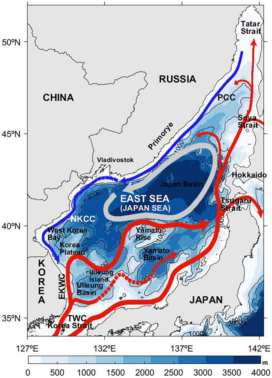
Figure 1. Surface current system over the bathymetry (m) of the East Sea (Japan Sea). Red (blue) solid lines represent warm (cold) currents. Gray solid line indicates that surface currents are connected to deep currents. Dashed lines represent seasonal differences and highly variable spatial distributions. EKWC, East Korea Warm Current; NKCC, North Korean Cold Current; PCC, Primorye Cold Current; TWC, Tsushima Warm Current. The current map is from Park et al. (2013).

The Coastal Zone Color Scanner (CZCS) of Nimbus-7 and Sea-viewing Wide Field-of-view Sensor (SeaWiFS) are satellite ocean color sensors used to examine the biosphere. The Moderate Resolution Imaging Spectroradiometer (MODIS) has generated ocean color data since 2002 and is extensively utilized. In the seas around Korea, complex oceanic and atmospheric conditions have affected seasonal and interannual variations in satellite-observed Chl-a (Yamaguchi et al., 2012, 2013; Liu et al., 2014; Wang et al., 2015). In the study region, long-term trends and spatiotemporal variability in Chl-a concentrations were investigated by Empirical Orthogonal Function (EOF) analysis and linear regression (Park et al., 2020a). Variability in the Chl-a concentration of the EJS has been explained by the mechanisms and interactions of sea-surface wind field, mixed layer depth, stratification, and nutrient distribution (Yamada et al., 2004; Yamada and Ishizaka, 2006; Kim et al., 2007; Jo et al., 2014; Lee et al., 2014; Park et al., 2014). Changes in the physical environment play key roles in the spatiotemporal variability of Chl-a concentrations in local seas (May et al., 2003; Kouketsu et al., 2015; Park et al., 2020a). Wind forcing influences the Chl-a dynamics of meso-scale eddies by modifying wind speeds and divergence/convergence and vorticity fields (Martin and Richards, 2001; McGillicuddy et al., 2007; Gaube et al., 2013; Frenger et al., 2013; Park et al., 2016, 2020b). However, none of the previous studies has addressed the spatial distribution of the quantitative responses of satellite-observed variations in Chl-a concentration to climate index variability in the entire EJS region.

Therefore, it is meaningful to analyze the responses of Chl-a concentration to elucidate the ocean color changes associated with climate change. In addition, the seasonal cycles and long-term trends of Chl-a variations must be estimated by excluding seasonal to interannual variations from Chl-a concentration variability in the EJS. The present study examined how the response patterns of low-level ecosystems can be extracted from highly changeable Chl-a concentration variability by considering large-scale connectivity processes in equatorial and Arctic regions. The objectives of this study were to investigate annual, semi-annual, and intraseasonal Chl-a concentrations cycles, clarify their contributions to total variance, understand how large interannual variations modify the estimation of long-term trends in Chl-a concentration in the EJS, and investigate long-term trends in sea surface wind (SSW) vectors and SST. Also this study depicts the spatial distribution of the responses of the Chl-a concentration to the Arctic Oscillation (AO) and the El Niño-Southern Oscillation (ENSO), and determine their relationships with SST anomalies in response to tropic-to-extratropic and Arctic-to-subarctic interactions.

Data and Methods

Satellite Data and Climate Index

The MODIS of the Aqua satellite has generated ocean color variables and stable global ocean data since 2002. Remote sensing reflectance (Rrs) and MODIS Level-2 path Chl-a concentration data were furnished by the National Aeronautics and Space Administration/Ocean Biology Processing Group (NASA/OBPG) and utilized in the present study,¹ with good performances in terms of accuracy (Vogelzang et al., 2011; Verhoef et al., 2012; Verspeek et al., 2012). To understand the variability of Chl-a concentration in the EJS, the research area (34–52°N, 127–143°E) was selected by encompassing the southern part of the Korea and Tatar Strait in the northern EJS. Chl-a concentration data for 2003–2020 were used. Monthly SSW field data were obtained by taking the average of the wind vectors at each grid and using the wind vector cell data of MetOp-A/B ASCAT (Advanced Scatterometer) from the EUMETSAT Ocean and Sea Ice Satellite Application Facility (OSISAF). An understanding changes in the physical environment has been achieved by using daily SST data from the Multi-scale Ultra-high Resolution SST (MURSST) of the Jet Propulsion Laboratory (JPL)/National Aeronautics and Space Administration (NASA).

A time series of the Multivariate ENSO Index (MEI) index (MEI.v2 values) from 2003 to 2020 was used as an ENSO index (Wolter and Timlin, 2011).² The AO index data were obtained from Climate Prediction Center of NOAA (CPC/NOAA) for the study period (e.g., Thompson and Wallace, 2000). The AO index comprised another representative climate index and their impacts on Chl-a concentration variability was investigated. To understand temporal variability of the climate indices, we obtained continuous wavelet transforms (CWT) of the AO and MEI indices using generalized Morse wavelets (GMWs) (Olhede and Walden, 2002).

Optimally Interpolated Monthly Chlorophyll-a Concentration Data

The typical cloud patterns of the EJS excluded data for its eastern part along the Japanese coast especially in winter. Near the cloud edges, highly anomalous Chl-a concentrations occasionally appeared because of difficulties in atmospheric correction. These problems frequently led to abnormally high Chl-a concentrations. The few speckles detected were removed to eliminate abnormal values (Park et al., 2020a). The Chl-a concentration data were composited by the weighted average method to yield L3 monthly data (Campbell et al., 1995) as follows:

$\overline{X}=\frac{1}{W}\sum _{i=1}^N\frac{1}{\sqrt{n_i}}\sum _{j=1}^{n_i}{X}_{ij}(1)$

$W=\sum _{i=1}^N\sqrt{n_i}(2)$

where $\overline{X}$ is the weighted average of the Chl-a concentration (X_ij), W is the sum of weights, i is the time t_i (i = 1,…, N), and j refers to the jth observation at time t_i (j = 1,…, n_i).

Considering the cloud coverage during summer and winter in the study area, 3-D optimal interpolation (OI) was implemented to obtain monthly composite maps using a spatial interval of 4.5 km and a time interval of 15 d. The fundamental OI equation [Chl-a ($x_k^a$)] was derived from another equation using the background field ($x_k^b$), the background error covariance matrix (B), the observation operator (H_k) connecting the model grid to the observation locations, the observation error covariance matrix (R_k), and the observations (y_k) (Donlon et al., 2012) as follows:

$x_k^a=x_k^b+{\mathit{BH}}_k^T{\left[H_k{\mathit{BH}}_k^T+R_k\right]}^{-1}\left(y_k-H_k{x}_k^b\right)(3)$

where R_k and the background field ($x_k^b$) were disregarded. OI was performed by applying a cross-covariance matrix of distances between grid points and satellite data and an autocovariance matrix of satellite data to an observation Chl-a concentration data matrix at each grid. The resultant monthly composite data were nearly the same as the original MODIS data except that the pixels with speckles were excluded.

Temporal Trend and Response to Climate Index

Spectral analysis of Fourier transform makes it possible to understand spectral power distribution by decomposing temporal variations into sinusoidal functions with various temporal frequencies. In contrast, harmonic analysis can extract the amplitudes and phases of a given time period. For example, the observation data y can be represented by n/2 sinusoidal functions oscillating around the mean value, as in the following formulation:

$y_t=\overline{y}+\sum _{i=1}^{n/2}\left[C_{i}cos\left(\frac{2\mathrm{\pi }it}{N}-{\mathrm{\theta }}_i\right)\right]=\overline{y}+\sum _{i=1}^{n/2}\left[F_{i}cos\left(\frac{2\mathrm{\pi }it}{n}\right)+G_{i}sin\left(\frac{2\mathrm{\pi }it}{n}\right)\right](4)$

where C_i is the amplitude ($=\sqrt{G_i^2+F_i^2}$), θ_i is the phase angle (= arctan(G_i/F_i)), and t is time. The combination of annual cycles from one to four cycles per year practically represents seasonal variation. These harmonics constitute major components of Chl-a concentration variations.

Considering these harmonics, temporal variations in MODIS Chl-a concentration per pixel were the results of various forcings and multifrequency oscillations such as intrinsic intraseasonal-to-seasonal variations, long-term trends, and interannual variations in climate indices. AO and MEI might be the main indices affecting the physical environment and marine ecosystem of the EJS. To extract the responses of Chl-a concentration to the climate index, a formula including multi-frequency variations was devised by considering the harmonics in the equation (4). A time series of Chl-a (Chla_t) per pixel consisted of annual harmonic constituents with coefficients (a_1,j, a_2,j) at four frequencies from 1 to 4 cycles yr^–1 (S_t), a linear trend (ω) (mg m^–3 yr^–1), components resonant to the AO and MEI indices, and a constant (μ) (Weatherhead et al., 1998; Bonjean and Lagerloef, 2002):

${\mathit{Chla}}_t=\mathrm{\mu }+\sum _{j=1}^4\left[a_{1,j}sin\left(\frac{2\mathrm{\pi }jt}{N}\right)+a_{2,j}cos\left(\frac{2\mathrm{\pi }jt}{N}\right)\right]+\frac{1}{N}\mathrm{\omega }t+\mathrm{\alpha }{E}_t+\mathrm{\beta }{A}_t(5)$

where ω is the increasing or decreasing rate of Chl-a concentration change (mg m^–3 yr^–1), N is the month number (12), and α and β are coefficients associated with the El Niño/Southern Oscillation (ENSO) (E_t) and the AO (A_t) indices, respectively. This method has long been applied and widely used on satellite SST data to understand ocean warming. As a result of a significance testing (Fisher, 1918), the p-values associated with the equation (5) approach were mostly statistically significant within the 95-percent confidence level as shown in Figure 2. The p-values were very small for the entire EJS, and in particular, the values reached 10^–25 and 10^–20 in the central part of the EJS (Figure 2A). Almost all grids showed small p-values less than 0.05. The pixels smaller than 0.05 accounted for 99.39% of the total area, and larger places accounted for only 0.60%, as indicated by a few gray dots in Figure 2A. Figure 2B shows a histogram of the p-values, showing statistical significance almost everywhere.

FIGURE 2

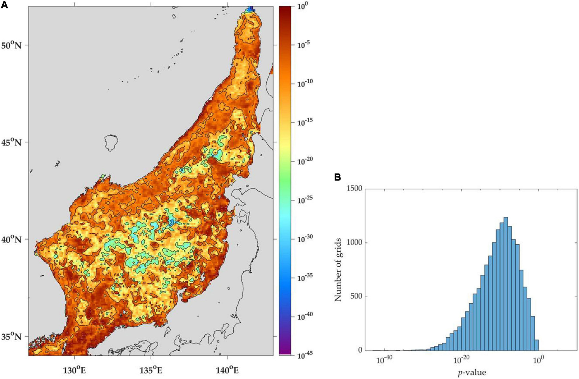
Figure 2. Spatial distribution of (A) statistical significance (p-values), based on multi-variate regression, of chlorophyll-a concentration data and (B) histogram of the p-values. Only a few statistically insignificant pixels (p-value < 0.05) are marked as gray dots in (A).

Results and Discussion

Mean and Temporal Variability of Chlorophyll-a Concentration

The bathymetry of the EJS is very deep (< 4,000 m) compared with that of the marginal seas of the Northwest Pacific. Hence, the seawater of the EJS is considered optically clear. Its optical properties are determined primarily by phytoplankton and colored dissolved organic matter (CDOM) (Mobley et al., 2004). Variability of the phytoplankton of the EJS may be evaluated from satellite-based Chl-a observations. The temporal mean of optimally interpolated monthly Chl-a data for 2003–2020 revealed low Chl-a (0.3–0.4 mg m^–3) in offshore regions such as the eastern part of the Japan Basin and the Tsushima Warm Current region (Figure 3A). Unlike the central part of the EJS, the relatively shallow continental shelf regions showed high Chl-a (2.0–4.0 mg m^–3) along the coastal regions of the Korean Peninsula, the Russian Primorye Coast, the Tatar Strait, and the Japanese Coast.

FIGURE 3

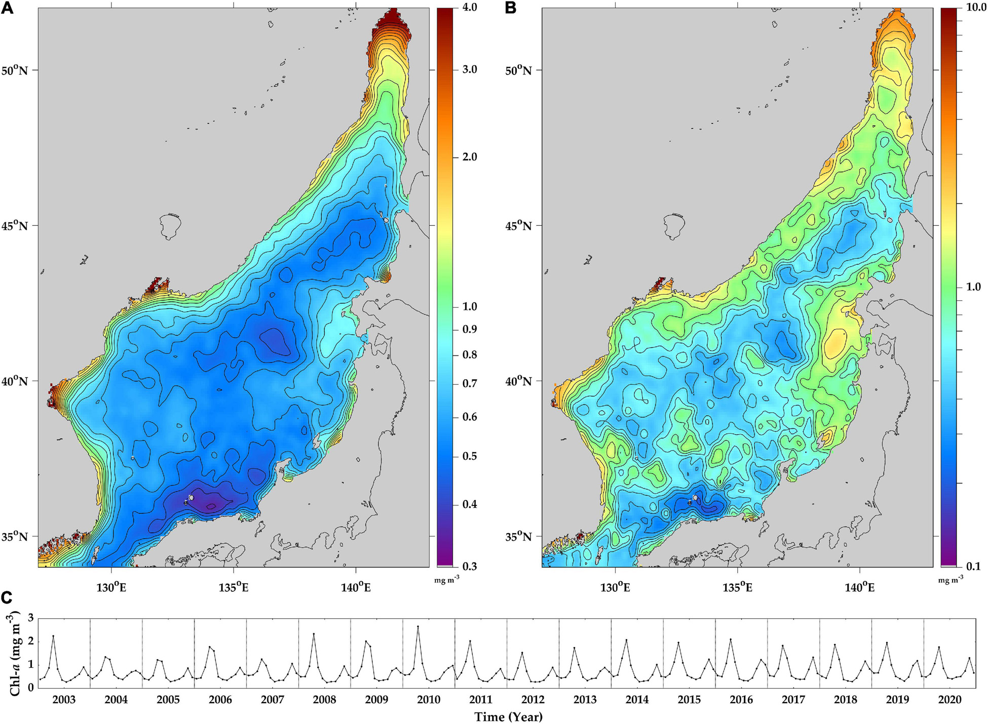
Figure 3. Spatial distributions of (A) temporal means, (B) temporal standard deviations, and (C) time series of spatial means of MODIS chlorophyll-a concentration in the East Sea (Sea of Japan) between 2003 and 2020.

Previous studies on temporal variations in the SST of the EJS demonstrated that the oceanic features of the EJS included a wide range of frequencies corresponding to intraseasonal, seasonal, and annual variations over decades (Park and Chung, 1999). In addition, sea surface height data from satellite altimetry indicated higher interannual than seasonal variations (Choi et al., 1999). The spatial distributions of the temporal Chl-a standard deviations demonstrated high variability (0.1–10 mg m^–3) far exceeding the mean Chl-a (Figure 3B). The continental shelf regions and certain parts of the offshore regions presented with high variability (5–10 mg m^–3). The magnitude of the temporal variability was ∼2–3 times greater than the mean values. The time-series of spatial mean Chl-a concentrations over the entire region showed both seasonal cycles and interannual variations (Figure 3C). The Chl-a variations with strong temporal variability are expected to dominate on longer time scales beyond the seasonal cycles.

Seasonal Variation and Annual Harmonics of Chlorophyll-a Concentration

The seasonal distribution of the Chl-a concentrations shows that phytoplankton density significantly increased in spring (April) relative to the other seasons (Figure 4). In spring, the Chl-a concentration reached 10 mg m^–3 mainly along the eastern coasts of the Korean Peninsula and Russia and the Tsushima Warm Current region. In summer (July), the Chl-a concentration declined to < 0.3 mg m^–3 throughout the entire EJS. However, when upwelling occurred in the southeastern and eastern coast of the Korean Peninsula in summer, the Chl-a spatially predominated (> 1.0 mg m^–3). Prevailing southerly or southeasterly winds drove Ekman transport to the offshore by increasing nutrient supply to the surface layers and caused the phytoplankton to flourish. In autumn (October), Chl-a increased again but to a much lesser extent than it did in springtime (Figure 4).

FIGURE 4

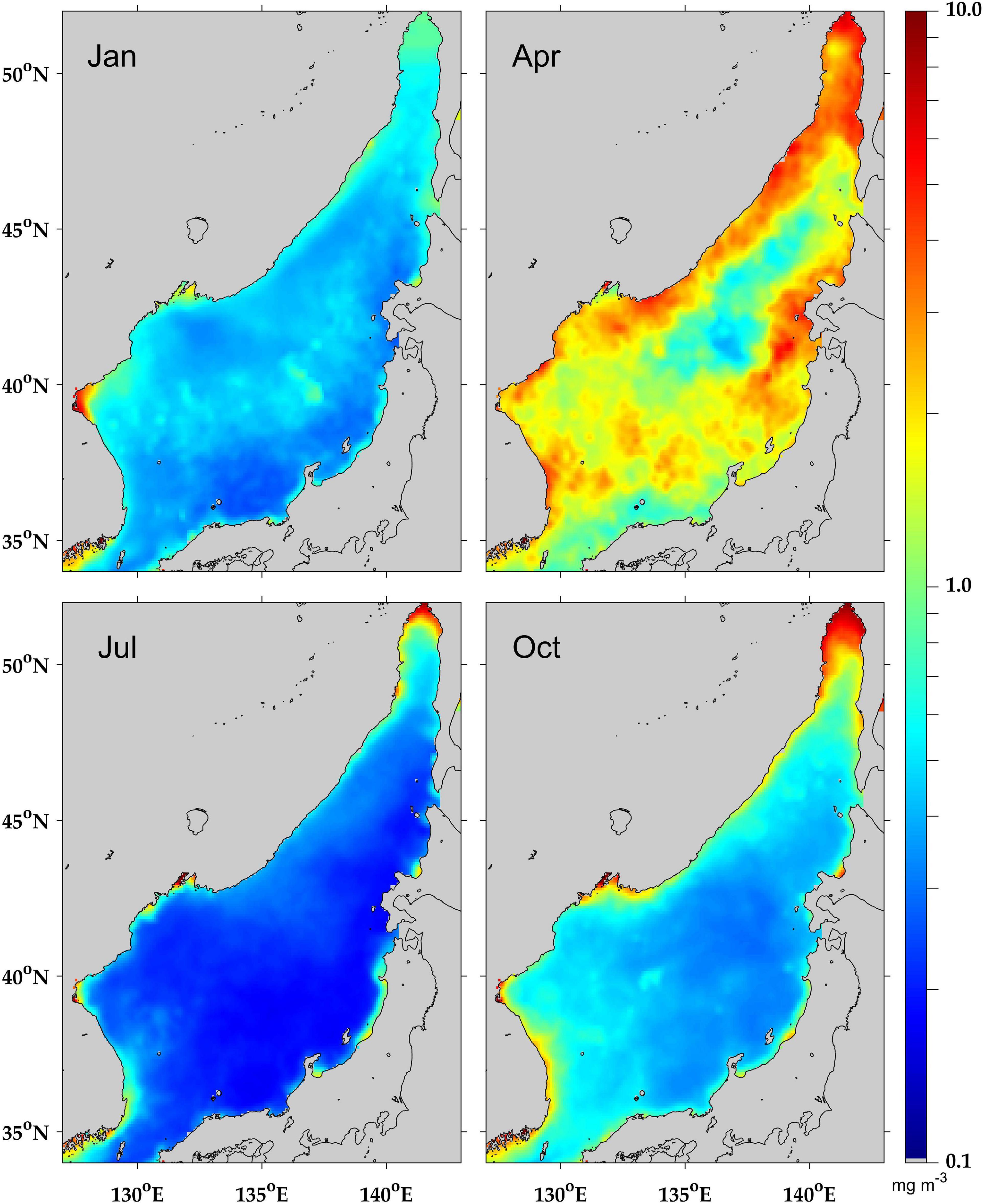
Figure 4. Seasonal distribution (mg m^–3) of phytoplankton chlorophyll-a concentrations calculated using satellite MODIS data for winter (January), spring (April), summer (July), and autumn (October) for the period of 2003–2020.

The Chl-a of the EJS demonstrated distinct seasonality and substantial phytoplankton bloom in spring. The temporal variability in Chl-a (Figure 3B) was much higher than the temporal mean Chl-a (Figure 3A) at each grid. Hence, there might have been greater interannual variations than seasonal changes in Chl-a. This seasonality may be calculated by applying harmonic analyses of the frequencies corresponding to 1–4 cycles yr^–1 quantified in the second term of Equation (5). Figure 5 shows the spatial distributions of the annual and semi-annual cycles of Chl-a variations. The amplitude of the annual cycle (1 cycle yr^–1) was in the range of 0.03–10 mg m^–3 with high frequency of 0.1–1.0 mg m^–3. It was relatively small of less than 0.3 mg m^–3 over the Japan Basin north of the subpolar front, extending zonally in the central part of the EJS, along the southern coastal region of the Korean Peninsula near the Korea Strait, and the southern region of the Tsushima Warm Current (Figure 5A). The harmonic amplitudes of the semi-annual cycle were high and greater than 1 mg m^–3 along the continental region off the Russian, the Korean Peninsula, and western region of the Tsugaru Strait and the southeastern part of the EJS west of Japan.

FIGURE 5

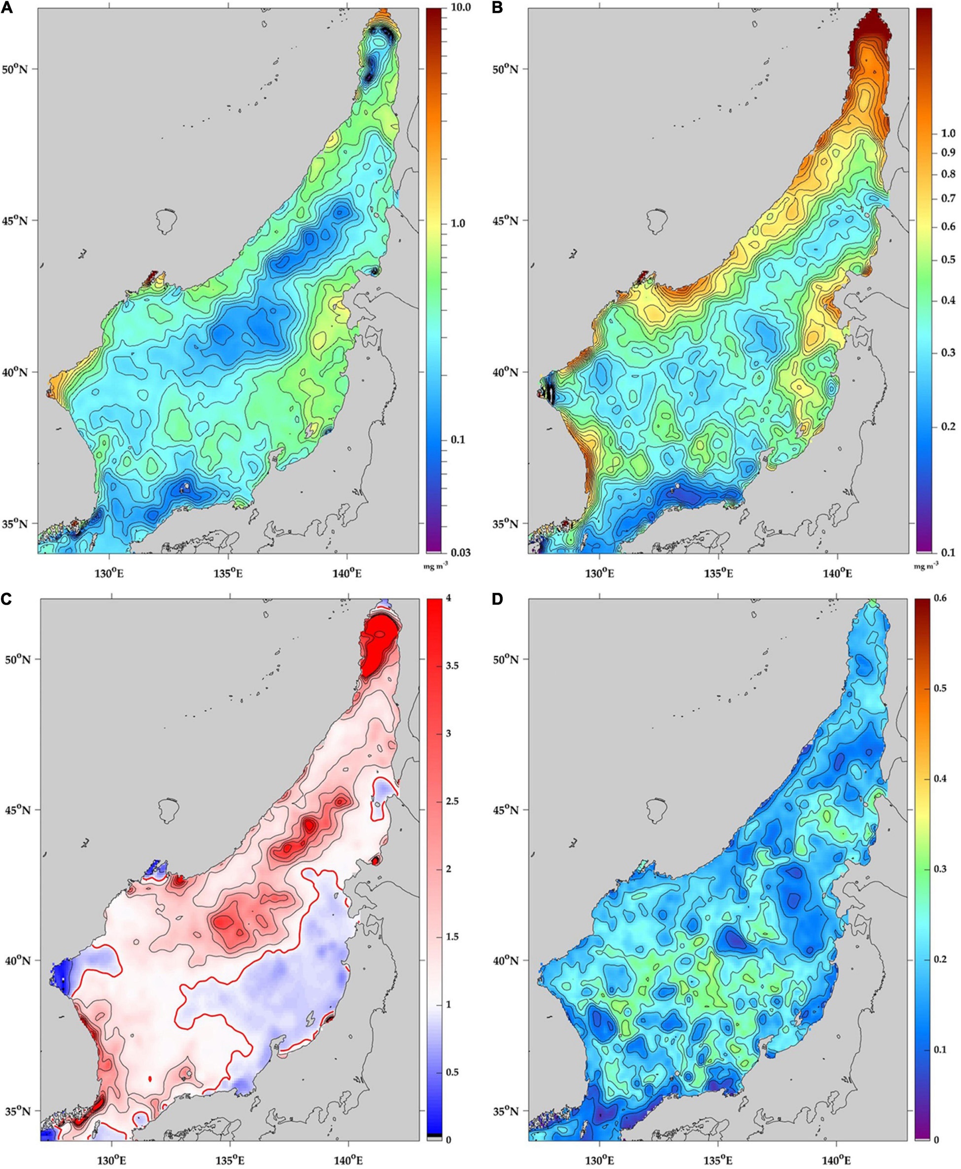
Figure 5. Spatial distribution of the amplitudes of the (A) annual cycle, (B) semi-annual cycle, (C) ratios of semi-annual to annual cycles, where the red contour corresponds to a ratio of 1.0, and (D) the ratios of the amplitudes (1–4 cycles per year) of seasonal variations to the total temporal variance of chlorophyll-a concentrations in the East Sea (Sea of Japan) for the period of 2003–2020.

The spatial distribution of the semi-annual Chl-a cycle resembled that of the annual cycle and resulted in spatially dominant features (0.0–2.0 mg m^–3) along the Russian and Korean continental shelf regions and the western region of Japan. However, the amplitude of the semi-annual cycle exceeded that of the annual cycle because of dominant spring and autumn phytoplankton blooms (Figure 5B). The ratio of the semi-annual to the annual amplitude at each pixel reached a maximum of > 3 (Figure 5C). On the eastern coast of Korea, high fractions of the semi-annual cycle appeared at similar ratios. The boundary region of the East Korea Warm Current (EKWC) had remarkable coastal fronts on the continental side. Another dominant region was found north of the central subpolar front (SPF), in the zonal direction along a latitude of approximately 40°N (Park et al., 2004), over the Japan Basin. Most of the northwestern part of the EJS showed fractions > 1, implying that the semi-annual Chl-a cycle had much higher amplitudes than the annual Chl-a cycle in those regions. By contrast, the eastern region of the EJS had ratios < 1. Hence, the semi-annual Chl-a cycle had equal or lower amplitudes compared with the annual Chl-a cycle (red contour; ratio = 1). Determination of the extent to which these seasonal cycles account for the total variance can clarify the contribution of non-seasonal Chl-a cycles to the annual fluctuations in the total Chl-a variability. Figure 5D shows the distribution of the ratios of the annual cycles (1–4 cycles per year) amplitude to the total variance of Chl-a variability. High ratios were detected in the central part and the TWC regions south of the SPF. Relatively small fractions of less than 0.2 (20%) appeared near the southern part of the EJS and along the coastlines near the land. This means that interannual variability is greater than that of seasonal variability in many parts of the EJS, which has not yet been well elucidated.

Chlorophyll-a Concentration Trends

The temporal trends in Chl-a concentrations have been investigated for the EJS region using MODIS data from 2003 to 2015 (Park et al., 2020a). However, that study adopted a linear trend in the Chl-a anomaly data simply by removing climatological data. In particular, large deviations from the climatology data at the beginning or end of time series data are likely to lead to an overestimation or underestimation of the actual long-term change. As in the previous literature describing the long-term estimation of SST warming (e.g., Weatherhead et al., 1998; Bonjean and Lagerloef, 2002), the trend in Chl-a should be calculated by considering yearly variations. We devised Equation (5) to calculate the temporal trend in Chl-a variation by excluding seasonal and annual Chl-a variations caused by variability in climate indices such as AO and ENSO. The oceanic features of the EJS appeared to markedly enhance annual variations that could affect the magnitudes of the long-term trends. To estimate how interannual changes contribute to the trend value, the trend was calculated from 2003 to 2013 and by increasing it year by year until 2020, and the differences from the existing method are quantitatively presented in Figure 6. For the 2003–2013 period (Figure 6A), the differences amounted to ± 0.015 mg m^–3 year^–1. As the period increased, the differences between the two trends decreased significantly. However, the differences still remained until 2020 as shown in the trend difference for the period of 2003–2020 (Figure 6H). These yearly variations signify that the interannual Chl-a variability should be eliminated for to understand the proper temporal trend.

FIGURE 6

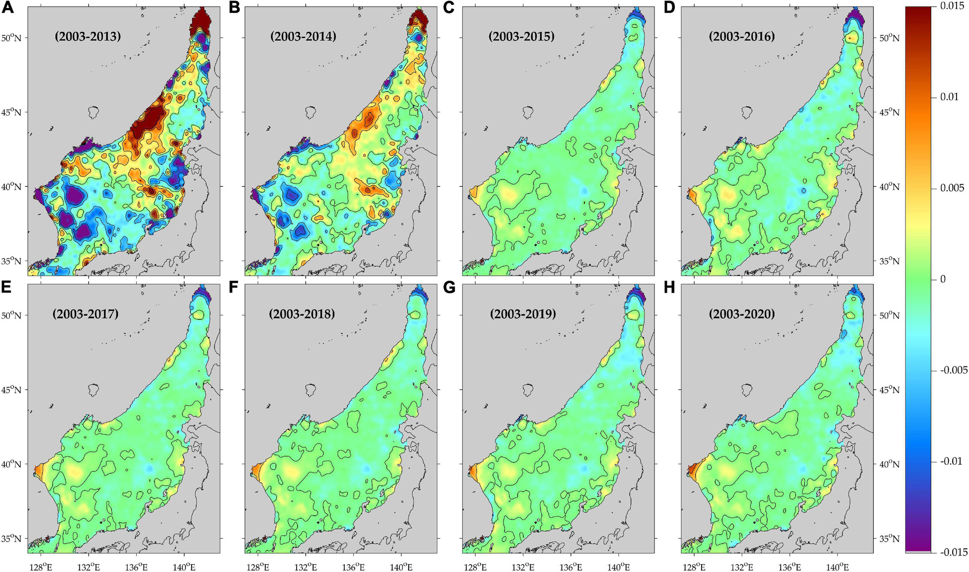
Figure 6. Spatial distribution of the differences in MODIS chlorophyll-a concentration trends (mg m⁻³ yr⁻¹) between ordinary trends and trends after removing seasonal to annual variations and (former minus latter) in the East Sea (Sea of Japan) for the periods of (A) 2003–2013, (B) 2003–2014, (C) 2003–2015, (D) 2003–2016, (E) 2003–2017, (F) 2003–2018, (G) 2003–2019, and (H) 2003–2020.

The temporal trend in Figure 7A shows the trends after excluding monthly Chl-a climatology for the given period (Park et al., 2020a). Most trends were statistically significant (p-value < 0.05) within the 95% confidence level The differences in the trends, ordinary trends minus multi-variational fitted trends, were significant when comprising 25% of the former trend. Specific areas with relatively high positive differences in Chl-a variations were detected in the eastern EJS and negative differences were detected in the western part of the EJS. Negative values in Figure 7B confirmed that previously reported long-term trends were considerably underestimated owing to non-seasonal variations based on longer time scales. This finding revealed the effects of interannual variations (expressed as climate indices) on the temporal trends. The longer-term temporal trends in Chl-a concentrations in Figure 7C revealed that most of the EJS changed to a more productive status, as inferred from the positive trends over most regions of the EJS. Especially, the near-continental regions along the Russian Primorye, the Tatar Strait, and the northern Korean Peninsula exhibited increasing temporal Chl-a trends (> 0.04 mg m^–3 year^–1). Negative trends, down to approximately -0.02 mg m^–3 year^–1, were detected in the southern part as the EKWC and the TWC regions (Figure 7C).

FIGURE 7

Figure 7. Spatial distribution of (A) MODIS chlorophyll-a concentration trends (mg m^–3 yr⁻¹) for the period 2003–2015 (Park et al., 2020a) and (B) differences in the trends, comprising oridinary trend minus multi-variational fitted trend in the East Sea (Sea of Japan) for the same period (2003–2015), and (C) trends in chlorophyll-a concentrations for the period 2003–2020.

The spatial distribution of the trends until 2015 showed remarkable negative trends on the east coast of the Korean Peninsula. However, when Chl-a data from 2003 to 2020 were used, it changed to positive trends that were evident in the entire area of the EJS (Figure 7C). This means that Chl-a variations in the EJS have changed rapidly in recent years. Therefore, the time change in the histograms of trends was analyzed by examining the number of grids representing positive and negative trends throughout the EJS from 2003 to the terminated years until 2020 (Figure 8A). It can be seen that over time until 2020, the maximum value of the histogram gradually moves to a positive trend, as shown by the red line (Figure 8A). This trend can also be seen in Figure 8B, with the number of grids with negative trends decreasing over time, whereas the number of grids with positive trends increased rapidly until 2016 and then became constant to 2020 (Figure 8B). As a result of calculating the spatial average in trends by period, this increased significantly from 2013 to 2016, and since then, it has shown an almost constant pattern (Figure 8C). As shown in Figure 7C, these positive changes were found in the northern area of the East Sea and on the east coast of the central part of the Korean Peninsula. Therefore, it is necessary to analyze what changes have occurred in the physical environment over the past 18 years in the EJS. To this end, changes in SST and SSW that can have a profound effect on chlorophyll fluctuations over the past decades have been investigated.

FIGURE 8

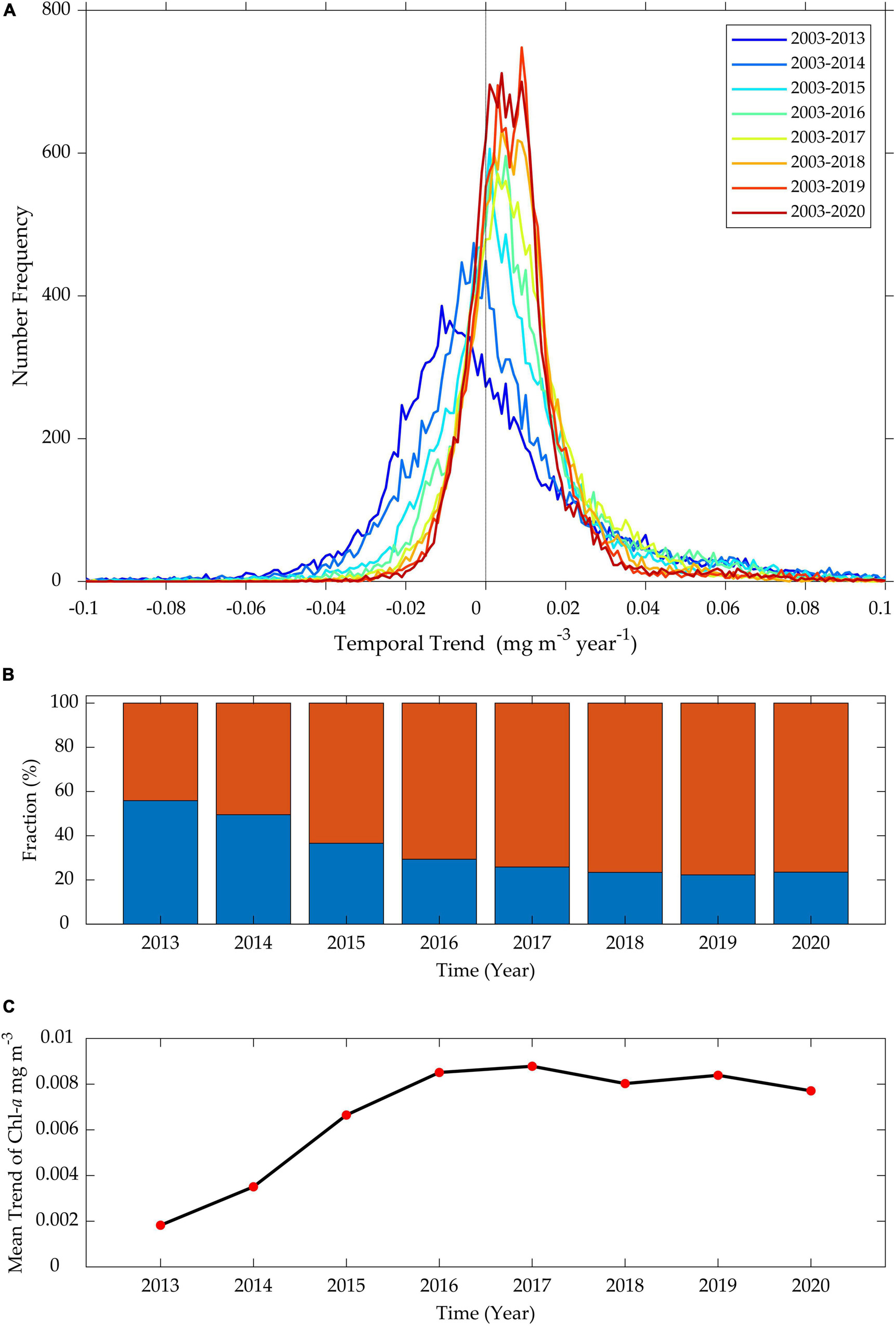
Figure 8. (A) Distribution of frequencies of temporal chlorophyll-a concentration (Chl-a) trends (mg m^–3 yr^–1) for the periods from 2003–2013 to 2003–2020, (B) yearly variations in fractions (%) of positive and negative trends (red and blue colors represent positive and negative trends, respectively), and (C) mean trends as a function of the end period.

Trends in Physical Environment: Sea Surface Temperature and Wind Field

Along With global ocean warming, the SST of the EJS also tended to increase Over the past few decades. According to a recent research result, specifically that the warming of the EJS Is continuously increasing, It Was found that the air temperature and SST in mid-latitude seas such as the EJS, in contrast, intermittently decreased further owing to the warming of the Arctic Ocean in winter (He et al., 2017; Lee and Park, 2019). as shown in Figure 9A, the SSTs of the EJS showed an increasing rate of up to 0.09°C in most areas of the southern EJS. Similar to the results of Lee and Park (2019), the SST showed negative trends of approximately -0.4 to -0.2°C in the vicinity of 40°N, 132°E, the offshore regions of Primorye, and the northeastern region of the EJS Over the past 18 years. It Can Be seen that the SSTs of the East Sea tended to gradually increase overall in the southern part but decreased in the northern part. Positive (negative) warming trends occupied 66.80% (33.20%) of the total spatial grids of the EJS. Considering this SST warming in the southern EJS, the surface layer Is more likely to provide a further vertically stratified environment than that in the past. However, the fact that the SST tended to decrease slightly in the northern part of the EJS means that nutrients, needed for phytoplankton growth, might Have Been supplied From the lower layer to the surface layer Over recent decades.

FIGURE 9

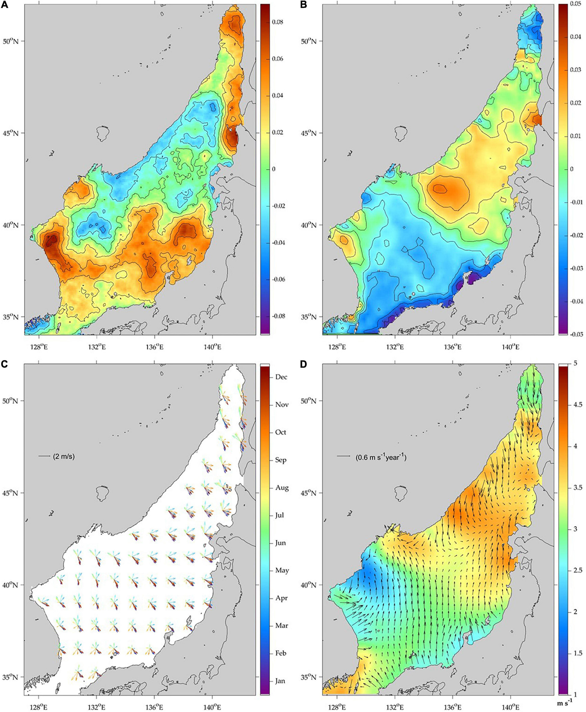
Figure 9. Spatial distributions of the temporal trends in (A) sea surface temperatures (°C year^–1) and (B) sea surface wind speeds (m s^–1 year^–1), (C) monthly variations in directional wind vectors (m s⁻¹) from January to December, and (D) directional trends in wind vectors (m s^–1 year^–1) in the East Sea (Japan Sea) from 2003 to 2020, where the background image represents the mean wind speeds.

This long-term trend in SST variations is mainly due to heat flux changes mediated by the SSW field. This long-term trend in SSTs is primarily due to changes in heat fluxes owing to wind forcing at the sea surface or the supply of heat from the surface currents. Figure 9B shows the results of the long-term trend in SSW, which played the most important role in SST changes. A positive increasing rate of up to 0.04 m s^–1 year^–1 appeared characteristically in the northeastern part of the East Sea. Another characteristic positive rate appeared as 0.03 in the regions off the central part of the Korean Peninsula. These positive wind trends covered 46% of the entire grids. However, a negative trend (∼0.04 m s^–1 year^–1) appeared as far as the Japanese coast, similar to the wind region blowing south from Vladivostok, Russia. In particular, off the coast of Japan, a negative trend of up to -0.05 m s^–1 year^–1 appeared as the wind speed weakened during the period from 2003 to 2020.

To understand the characteristics of temporal changes in wind forcing in more detail, the temporal trend in the wind direction vectors was also analyzed. As can be seen from the change in the monthly wind direction vectors in Figure 9C, the East Sea had strong seasonal variability with prevailing southerly or southeasterly winds in summer and northerly winds in winter. In Figure 9B, it is necessary to analyze the types of wind changes that have been derived from long-term trends in wind speed. It is also important to investigate which components of the wind direction vectors are driving strong and weak trends in the East Sea. To answer this question, we calculated the long-term trend in wind vectors. Figure 9D shows the directional trend of wind vectors based on the spatial distribution of the long-term mean of SSW speed for 2003–2020. In the offshore region off Russian Primorye, strong positive trends off the coast of Russia were associated with the northerly wind vectors. It could be confirmed that the strong positive trends in wind speed off the eastern coast of the Korean Peninsula (Figure 9D) were led by the westerly winds from land to the east. However, in the southern and central parts of the EJS, the southerly wind component was found to increase in a wide area where the wind speeds were weakened over time. As a result of analyzing these wind speed and wind direction trends, the northerly winds were determined to likely be closely related to the AO, which is the leading representative interannual change in winter. Therefore, it is necessary to investigate the relationship between the AO index and wind speeds and to analyze the chlorophyll concentration response according to AO variations.

Spatial Distribution in Chlorophyll-a Responses to Arctic Oscillation

Wind Speed and Sea Surface Temperature Distribution During Winter Arctic Oscillation Periods

Previous literature has demonstrated that the AO had substantial effects on mid-latitude regions, especially in the winter Positive AO phases, which are associated with weaker winter monsoons and higher air temperatures (He et al., 2017). Negative AO phases are associated with stronger winter monsoons and lower air temperatures (He et al., 2017). In a positive AO phase, meridional air meandering weakens and the polar jets seldom extend to mid-latitude regions. It has been mentioned that a prerequisite of weak winds in winter can be conducive to Chl-a blooms in spring (Park et al., 2020a). To investigate how the influence of AO appeared during the study period (2003–2020), the trend in wind speeds was analyzed by selecting the periods when the absolute value of AO was greater than 1. First, when the AO was in the positive phase, wind speed anomalies were mostly negative for approximately 98.12% of the entire EJS (Figure 10A). The wind speed anomalies were much lower, by -1.5 m s^–1 in the southern part of the East Sea along a northwesterly wind direction in winter. However, in the negative AO phase, the positive wind speed anomaly, approximately up to 1.2 m s^–1, occupied most of approximately 86.76% of the EJS, showing a completely opposite tendency to that of the positive AO phase (Figure 10E).

FIGURE 10

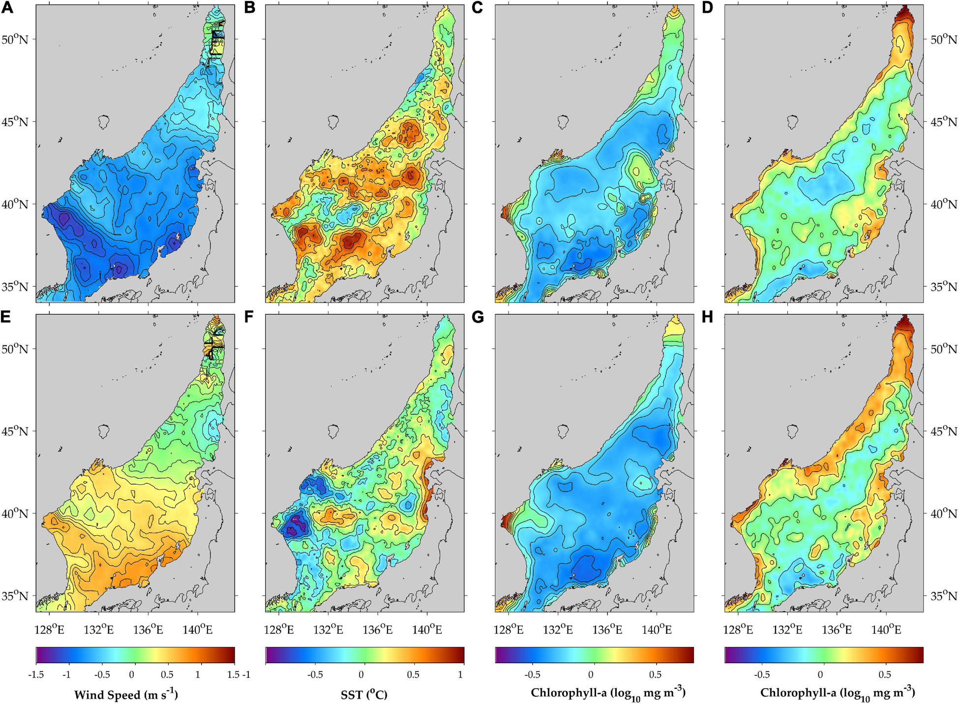
Figure 10. Spatial distributions of the (A) mean wind speed anomaly, (B) sea surface temperature (SST) anomaly, and (C) chlorophyll-a concentration (Chla) anomaly averaged over the periods of the positive AO index (> 1) in winter (December, January, and February) and (D) Chl-a anomaly in spring (March–May). (E–H) Are the same as (A–D) for the negative phase of AO (< -1).

The change in wind speed with respect to the change in AO can be identified by the histogram distribution as shown in Figure 11A. When the AO index is greater than + 1, the SST anomaly showed warming with positive values occupying 87.66% of the total area (Figure 10B). However, a negative AO produced opposite anomalies to those of the positive AO. The histogram of SST anomalies (Figure 11B) shows that there is an overall shift in the maximum frequency depending on the sign of the AO index. In particular, the coastal regions off the coast of North Korea showed strong negative SST anomalies (< -0.7°C) during the negative AO period (Figure 10F).

FIGURE 11

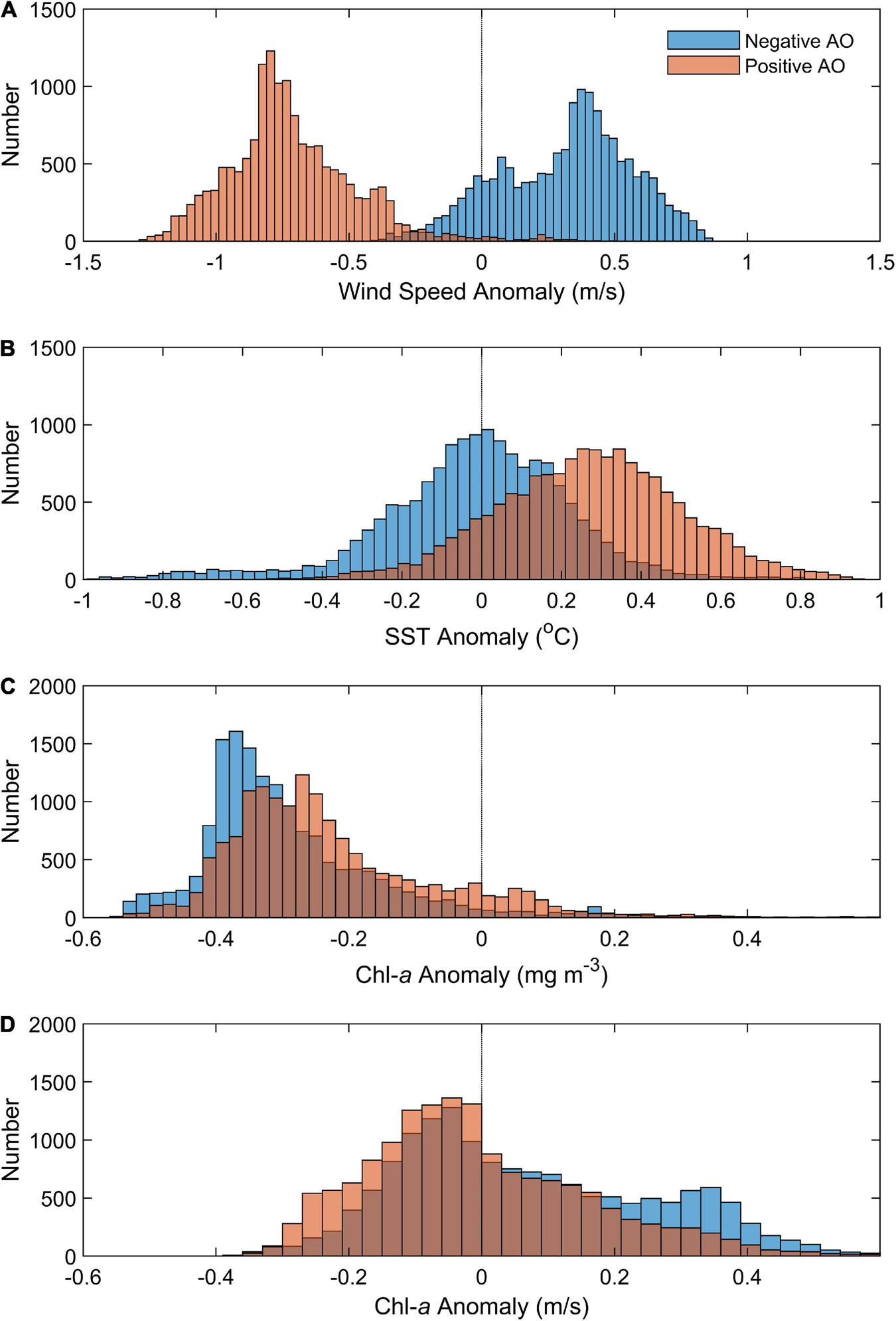
Figure 11. Histogram of the (A) wind speed anomaly, (B) sea surface temperature (SST) anomaly, and (C) chlorophyll-a concentration (Chl-a) anomaly averaged over the periods of the positive AO index (> 1) in winter (December, January, and February) and (D) Chl-a anomaly in spring (March–May).

Spatial Distribution of Chlorophyll-a Concentration During Winter Arctic Oscillation Periods

These SST and wind responses showed similar results to those of previous studies (He et al., 2017). In this study, the responses of the Chl-a concentration to the two phases of AO were analyzed. As a result of comparing Figures 10C,G, the chlorophyll concentrations during the positive AO phase were slightly higher than those during the negative AO phase. This seems to be related to relatively lower wind speed anomalies and warmer SSTs as shown in Figures 11A–C. In the case of a positive AO, 10% of the total area had positive Chl-a anomalies of approximately + 1 mg m^–3, and in the negative case, it was reduced to 4.8% of the total area. These results are consistent with our hypothesis. It could be possible that increased in wind speed alter the supply of nutrients, such as nitrates, phosphates, and silicates, to the surface layer before the onset of the spring bloom. These nutrients generally provide favorable conditions for phytoplankton photosynthesis. However, extremely strong winds have the opposite effects on the abundance of Chl-a concentration. They might deepen the mixed layer and suppress photosynthesis by reducing the number of photons in the surface layer (Park et al., 2020a). The northern part of the EJS has sufficient nutrients as it is relatively less stratified and well mixed vertically in winter. Thus, the positive AO phase might augment Chl-a responses. To examine whether this effect of AO variability persists through spring, long-term averages of Chl-a concentration values from March to May 2003–2020 are plotted for positive and negative AO indices in Figures 10D,H. However, the Chl-a concentration was conversely found to be more prosperous in spring when the AO was negative (Figures 10H, 11D). Thus, such immediate responses of the physical environment to the AO variations did not appear to last long until spring. Many other factors such as light conditions, stratification, nutrients, the entrainment process of the mixed layer, and other external forcing are presumed to interact with each other to derive the complicated spring bloom.

Spatial Distribution of Chlorophyll-a Concentration Responses to Arctic Oscillation Index Variations

Figure 12A shows the Chl-a response to the AO variations over the entire period, specifically β in Equation (5), regardless of a positive or negative phase. Most of the EJS showed a positive response to the Chl-a concentration, such as the northeastern part of the EJS, south of Vladivostok, and the Tsushima Warm Current regions. This means that Chl-a increases during positive AO periods. Conversely, a negative response exceeding -0.2 mg m^–3 appeared prominently in the North Korean coastal region. This suggests that in some small local regions there may be an opposite responses with decreasing (increasing) Chl-a concentrations during positive (negative) AO periods. In general, positive Chl-a responses occupying most of the EJS indicate possible links to low wind speeds during the positive AO phase.

FIGURE 12

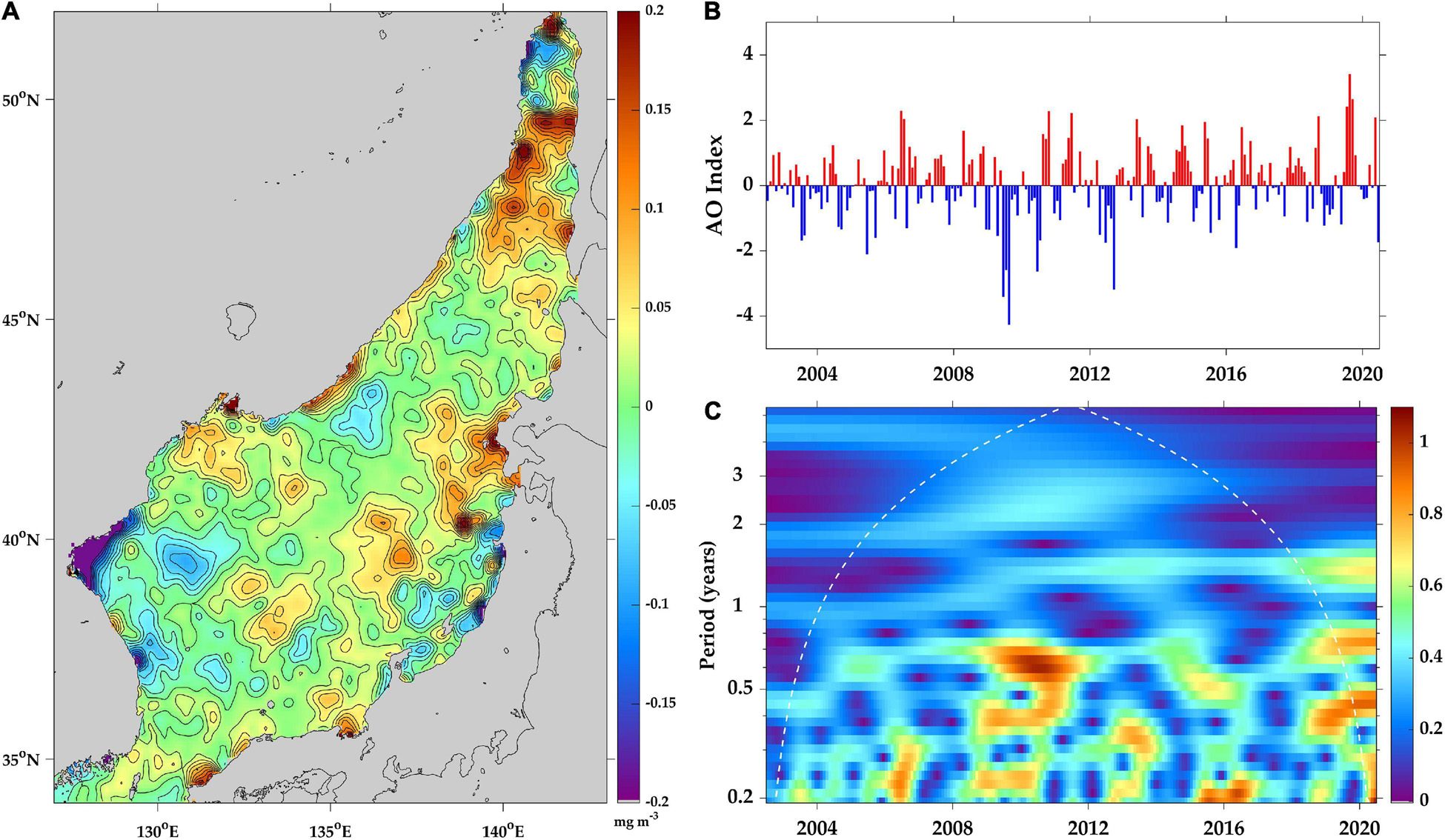
Figure 12. Spatial distribution of (A) response features of MODIS chlorophyll-a concentration variations to the Arctic Oscillation (AO) index in the East Sea (Sea of Japan), (B) AO index time series, and (C) wavelets of AO index variations from 2003 to 2020.

Since there are various mesoscale eddies and warm and cold currents under a complicated environment in the EJS (Figure 1), the spatial response of Chl-a to AO might appear with various spatial structures. It could also be attributed to the strong temporal variability of the AO. As shown in Figure 12B, the AO index exhibited high variability over time. Significantly negative AO index values (-4 to -3) were observed in February 2010 and again in March 2013. In contrast, there were high positive AO indices as peaks in December 2007, April 2013, and February 2020. As a result of analyzing the wavelet of this AO index, most of the AO fluctuations were found to be limited to short periods of less than 1 year (Figure 12C). In particular, the inter-annual fluctuations were very large, as was the case when high spectral energy of AO index variability emerged in 2011. Despite the complicate spatial structure, the Chl-a responses to the AO variations had similar directionality depending on the AO signs (Figure 12A).

Spatial Distribution of Chlorophyll-a Response to El Niño-Southern Oscillation

Sea Surface Temperature Distribution During El Niño and La Niña Periods in Summer

The ENSO has a profound impact on not only the global oceans but also regional seas. It influences the interannual variations of physical environment in the local seas through oceanic and atmospheric interactions, which is expected to eventually affect biological Chl-a concentration responses during ENSO periods. In the EJS, the ENSO affects the various environment, especially in summer and winter rather than spring. Therefore, in this study, we focused on the ENSO-induced SST change in summer, avoiding the winter change in which AO index variations are dominant.

First of all, we investigated the SST anomalies of the EJS during summer (June, July, and August) with absolute ENSO indices (| MEI| > 1). Figure 13A shows the spatial pattern of the SST anomalies during the El Niño events in summer (June–August). More than half of regions (54.75%) had negative anomalies down to -1.5°C over extensive areas of the southwest and northeast EJS. There are weakly positive SST anomalies of approximately 0.5–1.0°C in the near-coastal region of the Primorye, the northern Tatar Strait, and the Yamato Basin. However, during the La Niña period, the SST anomaly had a maximum of 1.5°C and was positive in most regions of the EJS, accounting for 90.94% of the total area (Figure 13B). Large positive anomalies of 1°C or more were distributed in the vicinity of 134°E north of the SPF along a latitude of 40°N. During El Niño events in the summer, the SST anomalies of the EJS were inversely proportional to those of La Niña (Figure 14C). That is, as the SST decreased, the Chl concentration showed a tendency to conversely increase with a rate of -0.012 mg m^–3°C (p-value = 0.0010). This distinct difference in the SST environment between El Niño and La Niña in summer is expected to influence changes in the Chl-a variations.

FIGURE 13

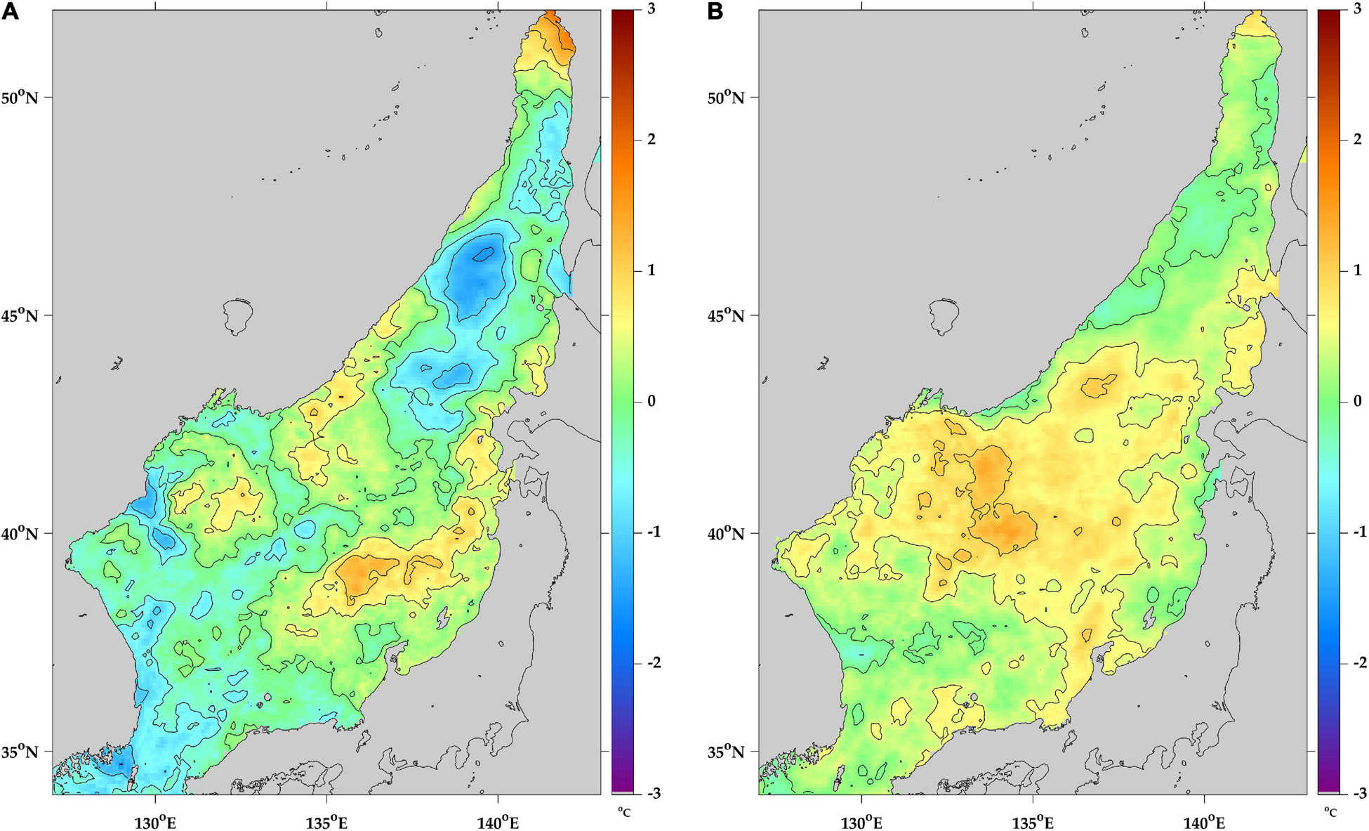
Figure 13. Spatial distribution of sea surface temperature anomalies averaged for the periods of (A) El Niño (ENSO index > 1) and (B) La Niña (ENSO index < -1) in the East Sea (Sea of Japan) in summer (June–August) from 2003 to 2020.

FIGURE 14

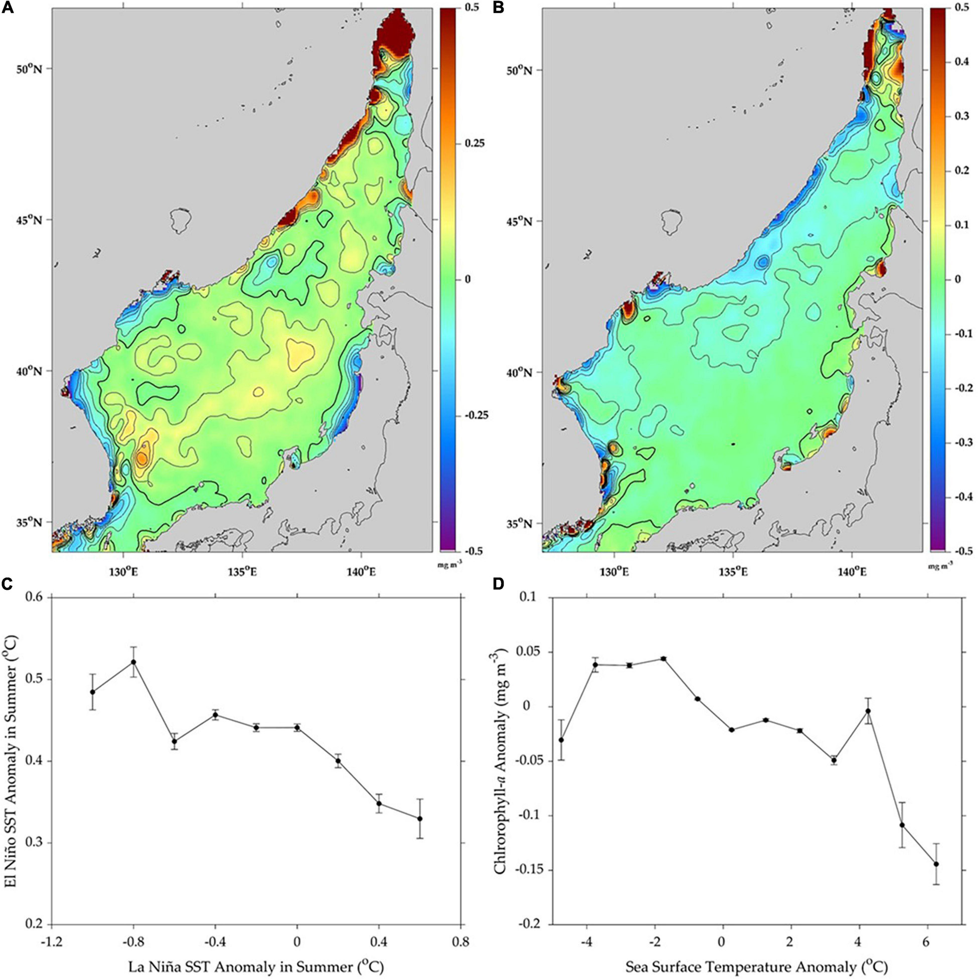
Figure 14. Spatial distributions of MODIS chlorophyll-a concentration anomalies averaged for the periods of (A) El Niño (ENSO index > 1) and (B) La Niña (ENSO index < -1) in the East Sea (Japan Sea) in summer (June–August) from 2003 to 2020. (C) Sea surface temperature anomalies (SSTA) during El Niño (ENSO index > 1) against SSTA during La Niña (ENSO index < 1) in the entire region of the East Sea (Japan Sea) in summer (June–August) from 2003 to 2020 and (D) chlorophyll-a concentration anomaly as a function of the SST anomaly for high amplitude (|MEI|> 1) ENSO periods for the same period of (C). Error bars represent the mean error ($\mathrm{\sigma }/\sqrt{N-1}$, σ: standard deviation, N: the data number) within a given interval.

Chlorophyll-a Concentration Distribution During El Niño-Southern Oscillation Periods in Summer

To investigate the overall relationship between SSTA and Chl-a anomaly patterns during ENSO periods, we derived the temporal means of the Chl-a anomalies for both El Niño and La Niña periods. Figure 14 shows the means of the Chl-a anomalies based on the high amplitudes of MEI indices during the El Niño (> 1) and La Niña (< -1) periods, respectively. During the El Niño period in summer, the Chl-a anomaly showed positive values in the entire EJS and enhanced local Chl-a increase along the Primorye Coast (> 45°N), amounting to 0.5 mg m^–3, and in the southwestern part at lower latitudes < 38°N (Figure 14A). Most areas (76.78%) showed positive responses. During El Niño events, negative responses of Chl-a appeared along the coasts of the Korean Peninsula, coastal region of Japan, and west of Sakhalin Island. Except for these coastal areas of the EJS, the positive responses were predominant in most central areas.

On the other hand, the Chl-a anomalies in response to the La Niña events with MEI < -1 yielded relatively negative values and lower amplitudes than those during the El Niño period. During the La Niña period, Chl-a increased only in 11.66% grids of the total area, and most areas in the central part of the EJS showed a weak negative response about -0.2 mg m^–3 (Figure 14B). In the Russian coast, there were negative responses as opposed to positive responses during the El Niño period. Opposite responses with different signs were detected at the coastal upwelling region at 35–37°N latitudes off the southeastern coast of Korea. This region is well known for coastal upwelling with significantly low SST differences > 15°C from ambient sea waters. This phenomenon was induced by southerly or southeasterly winds at the southeast coastal region in summer (Figure 9). The wind field varied widely in terms of speed and direction in July. This wind field and its associated upwelling provide nutrient-rich cold waters near the surface and result in Chl-a bloom (Byun and Seung, 1984; Lee and Na, 1985; Yoo and Park, 2009; Park and Kim, 2010; Kim et al., 2014).

Figure 14D supports this relationship between the Chl-a response and the SST anomaly in summer during the El Niño/La Niña periods. The Chl-a anomaly variations were negatively correlated with the SST anomaly changes induced by ENSO variability during dominant ENSO events (for | MEI| > 1). These features coincide with the SSTA and Chl-a distributions shown in Figures 13, 14. The overall linear tendency implies the role of SST anomalies in the responses of Chl-a during ENSO events. As the SST decreased, the Chl concentration tended to increase in an inverse rate of -0.012 mg m^–3°C (p-value = 0.0054). The correlated responses indicate the effects of SST anomalies on Chl-a variability in summer during ENSO periods.

Spatial Distribution of Chlorophyll-a Concentration Responses to El Niño-Southern Oscillation Index Variations

Figure 15A shows the spatial distributions of Chl-a responses expressed by the coefficient α in Equation (5) as the responses of Chl-a to ENSO index variability, regardless of the season and magnitude of ENSO. Most of the responses were in the range of -0.2 to 0.2 mg m^–3 relative to the ENSO index (-2.43 to 2.21), as shown in Figure 15B. The time series of the MEI index had high interannual variations at frequencies longer than 1 year, as shown in the wavelets (Figure 15C), which was quite different from the wavelets with intra-seasonal periods of AO index variations presented in Figure 12C.

FIGURE 15

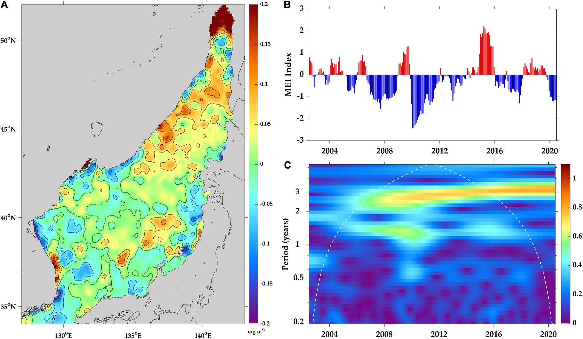
Figure 15. Spatial distribution of (A) the responses of MODIS chlorophyll-a concentration variations to the ENSO index in the East Sea (Japan Sea) for 2003–2020, (B) ENSO index time series, and (C) wavelet of the ENSO index variations.

In more than half of the EJS area (58.71%), the Chl-a concentration showed a positive response to the positive ENSO index (Figure 15A). In particular, the positive responses were widely distributed in the northeastern part of the EJS. This means that this region produced increased Chl-a concentrations during the El Niño period. In contrast, this region tended to give rise to decreased Chl-a during the La Niña period with increased SST warming in summer. Positive responses of 0.2 mg m^–3 were also found along the central coast of the southern Korean Peninsula where upwelling occurred every summer. Relatively cooler SSTs might contribute to positive Chl-a blooms by reducing stratification that is favorable for the nutrient supply under oligotrophic conditions in summer. However, the opposite negative response could be also observed in the western part of the EJS with a lower Chl-a concentration in the coastal regions during El Niño events.

Potential Causes and Further Study on the Trend in Chlorophyll-a Concentrations

In this study, we investigated the response pattern of Chl-a concentration variability to the climate index using multivariate regression. We considered long-term trends and multifrequency variations in Chl-a concentrations. However, other factors affect the temporal variability of Chl-a concentrations in the EJS including mixed layer depth, SSW forcing, wind mixing, Ekman pumping and transport, euphotic layer and vertical stratification, and surface currents (Kim et al., 2000; Yoo and Kim, 2004; Onitsuka and Yanagi, 2005; Park et al., 2006, 2014; Onitsuka et al., 2010). Atmospheric and oceanic conditions generate an integrated physical environment contributing to variability in Chl-a concentrations. In addition, the dynamics of nitrate and phosphate supply to the euphotic layer play key roles in phytoplankton growth. Combined environments influence Chl-a blooms through physical and biogeochemical processes. Details of the relationships between Chl-a concentration variability and physical forcing in the EJS have already been presented and discussed in other studies (e.g., Yamada et al., 2004; Yamada and Ishizaka, 2006; Park et al., 2020a).

This study presented Chl-a concentration variability in terms of two representative climate indices and long-term trends. The detailed physio-biogeochemical processes involved in its cause require further investigation. The EJS has been subjected to dynamic atmospheric changes from AO variations in the polar region. Hence, the temporal variations in Chl-a should reflect changes consistent with recent Arctic warming. The present study focused on long-term trends and their relationships with two representative climate indices. These associations have seldom been examined in previous studies, especially in terms of their spatial distributions. The response patterns of Chl-a concentration distribution to AO and ENSO variability might help to clarify Chl-a concentration dynamics and spatial distribution in response to climate change. Recently, the central Pacific type of ENSOs have increased in frequency and could affect the variability of atmospheric and oceanic conditions and low-level marine ecosystems in the regional seas (Yeh et al., 2009; Lee and McPhaden, 2010). However, this study did not divide the ENSOs because of the relatively weak responses of variability in Chl-a concentrations in the mid-latitude region and relatively short period of the satellite Chl-a database. For this reason, the present study focused on the features of Chl-a variations in summer when the physical environmental changes were dominant between El Niño and La Niña periods. Future studies should analyze more detailed linkage processes based on extensive in situ observations in the EJS.

Conclusion

In this study, temporal changes in chlorophyll concentrations were understood by dividing them into seasonal and intraseasonal seasonal variations, AO and ENSO index variations, and long-term trends in Chl-a concentrations by multivariate regression. The interannual variations in Chl-a concentrations in the EJS were much higher than the seasonal variations. Chl-a concentrations have been increased throughout the EJS over the past 18 years (2003–2020), especially north of the SPF. This trend is markedly different from the trends revealed in previous studies on the magnitude and spatial distribution of Chl-a concentrations. It is inferred that the recent changes in the Arctic Ocean had a significant effect on Chl-a variability. This study also revealed that the wind speed and SST of the EJS responded oppositely according to the sign of the AO index, which have led to eventual Chl-a responses. In particular, the SSWs tended to increase in the northeastern part of the EJS. Analysis of the wind vector trend showed that the northerly wind components have been strengthened, and the westerly winds were intensified off the eastern coast of the Korean Peninsula as well. There was an inverse correlation between the SST anomaly and Chl-a concentration anomaly of the EJS in summer during El Niño and La Niña periods. This was confirmed as the ENSO index variability affected the interannual variation in chlorophyll concentrations in the EJS. As a result of analyzing long-term trends along with seasonal changes in Chl-a concentration variability in the EJS, this study showed that climate index variability in the equatorial Pacific and Arctic oceans affected the low-level ecosystems of the local seas through an ocean–atmospheric connection. For a more in-depth understanding of Chl-a variability, a longer period of satellite data is needed to investigate the relationship between the Chl-a responses and the physical environment and to perform a more comprehensive analysis by considering other climate indices.

Data Availability Statement

The original contributions presented in the study are included in the article/supplementary material, further inquiries can be directed to the corresponding author/s.

Author Contributions

K-AP conceptualized, organized, analyzed the datasets, prepared all figures, and wrote the manuscript. J-EP synthesized the data, re-tuned and further-developed the algorithm of chlorophyll-a data composites. C-KK revised the manuscript and funded this study. All authors contributed to the final version of the manuscript.

Funding

This work has been carried out as part of “Deep Water Circulation and Material Cycling in the East Sea (20160040)” funded by the Ministry of Oceans and Fisheries, Korea. Multi-satellite data processing was supported in part by the National Research Foundation of Korea (NRF), grant funded by the Korean Government (MSIT) (No. 2020R1A2C2009464). C-KK was partly supported by the project titled “Long-term change of structure and function in marine ecosystems of Korea.”

Conflict of Interest

The authors declare that the research was conducted in the absence of any commercial or financial relationships that could be construed as a potential conflict of interest.

Publisher’s Note

All claims expressed in this article are solely those of the authors and do not necessarily represent those of their affiliated organizations, or those of the publisher, the editors and the reviewers. Any product that may be evaluated in this article, or claim that may be made by its manufacturer, is not guaranteed or endorsed by the publisher.

Acknowledgments

NOAA High Resolution SST data provided by the NOAA/OAR/ESRL PSL, Boulder, Colorado, United States, from their Web site at https://psl.noaa.gov. The authors thank NASA GSFC (https://oceancolor.gsfc.nasa.gov) for providing MODIS chlorophyll-a concentration data.

Footnotes

1. ^ https://oceancolor.gsfc.nasa.gov/
2. ^ https://www.psl.noaa.gov/enso/mei/

References

Alvain, S., Moulin, C., Dandonneau, Y., and Loisel, H. (2008). Seasonal distribution and succession of dominant phytoplankton groups in the global ocean: a satellite view. Global Biogeochem. Cycles 22:GB3001. doi: 10.1029/2007GB003154

CrossRef Full Text | Google Scholar

Baker, A. C., Starger, C. J., McClanahan, T. R., and Glynn, P. W. (2004). Corals’ adaptive response to climate change. Nature 430:741. doi: 10.1038/430741a

PubMed Abstract | CrossRef Full Text | Google Scholar

Behrenfeld, M. J., O’Malley, R. T., Boss, E. S., Westberry, T. K., Graff, J. R., Halsey, K. H., et al. (2016). Revaluating ocean warming impacts on global phytoplankton. Nat. Clim. Change 6, 323–330. doi: 10.1038/nclimate2838

CrossRef Full Text | Google Scholar

Bindoff, N. L., Cheung, W. W. L., Kairo, J. G., Arístegui, J., Guinder, V. A., Hallberg, R., et al. (2019). “Changing ocean, marine ecosystems, and dependent communities,” in IPCC Special Report on the Ocean and Cryosphere in a Changing Climate, eds H.-O. Pörtner, D. C. Roberts, V. Masson-Delmotte, P. Zhai, M. Tignor, E. Poloczanska, et al. (Geneva: IPCC), 447–588. doi: 10.1017/9781009157964.007

CrossRef Full Text | Google Scholar

Bonjean, F., and Lagerloef, G. S. (2002). Diagnostic model and analysis of the surface currents in the tropical Pacific Ocean. J. Phys. Oceanogr. 32, 2938–2954. doi: 10.1175/1520-0485(2002)032<2938:dmaaot>2.0.co;2

CrossRef Full Text | Google Scholar

Bulgin, C. E., Merchant, C. J., and Ferreira, D. (2020). Tendencies, variability and persistence of sea surface temperature anomalies. Sci. Rep. 10:7986. doi: 10.1038/s41598-020-64785-9

PubMed Abstract | CrossRef Full Text | Google Scholar

Byun, S. -K., and Seung, Y. H. (1984). “Description of current structure and coastal upwelling in the southwest Japan sea—summer 1981 and spring 1982,” in Ocean Hydrodynamics of the Japan and East China Seas, ed. T. Ichiye (Amsterdam: Elsevier Oceanography Series), 83–93. doi: 10.1016/s0422-9894(08)70293-9

CrossRef Full Text | Google Scholar

Campbell, J. W., Blaisdell, J. M., and Darzi, M. (1995). Level-3 SeaWiFS data products: spatial and temporal binning algorithms. NASA Tech. Memo. 32, 1–73. doi: 10.1145/3473006

CrossRef Full Text | Google Scholar

Choi, B. H., Kim, D. H., and Fang, Y. (1999). Tides in the East Asian Seas form a fine-resolution global ocean tidal model. Mar. Technol. Soc. J. 33:36. doi: 10.4031/mtsj.33.1.5

CrossRef Full Text | Google Scholar

Church, J. A., Clark, P. U., Cazenave, A., Gregory, J. M., Jevrejeva, S., Levermann, A., et al. (2013). “Sea level change,” in Climate Change 2013: The Physical Science Basis. Contribution of Working Group I to the Fifth Assessment Report of the Intergovernmental Panel on Climate Change, eds T. F. Stocker, D. Qin, G.-K. Plattner, M. Tignor, S. K. Allen, J. Boschung, et al. (Cambridge: Cambridge University Press).

Google Scholar

Doney, S. C., Ruckelshaus, M., Emmett Duffy, J., Barry, J. P., Chan, F., English, C. A., et al. (2012). Climate change impacts on marine ecosystems. Annu. Rev. Mar. Sci. 4, 11–37.

Google Scholar

Donlon, C. J., Martin, M., Stark, J., Roberts-Jones, J., Fiedler, E., and Wimmer, W. (2012). The operational sea surface temperature and sea ice analysis (OSTIA) system. Remote Sens. Environ. 116, 140–158. doi: 10.1007/s13143-018-0050-y

PubMed Abstract | CrossRef Full Text | Google Scholar

Dutkiewicz, S., Hickman, A. E., Jahn, O., Henson, S., Beaulieu, C., and Monier, E. (2019). Ocean colour signature of climate change. Nat. Commun. 10:578. doi: 10.1038/s41467-019-08457-x

PubMed Abstract | CrossRef Full Text | Google Scholar

Dutkiewicz, S., Scott, J. R., and Follows, M. J. (2013). Winners and losers: ecological and biogeochemical changes in a warming ocean. Global Biogeochem. Cycles 27, 463–477. doi: 10.1002/gbc.20042

CrossRef Full Text | Google Scholar

Fisher, R. (1918). Studies in crop variation. I. An examination of the yield of dressed grain from Broadbalk. J. Agric. Sci. 11, 107–135. doi: 10.1017/s0021859600003750

CrossRef Full Text | Google Scholar

Frenger, I., Gruber, N., Knutti, R., and Münnich, M. (2013). Imprint of southern ocean eddies on winds, clouds and rainfall. Nat. Geosci. 6, 608–612. doi: 10.1038/ngeo1863

CrossRef Full Text | Google Scholar

Gamo, T. (2011). Dissolved oxygen in the bottom water of the Sea of Japan as a sensitive alarm for global climate change. TrAC Trends Anal. Chem. 30, 1308–1319. doi: 10.1016/j.trac.2011.06.005

CrossRef Full Text | Google Scholar

Garcia-Eidell, C., Comiso, J. C., Berkelhammer, M., and Stock, L. (2021). Interrelationships of sea surface salinity, chlorophyll-α concentration, and sea surface temperature near the Antarctic ice edge. J. Clim. 34, 6069–6086.

Google Scholar

Gaube, P., Chelton, D. B., Strutton, P. G., and Behrenfeld, M. J. (2013). Satellite observations of chlorophyll, phytoplankton biomass, and Ekman pumping in nonlinear mesoscale eddies. J. Geophys. Res. Oceans 118, 6349–6370. doi: 10.1002/2013JC009027

CrossRef Full Text | Google Scholar

Gohin, F., Van der Zande, D., Tilstone, G., Eleveld, M. A., Lefebvre, A., Andrieux-Loyer, F., et al. (2019). Twenty years of satellite and in situ observations of surface chlorophyll-a from the northern Bay of Biscay to the eastern English channel. Is the water quality improving? Remote Sens. Environ. 233:111343. doi: 10.1016/j.rse.2019.111343

CrossRef Full Text | Google Scholar

Gregg, W. W., Conkright, M. E., Ginoux, P., O’Reilly, J. E., and Casey, N. W. (2003). Ocean primary production and climate: global decadal changes. Geophys. Res. Lett. 30:1809.

Google Scholar

Hammond, M. L., Beaulieu, C., Henson, S. A., and Sahu, S. K. (2020). Regional surface chlorophyll trends and uncertainties in the global ocean. Sci. Rep. 10:15273. doi: 10.1038/s41598-020-72073-9

PubMed Abstract | CrossRef Full Text | Google Scholar

He, S., Gao, Y., Li, F., Wang, H., and He, Y. (2017). Impact of arctic oscillation on the East Asian climate: a review. Earth Sci. Rev. 164, 48–62. doi: 10.1016/j.earscirev.2016.10.014

CrossRef Full Text | Google Scholar

Hyun, J. H., Kim, D., Shin, C. W., Noh, J. H., Yang, E. J., Mok, J. S., et al. (2009). Enhanced phytoplankton and bacterioplankton production coupled to coastal upwelling and an anticyclonic eddy in the Ulleung Basin, East Sea. Aquat. Microb. Ecol. 54, 45–54. doi: 10.3354/ame01280

CrossRef Full Text | Google Scholar

Ichiye, T. (1984). “Some problems of circulation and hydrography of the Japan Sea and the Tsushima Current,” in Ocean Hydrodynamics of the Japan and East China Seas, Elsevier Oceanogr. Ser, Vol. 39, ed. T. Ichiye (New York, NY: Elsevier), 15–54. doi: 10.1016/s0422-9894(08)70289-7

CrossRef Full Text | Google Scholar

Jo, C. O., Park, S., Kim, Y. H., Park, K.-A., Park, J. J., Park, M. K., et al. (2014). Spatial distribution of seasonality of SeaWiFS chlorophyll-a concentrations in the East/Japan Sea. J. Mar. Syst. 139, 288–298. doi: 10.1016/j.jmarsys.2014.07.004

CrossRef Full Text | Google Scholar

Kim, H.-C., Yoo, S. J., and Oh, I. S. (2007). Relationship between phytoplankton bloom and wind stress in the sub-polar frontal area of the Japan/East Sea. J. Mar. Syst. 67, 205–216. doi: 10.1016/j.jmarsys.2006.05.016

CrossRef Full Text | Google Scholar

Kim, K., Kim, K. R., Min, D. H., Volkov, Y., Yoon, J. H., and Takematsu, M. (2001). Warming and structural changes in the East (Japan) Sea: a clue to future changes in global oceans? Geophys. Res. Lett. 28, 3293–3296. doi: 10.1029/2001gl013078

CrossRef Full Text | Google Scholar

Kim, S. W., Saitoh, S., Ishizaka, J., Isoda, Y., and Kishino, M. (2000). Temporal and spatial variability of phytoplankton pigment concentration in the Japan Sea derived from CZCS images. J. Oceanogr. 56, 527–538.

Google Scholar

Kim, T. S., Park, K.-A., Li, X., and Hong, S. (2014). SAR-derived wind fields at the coastal region in the East/Japan Sea and relation to coastal upwelling. Int. J. Remote Sens. 35, 3947–3965. doi: 10.1080/01431161.2014.916438

CrossRef Full Text | Google Scholar

Kouketsu, S., Kaneko, H., Okunishi, T., Sasaoka, K., Itoh, S., Inoue, R., et al. (2015). Mesoscale eddy effects on temporal variability of surface chlorophyll a in the Kuroshio extension. J. Oceanogr. 72, 439–451. doi: 10.1007/s10872-015-0286-4

CrossRef Full Text | Google Scholar

Kubryakov, A., Stanichny, S., and Zatsepin, A. (2016). River plume dynamics in the Kara Sea from altimetry-based lagrangian model, satellite salinity and chlorophyll data. Remote Sens. Environ. 176, 177–187. doi: 10.1016/j.rse.2016.01.020

CrossRef Full Text | Google Scholar

Laws, E. A., and Bannister, T. T. (1980). Nutrient- and light-limited growth of Thalassiosira fluviatilis in continuous culture, with implications for phytoplankton growth in the ocean. Limnol. Oceanogr. 25, 457–473. doi: 10.4319/lo.1980.25.3.0457

CrossRef Full Text | Google Scholar

Lee, E.-Y., and Park, K.-A. (2019). Change in the recent warming trend of sea surface temperature in the East Sea (Sea of Japan) over decades (1982–2018). Remote Sens. 11:2613. doi: 10.3390/rs11222613

CrossRef Full Text | Google Scholar

Lee, J. C., and Na, J. Y. (1985). Structure of upwelling off the southeast coast of Korea. J. Oceanol. Soc. Korea 20, 6–19.

Google Scholar

Lee, S. H., Son, S., Dahms, H. U., Park, J. W., Lim, J. H., Noh, J. H., et al. (2014). Decadal changes of phytoplankton chlorophyll-a in the East Sea/Sea of Japan. Oceanology 54, 771–779. doi: 10.1134/s0001437014060058

CrossRef Full Text | Google Scholar

Lee, T., and McPhaden, M. J. (2010). Increasing intensity of El Niño in the central-equatorial Pacific. Geophys. Res. Lett. 37:L14603.

Google Scholar

Li, W., El-Askary, H., Qurban, M. A., Proestakis, E., Garay, M. J., Kalashnikova, O. V., et al. (2018). An assessment of atmospheric and meteorological factors regulating Red Sea phytoplankton growth. Remote Sens. 10:673. doi: 10.3390/rs10050673

CrossRef Full Text | Google Scholar

Liu, M., Liu, X., Ma, A., Li, T., and Du, Z. (2014). Spatio-temporal stability and abnormality of chlorophyll-a in the northern South China sea during 2002-2012 from MODIS images using wavelet analysis. Cont. Shelf Res. 75, 15–27. doi: 10.1016/j.csr.2013.12.010

CrossRef Full Text | Google Scholar

Martin, A. P., and Richards, K. J. (2001). Mechanisms for vertical nutrient transport within a North Atlantic mesoscale eddy. Deep Sea Res. II Top. Stud. Oceanogr. 48, 757–773. doi: 10.1016/s0967-0645(00)00096-5

CrossRef Full Text | Google Scholar

May, C. L., Koseff, J. R., Lucas, L. V., Cloern, J. E., and Schoellhamer, D. H. (2003). Effects of spatial and temporal variability of turbidity on phytoplankton blooms. Mar. Ecol. Prog. Ser. 254, 111–128. doi: 10.1073/pnas.032206999

PubMed Abstract | CrossRef Full Text | Google Scholar

McClain, C. R. (2009). A decade of satellite ocean color observations. Annu. Rev. Mar. Sci. 1, 19–42. doi: 10.1146/annurev.marine.010908.163650

PubMed Abstract | CrossRef Full Text | Google Scholar

McGillicuddy, D. J., Anderson, L. A., Bates, N. R., Bibby, T., Buesseler, K. O., Carlson, C. A., et al. (2007). Eddy/wind interactions stimulate extraordinary mid-ocean plankton blooms. Science 316, 1021–1026. doi: 10.1126/science.1136256

PubMed Abstract | CrossRef Full Text | Google Scholar

Mobley, C. D., Stramski, D., Bisset, W. P., and Boss, E. (2004). Optical modeling of ocean waters: is the case-1 case-2 still useful? Oceanography 17, 60–67. doi: 10.5670/oceanog.2004.48

CrossRef Full Text | Google Scholar

National Oceanic and Atmospheric Administration [NOAA] (2016). Extended Reconstructed Sea Surface Temperature (ERSST.v4). National Centers for Environmental Information. Available Online at: www.ncdc.noaa.gov/data-access/marineocean-data/extended-reconstructed-sea-surface-temperature-ersst [accessed October 2021].

Google Scholar

Olhede, S., and Walden, A. (2002). Generalized morse wavelets. IEEE Trans. Signal Process. 50, 2661–2670. doi: 10.1109/tsp.2002.804066

CrossRef Full Text | Google Scholar

Onitsuka, G., Miyahara, K., Hirose, N., Watanabe, S., Semura, H., Hori, R., et al. (2010). Large-scale transport of Cochlodinium polykrikoides blooms by the Tsushima warm current in the southwest Sea of Japan. Harmful Algae 9, 390–397. doi: 10.1016/j.hal.2010.01.006

CrossRef Full Text | Google Scholar

Onitsuka, G., and Yanagi, T. (2005). Differences in ecosystem dynamics between the northern and southern parts of the Japan Sea: analyses with two ecosystem models. J. Oceanogr. 61, 415–433. doi: 10.1007/s10872-005-0051-1

CrossRef Full Text | Google Scholar

Park, J.-E., Park, K.-A., Kang, C.-K., and Kim, G. (2020a). Satellite-observed chlorophyll-a concentration variability and its relation to physical environmental changes in the East Sea (Japan Sea) from 2003 to 2015. Estuar. Coasts 43, 630–645. doi: 10.1007/s12237-019-00671-6

CrossRef Full Text | Google Scholar

Park, J.-E., Park, K.-A., Kang, C.-K., and Park, Y. J. (2020b). Short-term response of chlorophyll-a concentration to change in sea surface wind field over mesoscale eddy. Estuar. Coasts 43, 646–660. doi: 10.1007/s12237-019-00643-w

CrossRef Full Text | Google Scholar

Park, J.-E., Park, K.-A., Ullman, D. S., Cornillon, P. C., and Park, Y. J. (2016). Observation of diurnal variations in mesoscale eddy sea-surface currents using GOCI data. Remote Sens. Lett. 7, 1131–1140. doi: 10.1080/2150704x.2016.1219423

CrossRef Full Text | Google Scholar

Park, K., and Chung, J. Y. (1999). Spatial and temporal scale variations of sea surface temperature in the East Sea using NOAA/AVHRR data. J. Oceanogr. 55, 271–288.

Google Scholar

Park, K.-A., Chung, J., and Kim, K. (2004). Sea surface temperature fronts in the East (Japan) Sea and temporal variations. Geophys. Res. Lett. 31:L07304.

Google Scholar

Park, K.-A., Kang, C.-K., Kim, K.-R., and Park, J.-E. (2014). Role of sea ice on satellite-observed chlorophyll-a concentration variations during spring bloom in the East/Japan sea. Deep Sea Res. I Oceanogr. Res. Pap. 83, 34–44. doi: 10.1016/j.dsr.2013.09.002

CrossRef Full Text | Google Scholar

Park, K.-A., Kim, K., Cornillon, P. C., and Chung, J. Y. (2006). Relationship between satellite-observed cold water along the Primorye coast and sea ice in the East Sea (the Sea of Japan). Geophys. Res. Lett. 33:L10602. doi: 10.1016/j.dsr.2013.09.002

CrossRef Full Text | Google Scholar

Park, K. A., and Kim, K. R. (2010). Unprecedented coastal upwelling in the East/Japan Sea and linkage to long-term large-scale variations. Geophys. Res. Lett. 37:L09603. doi: 10.1029/2009GL042231

CrossRef Full Text | Google Scholar

Park, K. A., and Lee, E. Y. (2014). Semi-annual cycle of sea-surface temperature in the East/Japan Sea and cooling process. Int. J. Remote Sens. 35, 4287–4314. doi: 10.1080/01431161.2014.916437

CrossRef Full Text | Google Scholar

Park, K.-A., Park, J.-E., Choi, B.-J., Byun, D.-S., and Lee, E.-I. (2013). An oceanic current map of the east sea for science textbooks based on scientific knowledge acquired from oceanic measurements. J. Korean Soc. Oceanogr. 18, 234–265. doi: 10.7850/jkso.2013.18.4.234

PubMed Abstract | CrossRef Full Text | Google Scholar

Patti, B., Guisande, C., Bonanno, A., Basilone, G., Cuttitta, A., and Mazzola, S. (2010). Role of physical forcings and nutrient availability on the control of satellite-based chlorophyll a concentration in the coastal upwelling area of the Sicilian Channel. Sci. Mar. 74, 577–588. doi: 10.3989/scimar.2010.74n3577

PubMed Abstract | CrossRef Full Text | Google Scholar

Peloquin, J., Swan, C., Gruber, N., Vogt, M., Claustre, H., Ras, J., et al. (2013). The MAREDAT global database of high performance liquid chromatography marine pigment measurements. Earth Syst. Sci. Data 5, 109–123. doi: 10.5194/essd-5-109-2013

CrossRef Full Text | Google Scholar

Rivas, A. L., Dogliotti, A. I., and Gagliardini, D. A. (2006). Seasonal variability in satellite-measured surface chlorophyll in the Patagonian Shelf. Cont. Shelf Res. 26, 703–720. doi: 10.1016/j.csr.2006.01.013

CrossRef Full Text | Google Scholar

Schaeffer, B. A., Morrison, J. M., Kamykowski, D., Feldman, G. C., Xie, L., Liu, Y., et al. (2008). Phytoplankton biomass distribution and identification of productive habitats within the Galapagos Marine Reserve by MODIS, a surface acquisition system, and in-situ measurements. Remote Sens. Environ. 112, 3044–3054. doi: 10.1016/j.rse.2008.03.005

CrossRef Full Text | Google Scholar

Siegel, D. A., Behrenfeld, M. J., Maritorena, S., McClain, C. R., Antoine, D., Bailey, S. W., et al. (2013). Regional to global assessments of phytoplankton dynamics from the SeaWiFS mission. Remote Sens. Environ. 135, 77–91. doi: 10.1016/j.rse.2013.03.025

CrossRef Full Text | Google Scholar

Sloyan, B. M., Wanninkhof, R., Kramp, M., Johnson, G. C., Talley, L. D., Tanhua, T., et al. (2019). The global ocean ship-based hydrographic investigations program (GO-SHIP): a platform for integrated multidisciplinary ocean science. Front. Mar. Sci. 6:445. doi: 10.3389/fmars.2019.00445

CrossRef Full Text | Google Scholar

Son, S., Platt, T., Bouman, H., Lee, D., and Sathyendranath, S. (2006). Satellite observation of chlorophyll and nutrients increase induced by Typhoon Megi in the Japan/East Sea. Geophys. Res. Lett. 33:L05607.

Google Scholar

Thompson, D. W. J., and Wallace, J. M. (2000). Annular modes in the extratropical circulation. Part I: month-to-month variability. J. Clim. 13, 1000–1016. doi: 10.1175/1520-0442(2000)013<1000:amitec>2.0.co;2

CrossRef Full Text | Google Scholar

Verhoef, A., Portabella, M., and Stoffelen, A. (2012). High-resolution ASCAT scatterometer winds near the coast. IEEE Trans. Geosci. Remote Sens. 50, 2481–2487. doi: 10.1109/tgrs.2011.2175001

CrossRef Full Text | Google Scholar

Verspeek, J., Stoffelen, A., Verhoef, A., and Portabella, M. (2012). Improved ASCAT wind retrieval using NWP ocean calibration. IEEE Trans. Geosci. Remote Sens. 50, 2488–2494. doi: 10.1109/tgrs.2011.2180730

CrossRef Full Text | Google Scholar

Vogelzang, J., Stoffelen, A., Verhoef, A., and Figa-Saldaña, J. (2011). On the quality of high-resolution scatterometer winds. J. Geophys. Res. Oceans 116:C10033.

Google Scholar

Wang, Y., Jiang, H., Jin, J., Zhang, X. Y., Lu, X. H., and Wang, Y. Q. (2015). Spatial-temporal variations of Chlorophyll-a in the adjacent sea area of the Yangtze River estuary influenced by Yangtze River discharge. Int. J. Environ. Res. 12, 5420–5438. doi: 10.3390/ijerph120505420

PubMed Abstract | CrossRef Full Text | Google Scholar

Weatherhead, E. C., Reinsel, G. C., Tiao, G. C., Meng, X.-L., Choi, D., Cheang, W.-K., et al. (1998). Factors affecting the detection of trends: statistical considerations and applications to environmental data. J. Geophys. Res. 103, 17149–17161. doi: 10.1029/98jd00995

CrossRef Full Text | Google Scholar

Werdell, P. J., and Bailey, S. W. (2005). An improved in-situ bio-optical data set for ocean color algorithm development and satellite data product validation. Remote Sens. Environ. 98, 122–140. doi: 10.1016/j.rse.2005.07.001

CrossRef Full Text | Google Scholar

Wolter, K., and Timlin, M. S. (2011). El Niño/Southern Oscillation behaviour since 1871 as diagnosed in an extended multivariate ENSO index (MEI.ext). Int. J. Clim. 31, 1074–1087. doi: 10.1002/joc.2336

CrossRef Full Text | Google Scholar

Yamada, K., and Ishizaka, J. (2006). Estimation of interdecadal change of spring bloom timing, in the case of the Japan Sea. Geophys. Res. Lett. 33:L02608.

Google Scholar

Yamada, K., Ishzaka, J., Yoo, S., Kim, H.-C., and Chiba, S. (2004). Seasonal and interannual variability of sea surface chlorophyll a concentration in the Japan/East Sea (JES). Prog. Oceanogr. 61, 193–211. doi: 10.1016/j.pocean.2004.06.001

CrossRef Full Text | Google Scholar

Yamaguchi, H., Ishizaka, J., Siswanto, E., Son, Y. B., Yoo, S., and Kiyomoto, Y. (2013). Seasonal and spring interannual variations in satellite-observed chlorophyll-a in the Yellow and East China Seas: new datasets with reduced interference from high concentration of resuspended sediment. Cont. Shelf Res. 59, 1–9. doi: 10.1016/j.csr.2013.03.009

CrossRef Full Text | Google Scholar

Yamaguchi, H., Kim, H.-C., Son, Y. B., Kim, S. W., Okamura, K., Kiyomoto, Y., et al. (2012). Seasonal and summer interannual variations of SeaWiFS Chlorophyll-a in the Yellow Sea and East China Sea. Prog. Oceanogr. 105, 22–29. doi: 10.1016/j.pocean.2012.04.004

CrossRef Full Text | Google Scholar

Yeh, S.-W., Kug, J.-S., Dewitte, B., Kwon, M.-H., Kirtman, B. P., and Jin, F.-F. (2009). El Niño in a changing climate. Nature 461, 511–514. doi: 10.1038/nature08316

PubMed Abstract | CrossRef Full Text | Google Scholar

Yoo, S., and Kim, H.-C. (2004). Suppression and enhancement of the spring bloom in the Southwestern East Sea/Japan Sea. Deep Sea Res. II Top. Stud. Oceanogr. 51, 1093–1111. doi: 10.1016/s0967-0645(04)00102-x

CrossRef Full Text | Google Scholar

Yoo, S., and Park, J. (2009). Why is the southwest the most productive region of the East Sea/Sea of Japan? J. Mar. Syst. 78, 301–315. doi: 10.1016/j.jmarsys.2009.02.014

CrossRef Full Text | Google Scholar

Yu, Y., Xing, X., Liu, H., Yuan, Y., Wang, Y., and Chai, F. (2019). The variability of chlorophyll-a and its relationship with dynamic factors in the basin of the South China Sea. J. Mar. Syst. 200:103230. doi: 10.1016/j.jmarsys.2019.103230

CrossRef Full Text | Google Scholar

Zhang, Y., Huang, Z., Fu, D., Tsou, J. Y., Jiang, T., San Liang, X., et al. (2018). Monitoring of chlorophyll-a and sea surface silicate concentrations in the south part of Cheju island in the East China sea using MODIS data. Int. J. Appl. Earth Obs. Geoinf. 67, 173–178. doi: 10.1016/j.jag.2018.01.017

CrossRef Full Text | Google Scholar

Zhou, Q., Tian, L., Wai, O. W., Li, J., Sun, Z., and Li, W. (2018). Impacts of insufficient observations on the monitoring of short-and long-term suspended solids variations in highly dynamic waters, and implications for an optimal observation strategy. Remote Sens. 10:345. doi: 10.3390/rs10020345

CrossRef Full Text | Google Scholar