Impact of Mesoscale Circulation on the Structure of River Plumes During Large Rainfall Events Inshore of the East Australian Current

Estuarine outflow can have a significant impact on physical and ecological systems in the coastal ocean. Along southeastern Australia, inshore of the East Australian Current, the shelf is narrow, the coastal circulation is advection dominated, and river estuarine outflow tends to be low, hence river plumes have largely been ignored. For these reasons, we lack an understanding of the spatial and temporal evolution of river plumes during large rainfall events (which are projected to increase in frequency and intensity), and the interaction of the mesoscale circulation with the estuarine outflow remains to be explored. Using a high-resolution (750 m) hydrodynamic model, we simulate idealized plumes from 4 estuaries during three different mesoscale circulation scenarios and investigate the spatial and temporal evolution of the estuarine outflow under two contrasting rainfall events (normal and large). We explore the plume from the largest of the 4 rivers, the Hawkesbury River, to understand the impact of the mesoscale circulation. During the first EAC mode, the plume spreads both northward and southeastward. The offshore spread of the plume is the largest in this scenario (~12.5 km east of the river mouth) in the wet event. In the second EAC mode, this plume dispersal is toward the north and east, driven by the proximity of a cyclonic eddy on the shelf, with an eastward extension of 11 km. In the third EAC mode, most of this river plume spreads southward with some to the north, again dictated by the position of the cyclonic eddy. The cross-shelf dispersal is a minimum of 9.5 km from the river mouth. It takes around 6 days for the freshwater spatial extent of the plume in the wet event to return to the base case. These results show the importance of mesoscale EAC circulation on the shelf circulation when considering river plumes dispersal. Knowledge of the ultimate fate of riverborne material, dilution and cumulative effects will enable better environmental management of this dynamic region for the local government.

1. Introduction

Freshwater flow is a critical landscape process that influences the coastal marine ecosystems (Skreslet, 1986). River discharge stimulates phytoplankton and subsequently zooplankton assemblages by providing high nutrient concentrations (Schlacher et al., 2008). River plumes form biogeochemical hot spots in coastal seas worldwide and rank amongst the most productive regions of the world's oceans (Schlacher et al., 2008). Natural variation in freshwater flowing from rivers strongly influences the distribution and abundance of fish and invertebrates through changes in growth, survival, and recruitment (Gillson, 2011; Gillson et al., 2012). Freshwater flow is also a powerful forcing agent in coastal ecosystems (Schlacher et al., 2008). Freshwater flow has a pivotal role in determining fisheries production due to its effects on environmental conditions (Grimes, 2001; Lloret et al., 2004). Episodic flood events maintain and enhance biological productivity and modify the species composition of landings by altering rates of estuarine immigration and emigration due to changes in salinity altering habitat availability (Gillson, 2011). Gillson et al. (2012) showed that flood events can influence commercial fisheries by modifying landings composition, fishers' harvesting behavior, and revenue generation. Severe flood events cause widespread mortalities of fish due to the production of unfavorable water quality characteristics in estuarine and coastal systems, which have been documented in the Richmond, Clarence, and Mcleay River estuaries in eastern Australia (Dawson, 2002; Eyre et al., 2006; Kroon and Ludwig, 2010). Therefore, understanding the spatial and temporal evolution of river plumes, particularly during flood events, is an important issue in fisheries ecology.

It is recognized that the estuarine zone is an important site for physico-chemical processes (Covelli et al., 2007), where flood river plumes are important pathways for materials from terrestrial to the sea and dominant sources of coastal pollutants (Warrick et al., 2004). Jaffe et al. (1995) showed that the Tuy River plume effectively transports a variety of pollutants derived from anthropogenic activities, such as heavy metals and organic contaminants, into the coastal zone. By studying the chemical composition of suspended particulate matter, Kannan et al. (2012) identified the water masses and movement of Yangtze River plumes to the Yellow Sea in the transport of sediments and contaminants. The river discharge of wastewater which contains macronutrients and micropollutants, are known to cause various deleterious effects in the coastal environment (Lawrence, 2010). There is a growing need to understand the dispersion of river plumes across coastal marine systems, which is essential to drive catchment management actions in protecting our coastal environment.

The East Australian Current (EAC) a major western boundary current flows poleward along southeastern Australia and typically separates from the coast, between 31°S and 32.5°S (Cetina-Heredia et al., 2014). When the current separates, it typically sheds large anti-cyclonic eddies. Additionally, eddy dipoles can form, associated with cyclonic eddies (Malan et al., 2020). The cyclonic eddies either form as frontal eddies on the inside edge of the EAC jet (Roughan et al., 2017; Schaeffer et al., 2017) or as westward propagating cyclones that interact with the EAC jet (Roughan et al., 2017; Li et al., 2022).

The Hawkesbury Shelf region is located downstream of the EAC separation, which has been identified as a region of high productivity (Oke and Middleton, 2001). The shelf circulation in this region is dominated by three prominent circulation patterns, which are associated with the poleward along-shore flow of the EAC jet, the eddies and the eddy dipoles downstream of the typical EAC separation region (33°S) (Malan et al., 2020; Ribbat et al., 2020b; Roughan et al., 2022). The circulation modes are largely dictated by where the EAC separates and the presence (or absence) of anticyclonic and cyclonic eddies as described in Roughan et al. (2022). The three modes are shown clearly in the schematic diagram of Ribbat et al. (2020b), their Figure 12. While the circulation patterns have been studied in some detail, little is known about the impact of the mesoscale circulation over the Hawkesbury Shelf region. Moreover, this is the first study to explore the spatial and temporal evolution of the river plumes.

Most estuaries in the Hawkesbury Shelf region are drowned river valleys with strong oceanic influence. The rainfall is typically low with small river outflows, and their impacts have largely been neglected by many studies, for example, recent modeling studies of this region assume freshwater inflow is negligible (Kerry et al., 2016; Ribbat et al., 2020b). However, the river discharges dramatically increase during sporadic large rainfall events, which is three times larger than the mean inflow in the Hawkesbury River region (Gillson et al., 2012). In this case, their impact will become significant to coastal and shelf ecosystems.

Previous studies have used numerical models to trace the riverine freshwater by releasing dyes into the rivers in many coastal regions, such as the New York Bight (Zhang et al., 2010), the Rhine Region (Rijnsburger et al., 2021), the South Brazilian Bight (Marta-Almeida et al., 2021), the Yangtze River estuary (Yu et al., 2020; Wu et al., 2021), and the Great Barrier Reef (Colberg et al., 2020). Three-dimensional structure and evolution of the river plumes have been presented in these numerical simulations. However, the knowledge of the spatial and temporal evolution of river plumes in the Hawkesbury Shelf region is limited, especially with large river discharges during high rainfall events.

In this study, we use a high-resolution numerical model to understand the dilution of estuarine outflow during large rainfall events and the influence of the mesoscale circulation patterns on river plume structure inshore of the EAC. Section 2 describes the numerical model configuration and sensitivity experiments. The model simulations of the spatial and temporal evolution of the river plumes are presented in Section 3. In Sections 4, 5, we provide a further discussion and summary of the results.

2. Materials and Methods

2.1. Model Configuration

We use a series of nested configurations of the Regional Ocean Modeling System (ROMS) for the EAC system (Figure 1), building on configurations of Kerry and Roughan (2020); Li et al. (2021b, 2022); Ribbat et al. (2020b). ROMS is an open-source hydrodynamic model which is widely used (Shchepetkin and McWilliams, 2005) for coastal and shelf seas applications.

FIGURE 1

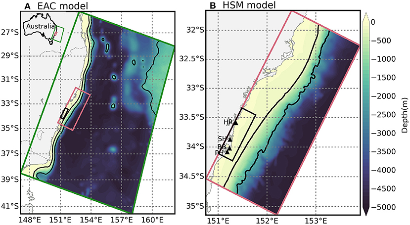
Figure 1. Schematic diagram showing the model bathymetry (color shading) in the study site along the east coast of Australia in the model domains. (A) The EAC-ROMS parent model, and (B) the nested HSM model. The locations of the 4 rivers are indicated by the black triangles: Hawkesbury River (HR), Sydney Harbor (SH), Botany Bay (BB), and Port Hacking (PH). The black rectangle indicates the region covers the plumes from the four rivers.

We use a high-resolution ROMS configuration of the Hawkesbury Shelf region, hereafter referred to as the Hawkesbury Shelf Model (HSM) model, with a model domain is shown in Figure 1B. The HSM model has a horizontal resolution of 750 × 750 m (Ribbat et al., 2020a,b) and 30 vertical s-layers, with a higher resolution in the upper ocean to resolve the wind-driven and estuarine outflow circulation and near the bottom for improved resolution of the bottom boundary layer. The model bathymetry was obtained from the 50-m high resolution Multibeam Dataset for Australia from Geoscience Australia (Whiteway, 2009). We use atmospheric forcing from the Bureau of Meteorology Atmospheric high-resolution Regional Reanalysis for Australia (BARRA-R) (Su et al., 2019) and include barotropic tidal forcing at the open boundaries that were extracted from the TPXO8 global tidal model solutions with a 1/30° resolution (Egbert and Erofeeva, 2002). We use the MPDATA horizontal advection scheme for dye tracers (Smolarkiewicz, 1984). The Mellor and Yamada (1982) level-2.5, second-moment turbulence closure scheme (MY2.5) is used in parameterizing vertical turbulent mixing of momentum and tracers. The HSM model is one-way nested inside a coarser resolution (2.5–6 km) EAC-ROMS model (Figure 1A), with the same configuration as Li et al. (2021a,b, 2022).

The EAC-ROMS model is well-validated and widely used for example by Kerry and Roughan (2020), Malan et al. (2020), Schilling et al. (2020), and Li et al. (2021b, 2022), for exploring ocean dynamics and biological connectivity. This model is nested inside the newest Australian national Bluelink reanalysis product version BRAN2020 (Chamberlain et al., 2021), with a horizontal resolution of 10 × 10 km. The EAC-ROMS covers a 25+ years (1994–2019) simulation, using the same bathymetry, atmospheric and tide forcing products as those in the HSM model. This nested site of models provides a highly resolved representation of the regional circulation regime encompassing the EAC along the southeastern Australian Coast from 26–39°S.

In the model nesting, the EAC-ROMS model provides initial and boundary conditions for the HSM model. The downscaling ratio was between 3:1 and 5:1, varying due to the varying cross-shelf resolution of the EAC-ROMS model. To avoid depth mismatches between the parent (EAC-ROMS) and child (HSM model) grids, the bathymetries are gradually merged over the regional baroclinic Rossby Radius of 19 km (25 grid cells) along the eastern, northern, and southern boundaries (Ribbat et al., 2020b).

2.2. EAC Scenarios

The daily satellite observations of geostrophic current velocities are obtained from Archiving, Validation and Interpretation of Satellite Oceanographic (AVISO) (Ducet et al., 2000), which are distributed by the Copernicus Marine and Environment Monitoring Service (https://marine.copernicus.eu/). The AVISO daily data used here spans a 25-year period from January 1994 to February 2019, with a horizontal resolution of 1/4°. AVISO daily geostrophic current velocities are interpolated onto the model grid, and Empirical Orthogonal Functions (EOFs) were applied to the velocity fields for the whole 25-year period.

Previous work in the HSM region by Ribbat et al. (2020b) and Roughan et al. (2022) showed that there are 3 dominant oceanographic scenarios associated with the separation of the EAC and its eddy field. We use EOF analysis to extract the dominant modes that represent these EAC scenarios from our multi-decadal EAC-ROMS model run, which has been interpolated onto the HSM model grid.

The results of the EOF analysis of daily-averaged geostrophic velocity fields from AVISO observations and the multi-decadal EAC-ROMS simulations are shown in Figure 2. These results show the first three leading modes that represent the EAC scenarios as follows:

1. Mode 1 (Figures 2A,D) represents 47.3% (AVISO) and 41.1% (ROMS) of the variability and is described as an “EAC mode” (EAC scenario 1), where southward circulation dominates the flow through the entire HSM domain, and the along-shore current in the Hawkesbury Shelf bioregion is southward but relatively weak.

2. Mode 2 (Figures 2B,E) represents 20.1% (AVISO) and 15.7% (ROMS) of the variability and is described as an “EAC eddy mode” (EAC scenario 2), where southward circulation dominates the flow in the north of the domain, and a cyclonic flow dominates in the southern half of the HSM domain.

3. Mode 3 (Figures 2C,F) represents 13.4% (AVISO) and 11.5% of (ROMS) the variability and is described as an “EAC eddy dipole mode” (EAC scenario 3), where southward circulation dominates the flow in the northern third of the domain, a small cyclone dominates the central third of the domain, and an anticyclone dominates in the southern third of the domain, forming an eddy dipole downstream of the EAC jet.

FIGURE 2

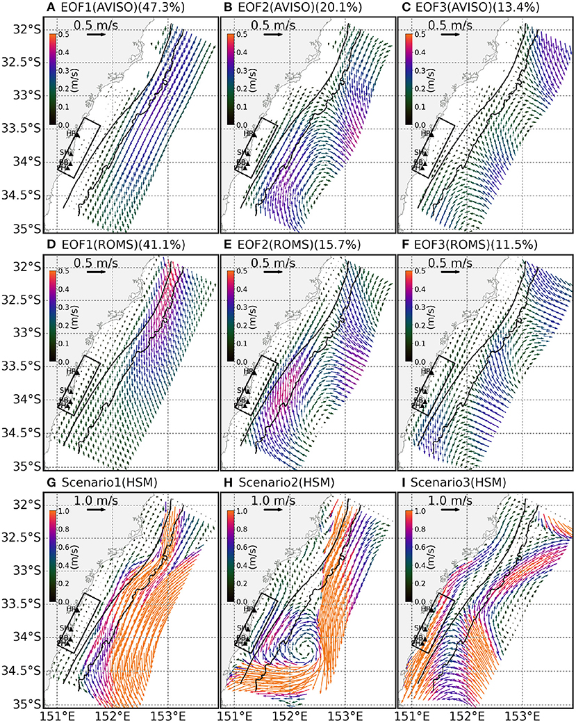
Figure 2. EOF analysis of daily velocities from the EAC-ROMS simulations and AVISO observations for the period of 1994–2019, and mean velocities of the chosen EAC scenarios from the HSM model simulations. (A–C) Spatial patterns of the three dominate EOF modes in geostrophic velocities from AVISO observations. Percentages of the explained variances for each mode are indicated. (D–F) Same as (A–C), but for surface velocities from the EAC-ROMS simulations. Panels (G–I) show the snapshots of the mean circulation patterns in the HSM model that reproduce each EAC scenario as shown in the EOF modes.

These three scenarios closely resemble the three modes identified by Ribbat et al. (2020b) in a 2-year simulation and defined by Roughan et al. (2022) to explore shelf transport pathways. However, as the modes presented here are identified from a multi-decadal (25-year) observation and simulation, we consider them to be more robust because EOF analysis can capture more time-scale variability in a longer time series.

2.3. Freshwater Inflow Scenarios

To investigate the dilution and dispersion of estuarine outflow, we add river discharges into the HSM model to represent two rainfall scenarios, provided by the Department of Planning, industry and Environment (DPIE), referred to as the “Base Case” and the “Wet event” scenarios as shown in Figure 3 and Table 1. The base case scenario represents the “base flow” and is the annual mean discharge across the estuary entrance as derived from respective calibrated models from Sydney Water Corporation. These were further verified using the observed tidal prism. The wet case scenario is an idealization representation of the “1 in 100 year” extreme flood starting on 18^th March 2021 rainstorm event. This representation is superimposed on top of the base case to give the wet event.

FIGURE 3

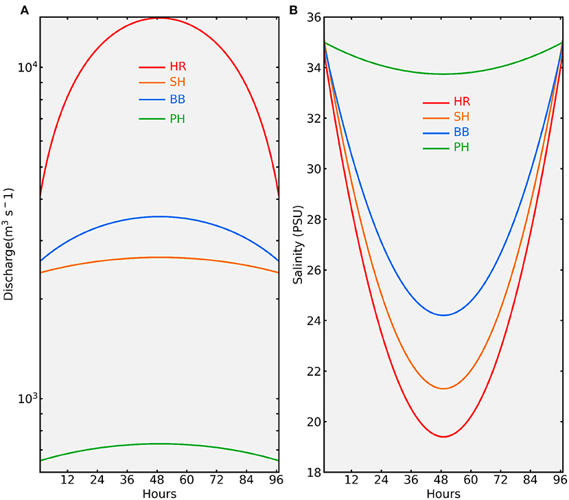
Figure 3. River discharges and salinity at the river mouths during the wet event scenarios. (A) Time series of river discharges during the wet event, the discharges return to the same constant value as base case 96 h later. Discharges of HR, SH, BB, and PH rivers are indicated with red, orange, blue, green, and black lines, respectively. (B) Same as (A), but for the salinity.

TABLE 1

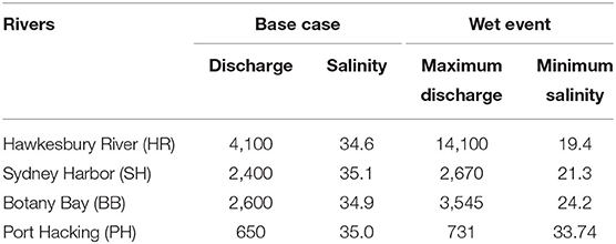
Table 1. The river discharges (m³ s⁻¹) and salinity (psu) applied at each of the four river mouths during the two rainfall scenarios “Base case” and “Wet event.”

The estuarine outflow salinity is the mean salinity observed at the DPIE Beachwatch sites near their respective estuary entrances. The four estuaries of interest are the Hawkesbury River (HR), Sydney Harbor (SH), Botany Bay (BB), and Port Hacking (PH). In the base case scenario, the river transports are constant at four river mouths, with values of 4,100 m³ s⁻¹ (HR), 2,400 m³ s⁻¹ (SH), 2,600 m³ s⁻¹ (BB), and 650 m³ s⁻¹ (PH). We also use constant surface salinity at the river mouths, with values of 34.6 (HR), 35.1 (SH), 34.9 (BB), and 35.0 (PH). In the wet events, the river transports increase rapidly and peak after 48 h, with values of 14,100 m³ s⁻¹ (HR), 2,670 m³ s⁻¹ (SH), 3,545 m³ s⁻¹ (BB), and 731 m³ s⁻¹ (PH) (Figure 3A). The surface salinity at the river mouths also decreases rapidly to 19.4 (HR), 21.3 (SH), 24.2 (BB), and 33.7 (PH) (Figure 3B). Four days later, both the river transports and salinity return to normal, with the same constant transport and salinity as the base case.

The volume flux discharges in Table 1 are the sum of the modeled mean estuarine outflows (provided by Sydney Water Corporation) and the mean freshwater catchment flow observations from the WaterNSW online database (https://realtimedata.waternsw.com.au). Estuaries such as Sydney Harbor, Botany Bay, and Port Hacking did not have a complete monitoring network, so a multiplicative factor of 2 is applied to the WaterNSW observations. This factor is estimated based on the percentage of creeks/rivers not monitored. The Hawkesbury River flow was derived from the Manly Hydraulics Laboratory (MHL) velocity observations and was not modified. The 4 day peak flow duration for the wet event is estimated from the peak flow duration for the monitored creeks.

2.4. Sensitivity Experiments

To investigate the river outflows during three dominant EAC scenarios, we choose snapshots based on the principal component of each EAC mode that represent the oceanographic circulation pattern identified by the EOF modes. As shown in Figures 2G–I, these snapshots show the mean surface velocities within the first 4 days in the HSM model simulation during the base case rainfall scenarios and represent Modes 1–3, respectively. It is clear that the chosen snapshots well represent the “EAC mode”, “EAC eddy mode”, and “EAC eddy dipole mode”, providing us the confidence to use them to simulate the impact of the EAC scenarios on the temporal and spatial evolution of the river plumes. In this study, we perform two sensitivity experiments in each EAC scenario, as described below.

To examine the different evolution of estuarine outflow between the base case and wet event, we add the dye tracers in the HSM model simulation with transports and salinity in the base case and wet event scenarios. The initial dye concentration is set to 1 kg m⁻³. The temperature profiles at the river mouths are extracted from the monthly climatology of the EAC-ROMS multi-decadal simulations. We also use climatological salinity in the bottom 20 layers at the river mouths, but the salinity linearly increases with depth in the top 10 layers. The river discharge decreases with depth at the river mouths, with 55% of the outflow are in the top 10 layers.

In each EAC scenario, the initial and boundary conditions for the HSM model are taken from the parent EAC-ROMS model during the time period identified in each of the representative scenarios. To get a more realistic simulation, we spin up the HSM model with base case river outflows and salinity for 7 days before adding the dye tracer. This short period of spin up allows the low salinity water to mix with shelf water and spread out of the river mouth. After the initial spin up, we perform two model runs of 15 days duration with river transports and salinity representing the two rainfall scenarios. The simulations in the first 4 days are used for comparison.

3. Results

3.1. Spatial Distributions of River Plume

To compare the difference of river plumes between the base case and wet event, we averaged the surface dye concentration over the first 4 days in the Hawkesbury Shelf bioregion (Figure 4). The mean dye concentration around the river mouth is much larger in the wet event than in the base case, particularly in the Hawkesbury River region (Figures 4G–I). In this study, we focus on the evolution of the river plume around the Hawkesbury River because it has the largest discharge among four rivers (Figure 3A), which is more than four times larger than the other rivers. In the base case, the river plume dispersal varies in different EAC scenarios (Figures 4A–C). In EAC scenario 1 (Figure 4A), the river plume spreads both northward and southeastward near the coast. However, in EAC scenario 2 (Figure 4B), the river plume dispersal is toward the north due to the impact of the cyclonic eddies on the shelf. In EAC scenario 3 (Figure 4C), most of the river plume spreads southward, with some to the north. In the wet event, the evolution of river plumes shows the same spatial patterns as that in the base case (Figures 4D–F), but with a much larger area due to the increase in river discharges. The river plume spreads further southeast in EAC scenario 1, but more onshore in EAC scenario 3. The largest differences appear east, south and north of the river mouth in EAC scenario 1 and EAC scenario 3 (Figures 4G,I), but east and north of the river mouth in EAC scenario 2 (Figure 4H).

FIGURE 4

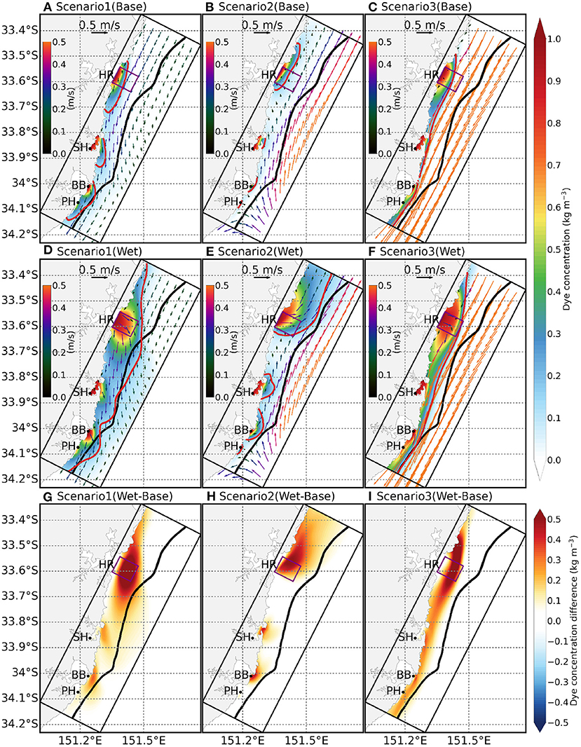
Figure 4. Spatial distributions of dye concentration averaged over the first 4 days for each EAC scenario and their differences between the wet event and the base case. (A–C) Spatial distributions of dye concentration for EAC scenario 1, EAC scenario 2, and EAC scenario 3 in the base case. The solid black line shows the 100 m isobath, and the red line indicates the contour of 0.15 dye concentration. The vectors show the mean surface velocities. (D–F) Same as (A–C), but for the wet event. (G–I) Differences of dye concentration for three EAC scenarios between the wet event (D–F) and the base case (A–C).

The evolution of the river plume also relies on the initial salinity at the river mouths because the salinity contributes to the density structure, which affects the background currents. Compared to the spatial distributions of dye concentration, the low sea surface salinity (SSS) has consistent patterns in all EAC scenarios of both the base case and wet event (Figure 5). This suggests that the SSS we used here at the river mouth can well represent the evolution of the river plume, which can be captured in both the low salinity freshwater and dye concentration. This gives us confidence that the sensitivity experiments in this study can be used to understand the dilution of estuarine outflow during large rainfall events.

FIGURE 5

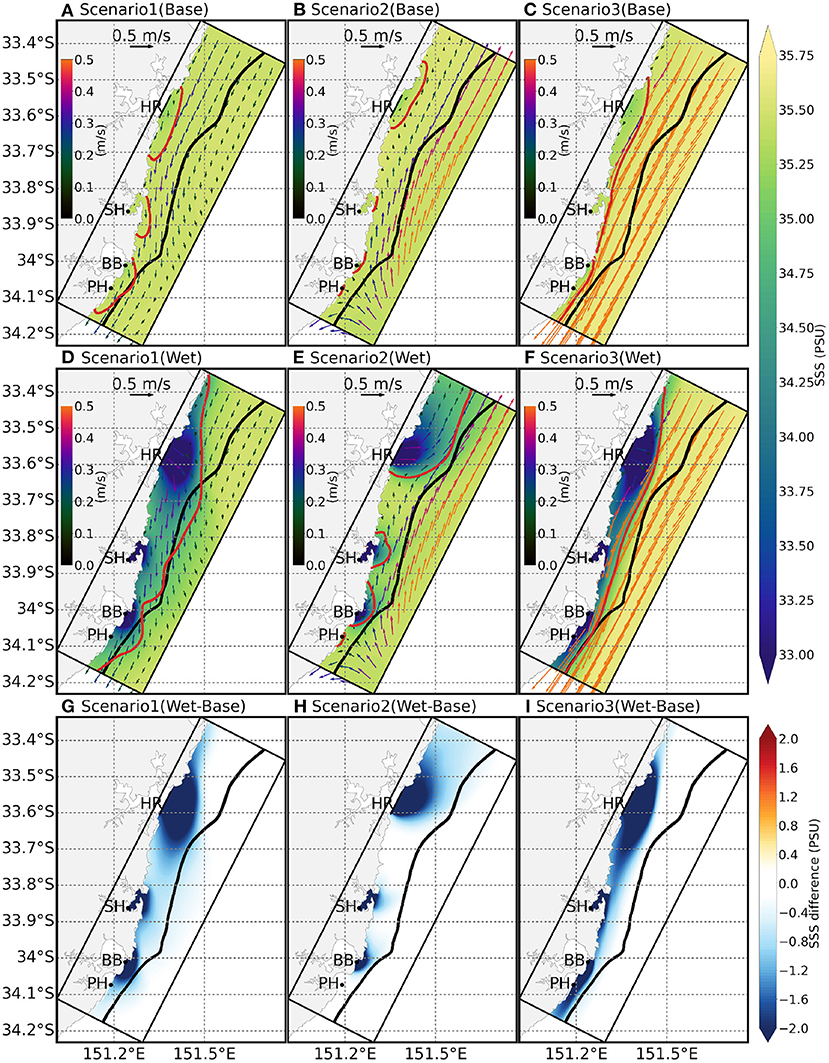
Figure 5. Spatial distributions of SSS averaged over the first 4 days for each EAC scenario and their differences between the wet event and the base case. (A–C) spatial distributions of SSS for EAC scenario 1, EAC scenario 2, and EAC scenario 3 in the base case. The solid black line shows the 100 m isobath, and the red line indicates the contour of 0.15 dye concentration. The vectors show the mean surface velocities. (D–F) Same as (A–C), but for the wet event. (G–I) Differences of SSS for three EAC scenarios between the wet event (D–F) and the base case (A–C).

Due to the large outflow at the Hawkesbury River, this region has the largest dye concentration and lowest salinity. As the dye concentration was 1 for the freshwater and 0 for the pure sea water, to identify the vertical penetration of the river plume, we estimate the freshwater thickness induced by the rivers as $T_{\text{freshwater}}={\displaystyle {\int }_{\eta }^{-H}cdz}$. H is the water depth, η is the sea surface height, and c is the dye concentration. As shown in Figure 6, freshwater thickness is larger than 10 m within the dye concentration of 0.15 around the river mouth in the base case. We also found the freshwater thickness of ~3 m south of the river mouth in EAC scenario 1 and EAC scenario 3 (Figures 6A,C) and north of the river mouth in EAC scenario 2 (Figure 6B). In the wet event, large discharges increase the area of freshwater thickness as indicated by the dye concentration of 0.15 in Figures 6D–F. In EAC scenario 1 and EAC scenario 3, large freshwater thickness difference between the base case and wet event can be found east, south and north of the river mouth (Figures 6G–I). In EAC scenario 2, the freshwater thickness difference is much smaller and appears north of the river mouth (Figure 6H).

FIGURE 6

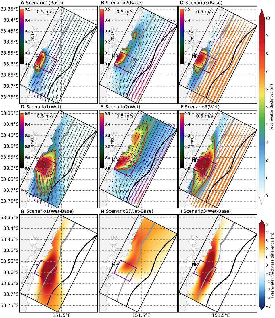
Figure 6. Spatial distributions of freshwater thickness averaged over the first 4 days for each EAC scenario in the HR region and their differences between the wet event and the base case. (A–C) spatial distributions of freshwater thickness for EAC scenario 1, EAC scenario 2, and EAC scenario 3 in the base case. The solid gray and black lines show the 50 and 100 m isobath, respectively. The red line indicates the freshwater thickness contour of 4 m, and the purple box shows the location used in the following Figures 7, 8, 10. The vectors show the mean surface velocities. (D–F) Same as (A–C), but for the wet event. (G–I) Differences of freshwater thickness for three EAC scenarios between the wet event (D–F) and the base case (A–C).

3.2. Cross-Section of the Plume at Hawkesbury River

As discussed in section 3.1, the largest difference of dye concentration, SSS and freshwater thickness between the base case and wet event can be found in the purple box in Figure 6. To investigate the vertical evolution and eastward dispersal of the river plume, we calculate the averaged dye concentration, salinity, along-shore and cross-shore velocities within the purple box.

Figure 7 shows the cross-section of dye concentration east of the river mouth. As indicated by the red line, the maximum eastward extension can reach around 4 km in EAC scenario 2 (Figure 7B), with a high dye concentration (0.5) about 2 km away from the river mouth. The river plume spreads much farther in EAC scenario 1 and EAC scenario 3 (Figures 7A,C). The vertical impact reaches about 20 m in EAC scenario 2, but is only 15 m and 13 m in EAC scenario 1 and EAC scenario 3, respectively.

FIGURE 7

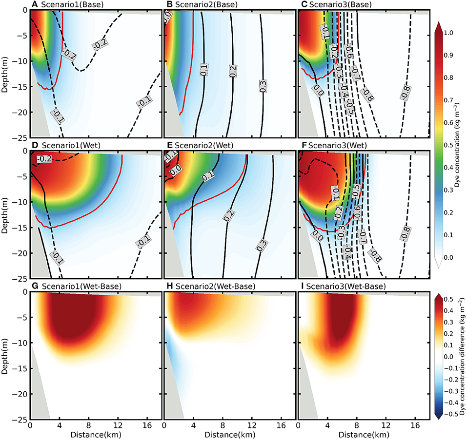
Figure 7. Cross-section profiles of dye concentration averaged over the first 4 days within the purple box in Figure 6 for each EAC scenario and their differences between the wet event and the base case. (A–C) Cross-sections profiles of dye concentration for EAC scenario 1, EAC scenario 2, and EAC scenario 3 in the base case. The solid and dashed black lines show the northward and southward velocities, respectively. The red line indicates the contour of 0.15 dye concentration. (D–F) Same as (A–C), but for the wet event. (G–I) Differences of dye concentration for three EAC scenarios between the wet event (D–F) and the base case (A–C). Only the dye concentration profiles less than 18 km from the river mouth are shown.

In the wet event, the eastward velocities increase significantly at the river mouth in three EAC scenarios. the maximum eastward extension is about 12.5, 11.5, and 9.5 km in EAC scenario 1, EAC scenario 2 and EAC scenario 3, respectively (Figures 7D–F). High dye concentration also spreads farthest in EAC scenario 1, but nearest in EAC scenario 2. The vertical penetration of high dye concentration is the deepest in EAC scenario 3 but the shallowest in EAC scenario 2. The differences of dye concentration between the wet event and base case are constrained within 2–12 km away from the river mouth and 12 m depth in EAC scenario 1 (Figure 7G). Compared to EAC scenario 1, the difference is much smaller in EAC scenario 2 (Figure 7H). In EAC scenario 3, the difference appears within 2–9 km away from the river mouth but reach about 15 m depth (Figure 7I).

The vertical profiles of salinity show similar patterns to dye concentration (Figure 8). The salinity differences of salinity near the river mouth and offshore water are very small in the base case (Figures 8A–C). However, in the wet event, the salinity decreases significantly due to the increase in river discharges (Figures 8D–F). The difference of salinity between wet event and base case starts from the river mouth to 8–21 km (Figures 8G–I).

FIGURE 8

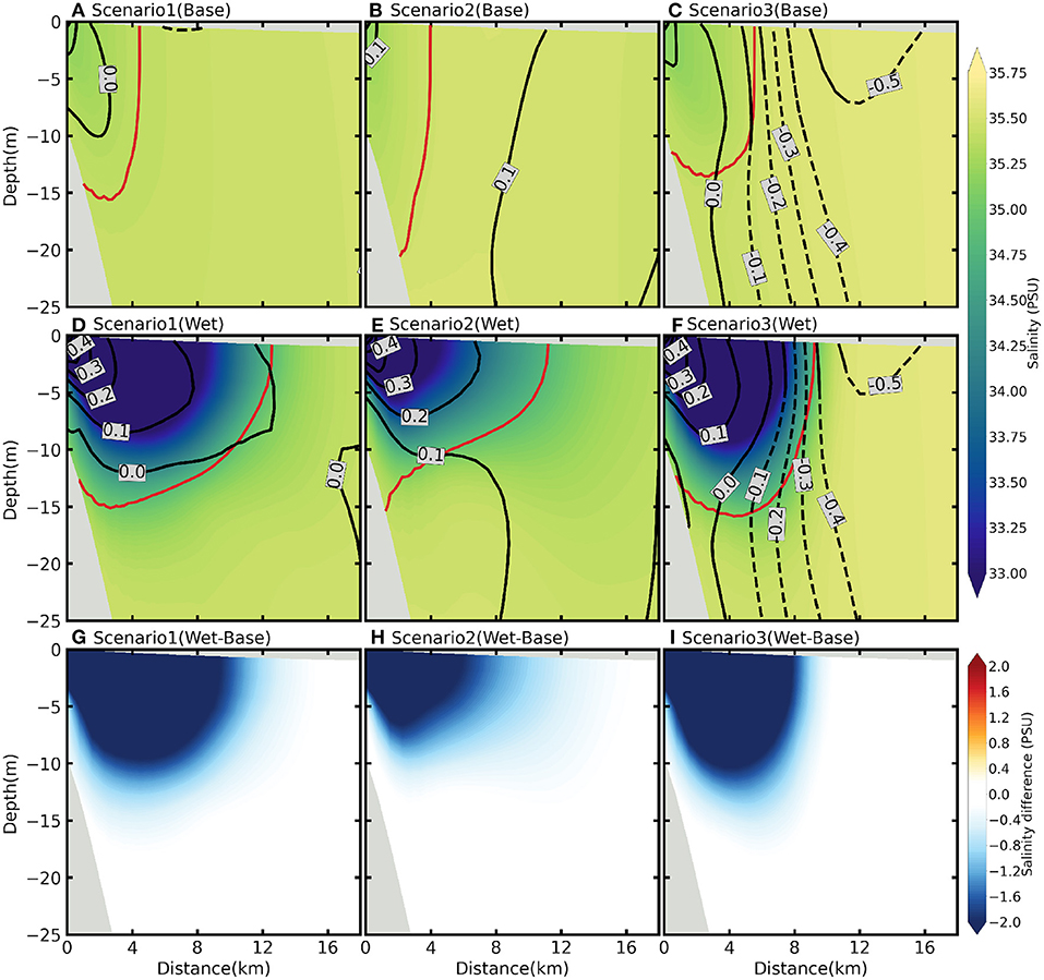
Figure 8. Cross-section profiles of salinity averaged over the first 4 days within the purple box in Figure 6 for each EAC scenario and their differences between the wet event and the base case. (A–C) Cross-section profile of salinity for EAC scenario 1, EAC scenario 2, and EAC scenario 3 in the base case. The solid and dashed black lines show the eastward and westward velocities, respectively. The red line indicates the contour of 0.15 dye concentration. (D–F) Same as (A–C), but for the wet event. (G–I) Differences of salinity for three EAC scenarios between the wet event (D–F) and the base case (A–C). Only the salinity profiles less than 18 km from the river mouth are shown.

3.3. Temporal Evolution of River Plume

To investigate the horizontal dispersion of the river plume, we estimate the freshwater area as

$\begin{array}{ll}{A}_{\text{freshwater}}=\int cdxdy.& (1)\end{array}$

Following the method in Duran-Matute et al. (2014) and Yu et al. (2020), we can also calculate the amount of freshwater volume and the transport through a transect as follows:

$\begin{array}{llll}{V}_{\text{freshwater}}& =& \int cdxdydz& (2)\end{array}$

$\begin{array}{llll}{Q}_{\text{freshwater}}& =& {\displaystyle \underset{A}{\int }}c*u_{n}dA& (3)\end{array}$

where u_n is the velocity component normal to the transect.

Figure 9A shows the temporal evolution of the river plume around the Hawkesbury River. The difference in the freshwater area between the wet event and base case increase with time in the first 2 days due to increased river discharges, with the largest difference in the EAC scenario 1. It takes around 6 days for the freshwater area in the wet event to return to the same level as the base case. The freshwater areas in the wet event averaged within the first 4 days are much larger than those in the base case (Figure 9C). The EAC scenario 1 in the wet event has the largest freshwater area of 6.10 × 10⁸ m². The smallest freshwater area can be found in the EAC scenario 2 in the base case, which is 1.99 × 10⁸ m². The freshwater volume shows consistent temporal variation with the freshwater area (Figures 9A,B), that the EAC scenario 1 has the largest difference. Within the first 4 days, the freshwater volumes in the wet event are larger than those in the base case for three EAC scenarios (Figures 9B,D).

FIGURE 9

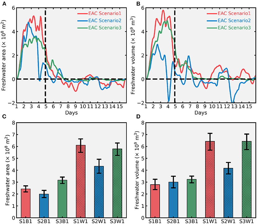
Figure 9. Time series of freshwater area and volume difference between the base case and wet event for each EAC scenario during the whole simulation period. (A) Time series of freshwater area. The solid (dashed) red, blue, and green lines indicate EAC scenario 1, EAC scenario 2, and EAC scenario 3 in the base case (wet event), respectively. (B) Same as (A), but for the freshwater volume. (C) Freshwater area averaged within the first 4 days for the base case (unhatched bars) and wet event (hatched bars). The red, blue, and green bars indicate EAC scenario 1, EAC scenario 2, EAC scenario 3, respectively. (D) Same as (C), but for the freshwater volume.

To examine the along-shore and cross-shore extension of the river plumes at the Hawkesbury River, we calculate the freshwater transport across the east, north and south faces of the purple box in Figure 10. Large river discharges at the river mouth increase the eastward velocities, which facilitate the eastward extension of the river plume. As shown in Figure 10A, the eastward extension of the river plume varies with the discharge, with large transport within the first 4 days. The eastward transports in EAC scenario 1 and EAC scenario 2 indicate that the river plume flows out of the box from the east face (Figure 10D). However, the transport is westward in EAC scenario 3 across the east face, implying that the background current impedes the river plume extends further east. The along-shore transports are more variable (Figures 10B,C), the freshwater flows into and out of the box from both the north and south faces. Time series of northward and southward transports also show the along-shore extension are much farther in the wet event when river discharges are larger. Within the first 4 days, the along-shore extension is mainly northward in EAC scenario 2 due to the existence of the cyclonic eddies (Figure 10E), and it is poleward in EAC scenario 1 and EAC scenario 3 because of the EAC jet and the eddy dipoles (Figure 10F).

FIGURE 10

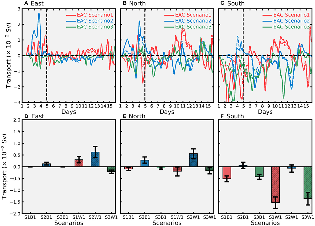
Figure 10. Time series of freshwater transport to the north, south and east for each EAC scenario in the base case and wet event during the whole simulation period. (A) Time series of freshwater transport along the east side of the purple box in Figures 4, 6. The solid (dashed) red, blue, and green lines indicate EAC scenario 1, EAC scenario 2, EAC scenario 3 in the wet event (base case), respectively. (B,C) Same as (A), but for the north and south side of the box. (D) Freshwater transport averaged within the first 4 days for the base case (unhatched bars) and wet event (hatched bars). (E,F) Same as (D), but for the north and south side of the box.

4. Discussion

4.1. Role of Mesoscale Circulation on River Plumes

In the Hawkesbury Shelf marine bioregion, the circulation is influenced by the onshore encroachment of the EAC (Roughan and Middleton, 2004; Archer et al., 2017; Malan et al., 2020; Xie et al., 2020, 2021) and the western branch of both mesoscale anticyclonic and cyclonic eddies (Oke and Griffin, 2011; Schaeffer et al., 2013). As the EAC jet and the anticyclonic eddies encroach upon the coast, their shoreward movements accelerate the poleward along-shore current. However, the intrusion of cyclonic eddies result in a northward flow on the shelf (Kerry et al., 2020; Ribbat et al., 2020b; Roughan et al., 2022). Therefore, the variability of the EAC jet and the eddy field play a role in the evolution of the river plumes near the coast. Here we show different spatial patterns of the main river plumes in the Hawkesbury Shelf bioregion influenced by the 3 dominant mesoscale circulation modes, the “EAC mode”, “EAC eddy mode”, and “EAC eddy dipole mode”. Our results indicate that the spatial structure and dispersion of the river plumes are associated with the mesoscale circulation.

Malan et al. (2020) examined individual eddy dipole events from satellite altimetry observations and found that the cyclonic eddy often co-occurs during the shedding of the anticyclonic eddy from the EAC jet, which sets up a large horizontal shear field between the north branch of the eddy and the EAC flowing offshore to the east. Li et al. (2021b, 2022) showed that both the upstream EAC volume transport and westward propagation of Rossby waves modulate the latitude of the EAC separation and further control the formation and position of mesoscale eddies and eddy dipoles. Here we showed the links between the mesoscale ocean dynamics and the regional river plume extensions, and the dynamics and underlying controlling mechanisms of these mesoscale features will be the topic of future work.

Our results show that the low salinity fresh water from the river mouth extends northward and southeastward in EAC scenario 1, disperses northward and eastward in EAC scenario 2, and spreads southward with some to the north in EAC scenario 3. Each scenario is dictated by the position of the EAC jet in relation to the cyclonic and anticyclonic eddy. In EAC scenario 1, the EAC jet dominates the flow, driving the plume poleward and offshore in the southern part of the domain. In EAC scenario 2, the cyclonic eddy is located directly adjacent to the Hawkesbury Shelf region, driving a northward flow, and some shelf export to the north. Offshore transport (Figure 7) is the largest in EAC scenario 1 and 2. In EAC scenario 3, the plume is dictated by the location of the anticyclonic eddy, which traps the plume by the coast.

In the South Brazilian Bight and South Brazil, a permanent continuous Brazil Current flows southward along the slope. By releasing passive dyes together with the river discharge in the hydrodynamical model, Marta-Almeida et al. (2021) showed that the local river plumes are confined to the inner shelf because the strong and persistent large-scale Brazil Current flowing southward over the slope prevents the river plumes from interaction with offshore oceanic mesoscale dynamics. The effect of mesoscale eddies on river plumes was conducted in the Agulhas Mozambique Channel region (Malauene et al., 2018), where the circulation is dominated by trains of intermittent, passing mesoscale eddies. They showed that offshore passing eddies modulate river plumes direction and spread depends on their strength and proximity to the shelf. The Zambezi River plume is bi-directional, which is associated with mesoscale eddies. The southward-directed plume was clearly detached from the coast and directly related to offshore anticyclonic eddies which were able to induce a southward current over most of the shelf. They suggested that offshore mesoscale eddies should be taken into account when studying the river plumes of the Sofala Bank. The Hawkesbury Shelf region is located downstream of the EAC separation, where the shelf circulation is dominated by three prominent EAC modes. Here we showed that both the large-scale EAC and mesoscale eddies play roles in modulating the river plumes.

Interestingly, a study of the interaction of loop current eddies with the Mississippi River plume also showed that eddy pairs (what we term an eddy dipole) controlled offshore export pathways of riverine material (Schiller et al., 2011). As in the EAC system, eddy dipoles can generate coherent cross-shelf flows. These results demonstrate that the configuration of eddy dipoles and proximity of eddies to the shelf break strongly determines the characteristics of offshore freshwater transport. The three EAC scenarios and the position of the cyclonic eddy dictate the variability in the along-shore and offshore pathways that the plume may take.

Our study supports the findings of Schiller et al. (2011), who show that in order to obtain a complete picture of the dynamics impacting river plume dispersal, mesoscale circulation must be considered. In this case, it is necessary to downscale larger domain coarser models that resolve the mesoscale circulation properly in higher resolution nested models that better resolve shelf circulation. Nesting within a data assimilating model (e.g., Kerry et al., 2020) will ensure realistic connections between the shelf and the deep ocean if specific case studies are to be explored as per (Roughan et al., 2022).

4.2. Impact of River Discharge on the Shelf Circulation

On the one hand, the mesoscale circulation can influence the spatial and temporal evolution of river plumes. On the other hand, the river discharge also affects the stratification, instabilities, shelf circulation and dynamics at the submesoscale over the shelf, which is relevant to the ecosystem and biogeochemical processes. Large river plume plays a significant role in regulating the shelf circulation, which intensifies the cross-shelf exchange (Wu et al., 2021). River outflow can also enhance the submesoscale currents by increasing lateral buoyancy gradients but suppresses them by decreasing the boundary layer depth (Barkan et al., 2017). As this study focuses on the response of river plumes to the mesoscale circulation, all the above critical processes are neglected. In future work, we aim to focus on the effects of the river discharge on the shelf circulation and dynamics, and we will take advantage of the high-resolution model to understand the critical duration and river discharge of transport that is required to affect the shelf dynamics at submesoscale.

4.3. Secondary Drivers of Plume Structure

Downstream of the EAC separation point, coastal wind stress is the secondary driver of shelf circulation through Ekman transport mechanisms (Schaeffer et al., 2013). In this region, (Rossi et al., 2014) showed that prolonged downwelling favorable winds (for greater than 5 days) occur up to 31% of the year, where as upwelling winds (for greater than 5 days) only occur for 4% of the year. Downwelling favorable winds (from the south) act to mix the water column and result in northward flow close to the coast. Periods of heavy rainfall are often associated with winds from the south, which could act to drive the plumes to the north. An upwelling favorable wind (from the north) combined with EAC encroachment leads to the strongest poleward along-shore velocities on the shelf and offshore cross-shelf surface transport, but the downwelling favorable winds play an opposite role (Schaeffer et al., 2013; Archer et al., 2017). The impact of coastal winds on the dispersion of river plumes in each EAC scenario deserves further exploration, particularly the coupled effect of strong winds that drive storms, heavy rainfall and waves.

In addition to mesoscale circulation and local wind forcing, tides can also impact the river plume structure. In large river plumes, tidal currents act to stabilize the offshore growth of river-plume bulges in the coastal and shelf region (Isobe, 2005; Li and Rong, 2012) or enhance the downstream along-shore freshwater transport by compressing the bulge shoreward against the coast (Chen, 2014). At the northern side of the Changjiang River mouth, the tidal forcing can increase the vertical mixing, resulting in the formation of a strong along-coast salinity gradient that restricts the northward extension of the plume (Wu et al., 2011). At the Berau River mouth, tides cause vertical mixing and suppress the cross-shelf spreading of the river plume (Tarya et al., 2015). Although tidal forcing was included in our simulation, as both the river outflow and tidal circulation are “weak” in our region we expect the effect of tidal forcing to be small. Future studies could improve our understanding of the impact of tides on river plumes adjacent to the EAC.

4.4. Multi-Scale Variability of the River Plumes

The EAC flow and its associated eddy field vary on seasonal and interannual timescales, which may also impact river plume evolution. Previous studies have demonstrated the seasonality of the EAC flow, where it is stronger in Austral summer (Dec-Feb) than in Austral winter (Jun-Aug) (Ridgway, 1997; Archer et al., 2017; Kerry and Roughan, 2020). As discussed in Li et al. (2021b), there is strong interannual variability of eddy activity around the typical EAC separation region, which is related to the EAC transport upstream. As such, the frequency and magnitude of the chosen EAC scenarios in the present study (that well represent the three dominant EAC modes) may vary across seasons and longer timescales.

4.5. Sensitivity to Freshwater Inflow

Historic observations of plume extents by Kingsford and Suthers (1994) showed that Botany Bay plumes could range in offshore extension from 2 km during a dry spell to 11 km during large rainfall events. They also noted that the plumes were shallow ranging 2–8 m deep above higher density coastal waters. These values agree well with the plume dimensions presented here (9.5–12 km in horizontal, 13–20 m in vertical). Hence our sensitivity studies with idealized river discharges provide the best estimate on the middle and upper limit of the river plume dispersal over the Hawkesbury Shelf under the three circulation scenarios. This means the results can be used to explore a range of ecological impacts of the river plumes and their offshore extents.

4.6. Ecological Implications

The contrasting river plume structures presented in the three EAC scenarios will have differing impacts on the local hydrodynamics, water environment and ecological processes. Firstly, river plumes can drive the distribution and dispersion of material (e.g., sediment, marine litter, or metals) coming out of the estuaries (Jaffe et al., 1995; Warrick et al., 2004). We also know that eddies impact the transport and distribution of larval fish (Roughan et al., 2011) and crustacea in the region (Cetina-Heredia et al., 2019).

Large rainfall events can maintain and enhance biological productivity due to lower salinity water altering habitat availability. Locally, Kingsford and Suthers (1994) found major differences in larval fish and zooplankton distributions and abundance in the Botany Bay plume. It has been shown that fresh water can affect the distribution of commercially fished prawns (Gammelsrød, 1992), and it is thought that river plumes may impact fish activity (Gillson, 2011; Gillson et al., 2012). This implies that the flood events may produce different fish distribution and abundance in the three dominant EAC scenarios, thereby having a commercial fisheries impact. Hence each of these mesoscale circulations combined with the river plume scenarios may also affect the population dynamics of marine organisms.

Here we showed that the river plume has the largest freshwater area and eastward extension (12.5 km) during the large rainfall event in the “EAC mode”. The salinity around the river mouth decreases rapidly in this EAC scenario, which likely creates a physical barrier to the recruitment of marine taxa and reduces available nursery habitat both north, southeast and east of the river mouth. In the “EAC eddy mode”, the impact of the river plumes on the local ecological system mainly covers the north and east of the river mouth because the freshwater driven by the proximity of the cyclonic eddy carries large quantities of suspended sediment toward these directions. In the “EAC dipole mode”, the river plume mainly spreads southward driven by the western branch of the anticyclonic eddy, decreasing the salinity south of the river mouth.

5. Conclusion

Using a high-resolution (750 m) hydrodynamic model, we simulate four idealized river plumes in the Hawkesbury bioregion during three dominant mesoscale circulation scenarios and investigate the spatial and temporal evolution of river plumes in the base case and wet event. We compare the spatial patterns of river plumes during each EAC scenario and explore the impact of the mesoscale circulation on the plume dispersion. We focus on the Hawkesbury River plume as it has the largest discharge among the four rivers examined. We find the river plumes have significantly different 3 dimensional structures in response to the mesoscale circulation scenarios. In all scenarios, the plume remains trapped by the coast with an offshore extent of less than 12 km. In the “EAC mode”, the plume spreads both northward and southeastward. The offshore spread in this scenario is the largest, which is around 12.5 km to the east of the river mouth in the wet event. In the “EAC eddy mode”, this plume dispersal is toward the north and east, driven by the proximity of a cyclonic eddy on the shelf, with an eastward extension of 11.5 km. In the “EAC eddy dipole mode”, most of this river plume spreads southward with some to the north, again dictated by the position of the cyclonic eddy. The cross-shelf dispersal is a minimum of 9.5 km from the river mouth. The difference of the freshwater spatial extent of the plume between the wet event and base case is the largest in EAC scenario 1 and the smallest in EAC scenario 2. Our results have far-reaching implications for the understanding of ecological systems and provide guidance for the local and state government bodies. Knowledge regarding the ultimate fate of riverborne material, dilution and cumulative effects (e.g., over long times and from multiple sources) will enable better environmental management of this dynamic region.

Data Availability Statement

EAC-ROMS model initial and boundary conditions are provided by CSIRO Australia BRAN2020 and available at https://research.csiro.au/bluelink/outputs/data-access/. The atmospheric forcing BARRA-R data are obtained from http://www.bom.gov.au/research/projects/reanalysis/. The tide forcing is obtained from https://www.tpxo.net/global/tpxo8-atlas. The AVISO products are downloaded from https://resources.marine.copernicus.eu/product-detail/SEALEVEL_GLO_PHY_L4_MY_008_047/INFORMATION. The EAC-ROMS model output (https://doi.org/10.26190/TT1Q-NP46) is available at https://researchdata.edu.au/high-resolution-22-version-20/1676421 and should be cited as (Li et al., 2021a).

Author Contributions

MR, SR, and JL conceived the study and developed the conceptual framework. CK configured and validated the EAC-ROMS model. JL ran the EAC-ROMS and HSM model and analyzed the model results. All authors contributed to interpreting the results and writing and editing the manuscript. All authors contributed to the article and approved the submitted version.

Funding

This research was partially supported by the New South Wales Department of Planning, Industry and Environment. Former model development was partially supported by the Australian Research Council grants LP120100592, DP140102337, LP160100162, and LP170100498. This research was undertaken with the assistance of resources and services from the National Computational Infrastructure (NCI), which is supported by the Australian Government. This research also includes computations using the computational cluster Katana https://doi.org/10.26190/669X-A286, supported by Research Technology Services at UNSW Sydney.

Conflict of Interest

The authors declare that the research was conducted in the absence of any commercial or financial relationships that could be construed as a potential conflict of interest.

Publisher's Note

All claims expressed in this article are solely those of the authors and do not necessarily represent those of their affiliated organizations, or those of the publisher, the editors and the reviewers. Any product that may be evaluated in this article, or claim that may be made by its manufacturer, is not guaranteed or endorsed by the publisher.

References

Archer, M. R., Roughan, M., Keating, S. R., and Schaeffer, A. (2017). On the variability of the east Australian current: jet structure, meandering, and influence on shelf circulation. J. Geophys. Res. Oceans 122, 8464–8481. doi: 10.1002/2017JC013097

CrossRef Full Text | Google Scholar

Barkan, R., McWilliams, J. C., Shchepetkin, A. F., Molemaker, M. J., Renault, L., Bracco, A., et al. (2017). Submesoscale dynamics in the northern Gulf of Mexico. Part I: Regional and seasonal characterization and the role of river outflow. J. Phys. Oceanogr. 47, 2325–2346. doi: 10.1175/JPO-D-17-0035.1

CrossRef Full Text | Google Scholar

Cetina-Heredia, P., Roughan, M., Liggins, G., Coleman, M. A., and Jeffs, A. (2019). Mesoscale circulation determines broad spatio-temporal settlement patterns of lobster. PLoS ONE 14, e0211722. doi: 10.1371/journal.pone.0211722

PubMed Abstract | CrossRef Full Text | Google Scholar

Cetina-Heredia, P., Roughan, M., Sebille, E. V., and Coleman, M. A. (2014). Long-term trends in the East Australian Current separation latitude and eddy driven transport. J. Geophys. Res. Oceans 119, 4351–4366. doi: 10.1002/2014JC010071

CrossRef Full Text | Google Scholar

Chamberlain, M. A., Oke, P. R., Fiedler, R. A. S., Beggs, H. M., Brassington, G. B., and Divakaran, P. (2021). Next generation of bluelink ocean reanalysis with multiscale data assimilation: Bran2020. Earth Syst. Sci. Data 13, 5663–5688. doi: 10.5194/essd-13-5663-2021

CrossRef Full Text | Google Scholar

Chen, S. N. (2014). Enhancement of alongshore freshwater transport in surface-advected river plumes by tides. J. Phys. Oceanogr. 44, 2951–2971. doi: 10.1175/JPO-D-14-0008.1

CrossRef Full Text | Google Scholar

Colberg, F., Brassington, G. B., Sandery, P., Sakov, P., and Aijaz, S. (2020). High and medium resolution ocean models for the Great Barrier Reef. Ocean Modell. 145:101507. doi: 10.1016/j.ocemod.2019.101507

CrossRef Full Text | Google Scholar

Covelli, S., Piani, R., Acquavita, A., Predonzani, S., and Faganeli, J. (2007). Transport and dispersion of particulate Hg associated with a river plume in coastal Northern Adriatic environments. Mar. Pollut. Bull. 55, 10–12. doi: 10.1016/j.marpolbul.2007.09.006

PubMed Abstract | CrossRef Full Text | Google Scholar

Dawson, K. (2002). Fish kill events and habitat losses of the Richmond River, NSW Australia: an overview. J. Coast. Res. 36, 216–221. doi: 10.2112/1551-5036-36.sp1.216

CrossRef Full Text | Google Scholar

Ducet, N., Le Traon, P. Y., and Reverdin, G. (2000). Global high-resolution mapping of ocean circulation from TOPEX/Poseidon and ERS-1 and -2. J. Geophys. Res. Oceans 105, 477–498. doi: 10.1029/2000JC900063

CrossRef Full Text | Google Scholar

Duran-Matute, M., Gerkema, T., De Boer, G. J., Nauw, J. J., and Gräwe, U. (2014). Residual circulation and freshwater transport in the Dutch Wadden Sea: a numerical modelling study. Ocean Sci. 10, 611–632. doi: 10.5194/os-10-611-2014

CrossRef Full Text | Google Scholar

Egbert, G. D., and Erofeeva, S. Y. (2002). Efficient inverse modeling of barotropic ocean tides. J. Atmos. Ocean. Technol. 19, 183–204. doi: 10.1175/1520-0426(2002)019<0183:EIMOBO>2.0.CO;2

CrossRef Full Text | Google Scholar

Eyre, B. D., Kerr, G., and Sullivan, L. A. (2006). Deoxygenation potential of the Richmond river estuary floodplain, northern NSW, Australia. River Res. Appl. 22, 981–992. doi: 10.1002/rra.950

CrossRef Full Text | Google Scholar

Gammelsrød, T. (1992). Variation in shrimp abundance on the Sofala Bank, Mozambique, and its relation to the Zambezi River runoff. Estuar. Coast. Shelf Sci. 35, 91–103. doi: 10.1016/S0272-7714(05)80058-7

CrossRef Full Text | Google Scholar

Gillson, J. (2011). Freshwater flow and fisheries production in estuarine and coastal systems: where a drop of rain is not lost. Rev. Fish. Sci. 19, 168–186. doi: 10.1080/10641262.2011.560690

CrossRef Full Text | Google Scholar

Gillson, J., Suthers, I., and Scandol, J. (2012). Effects of flood and drought events on multi-species, multi-method estuarine and coastal fisheries in eastern Australia. Fish. Manage. Ecol. 19, 54–68. doi: 10.1111/j.1365-2400.2011.00816.x

CrossRef Full Text | Google Scholar

Grimes, C. B. (2001). Fishery production and the Mississippi River discharge. Fisheries 26, 17–26. doi: 10.1577/1548-8446(2001)026<0017:FPATMR>2.0.CO;2

PubMed Abstract | CrossRef Full Text | Google Scholar

Isobe, A. (2005). Ballooning of river-plume bulge and its stabilization by tidal currents. J. Phys. Oceanogr. 35, 2337–2351. doi: 10.1175/JPO2837.1

CrossRef Full Text | Google Scholar

Jaffe, R., Leal, I., Alvarado, J., Gardinali, P., and Sericano, J. (1995). Pollution effects of the Tuy River on the central Venezuelan coast: anthropogenic organic compounds and heavy metals in Tivela mactroidea. Mar. Pollut. Bull. 30, 820–825. doi: 10.1016/0025-326X(95)00087-4

CrossRef Full Text | Google Scholar

Kannan, N., Kim, M., Hong, S. H., Jin, Y., Yim, U. H., Ha, S. Y., et al. (2012). Chemical tracers, sterol biomarkers and satellite imagery in the study of a river plume ecosystem in the Yellow Sea. Continent. Shelf Res. 33, 29–36. doi: 10.1016/j.csr.2011.10.001

CrossRef Full Text | Google Scholar

Kerry, C., Powell, B., Roughan, M., and Oke, P. (2016). Development and evaluation of a high-resolution reanalysis of the East Australian Current region using the Regional Ocean Modelling System (ROMS 3.4) and Incremental Strong-Constraint 4-Dimensional Variational (IS4D-Var) data assimilation. Geosci. Model Dev. 9, 3779–3801. doi: 10.5194/gmd-9-3779-2016

CrossRef Full Text | Google Scholar

Kerry, C., and Roughan, M. (2020). Downstream evolution of the east Australian current system: mean flow, seasonal, and intra-annual variability. J. Geophys. Res. Oceans 125, e2019JC015227. doi: 10.1029/2019JC015227

CrossRef Full Text | Google Scholar

Kerry, C., Roughan, M., and Powell, B. (2020). Predicting the submesoscale circulation inshore of the East Australian current. J. Mar. Syst. 204, 103286. doi: 10.1016/j.jmarsys.2019.103286

CrossRef Full Text | Google Scholar

Kingsford, M. J., and Suthers, I. M. (1994). Dynamic estuarine plumes and fronts: importance to small fish and plankton in coastal waters of NSW, Australia. Continent. Shelf Res. 14, 655–672. doi: 10.1016/0278-4343(94)90111-2

CrossRef Full Text | Google Scholar

Kroon, F. J., and Ludwig, J. A. (2010). Response and recovery of fish and invertebrate assemblages following flooding in five tributaries of a sub-tropical river. Mar. Freshw. Res. 61, 86–96. doi: 10.1071/MF08357

CrossRef Full Text | Google Scholar

Lawrence, M. G. (2010). Detection of anthropogenic gadolinium in the Brisbane River plume in Moreton Bay, Queensland, Australia. Mar. Pollut. Bull. 60, 1113–1116. doi: 10.1016/j.marpolbul.2010.03.027

PubMed Abstract | CrossRef Full Text | Google Scholar

Li, J, Roughan, M, and Kerry, C. Variability and drivers of ocean temperature extremes in a warming western boundary current. J Clim. (2022) 35:1097–111. doi: 10.1175/JCLI-D-21-0622.1.

CrossRef Full Text | Google Scholar

Li, J., Kerry, C., and Roughan, M. (2021a). A High-Resolution, 22-Year, Free-Running, Hydrodynamic Simulation of the East Australia Current System Using the Regional Ocean Modeling System (Version 2.0). UNSW.dataset.

Li, J., Roughan, M., and Kerry, C. (2021b). Dynamics of interannual eddy kinetic energy modulations in a western boundary current. Geophys. Res. Lett. 48, e2021GL094115. doi: 10.1029/2021GL094115

CrossRef Full Text | Google Scholar

Li, M., and Rong, Z. (2012). Effects of tides on freshwater and volume transports in the Changjiang River plume. J. Geophys. Res. Oceans 117, 6027. doi: 10.1029/2011JC007716

CrossRef Full Text | Google Scholar

Lloret, J., Palomera, I., Salat, J., and Sole, I. (2004). Impact of freshwater input and wind on landings of anchovy (Engraulis encrasicolus) and sardine (Sardina pilchardus) in shelf waters surrounding the Ebre (Ebro) River delta (north-western Mediterranean). Fish. Oceanogr. 13, 102–110. doi: 10.1046/j.1365-2419.2003.00279.x

CrossRef Full Text | Google Scholar

Malan, N., Archer, M., Roughan, M., Cetina-Heredia, P., Hemming, M., Rocha, C., et al. (2020). Eddy-driven cross-shelf transport in the east Australian current separation zone. J. Geophys. Res. Oceans 125, e2019JC015613. doi: 10.1029/2019JC015613

CrossRef Full Text | Google Scholar

Malauene, B. S., Moloney, C. L., Lett, C., Roberts, M. J., Marsac, F., and Penven, P. (2018). Impact of offshore eddies on shelf circulation and river plumes of the Sofala Bank, Mozambique Channel. J. Mar. Syst. 185, 1–12. doi: 10.1016/j.jmarsys.2018.05.001

CrossRef Full Text | Google Scholar

Marta-Almeida, M., Dalbosco, A., Franco, D., and Ruiz-Villarreal, M. (2021). Dynamics of river plumes in the South Brazilian Bight and South Brazil. Ocean Dyn. 71, 59–80. doi: 10.1007/s10236-020-01397-x

CrossRef Full Text | Google Scholar

Mellor, G. L., and Yamada, T. (1982). Development of a turbulence closure model for geophysical fluid problems. Rev. Geophys. 20, 851–875. doi: 10.1029/RG020i004p00851

CrossRef Full Text | Google Scholar

Oke, P. R., and Griffin, D. A. (2011). The cold-core eddy and strong upwelling off the coast of New South Wales in early 2007. Deep Sea Res. II Top. Stud. Oceanogr. 58, 574–591. doi: 10.1016/j.dsr2.2010.06.006

CrossRef Full Text | Google Scholar

Oke, P. R., and Middleton, J. H. (2001). Nutrient enrichment off Port Stephens: the role of the east Australian current. Continent. Shelf Res. 21, 6–7. doi: 10.1016/S0278-4343(00)00127-8

CrossRef Full Text | Google Scholar

Ribbat, N., Roughan, M., Powell, B., Kerry, C., and Rao, S. (2020a). A High-Resolution (750m) Free-Running Hydrodynamic Simulation of the Hawkesbury Shelf Region off Southeastern Australia (2012-2013) Using the Regional Ocean Modeling System. UNSW.dataset.

Ribbat, N., Roughan, M., Powell, B., Rao, S., and Kerry, C. G. (2020b). Transport variability over the Hawkesbury Shelf (31.5-34.5°S) driven by the east Australian current. PLoS ONE 15:e0241622. doi: 10.1371/journal.pone.0241622

PubMed Abstract | CrossRef Full Text | Google Scholar

Ridgway, K. R. (1997). Seasonal cycle of the east Australian current. J. Geophys. Res. C Oceans 102, 22921–22936. doi: 10.1029/97JC00227

PubMed Abstract | CrossRef Full Text | Google Scholar

Rijnsburger, S., Flores, R. P., Pietrzak, J. D., Horner-Devine, A. R., Souza, A. J., and Zijl, F. (2021). The evolution of plume fronts in the Rhine region of freshwater influence. J. Geophys. Res. Oceans 126:e2019JC015927. doi: 10.1029/2019JC015927

CrossRef Full Text | Google Scholar

Rossi, V., Schaeffer, A., Wood, J., Galibert, G., Morris, B., Sudre, J., et al. (2014). Seasonality of sporadic physical processes driving temperature and nutrient high-frequency variability in the coastal ocean off southeast Australia. J. Geophys. Res. Oceans 119, 445–460. doi: 10.1002/2013JC009284

CrossRef Full Text | Google Scholar

Roughan, M., Cetina-Heredia, P., Ribbat, N., and Suthers, I. M. (2022). Shelf transport pathways adjacent to the east Australian current reveal sources of productivity for coastal reefs. Front. Mar. Sci. 8, 789687. doi: 10.3389/fmars.2021.789687

CrossRef Full Text | Google Scholar

Roughan, M., Keating, S. R., Schaeffer, A., Cetina Heredia, P., Rocha, C., Griffin, D., et al. (2017). A tale of two eddies: the biophysical characteristics of two contrasting cyclonic eddies in the east Australian current system. J. Geophys. Res. Oceans 122, 2494–2518. doi: 10.1002/2016JC012241

CrossRef Full Text | Google Scholar

Roughan, M., Macdonald, H. S., Baird, M. E., and Glasby, T. M. (2011). Modelling coastal connectivity in a western boundary current: seasonal and inter-annual variability. Deep Sea Res. II Top. Stud. Oceanogr. 58, 628–644. doi: 10.1016/j.dsr2.2010.06.004

CrossRef Full Text | Google Scholar

Roughan, M., and Middleton, J. H. (2004). On the east Australian current: variability, encroachment, and upwelling. J. Geophys. Res. C Oceans 109:C07003. doi: 10.1029/2003JC001833

CrossRef Full Text | Google Scholar

Schaeffer, A., Gramoulle, A., Roughan, M., and Mantovanelli, A. (2017). Characterizing frontal eddies along the east Australian current from HF radar observations. J. Geophys. Res. Oceans, 122, 3964–3980. doi: 10.1002/2016JC012171

CrossRef Full Text | Google Scholar

Schaeffer, A., Roughan, M., and Morris, B. D. (2013). Cross-shelf dynamics in a western boundary current regime: implications for upwelling. J. Phys. Oceanogr. 43, 1042–1059. doi: 10.1175/JPO-D-12-0177.1

CrossRef Full Text | Google Scholar

Schiller, R. V., Kourafalou, V. H., Hogan, P., and Walker, N. D. (2011). The dynamics of the Mississippi River plume: impact of topography, wind and offshore forcing on the fate of plume waters. J. Geophys. Res. Oceans 116:C06029. doi: 10.1029/2010JC006883

CrossRef Full Text | Google Scholar

Schilling, H. T., Everett, J. D., Smith, J. A., Stewart, J., Hughes, J. M., Roughan, M., et al. (2020). Multiple spawning events promote increased larval dispersal of a predatory fish in a western boundary current. Fish. Oceanogr. 29, 309–323. doi: 10.1111/fog.12473

CrossRef Full Text | Google Scholar

Schlacher, T. A., Skillington, A. J., Connolly, R. M., Robinson, W., and Gaston, T. F. (2008). Coupling between marine plankton and freshwater flow in the plumes off a small estuary. Int. Rev. Hydrobiol. 93, 641–658. doi: 10.1002/iroh.200711050

CrossRef Full Text | Google Scholar

Shchepetkin, A. F., and McWilliams, J. C. (2005). The regional oceanic modeling system (ROMS): a split-explicit, free-surface, topography-following-coordinate oceanic model. Ocean Modell. 9, 347–404. doi: 10.1016/j.ocemod.2004.08.002

CrossRef Full Text | Google Scholar

Skreslet, S. (1986). The Role of Freshwater Outflow in Coastal Marine Ecosystems, Vol. 7. Berlin: Springer-Verlag. doi: 10.1007/978-3-642-70886-2

PubMed Abstract | CrossRef Full Text | Google Scholar

Smolarkiewicz, P. K. (1984). A fully multidimensional positive definite advection transport algorithm with small implicit diffusion. J. Comput. Phys. 54, 325–362. doi: 10.1016/0021-9991(84)90121-9

CrossRef Full Text | Google Scholar

Su, C. H., Eizenberg, N., Steinle, P., Jakob, D., Fox-Hughes, P., White, C. J., et al. (2019). BARRA v1.0: the bureau of meteorology atmospheric high-resolution regional reanalysis for Australia. Geosci. Model Dev. 12, 2049–2068. doi: 10.5194/gmd-12-2049-2019

CrossRef Full Text | Google Scholar

Tarya, A., Van Der Vegt, M., and Hoitink, A. J. (2015). Wind forcing controls on river plume spreading on a tropical continental shelf. J. Geophys. Res. Oceans 120, 16–35. doi: 10.1002/2014JC010456

CrossRef Full Text | Google Scholar

Warrick, J. A., Mertes, L. A., Washburn, L., and Siegel, D. A. (2004). Dispersal forcing of southern California river plumes, based on field and remote sensing observations. Geomar. Lett. 24, 46–52. doi: 10.1007/s00367-003-0163-9

CrossRef Full Text | Google Scholar

Whiteway, TG. Australian Bathymetry Topography Grid. Canberra ACT: Geoscience Australia. (2009). Available online at: https://data.gov.au/data/dataset/australian-bathymetry-andtopography-grid-june-2009

PubMed Abstract

Wu, H., Zhu, J., Shen, J., and Wang, H. (2011). Tidal modulation on the Changjiang River plume in summer. J. Geophys. Res. Oceans 116:C08017. doi: 10.1029/2011JC007209

CrossRef Full Text | Google Scholar

Wu, R., Wu, H., and Wang, Y. (2021). Modulation of shelf circulations under multiple river discharges in the east China Sea. J. Geophys. Res. Oceans 126:e2020JC016990. doi: 10.1029/2020JC016990

CrossRef Full Text | Google Scholar

Xie, S., Huang, Z., and Wang, X. H. (2021). Remotely sensed seasonal shoreward intrusion of the east australian current: implications for coastal ocean dynamics. Remote Sens. 13, 854. doi: 10.3390/rs13050854

CrossRef Full Text | Google Scholar

Xie, S., Huang, Z., Wang, X. H., and Leplastrier, A. (2020). Quantitative mapping of the east Australian current encroachment using time series Himawari-8 sea surface temperature data. J. Geophys. Res. Oceans 125:e2019JC015647. doi: 10.1029/2019JC015647

CrossRef Full Text | Google Scholar

Yu, Y., Chen, S. H., Tseng, Y. H., Guo, X., Shi, J. I., Liu, G., et al. (2020). Importance of diurnal forcing on the summer salinity variability in the east China sea. J. Phys. Oceanogr. 50, 633–653. doi: 10.1175/JPO-D-19-0200.1

CrossRef Full Text | Google Scholar

Zhang, W. G., Wilkin, J. L., and Schofield, O. M. (2010). Simulation of water age and residence time in New York Bight. J. Phys. Oceanogr. 40, 965–982. doi: 10.1175/2009JPO4249.1

CrossRef Full Text | Google Scholar