Emergence of Large-Scale Hydrodynamic Structures Due to Atmospheric Offshore Wind Farm Wakes

Introduction

With sustainable energy generation through offshore wind farms, kinetic energy is withdrawn from the atmosphere and consequently horizontal momentum reduces on the leeward side of the respective wind turbines. The consequences of this energy extraction are atmospheric wakes, which are characterized by the downstream reduction of the mean wind speed and the development of increased turbulence along the wind speed deficit (Lissaman, 1979; Fitch et al., 2012, 2013; Volker et al., 2015; Akhtar et al., 2021). In large wind turbine clusters, the individual wakes merge downstream into a single wind farm related wake structure, whereby wind direction and wind turbine layout play an important role (Frandsen, 1992; Li and Lehner, 2013).

By using in-situ airborne measurements and satellite Synthetic Aperture Radar (SAR) data, recent studies observed atmospheric wakes behind offshore wind farms in the North Sea and derived information about spatial extension and intensity of wind farm wakes (Christiansen and Hasager, 2005, 2006; Li and Lehner, 2013; Emeis et al., 2016; Djath et al., 2018; Platis et al., 2018, 2020, 2021; Siedersleben et al., 2018; Djath and Schulz-Stellenfleth, 2019; Cañadillas et al., 2020). The measurements demonstrated a strong correlation between atmospheric stability and the dimension of wakes. Wind speed deficits propagate much further under stable conditions and were detected up to 70 km downstream of the respective wind farms (Djath et al., 2018; Cañadillas et al., 2020). At the same time, the superposition of wind farm wakes is a decisive factor for the wake dimension (Djath et al., 2018). The magnitudes of wind speed deficits depend for the most part on the mean wind speeds at wind farms and the wind farm drag by the wind turbines.

The impact of energy extraction by wind turbines cascades down to the sea surface and reduces the wind stress at the sea surface boundary. Although the strongest wind speed reductions emerge at hub height [∼20–30%, Cañadillas et al. (2020) and Platis et al. (2020)], the SAR measurements showed that the wind speed at 10 m height is still reduced by about 10% (Christiansen and Hasager, 2005; Djath et al., 2018). Since, not only residual currents but also mixing of the surface mixed layer are primarily shear-driven (Kantha and Clayson, 2015), anomalies in the wind field can have severe consequences for the upper ocean dynamics. This applies particularly to the shallow North Sea, where the general circulation is significantly controlled by the atmosphere (Sündermann and Pohlmann, 2011). In addition, thermodynamic processes in marginal seas, like the North Sea, are strongly sensitive to variations in atmospheric forcing (Schrum and Backhaus, 1999; Skogen et al., 2011; Schrum, 2017). Turbulent processes near the sea surface boundary determine vertical fluxes (e.g., heat, water, and momentum) between atmosphere and ocean (Kantha and Clayson, 2015). Thus, a reduction of shear-driven turbulent mixing can result in changes of the heat content in the upper ocean and associated surface heating or cooling.

Earlier studies started to investigate the oceanic response to wind stress anomalies in idealized model approaches (Broström, 2008; Paskyabi and Fer, 2012; Paskyabi, 2015). The studies demonstrated the occurrence of an elevation pattern and corresponding up- and downwelling at the sea surface, which results from the adjustment of wind-driven Ekman transport along the wake-impacted area (Ludewig, 2015). For the case of an idealized stratified water column, Ludewig (2015) showed that the convergence and divergence of surface water masses trigger dipole-related vertical transport and results in perturbations of the pycnocline. At this, Ludewig (2015) found associated vertical velocities of several meters per day in a German Bight scenario, which induced anomalies in the temperature and salinity distribution.

The latest results of recent studies on potential thermo- and hydrodynamic effects by wind farm wakes raise concerns about substantial changes to the hydrodynamics of the North Sea. In particular, since the offshore development in the North Sea is growing continuously, questions about environmental consequences of offshore wind farming become crucial for prospective research. Broström (2008) already discussed the impact of the wake-induced dipoles on the marine temperature field and related regional nutrient availability and stated the need for more realistic investigations of the wake-induced forcing mechanisms.

In this manuscript, we address the potential mean impact of atmospheric wakes on the hydrodynamic system of the southern North Sea in consideration of the current state of fully commissioned offshore wind farms (Figure 1). For this purpose, we developed a new cross-scale hydrodynamic model setup, which allows high model resolution in areas of offshore wind farm production. In order to investigate the effect of wake-associated wind speed deficits, we introduce a top-down wake formulation build upon former wake models and SAR observational data. By implementing the simplified wake parameterization into the hydrodynamic model, we aim to expand the results of existing studies and complement missing knowledge about large-scale and long-lasting effects in a realistic North Sea scenario. In particular, we answer questions about the magnitude and the dimension of hydrodynamic changes and provide a first overview about the spatial perturbations due to offshore wind farm wakes.

FIGURE 1

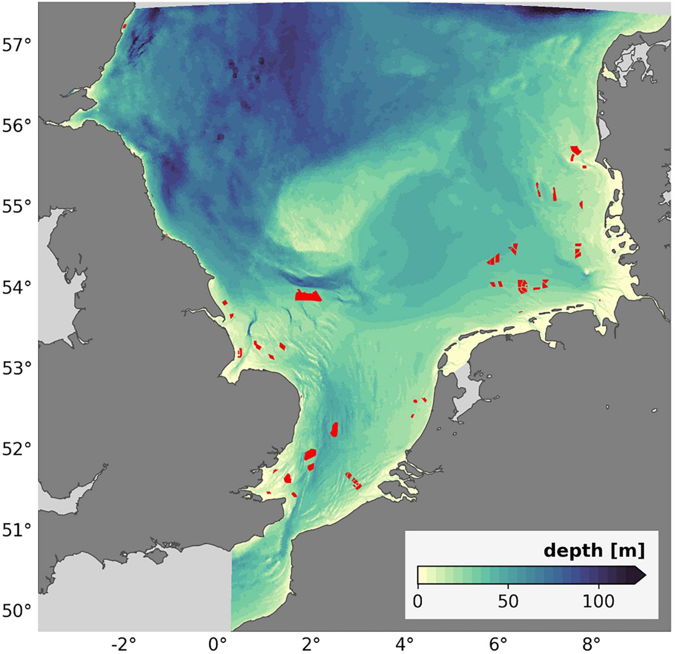
Figure 1. Bathymetry of the model domain (data downloaded from https://www.emodnet-bathymetry.eu/, June 2019) and the fully commissioned offshore wind farms in the southern North Sea, which were considered in this study (red polygons; status as of November 3, 2020, data provided by https://www.4coffshore.com/windfarms/).

Atmospheric Wake Parameterization

Over the years, several empirical and analytical models have been developed to parameterize the downstream wake effects in the atmosphere (Jensen, 1983; Frandsen, 1992; Emeis and Frandsen, 1993; Frandsen et al., 2006; Emeis, 2010; Peña and Rathmann, 2014; Shapiro et al., 2019). While trying to describe wake deficit and wake length, most formulations focused on the relative difference between wind speed along the lee side of wind farms and the undisturbed wind flow. For instance, the analytical model proposed by Emeis (2010) considers wind turbines as additional roughness and is based on the equilibrium between momentum extraction by wind turbines and the replenishment of momentum through turbulent fluxes from above. At this, the change in roughness is assumed proportional to the wind turbine drag coefficient and the wind speed at hub height. However, existing wake models, with regard to wind speed reduction, have so far only been developed for the processes at hub height. Due to the vertical changes of the wake pattern (Frandsen et al., 2006; Emeis, 2010; Fitch et al., 2012; Akhtar et al., 2021), the former models can thus not directly be used for processes near the sea surface boundary. For this reason, we adjusted former model assumptions based on SAR measurements so that they become applicable for numerical ocean modeling.

In a strongly simplified first order approximation, which neglects dependencies arising from specific wind farm characteristics, we parameterized the wind speed deficits resulting from operating wind farms and reduced the mean wind speed in dependence of the respective wind direction. Other impacts, such as turbulence changes or effects on local weather conditions remain unconsidered.

$u(x,y)=u_0\left(1-\mathrm{△}u\right)(1)$

The parameterization for the downstream wind speed reduction [Eq. (1)] is based on earlier studies (Frandsen, 1992; Frandsen et al., 2006) and alters the undisturbed wind field u₀ by the wind speed deficit Δu. The parameterization is applied in a reference coordinate system, where x is the downstream distance aligned to the prevailing wind direction and y defines the distance from the central wake axis. Accordingly, the deficit Δu(x,y) consist of two components describing the downstream wake recovery and the width of the wake structure.

Wake Recovery

The formulation of the downstream velocity deficit is based on the concept of the model by Emeis (2010) (E10 model). The model is a top-down approach model, meaning that the wind farms are considered as one unit of additional roughness, and describes the wake recovery by an exponential decay function. The E10 model was validated in recent studies, which showed that the exponential approach is able to reproduce airborne measurements of atmospheric wakes appropriately (Cañadillas et al., 2020; Platis et al., 2020, 2021). Similar to recent studies, we use the exponential approach of the E10 model to describe the wind speed deficits on the lee side of wind farms. Here, however, we apply the wake formulation in the spatial domain. At this, the wind speed magnitude is prescribed to decrease the strongest close to the offshore wind farms and recovers exponentially over the downstream distance. In summary, the velocity deficit Δu along the downstream distance x is given by:

$\mathrm{△}u(x)=\mathrm{\alpha }{e}^{-x/\mathrm{\sigma }}(2)$

with α as the maximum relative deficit and σ as the exponential decay constant.

Given that the E10 model is established for turbine wakes at hub height, some adjustments are required for the determination of the wake deficit α and the decay constant σ. The individual values for α and σ, in particular near the sea surface, depend on complex relations between multiple aspects, such as the wind field, atmospheric stability, vertical momentum fluxes and wind farm density as well as the wind turbine drag. By the knowledge of the authors of this manuscript, there is so far no empirical or analytical formulation, which either considers these aspects or provides respective values for wind deficit and wake length. Thus, we selected typical mean values for α and σ based on measurements of recent studies (Table 1) and computed SAR data statistics (Figure 2). Thereby, the decay constant σ is defined by the wake length.

TABLE 1

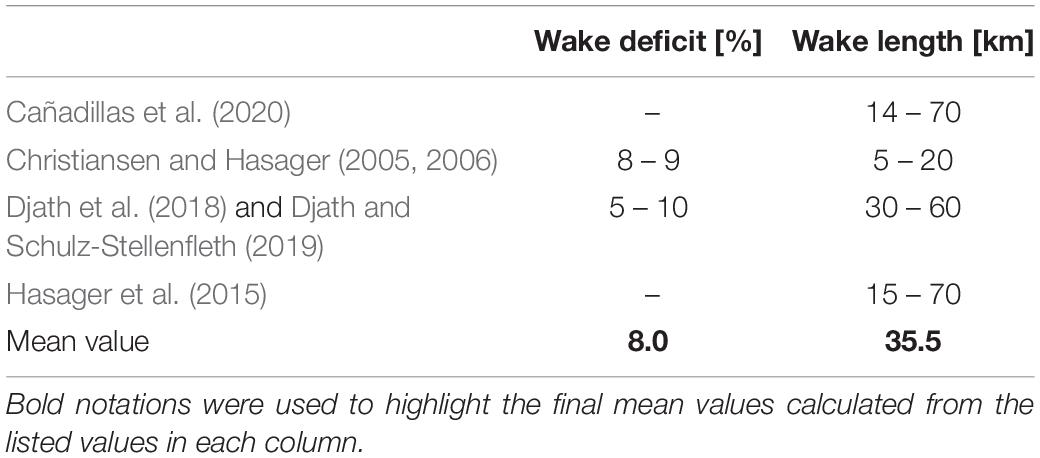
Table 1. Compilation of wind speed deficit α and wake length σ observations of satellite SAR and airborne measurements.

FIGURE 2

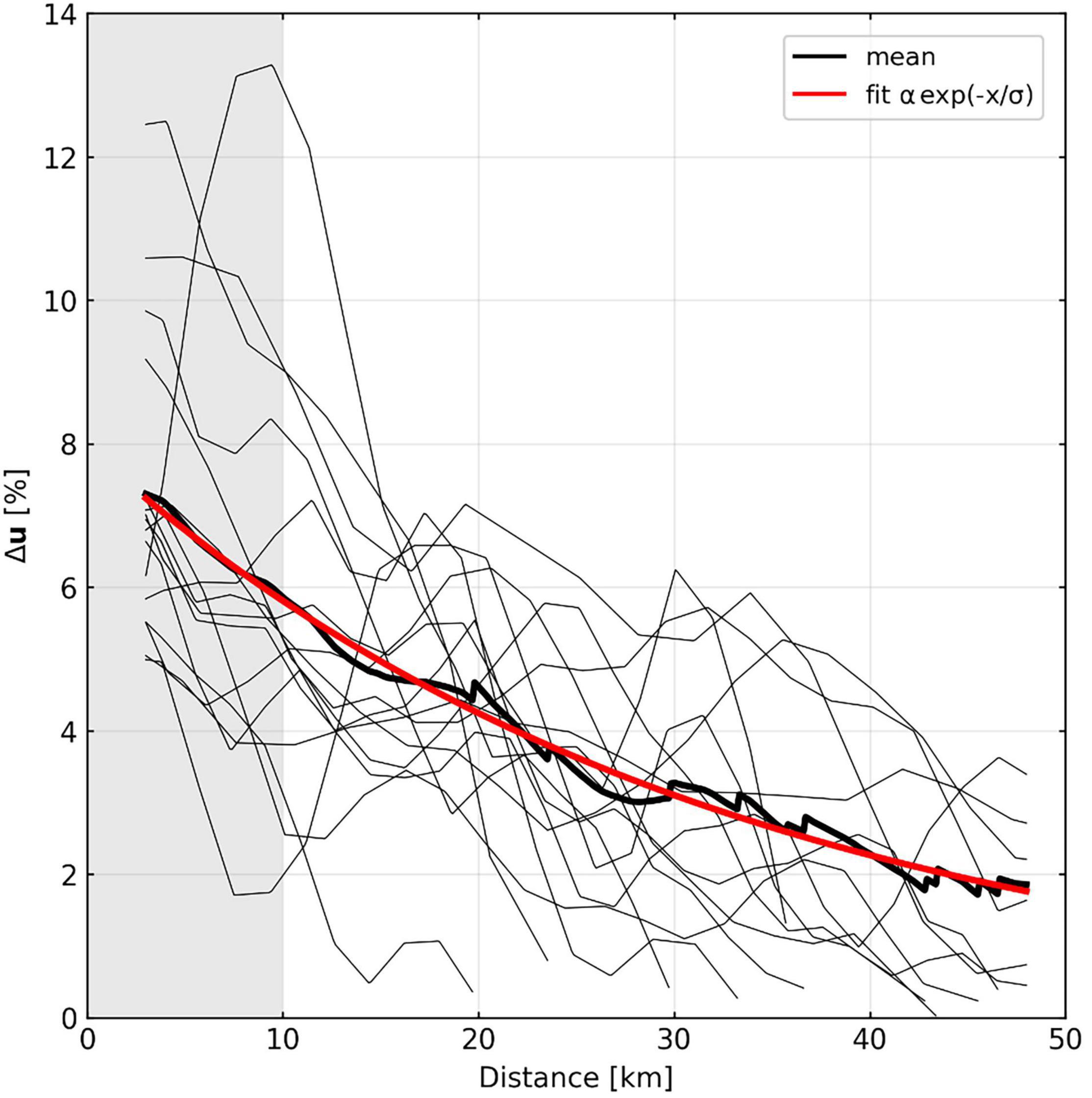
Figure 2. Velocity deficit curves derived from SAR measurements for isolated wake cases at the Global Tech wind farm (thin black lines). The thick black line indicates the average velocity deficit. The red curve corresponds to the best fit of the velocity deficit considering an exponential downstream wake recovery formulation [Eq. (2)], with α = 7.5% and σ = 32 km.

For the SAR data statistics, we utilized latest data sets from Copernicus Sentinel 1 (downloaded April 2019)¹, which consisted of satellite SAR Sentinel1-A and Sentinel1-B data from the period June 2016 to March 2019. We focused on the wind farm Global Tech in the German Bight, which is composed of 80 turbines, and considered wakes from all wind directions, except for cases of superposition of wakes from neighboring wind farms. The velocity deficits were computed using the 10-m wind field from the Synthetic Aperture Radar (SAR). Indeed, SAR technology demonstrated its ability of measuring the surface winds at fine resolution. Thereby, the changes in surface roughness caused by the perturbation of wind speed are captured by the SAR system and modify the Normalized Radar Cross Section (NRCS), which is measured by the satellite. With this, the 10-m surface wind speed is derived from the surface roughness using a geophysical model function CMOD5N (Hersbach et al., 2007) and velocity deficits can be calculated relative to the undisturbed wind field. A detailed description of how to obtain wind speed deficits from satellite SAR data can be found in Djath et al. (2018); Djath and Schulz-Stellenfleth (2019).

In total, the SAR data set resulted in 16 undisturbed wake cases exceeding 15 km length, which are shown in Figure 2. The wake measurements show the highest deficits in the first kilometers behind the wind farm, which decrease over the downstream distance. For the set of profiles, the mean velocity deficit was calculated and fitted to the exponential wake recovery function [Eq. (2)] using the least square method. The exponential fit led to values for α and σ of 7.5% and 32 km, respectively. However, the estimated values for the wake dimension apply primarily for the offshore wind farm Global Tech and might vary due to different wind farm arrays or atmospheric conditions. Thus, we ultimately selected reasonable values of α = 8% and σ = 30 km for the simplified wake parameterization of an undisturbed wake structure. This assumption is supported by earlier studies (Table 1), as the estimated wake deficit and length agree with the mean of previous sea surface wake observations.

Wake Cross-Sectional Shape

The cross-sectional shape of an atmospheric wake can be described by a symmetric exponential function, which is scaled by the characteristic wind farm width L. This assumption was validated in recent airborne measurements, where several wind speed profiles were measured perpendicular to the wake at hub height and fitted to a Gaussian function (Cañadillas et al., 2020). However, Djath and Schulz-Stellenfleth (2019) indicated that the cross-sectional shape of a wake at 10-m height is likely more distinct toward the wake edges. Hence, we chose an exponential decay constant of γ = L/3, in order to narrow the wake cross section at sea surface height in comparison to the hub height assumption. As for the former studies, L describes the wind farm width with respect to the respective wind direction and is calculated for each wind farm individually.

$\mathrm{△}u(y)=e^{-{\left(y/\mathrm{\gamma }\right)}^2}(3)$

The adjusted Gaussian function [Eq. (3)] produces similar cross-sectional shapes to the Kaiser window function, proposed by Djath and Schulz-Stellenfleth (2019), and strikes a balance between the recent cross shape proposals.

Model Description

Model Setup

Due to their spatial extension, atmospheric wakes affect both the small-scale processes near the wind farms and the larger-scale processes in the vicinity of the wind farms. In order to model the cross-scale wake effects, we developed a model setup, which enables the simultaneous resolution of large-scale ocean dynamics and smaller-scale processes near offshore wind farms. For this purpose, we used the Semi-implicit Cross-scale Hydroscience Integrated System Model [SCHISM, Zhang et al. (2016b)]. The SCHISM model is a hydrostatic model grounded on unstructured horizontal grids, which uses Reynolds-averaged Navier-Stokes equations based on the Boussinesq approximation. The model solves transport equations with a second-order Total Variation Diminishing (TVD) advection scheme and applies a higher-order Eulerian-Lagrangian method for momentum advection. At this, it uses semi-implicit time stepping and a hybrid finite-element/finite-volume formulation. A more detailed description of the SCHISM model and its capacities can be found in Zhang et al. (2016a,b).

Our model region covers the North Sea extending laterally from the British Channel in the South to the Norwegian trench in the North and thereby includes the major areas of current offshore wind energy production in the North Sea (Figure 1). The model setup includes the highly resolved coastlines as well as major islands and river estuaries of the surrounding mainland. We used a depth-depending horizontal grid cell resolution for the triangular unstructured grid, ranging from 500 m in shallow coastal areas to 5,000 m in the deep open sea. In total, the grid has approximately 161 K nodes and 311 K triangles. In the vertical direction, we applied a flexible LSC² [Localized Sigma Coordinates with Shaved Cells, Zhang et al. (2015)] grid, which is composed of a depth-depending number of localized sigma coordinates and considers in total 40 depth levels. The layer thickness increases gradually from about 2 m in the surface layers to 10 m in levels below 100 m depth.

At the open boundaries, the model was forced by the North-West European shelf ocean physics reanalysis data from the Copernicus Marine Service (downloaded July 2019)², which we interpolated for time series of elevation, velocity, temperature, and salinity. Additionally, we prescribed tidal amplitudes and phases of eight tidal constituents (M₂, S₂, K₂, N₂, K₁, O₁, Q₁, and P₁) from the data-assimilative HAMTIDE model (Taguchi et al., 2014). For the atmospheric forcing, the coastDat-3 COSMO-CLM ERA interim atmospheric reconstruction (HZG, 2017) was applied, while daily river discharge values were provided by the mesoscale Hydrologic Model [mHM, Samaniego et al. (2010), Kumar et al. (2013)] using the E-OBS18 temperature and precipitation data set (Cornes et al., 2018). Werner et al. (in prep.) will provide a more detailed description of the discharge data. Bottom roughness was set to 0.1 mm and we used a vertical background diffusivity of 10^–6 m²/s. Initial conditions were interpolated from the same data sets as the boundary forcing data.

Model Simulation

After an initial spin-up simulation of two and a half years, we simulated offshore wind farm operation for the summer period of 2013 (May to September) in a subsequent model run. As the characteristic “flushing time” of the North Sea is about one year (Otto et al., 1990), the short spin-up period can be deemed sufficient for the model area. While the period of the simulations was generally chosen based on data availability, the simulation period for the wind farm simulations was chosen to ensure mostly stable atmospheric conditions, which enable the formation of large-scale wake structures. Thus, the simulations allow the investigation of the impact of wind farm wakes on the summer stratification. For all simulations, an implicit time step of 120 s was used and the daily mean was calculated for the output data.

The wind farm simulation took into account the recent state of offshore wind farm production within the model domain (see Figure 1). However, the wind farms were only considered via the implemented wake parameterization and were not represented physically in the horizontal grid. For the simulation, we applied the wake parameterization to the wind field interpolated onto the horizontal model grid and reduced the horizontal components of the wind speed respectively. Specifically, the wind speed on downstream grid points was iteratively reduced for each wind farm. While the parameterization modified the downstream wind field at each time step of the simulation, we considered a wind speed limitation (cut-in and cut-out speed) for wind farm operation in the wake model. For this, we used a typical wind speed range of 3–25 m/s at hub height, which inhibits wake generation for too weak and too strong wind speeds.

We enhanced the horizontal grid cell resolution in the wind farm simulation to resolve hydrodynamic processes near the offshore wind farms sufficiently and to provide highly resolved wake effects. The grid optimization involved a boundary layer of 30 km around each wind farm polygon with a grid cell size of 1,000 m (see Figure 3). In addition, a high-resolution zone with a grid cell size of 500 m was defined in the first five kilometers around each wind farm, where the wind deficits are most pronounced. In total, the adjusted horizontal grid of the wind farm simulation resulted in approximately 278 K nodes and 544 K triangles.

FIGURE 3

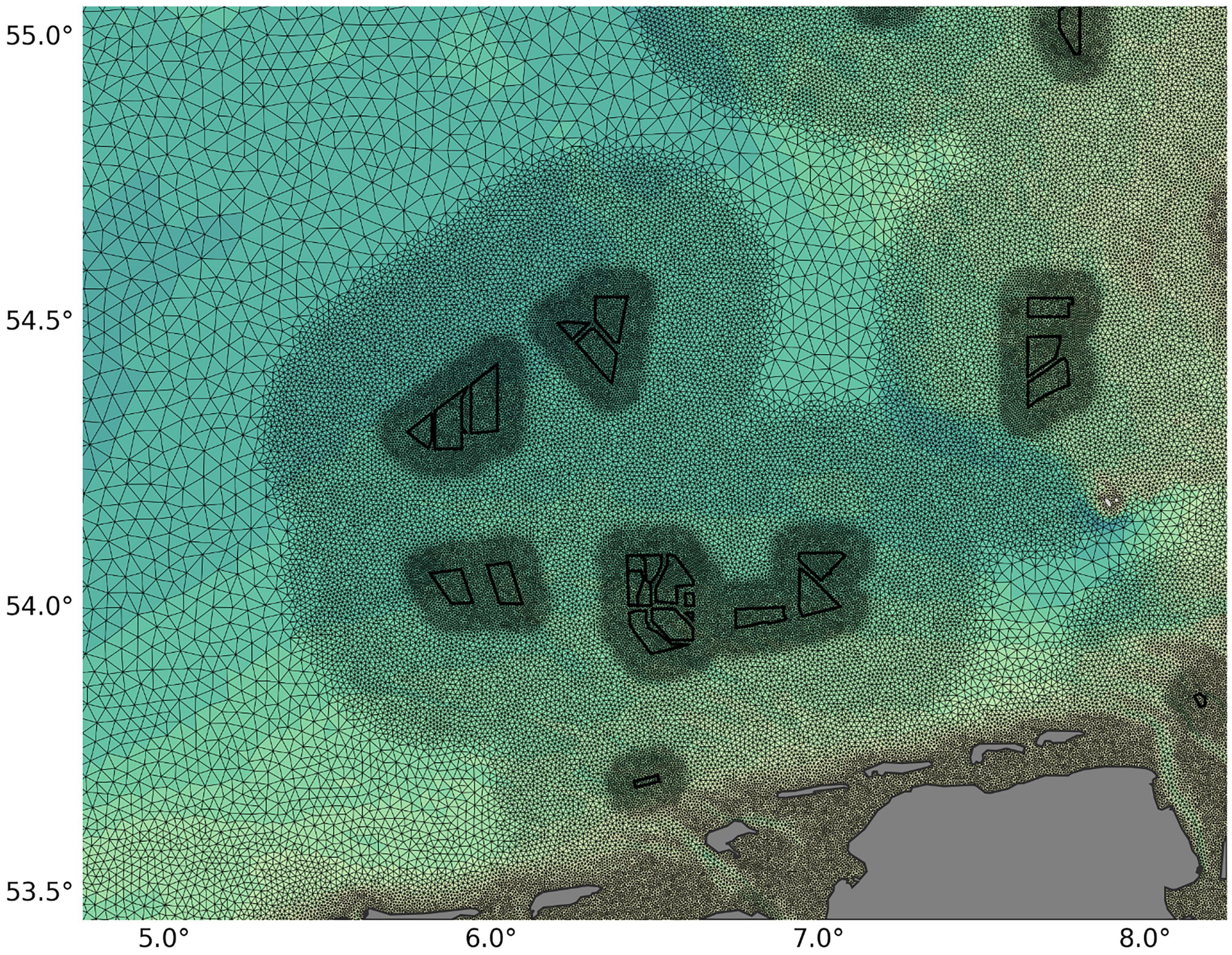
Figure 3. Example of the horizontal grid cell resolution at wind farm polygons (black) for the wind farm simulations.

In order to compare differences between the wake-exposed North Sea and the reference case we ran the summer period twice, with and without wind farm parameterization. For both cases, the enhanced grid cell resolution was applied.

Model Validation

In order to validate the model simulations, temperature and salinity values were downloaded from the ICES database (downloaded March 2020)³ for the period from January 2012 to December 2013. The observational data set consists of about 3,250 stations, at which temperature and salinity samples were collected at different water levels. For the validation, we calculated the depth-averaged data to avoid uncertainties in depth levels and compared it to the respective daily-mean values of the spin-up simulation, which forms the basis of the wind farm scenarios.

We utilized a Taylor diagram (Taylor, 2001) to display the statistics of our model simulations. The diagram is based on the law of cosine and quantifies differences between observation and model by the centered root mean square difference E’ and the correlation coefficient R. The root mean square difference and the correlation coefficient are calculated as:

$E^{\prime }={\left(\frac{1}{N}\sum _{n=1}^N{\left(\left(O_n-\overline{O}\right)-\left(M_n-\overline{M}\right)\right)}^2\right)}^{\frac{1}{2}}(4)$

and

$R=\frac{\frac{1}{N}{\sum }_{n=1}^N\left(M_n-{\overline{M}}_n\right)\left(O_n-{\overline{O}}_n\right)}{{\mathrm{\sigma }}_M{\mathrm{\sigma }}_O}(5)$

with ${\mathrm{\sigma }}_X=\sqrt{\frac{1}{N}{\sum }_{n=1}^N{\left(X-\overline{X}\right)}^2}$ as the standard deviation, M as model data and O as observation data.

Similar to Daewel and Schrum (2013), we subdivided our model domain into different validation areas based on their physical characteristics (Figure 4A). Here, we focused on five main characteristic regions: The Atlantic inflow area (D), the British coast (E), the shallow tidal-impacted coastal areas connected to the Wadden Sea (F&G), the Baltic in- and outflow area (H) and the seasonally stratified central North Sea (K&L). For the statistics, we treated each region individually.

FIGURE 4

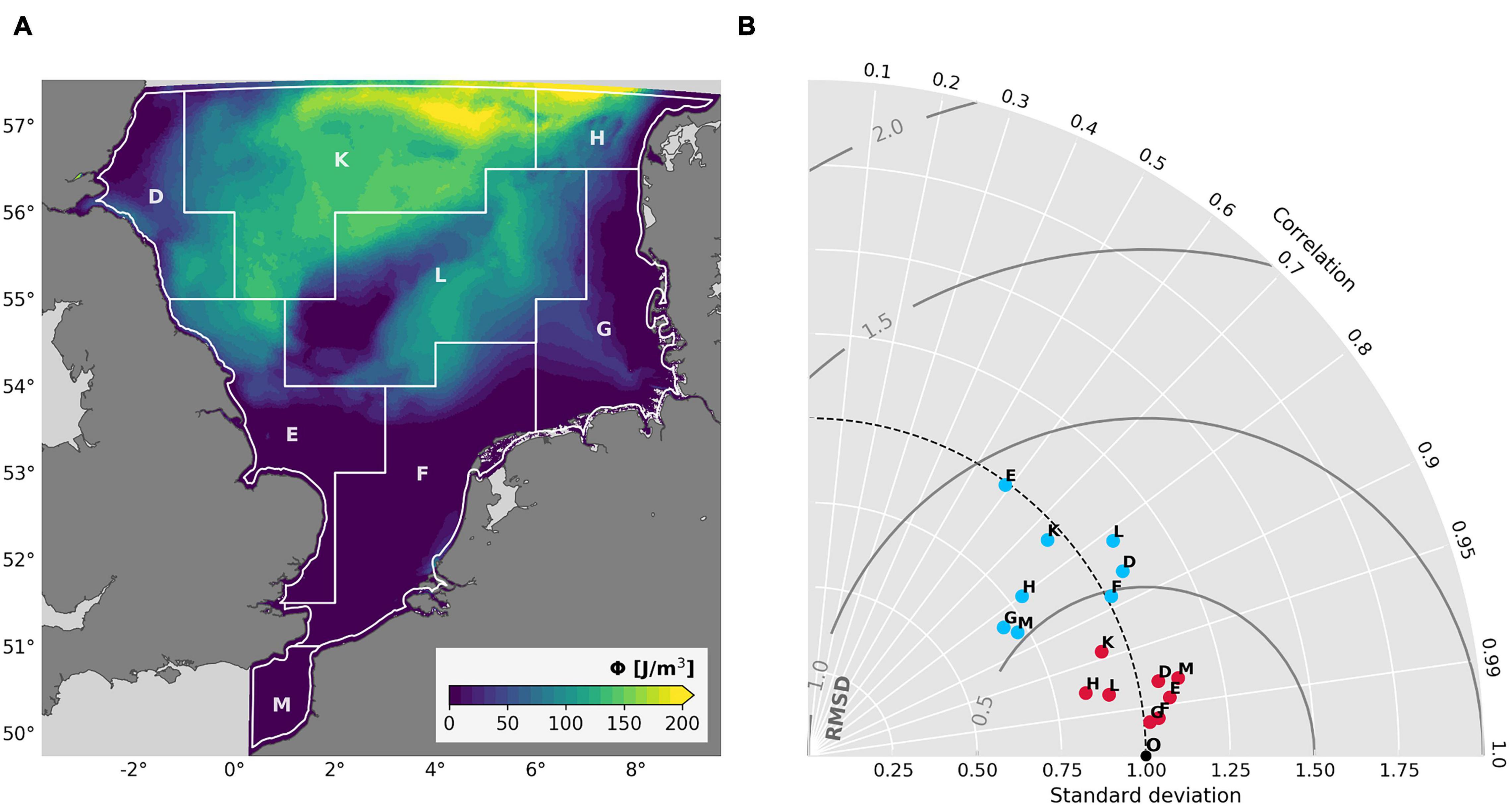
Figure 4. Validation of the spin-up simulation: (A) Mean potential energy anomaly in August and the characteristic subareas for the model validation. Area separation was applied according to Daewel and Schrum (2013). (B) Taylor diagram for depth-averaged temperature (red dots) and salinity (blue dots) in the different subdivisions of the model domain with respect to the observation statistics. O, observation data.

The calculated Taylor diagram (Figure 4B) shows high correlation (R > 0.9) between the spin-up simulation and the observations for sea surface temperatures. Seven out of eight subareas exhibit correlation coefficients above 0.95, from which the areas connected to the Wadden Sea (F&G) show the highest values (R > 0.99). Only region K, the deep central North Sea area, shows a slightly lower correlation, which is probably due to the influence of the large northern open boundary of the model domain. Surface salinity has a lower, but still decent, overall agreement between the model and the observational data. Most coefficients range between 0.8 and 0.9, whereas only region E, the British coast region, and again region K show lower correlations. Generally, the lower correlation in salinity likely results from the comparison of daily-mean model data and instantaneous observational data, as we observe strong fluctuations in the fresh water inflow due to the tidal signal. Averaging the model data results in attenuated tidal fluctuations and thus lower correlation to the instantaneous values of the observational data. The British coastal area in particular, has strong tidal amplitudes, which could explain the particularly low correlation in region E.

In general, the model proves a sufficient correlation to the in-situ measurements and is able to reproduce seasonal stratification in the southern North Sea (Figure 4A). The pattern of the mean potential energy anomaly, which is a gravitational-based measure of stratification strength of the water column (Simpson and Bowers, 1981), shows expected characteristics, such as strong stratification in the deep central North Sea as well as mixing fronts around the shallow Dogger Bank and along the tidal-impacted Wadden Sea area. Thereby, the stratification patterns (exemplarily shown for August, Figure 4A) agree well with results of former North Sea studies (Schrum et al., 2003; Holt and Proctor, 2008) considering that magnitude and spatial dimension of summer stratification vary between years (Schrum et al., 2003).

Results and Discussion

The analysis of wake effects in this manuscript concentrates on general processes related to the transfer of atmospheric momentum into the water column and associated mean changes in horizontal currents and stratification. In order to emphasize the induced changes during the summer period of 2013, wake effects are shown as the differences between the case of wind farm operation and the case without offshore wind farms in the southern North Sea. In the following, the data is primarily depicted as monthly means, while only a selection of figures is depicted in the analysis. For further insights on the monthly means, see Supplementary Figures A1–A6.

Spatial and Temporal Variability in Hydrodynamics

The implemented wake parameterization iteratively generates leeward wind speed reductions at each time step of the simulation. Despite the constant values for the wake deficit and wake length prescribed by the wake model, the resulting wake structures vary individually in size and intensity due to the different sizes of the respective wind farm arrays and due to superposition of neighboring wakes. A snapshot of a strong wind event during the simulation and an example of the associated downstream velocity deficits are depicted in Figure 5A. The emerging wakes extend along the present wind field and show comparable patterns to recent satellite SAR wake observations (Djath et al., 2018; Siedersleben et al., 2018). At this, the simulated wakes exhibit relative deficits around 10% in short downstream distances, which agrees with the observations of recent satellite SAR data (Table 1). The strongest reductions in wind speed are observed in densely built areas of the domain, in particular in the German Bight. Although the wake model prescribed a constant deficit of 8%, superposition of neighboring wakes in densely built areas results in even higher velocity deficits of up to 15%, as multiple wind farms affect the wind speed.

FIGURE 5

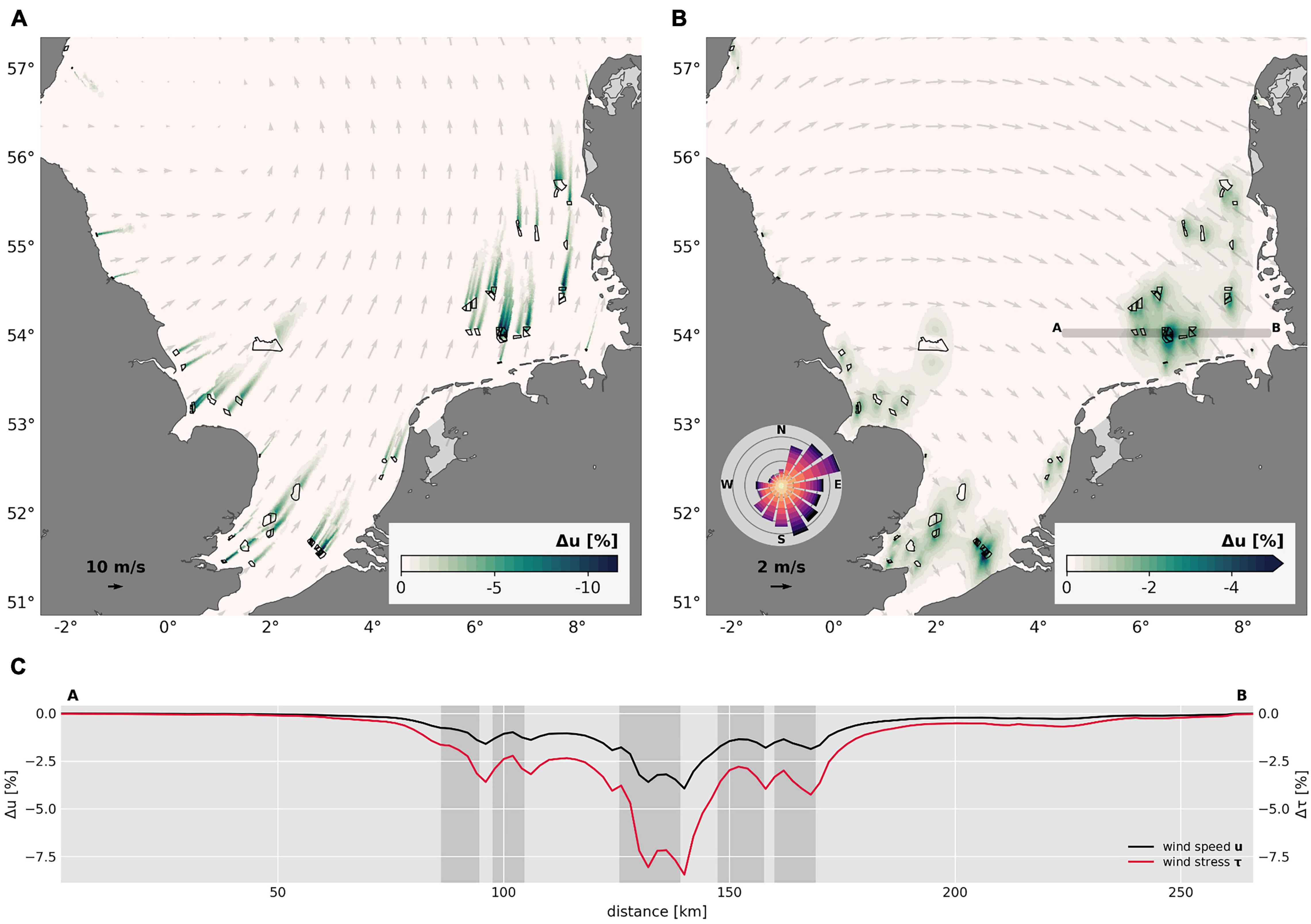
Figure 5. Relative changes in mean wind speed (u): Instantaneous changes for a strong wind event on 10 May 2013 (A) and mean wind speed changes for the period of May – September 2013 (B). Gray arrows indicate mean wind direction. The wind rose indicates the direction in which the wind blew (color range between 1 and 12 m/s). (C) Relative changes in wind speed (u) and wind stress (τ) along transect (A,B). Gray areas indicate locations of offshore wind farms.

As a result of constantly changing wind directions, pronounced wake patterns disappear when averaging over time and shape continuous zones of reduced wind speed around the respective wind farms. Thereby, the German Bight is the most affected region of the model domain, as a large number of current offshore wind farms is located off the Danish, German and Dutch coast. The mean deficits in wind speed of the 5 months of simulation are shown in Figure 5B. The deficits were calculated for the absolute values of the wind vectors. Figure 5B shows that the mean wind speed deficits primarily adapt to the predominant wind field during the simulation period, which here points into eastward direction. Furthermore, strong wind events, which might differ from the mean wind directions, can influence the shape of the wind speed anomalies particularly in areas of weaker winds (e.g., the British coast). Between May and September, the total absolute mean changes in wind speed range on average around 1–2% relative to the mean undisturbed wind field and can reach even beyond 5% in areas of clustered wind farms, like the Southern Bight or German Bight. Compared to the mean undisturbed wind speeds, which are between 5.0 and 7.0 m/s, the deficits account for an order of magnitude of about 0.1 m/s and range between 0.1 and 0.4 m/s. The order of magnitude is in agreement with recent atmospheric modeling results of Akhtar et al. (2021), where deficits near the sea surface range around 0.5 m/s during the summer months, considering that Akhtar et al. (2021) applied more influential future wind farm scenarios. Nevertheless, here, with regard to the interpretation of the magnitude of mean wind speed perturbations, the supposed over- and underestimation of the wake dimension due to the prescribed constant wake parameters should be taken into account.

The wake-induced anomalies in wind speed cover large areas around the actual wind farm locations. Consequently, wide areas are affected by reduced shear forcing and reduced vertical momentum fluxes at the sea surface boundary. This becomes particularly apparent looking at a cross section through the strongly influenced southeastern part of the German Bight (Figure 5C). Along the cross section the percentage change in wind speed and wind stress is shown relative to the undisturbed values from the scenario without wind farm operation. Both, wind speed and wind stress, exhibit continuous deficits over several tens of kilometers, which do not fully recover in between adjacent wind farms and are particularly strong in the case of superimposed wakes. Thereby, the impact on the wind stress, which is the decisive factor for vertical air-sea exchange, is about twice as high in percentage as for the mean wind speed. Within the wind farm areas deficits slightly recover, since the wake parameterization reduces wind speed only downstream of wind farms. A similar pattern of the continuous influence arising from superimposed wakes was also shown by recent high-resolution atmospheric modeling of offshore wind farm effects (Akhtar et al., 2021), where moreover the effect on offshore wind energy production itself was addressed.

In this study, the focus is on the large regions of attenuated wind forcing and related impact on the marine environment. In the shallow southern North Sea, where for the most part wind determines the general circulation (Sündermann and Pohlmann, 2011), the reduction of wind speed and associated wind stress results in substantial changes of the residual circulation. As less shear force is acting on the sea surface in areas around the wind farms, vertical momentum fluxes become attenuated and less momentum is transferred from the atmosphere into the ocean. This entails potential changes in wave formation and horizontal surface velocity but also potentially reduces turbulence within the surface mixed layer and impacts stratification.

Figure 6A depicts the mean changes in horizontal surface velocity after the first month of wind farm operation. The pattern shows expected lateral gradients in the horizontal currents as a result of the reduced wind stress behind offshore wind farms. At this, negative anomalies arise at wind farms in direct correlation to the downstream wind speed deficits of the predominant mean wind field (Supplementary Figure A1). In consideration of the prescribed wake intensity (8% deficit, 30 km length) and the prevailing wind speeds, the deficits in surface current speed range around −0.0025 m/s and exhibit peak values beyond −0.005 m/s. While the order of magnitude agrees with former wind farm studies (Ludewig, 2015), the velocity changes account for up to 5% compared to the mean surface residual velocity in May (about 0.1 m/s). The induced changes are up to 10–25% of the interannual and decadal surface velocity variability, as the mean surface velocity in the southern North Sea ranges between 0.11 and 0.13 m/s (Daewel and Schrum, 2017). Consequently, wake-induced anomalies in surface velocity can be quite substantial, considering that instantaneous changes are generally even stronger, and might affect the horizontal transport and eventually the residual currents in areas of wind farm operation significantly.

FIGURE 6

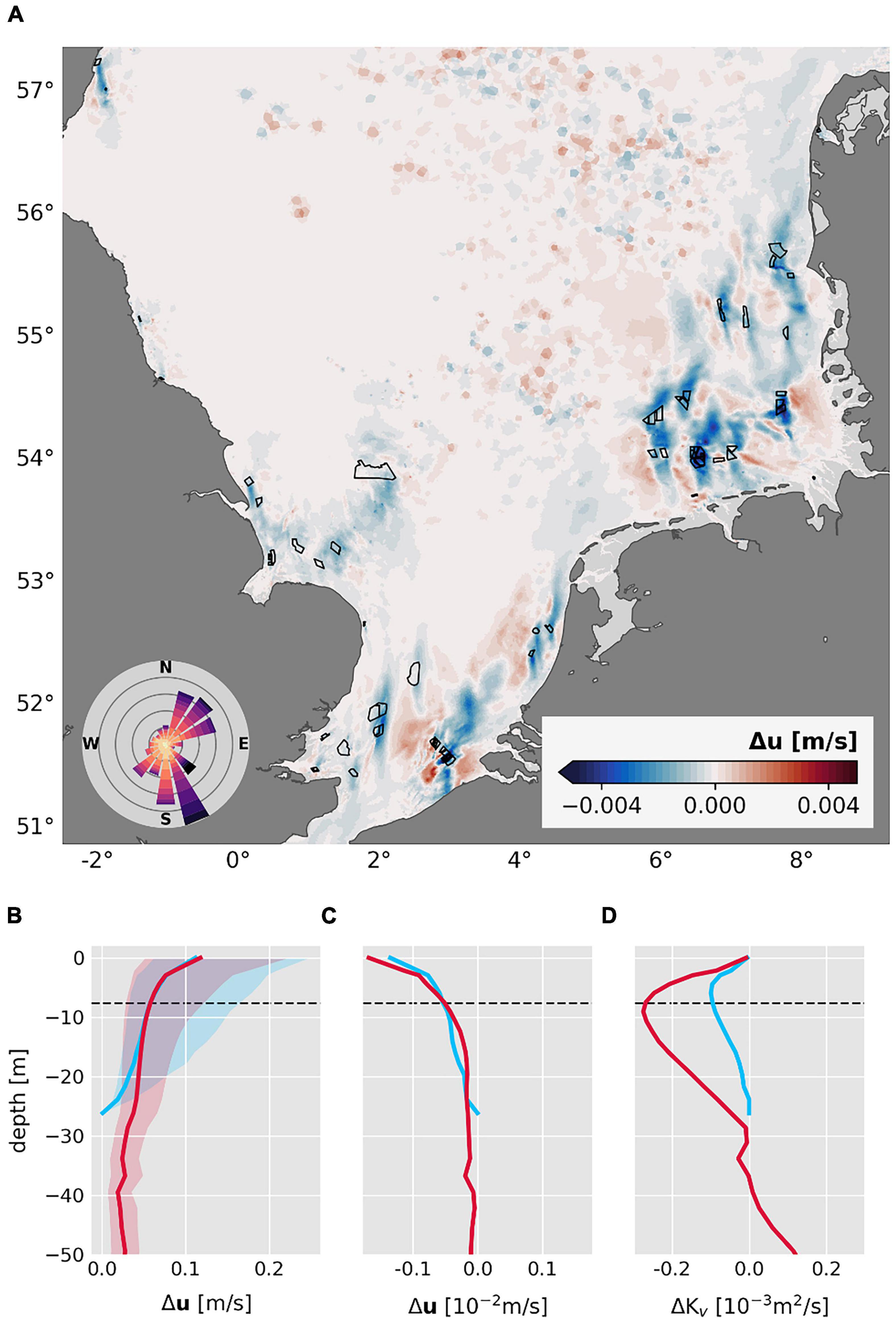
Figure 6. Mean changes in horizontal velocity (u) and mixing rate (K_V). (A) Mean changes in horizontal sea surface velocity for daily mean data in the month of May. Black polygons indicate offshore wind farms. The wind rose indicates the direction in which the wind blew (color range between 1 and 12 m/s). Mean vertical profiles for the mean horizontal velocity (B), the mean changes in horizontal velocity (C), and the mean changes in mixing rate (D) at wind farms for the month of May 2013. Filled envelopes in panel (B) demonstrate the temporal variability during May. Dashed lines indicate location of the mixed layer depth. For the profiles, grid points within 5 km around each wind farm were considered. Profiles are divided into deep (z ≥ 25 m, red lines) and shallow (z < 25 m, blue lines) water depths.

In order to evaluate the impact of the wind stress reduction on the vertical structure of the horizontal momentum, mean vertical profiles at the wind farm locations are depicted in Figures 6B–D. For the vertical profiles, we used grid points only located within a radius of about 5 km around each wind farm and calculated the average monthly mean changes within the water column. Thereby, shallow (z < 25 m) and deep (z ≥ 25 m) waters were treated separately, as they show different dynamics related to the wind shear.

Figure 6B shows the average horizontal velocity profile at the offshore wind farm locations and the temporal variability during the month of May. As for the entire southern North Sea, the mean surface velocity at the wind farm locations is about 0.12 m/s, which agrees with the results of Daewel and Schrum (2017). However, the variability of surface velocity itself reaches up to 0.15 m/s within May and is much stronger than the interannual variability. In terms of wake-induced alterations in the horizontal velocity, the wind farm profiles show the strongest changes occurring at the sea surface boundary, where the impact by the wind speed reduction is most powerful (Figure 6C). Here, the maximum values range around -0.002 m/s at the sea surface, which is lower than the maximum changes in Figure 6A, since the wind farm locations are less affected by wakes than the areas in downstream direction. The order of magnitude of the changes accounts for about 2% of the mean horizontal velocity profiles at the wind farms as well as of the velocity variability over the month of May (Figure 6B). The wake-induced changes in horizontal velocity are more pronounced in deeper waters than in shallow coastal areas. Thereby, deep waters exhibit a strong vertical gradient between the surface and deeper layers, which emphasizes that particularly the wind-driven surface mixed layer is affected by the wind stress deficits. Nevertheless, the impact of the momentum deficit also cascades downward into deeper layers and diminishes toward the sea floor.

In addition to the perturbations in velocity, the attenuation of vertical momentum fluxes results in the associated reduction of turbulent mixing inside the surface mixed layer (Figure 6D). Here, as a measure for the mixing rate, we depict the vertical eddy diffusivity K_v. The profiles exhibit a reduced mixing rate over the entire water column. As for the horizontal velocity, the deficits in mixing are more pronounced in deep waters than in well-mixed shallow waters, which is likely favored by influence of the bottom mixed layer in shallow depths. In both cases, the strongest deficits occur near the pycnocline depth. While, in general, the apparent decrease in mean turbulent mixing implies a less turbulent water column, the maximum deficits near the mixed layer depth indicate a shallower surface mixed layer at offshore wind farms. This implies that the wind wakes counteract to the recently identified effects of Kármán vortices and turbulent wakes created by the pile structures of wind turbines, which are responsible for additional mixing in downstream direction (Carpenter et al., 2016; Grashorn and Stanev, 2016; Schultze et al., 2020). Thus, offshore wind farms induce counteracting processes, namely the reduction of horizontal momentum and the generation of turbulence, due to the wind turbine rotors and wind turbine foundations, respectively. However, the counteracting processes emerge on different spatial scales, since the pile effects remain primarily within the wind farm areas (Schultze et al., 2020).

Earlier studies showed the impact of the wind stress reduction on the sea surface elevation at offshore wind farms (Broström, 2008; Paskyabi and Fer, 2012; Ludewig, 2015). The studies demonstrated the formation of up- and downwelling dipoles under constant wind directions, which extend several kilometers around the wind farms. In a realistic model setup, such as we used, however, the wind field changes continuously over time and individual dipole patterns are expected to superimpose or mitigate, depending on the respective wind field. Figure 7A depicts the resulting mean surface pattern in August. Indeed, the changes in elevation superimpose into large coherent patterns of positive and negative anomalies, which smoothly merge into each other. Thereby, large-scale dipoles with spatial dimensions of up to hundreds of kilometers emerge in the wind farm regions and in particular in the German Bight area, where superposition and thus amplification of wake effects occurs most frequently. Compared to the mean wind field in August, which points into eastward direction (see Supplementary Figure A1D), the surface elevation dipoles exhibit their positive amplitude roughly on the windward side of wind farm areas and their negative amplitudes to the lee side. This might indicate a damming effect of wind-driven horizontal flow by the offshore wind farms.

FIGURE 7

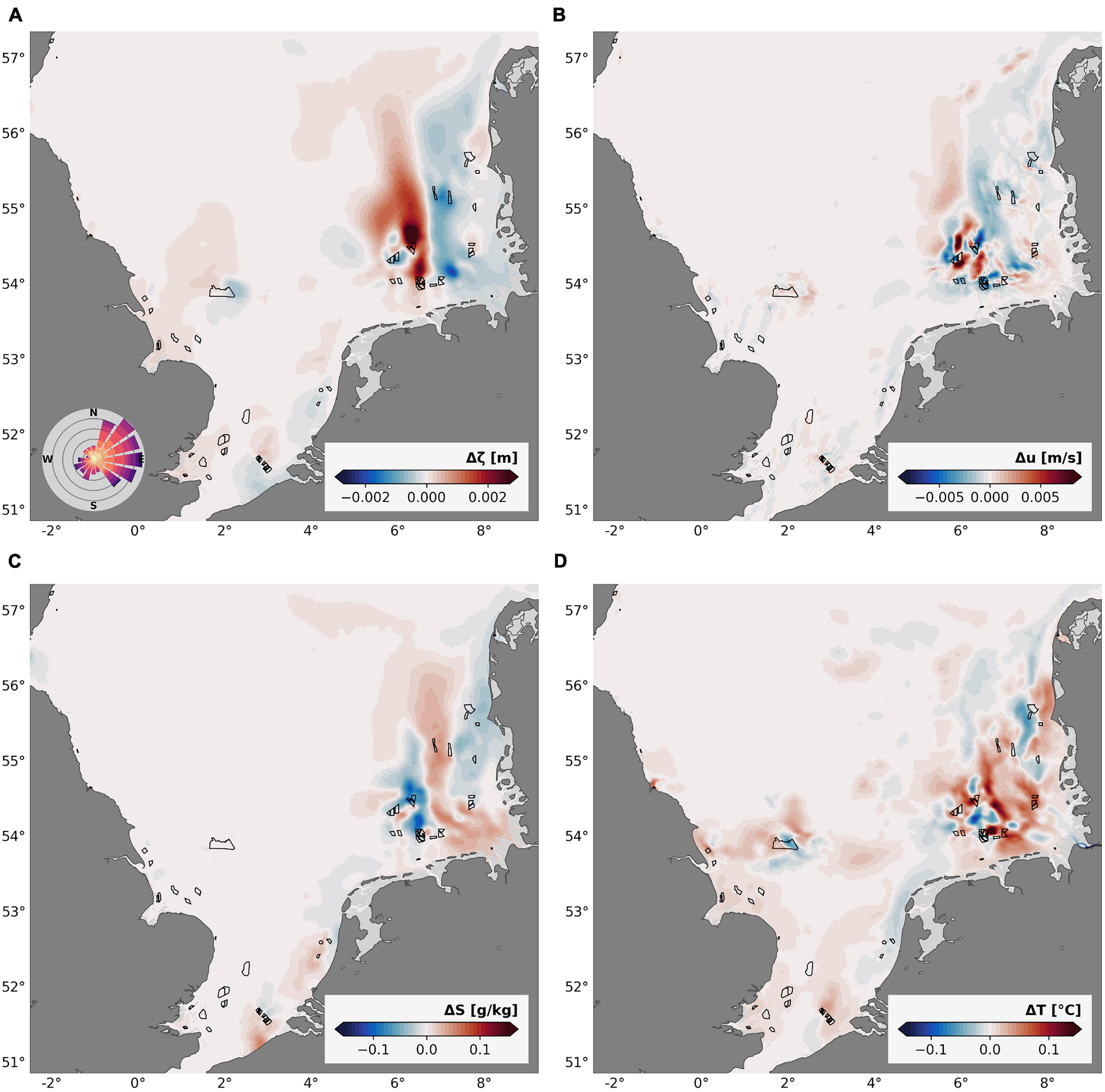
Figure 7. Mean changes in sea surface elevation ζ (A), depth-averaged velocity u (B), sea surface salinity S (C), and sea surface temperature T (D) for the month of August 2013. Black polygons indicate offshore wind farms. The wind rose indicates the direction in which the wind blew (color range between 1 and 12 m/s).

The changes in sea surface elevation show a clear correlation to the anomalies in mean depth-averaged velocity, which resemble the dipole pattern in the German Bight in August (Figure 7B). At this, the mean depth-averaged velocity changes range between ± 0.001 and 0.005 m/s and reach on maximum nearly 0.01 m/s. These changes are up to twice as strong as the wind stress related velocity changes at the sea surface in May (Figure 6A) and account for up to 10% of the mean horizontal flow velocity in the German Bight. In percentage terms, such perturbations of the flow pattern are quite significant, as they are comparable to the potential changes due to climate change (Mathis and Pohlmann, 2014; Schrum et al., 2016) and may affect the residual currents as well as the gradients of the mean sea surface elevation in the German Bight area.

The relation between horizontal flow perturbations and sea level anomalies becomes more apparent by zooming in on the dipole structure in the German Bight specifically (Figures 8A,B). The figures illustrate the vector field of the mean depth-averaged horizontal velocity changes, in addition to the mean sea level and velocity changes in August. Figure 8A shows that the positive and negative mean sea level anomalies are clearly related to attenuated or enhanced horizontal flow velocities. At this, the sea level sinks in regions of increased flow velocity, while the sea level rises due to damming in regions of reduced flow velocities. This applies specifically to the large-scale dipole pattern. In the center of the German Bight, where the perturbations are most pronounced, the mean changes in sea surface elevation reach orders of magnitude of around ± 2 mm and result in spatial gradients of up to 4 mm over a distance of several tens of kilometers. These magnitudes are weak, compared to the local tidal variability and account for about 1–10% of the mean surface elevation variability in the German Bight, which varies by around 0.05–0.10 m over the respective spatial scales. However, the occurrence of such strong sea level gradients can in turn affect the geostrophic balance in the German Bight. Considering the apparent sea level differences of 2–4 mm, the resulting horizontal pressure gradients would affect the predominant circulation pattern by an order of magnitude of about 10^–3 m/s, which is similar to the wake-related changes in horizontal velocity. In fact, these secondary induced perturbations of the geostrophic flow can be seen in the changes of the mean horizontal flow pattern (Figure 8B), where eddy-like structures with associated magnitudes of ± 0.006 m/s emerge in the center of the German Bight. However, these eddy-like structures might also be the result of mean depth-averaged circulation changes, which in turn favor the emergence of up- and downwelling cells.

FIGURE 8

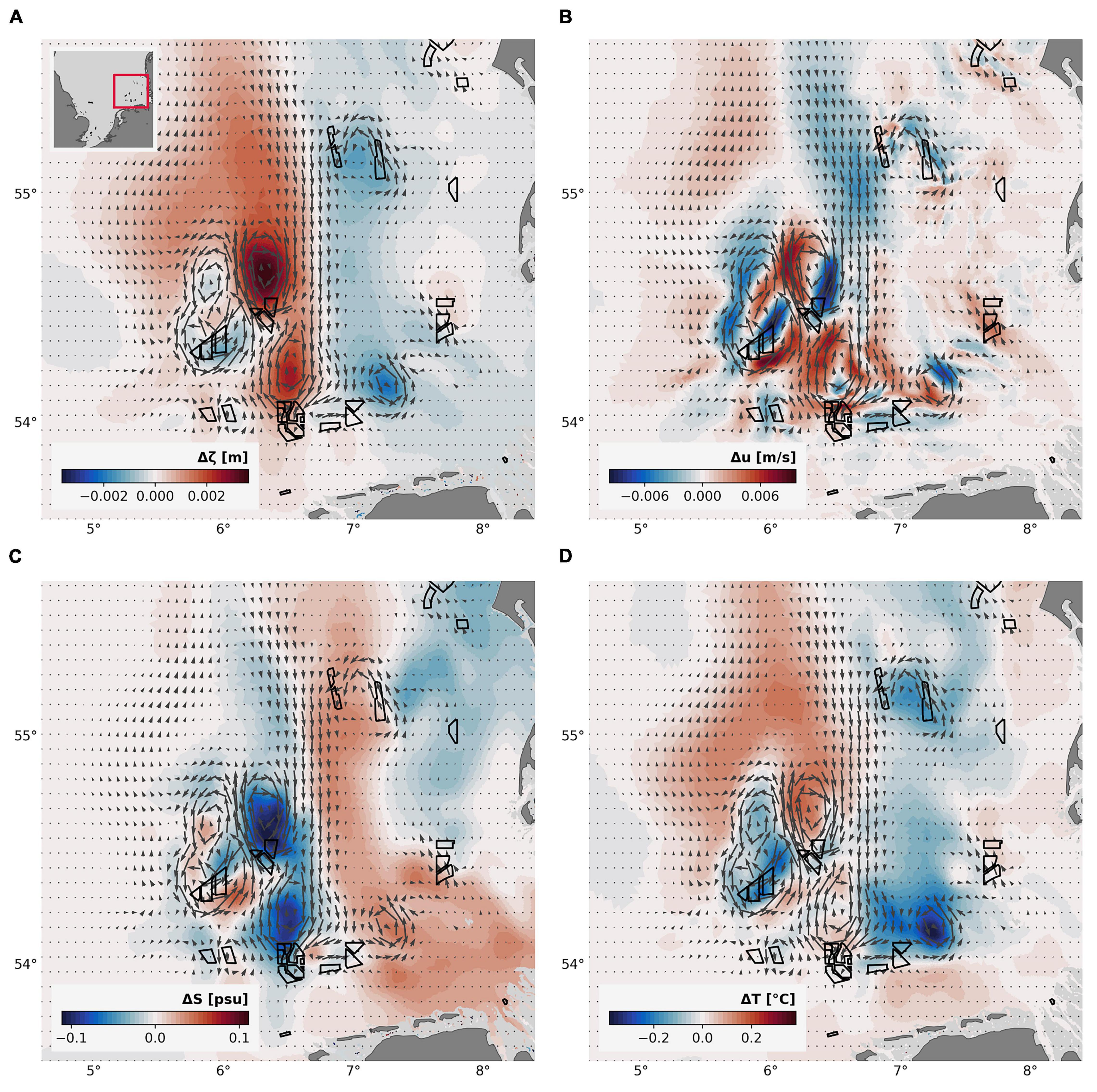
Figure 8. Mean changes in sea surface elevation ζ (A), depth-averaged velocity u (B), depth-averaged salinity S (C), and depth-averaged temperature T (D) in the German Bight for the month of August 2013. The black arrows indicate the direction of the changes in depth-averaged velocity. Black polygons indicate offshore wind farms.

Impact on Stratification

The alterations of the sea level and the horizontal transport suggest changes in the lateral and vertical density fields. In a previous modelling study, Ludewig (2015) observed the occurrence of vertical upward and downward currents at offshore wind farms, which were inversely correlated to the displacements of the sea surface dipole. With sufficient temperature and salinity stratification, the induced vertical flow is expected to result on the one hand in advection of colder and saltier toward the surface and on the other hand in the downward advection of warmer and fresher water within the dipole area. Consequently, the changes in sea surface elevation are accompanied by changes in the vertical temperature and salinity distribution.

Figure 7C depicts the mean sea surface salinity changes in August, where the magnitudes on average range between ± 0.05 g/kg. In the Southern Bight, the presumed correlation between the surface elevation anomalies and the surface salinity changes becomes most apparent. Positive and negative changes in surface salinity agree with the locations of the sea level perturbations and extend several tens of kilometers around the wind farms. At this, saltier surface water occurs in regions of lowered sea level, while surface salinity decreases in regions of elevated sea surface height. In the German Bight however, the large-scale pattern is more complex and does not clearly resemble the specific pattern of the mean sea surface elevation. Here, mean surface salinity decreases within the center of the large sea level dipole and along the shallow Jutland coast. Between the two negative salinity anomalies, salinity increases and the positive anomaly spreads along the fresh water plume from the Elbe estuary.

The mean surface temperature changes show much less agreement to the anomalies in sea surface height (Figure 7D). Instead, it appears that the surface temperature primarily increases in the vicinity of offshore wind farms, which confirms earlier simulations by Ludewig (2015). The apparent surface heating presumably results from the reduction in mixing and is hence directly related to the large-scale wind speed reduction in the atmospheric forcing. Over time, advection and lateral transport likely cause the temperature anomalies to spread over a large scale in the affected areas. Therefore, coherent patterns of increasing mean sea surface temperature are present in areas of wind farm development. At this, mean changes in sea surface temperature are on average around ± 0.02–0.05°C, whereas changes in the German Bight reach even beyond 0.1°C. The large-scale surface heating of up to 0.1°C imitates the effects of climate change, in which an increase in sea surface temperature is also to be expected as a result of the warming of the earth’s atmosphere (Schrum et al., 2016). However, the wake-related changes are about one order of magnitude smaller than the average perturbations due to climatic changes (Schrum et al., 2016). Furthermore, the changes account for a maximum of 10% of the annual and interannual variability of surface temperature in the southern North Sea, which are at least 1.0–1.5°C (Daewel and Schrum, 2017).

Despite the deviations in the surface anomalies, the mean depth-averaged changes in temperature and salinity confirm the assumed correlation between the sea level changes and the changes in the density field in the German Bight (Figures 8C,D). The figures show again the vector plot of the mean depth-averaged horizontal velocity changes, in addition to the mean depth-averaged changes in temperature and salinity in August. For the depth-averaged data, salinity and particularly temperature exhibit stronger changes than for the sea surface with up to ± 0.1 g/kg and ± 0.3°C, respectively. At this, the anomalies show a clear agreement with the vector plot of the depth-averaged velocity changes and with the mean sea level anomalies (see Figure 8A). In particular, the mean temperature changes strongly resemble the sea level alterations (Figure 8D). Nevertheless, for both, temperature and salinity, a notable amplification of the changes occurs due to the eddy-like structures in the horizontal flow anomalies and hence due to the amplified changes in sea level. These changes agree with the presumed correlation between the sea level anomalies and changes in the vertical density distribution and thus with the results of Ludewig (2015). However, associated changes in the mean vertical velocity field are not detectable.

The identified changes in temperature and salinity suggest an impact on the seasonal summer stratification in the southern North Sea. In order to investigate the impact, we calculated the potential energy anomaly as a measure for the stratification strength. Figure 9 depicts monthly mean changes in potential energy anomaly and the position of the tidal mixing fronts for the months of June to August 2013. For the tidal mixing fronts, the transition from mixed to stratified waters was defined by a surface-to-bottom temperature difference of 0.5°C, similar to Skogen et al. (2011). Alterations in the potential energy anomaly can be seen in all summer months, which occur most strongly in the German Bight (Figure 9). The coherent changes show again large dipole patterns, which are related to the anomalies in sea surface elevation and consequently to temperature and salinity anomalies. What is notable here is that the changes in potential energy anomaly primarily occur in stratified waters. The apparent sensitivity of the wake effects to stratification was already seen in the influence on the mixing (Figure 6C), where the impact was much stronger in deeper and hence likely stratified waters.

FIGURE 9

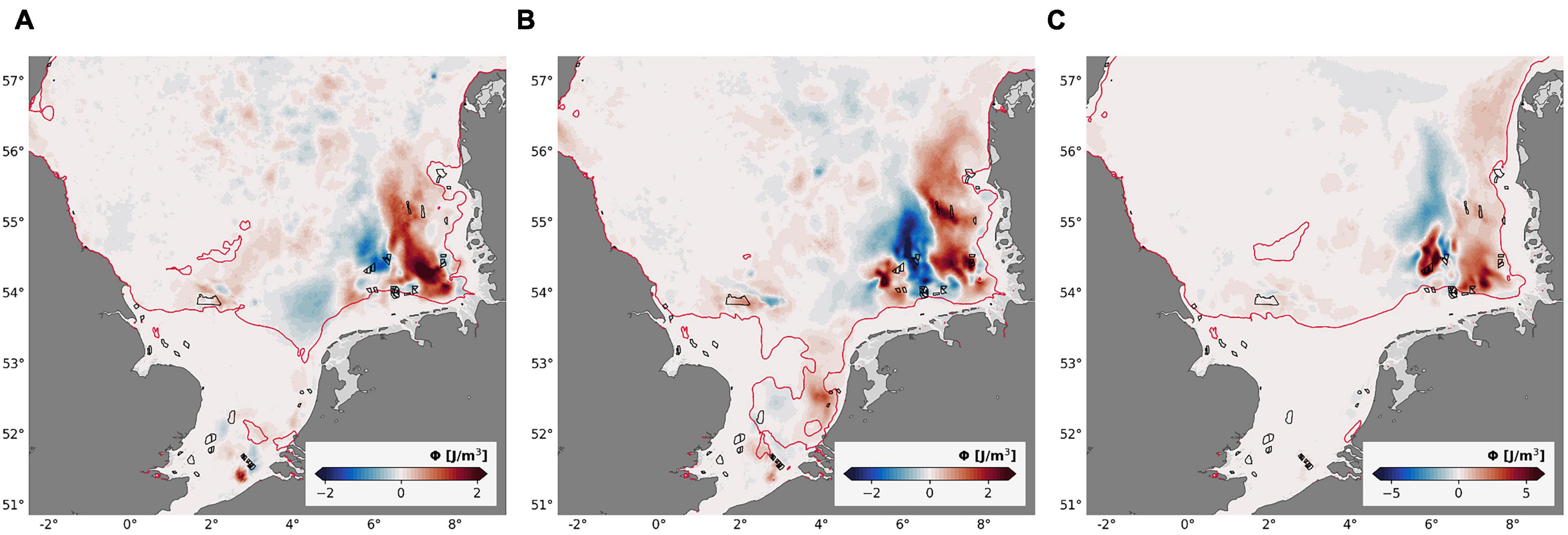
Figure 9. Monthly mean changes in stratification (potential energy anomaly Φ) for the months of June (A), July (B), and August (C). The red lines indicate the location of the mean tidal mixing fronts within the respective months. Black polygons indicate offshore wind farms.

The comparison of the monthly means shows a seasonal trend in the intensity of the impact on the potential energy anomaly (Figure 9). Initially, as the summer stratification evolves (Figures 9A,B), the patterns have a strong correlation to the spatial changes in the sea surface temperature and salinity (see Supplementary Figures A4, A5). At this, the changes in potential energy anomaly range on average around ± 2 Jm^–3. However, during the decline of stratification toward autumn (Figure 9C), strong magnitudes of beyond ± 6 Jm^–3 arise in the German Bight, which account for about 10–20% of the actual mean stratification strength (Figure 4A). Thereby, the strongest changes in the potential energy anomaly arise in the center of the surface elevation dipole and in regions of declining stratification toward the Frisian coast. While the alterations within the dipole are expected to result from the dipole-related processes, changes near the tidal mixing fronts are presumably associated to the reduction of wind stress and hence of the reduction of mixing in regions of declining stratification. As the mixing reduces, the wake effects sustain stratification in areas of wind speed reduction and thus lead to the amplification of stratification.

Figure 10 depicts the vertical profiles at wind farms, similar to Figures 6B–D, for the mean mixing rate K_v for the months of June to September. The vertical profiles support the assumption about the impact of the mixing alterations on the development of the summer stratification. As seen for the month of May (Figure 6B), the mixing at wind farms generally decreases in all months of the simulation as a result of the wind speed reduction. Thereby, the most pronounced changes occur around the mixed layer depth and in deep waters. In comparison of the different months, however, it is notable that the strongest reductions in mixing occur during the formation (May and June) and the breakdown (August and September) of the summer stratification. Especially toward autumn, the changes are up to five to ten times stronger than in the other months. At this, the maximum deficits generally occur near the mixed layer depth, which emphasizes the enhancement of stratification and the shallowing of the surface mixed layer at offshore wind farms due to atmospheric wake effects.

FIGURE 10

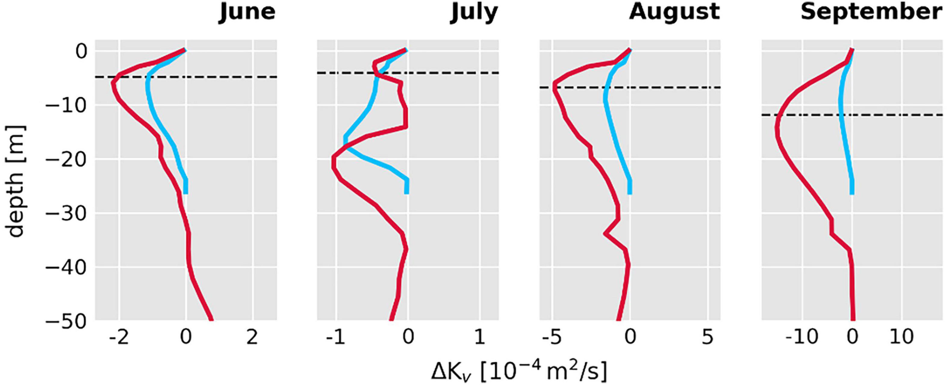
Figure 10. Monthly mean profiles in mixing rate for the period of June to September. The dashed lines indicate the location of the mixed layer depth. For the profiles, grid points within 5 km around each wind farm were considered. Profiles are divided into deep (z ≥ 25 m, red lines) and shallow (z < 25 m, blue lines) water depths.

Conclusion

As wind turbines extract kinetic energy from the wind field, atmospheric wakes result on the leeward side of offshore wind farms and affect the far field wind speed near the sea surface boundary. However, wind farm wakes and their impact on the hydrodynamic system represent a multivariate system, which is highly sensitive to external influences in atmosphere and ocean. In this study, we developed an empirical approach to describe the wake-related wind speed deficits in a hydrodynamic model. With this, we provided first insights about the interference of single wake effects due to the recent offshore wind energy production and resulting larger-scale disturbances in hydro- and thermodynamics in the southern and central North Sea. The implemented wake model generated wakes with constant dimensions, which, in terms of the different wind farm properties (e.g., the number of turbines and turbine density) or the changing atmospheric conditions, lead to over- and underestimation of the actual wake dimensions. Although the actual wake dimensions might vary in reality, the basic impact of wind farms, namely the downstream reduction in wind speed, is sufficiently considered to investigate the general consequences of wind speed deficits due to offshore wind farms. However, a more specific and realistic formulation will be important for more detailed future studies, since the wake dimensions determine the intensity of the associated impacts.

Over time, the extraction of energy by offshore wind farms results in extensive areas of reduced wind speed and subsequently the decrease of the shear-driven forcing at the sea surface boundary. As this reduces the momentum transfer from the atmosphere into the ocean, horizontal velocities and turbulent mixing initially decrease several tens of kilometers around offshore wind farms. Thereby the induced perturbations imply significant changes for the residual currents in the respective areas. Furthermore, convergence and divergence of water masses lead to the formation of sea surface elevation dipoles, which over time merge into large coherent structures. As shown here, these large-scale anomalies in the sea surface elevation are one of the main drivers of wake-related processes in the ocean. In addition to the general reduction of turbulent mixing, the large-scale sea level alterations trigger lateral and vertical changes in the temperature and salinity distribution and affect the hydrodynamics in areas covered by offshore wind farms. However, the magnitude of these changes is rather small compared to the long-term variability of temperature and salinity and can hardly be distinguished from the interannual variability. A severe overall impact by the wake effects on the ocean’s thermodynamic properties is thus not expected but rather large-scale structural change in the stratification strength and unanticipated mesoscale spatial variability in the mean current field. Nevertheless, further investigations are necessary to assess possible feedback on the air-sea exchange and thus potential impact on the regional atmospheric conditions, since surface heating along with the reduction in turbulent mixing influences the upward heat and momentum fluxes from the ocean into the atmosphere.

In this study, the structural changes in stratification become noticeable in a couple of ways. Firstly, we observed large dipole-related changes in the potential energy anomaly, as the geostrophic and baroclinic changes alter the temperature and salinity distribution. Secondly, the reduction of mixing at offshore wind farms results in the enhancement of the stratification strength, in particular, during the decline of the summer stratification. While the structural changes in stratification are minor in shallow mixed waters, the pronounced alterations in stratified waters can translate to the mixed layer depth, which likely increases or decreases depending on the respective stratification changes. This, in turn, might be crucial for marine ecosystem processes (Sverdrup, 1953). During the stratified summer months, the mixed layer depth is acting as barrier for nutrients and phytoplankton and plays a major role for the ecosystem dynamics. Therefore, induced fluctuations of the mixed layer depth can entail the intrusion of nutrients from the pycnocline into the surface mixed layer or the spreading of the nutrient-poor surface layer, respectively. The alterations in the nutrient availability, in turn, might affect local primary production and the nutrient balance. Thus, further studies are required to elucidate the impact on marine ecosystems and organisms in the North Sea, with regard to current and future wind farm scenarios.

Although the simulation was limited by the summer season of the year 2013, this study provides already important knowledge about the magnitude of implications of extensive offshore wind farming in the marine environment. Ultimately, the results showed that, in addition to the initial large-scale reduction in dynamics, wake effects cause internal processes, which affect the lateral and vertical transport of heat and salt even far beyond the associated wind farms. At this, changing wind directions inhibit severe local impact, as the varying internal processes mitigate each other. For the current state of wind energy production in the southern North Sea, the impact by the offshore wind farms entails structural changes in stratification strength and perturbations of the residual currents. Thereby, the cascading hydrodynamic processes particularly affect areas of clustered wind farms, like the German Bight. However, future wind energy development includes large installations in the Southern Bight and especially near the Dogger Bank, which will increase number of wind farms and hence possibly the impact in those areas (see Akhtar et al., 2021). Therefore, further investigations and improvements of the wake model are crucial, in order to assess the actual impact of future wind farm development in the North Sea environment. Especially since stratification anomalies entail perturbations of the pycnocline, assessment of potential biogeochemical impacts is of major interest.

Data Availability Statement

The original contributions presented in the study are included in the article/Supplementary Material, further inquiries can be directed to the corresponding author.

Author Contributions

NC generated the data set, performed the data analysis, and wrote the manuscript. BD performed statistical analysis and contributed to the parameterization section of the manuscript. UD and CS provided essential background knowledge and adviced to the study. CS initiated the idea of the study. All authors contributed to conception and design of the study, manuscript revision, read, and approved the submitted version.

Conflict of Interest

The authors declare that the research was conducted in the absence of any commercial or financial relationships that could be construed as a potential conflict of interest.

Publisher’s Note

All claims expressed in this article are solely those of the authors and do not necessarily represent those of their affiliated organizations, or those of the publisher, the editors and the reviewers. Any product that may be evaluated in this article, or claim that may be made by its manufacturer, is not guaranteed or endorsed by the publisher.

Acknowledgments

We would like to acknowledge the contribution by Johannes Schulz-Stellenfleth to the development of the wake parameterization. We would like to thank Jeffrey R. Carpenter and Thomas Pohlmann for helpful advice and appreciate the help by Johannes Pein regarding the SCHISM model. We appreciate the use of the mHM river discharge data generated by Rohini Kumar and Oldrich Rakovec and mapped onto the SCHISM grid by Stefan Hagemann. The data originate from a collaborative effort led by Sabine Attinger (Umweltforschungszentrum Leipzig) and Corinna Schrum (Helmholtz-Zentrum Hereon) that was supported by funding from the Initiative and Networking Fund of the Helmholtz Association through the project “Advanced Earth System Modelling Capacity (ESM).” This project is a contribution to theme “C3: Sustainable Adaption Scenarios for Coastal Systems” of the Cluster of Excellence EXC 2037 “CLICCS – Climate, Climatic Change, and Society” – Project Number: 390683824 funded by the Deutsche Forschungsgemeinschaft (DFG, German Research Foundation) under Germany‘s Excellence Strategy and to the CLICCS-HGF networking project funded by the Helmholtz-Gemeinschaft Deutscher Forschungszentren (HGF).

Supplementary Material

The Supplementary Material for this article can be found online at: https://www.frontiersin.org/articles/10.3389/fmars.2022.818501/full#supplementary-material

Footnotes

1. ^ https://www.esa.int/Applications/Observing_the_Earth/Copernicus/
2. ^ https://marine.copernicus.eu/
3. ^ http://www.ices.dk

References

Akhtar, N., Geyer, B., Rockel, B., Sommer, P. S., and Schrum, C. (2021). Accelerating deployment of offshore wind energy alter wind climate and reduce future power generation potentials. Sci. Rep. 11:11826. doi: 10.1038/s41598-021-91283-3

PubMed Abstract | CrossRef Full Text | Google Scholar

Broström, G. (2008). On the influence of large wind farms on the upper ocean circulation. J. Mar. Syst. 74, 585–591. doi: 10.1016/j.jmarsys.2008.05.001

CrossRef Full Text | Google Scholar

Cañadillas, B., Foreman, R., Barth, V., Siedersleben, S., Lampert, A., and Platis, A. (2020). Offshore wind farm wake recovery: Airborne measurements and its representation in engineering models. Wind Energy 23, 1249–1265. doi: 10.1002/we.2484

CrossRef Full Text | Google Scholar

Carpenter, J. R., Merckelbach, L., Callies, U., Clark, S., Gaslikova, L., and Baschek, B. (2016). Potential Impacts of Offshore Wind Farms on North Sea Stratification. PLoS One 11:e0160830. doi: 10.1371/journal.pone.0160830

PubMed Abstract | CrossRef Full Text | Google Scholar

Christiansen, M. B., and Hasager, C. B. (2005). Wake effects of large offshore wind farms identified from satellite SAR. Remote Sens. Env. 98, 251–268. doi: 10.1016/j.rse.2005.07.009

CrossRef Full Text | Google Scholar

Christiansen, M. B., and Hasager, C. B. (2006). Using airborne and satellite SAR for wake mapping offshore. Wind Energ. 9, 437–455. doi: 10.1002/we.196

CrossRef Full Text | Google Scholar

Cornes, R. C., van der Schrier, G., van den Besselaar, E. J. M., and Jones, P. D. (2018). An Ensemble Version of the E-OBS Temperature and Precipitation Data Sets. J. Geophys. Res. Atmos. 123, 9391–9409. doi: 10.1029/2017JD028200

CrossRef Full Text | Google Scholar

Daewel, U., and Schrum, C. (2013). Simulating long-term dynamics of the coupled North Sea and Baltic Sea ecosystem with ECOSMO II: Model description and validation. J. Mar. Syst. 119-120, 30–49. doi: 10.1016/j.jmarsys.2013.03.008

CrossRef Full Text | Google Scholar

Daewel, U., and Schrum, C. (2017). Low-frequency variability in North Sea and Baltic Sea identified through simulations with the 3-D coupled physical–biogeochemical model ECOSMO. Earth Syst. Dynam. 8, 801–815. doi: 10.5194/esd-8-801-2017

CrossRef Full Text | Google Scholar

Djath, B., and Schulz-Stellenfleth, J. (2019). Wind speed deficits downstream offshore wind parks? A new automised estimation technique based on satellite synthetic aperture radar data. Meteorologische Zeitschrift 28, 499–515. doi: 10.1127/metz/2019/0992

CrossRef Full Text | Google Scholar

Djath, B., Schulz-Stellenfleth, J., and Cañadillas, B. (2018). Impact of atmospheric stability on X-band and C-band synthetic aperture radar imagery of offshore windpark wakes. J. Renew. Sust. Energy 10:43301. doi: 10.1063/1.5020437

CrossRef Full Text | Google Scholar

Emeis, S. (2010). A simple analytical wind park model considering atmospheric stability. Wind Energ. 13, 459–469. doi: 10.1002/we.367

CrossRef Full Text | Google Scholar

Emeis, S., and Frandsen, S. (1993). Reduction of horizontal wind speed in a boundary layer with obstacles. Bound. Layer Meteorol. 64, 297–305. doi: 10.1007/BF00708968

CrossRef Full Text | Google Scholar

Emeis, S., Siedersleben, S., Lampert, A., Platis, A., Bange, J., and Djath, B. (2016). Exploring the wakes of large offshore wind farms. J. Phys. 753:92014. doi: 10.1088/1742-6596/753/9/092014

CrossRef Full Text | Google Scholar

Fitch, A. C., Lundquist, J. K., and Olson, J. B. (2013). Mesoscale Influences of Wind Farms throughout a Diurnal Cycle. Monthly Weather Rev. 141, 2173–2198. doi: 10.1175/MWR-D-12-00185.1

CrossRef Full Text | Google Scholar

Fitch, A. C., Olson, J. B., Lundquist, J. K., Dudhia, J., Gupta, A. K., and Michalakes, J. (2012). Local and Mesoscale Impacts of Wind Farms as Parameterized in a Mesoscale NWP Model. Monthly Weather Rev. 140, 3017–3038. doi: 10.1175/MWR-D-11-00352.1

CrossRef Full Text | Google Scholar

Frandsen, S. (1992). On the wind speed reduction in the center of large clusters of wind turbines. J. Wind Eng. Indust. Aerodynam. 39, 251–265. doi: 10.1016/0167-6105(92)90551-K

CrossRef Full Text | Google Scholar

Frandsen, S., Barthelmie, R., Pryor, S., Rathmann, O., Larsen, S., and Højstrup, J. (2006). Analytical modelling of wind speed deficit in large offshore wind farms. Wind Energ. 9, 39–53. doi: 10.1002/we.189

CrossRef Full Text | Google Scholar

Grashorn, S., and Stanev, E. V. (2016). Kármán vortex and turbulent wake generation by wind park piles. Ocean Dyn. 66, 1543–1557. doi: 10.1007/s10236-016-0995-2

CrossRef Full Text | Google Scholar

Hasager, C. B., Vincent, P., Badger, J., Badger, M., Di Bella, A., and Peña, A. (2015). Using Satellite SAR to Characterize the Wind Flow around Offshore Wind Farms. Energies 8, 5413–5439. doi: 10.3390/en8065413

CrossRef Full Text | Google Scholar

Hersbach, H., Stoffelen, A., and Haan, S. (2007). An improved C-band scatterometer ocean geophysical model function: CMOD5. J. Geophys. Res. 112:3743. doi: 10.1029/2006JC003743

CrossRef Full Text | Google Scholar

Holt, J., and Proctor, R. (2008). The seasonal circulation and volume transport on the northwest European continental shelf: A fine-resolution model study. J. Geophys. Res. 113:4034. doi: 10.1029/2006JC004034

CrossRef Full Text | Google Scholar

HZG (2017). coastDat-3_COSMO-CLM_ERAi. World Data Center for Climate (WDCC) at DKRZ. Available online at: http://cera-www.dkrz.de/WDCC/ui/Compact.jsp?acronym=coastDat-3_COSMO-CLM_ERAi (accessed date 2017-11-02)

Google Scholar

Jensen, N. O. (1983). A note on wind generator interaction. Roskilde: Risø National Laboratory.

Google Scholar

Kantha, L., and Clayson, C. A. (2015). “BOUNDARY LAYER (ATMOSPHERIC) AND AIR POLLUTION | Ocean Mixed Layer,” in Encyclopedia of Atmospheric Sciences (Second Edition), Vol. 2015, eds G. R. North, J. Pyle, and F. Zhang (Oxford: Academic Press), 290–298.

Google Scholar

Kumar, R., Samaniego, L., and Attinger, S. (2013). Implications of distributed hydrologic model parameterization on water fluxes at multiple scales and locations. Water Resour. Res. 49, 360–379. doi: 10.1029/2012WR012195

CrossRef Full Text | Google Scholar

Li, X., and Lehner, S. (2013). Observation of TerraSAR-X for Studies on Offshore Wind Turbine Wake in Near and Far Fields. IEEE J. Sel. Top. Appl. Earth Observ. Rem. Sens. 6, 1757–1768. doi: 10.1109/JSTARS.2013.2263577

CrossRef Full Text | Google Scholar

Lissaman, P. B. S. (1979). Energy Effectiveness of Arbitrary Arrays of Wind Turbines. J. Energy 3, 323–328. doi: 10.2514/3.62441

CrossRef Full Text | Google Scholar

Ludewig, E. (2015). On the Effect of Offshore Wind Farms on the Atmosphere and Ocean Dynamics. Cham: Springer International Publishing.

Google Scholar

Mathis, M., and Pohlmann, T. (2014). Projection of physical conditions in the North Sea for the 21st century. Clim. Res. 61, 1–17. doi: 10.3354/cr01232

CrossRef Full Text | Google Scholar

Otto, L., Zimmerman, J. T. F., Furnes, G. K., Mork, M., Saetre, R., and Becker, G. (1990). Review of the physical oceanography of the North Sea. Neth. J. Sea Res. 26, 161–238. doi: 10.1016/0077-7579(90)90091-T

CrossRef Full Text | Google Scholar

Paskyabi, M. B. (2015). “Offshore Wind Farm Wake Effect on Stratification and Coastal Upwelling,” in 12th Deep Sea Offshore Wind R&D Conference, EERA DeepWind’2015, Vol. 80, (Trondheim), 131–140. doi: 10.1016/j.egypro.2015.11.415

CrossRef Full Text | Google Scholar

Paskyabi, M. B., and Fer, I. (2012). “Upper Ocean Response to Large Wind Farm Effect in the Presence of Surface Gravity Waves,” in Selected papers from Deep Sea Offshore Wind R&D Conference, Vol. 24, (Trondheim), 245–254. doi: 10.1016/j.egypro.2012.06.106

CrossRef Full Text | Google Scholar

Peña, A., and Rathmann, O. (2014). Atmospheric stability-dependent infinite wind-farm models and the wake-decay coefficient. Wind Energ. 17, 1269–1285. doi: 10.1002/we.1632

CrossRef Full Text | Google Scholar

Platis, A., Bange, J., Bärfuss, K., Cañadillas, B., Hundhausen, M., and Djath, B. (2020). Long-range modifications of the wind field by offshore wind parks? Results of the project WIPAFF. Meteorologische Zeitschrift 29, 355–376. doi: 10.1127/metz/2020/1023

CrossRef Full Text | Google Scholar

Platis, A., Hundhausen, M., Mauz, M., Siedersleben, S., Lampert, A., and Bärfuss, K. (2021). Evaluation of a simple analytical model for offshore wind farm wake recovery by in situ data and Weather Research and Forecasting simulations. Wind Ener. 24, 212–228. doi: 10.1002/we.2568

CrossRef Full Text | Google Scholar

Platis, A., Siedersleben, S. K., Bange, J., Lampert, A., Bärfuss, K., and Hankers, R. (2018). First in situ evidence of wakes in the far field behind offshore wind farms. Sci. Rep. 8:2163. doi: 10.1038/s41598-018-20389-y

PubMed Abstract | CrossRef Full Text | Google Scholar

Samaniego, L., Kumar, R., and Attinger, S. (2010). Multiscale parameter regionalization of a grid-based hydrologic model at the mesoscale. Water Resour. Res. 46:7327. doi: 10.1029/2008WR007327

CrossRef Full Text | Google Scholar

Schrum, C. (2017). Regional Climate Modeling and Air-Sea Coupling. Oxford Res. Encyclop. Clim. Sci. 2017:3. doi: 10.1093/acrefore/9780190228620.013.3

CrossRef Full Text | Google Scholar

Schrum, C., and Backhaus, J. O. (1999). Sensitivity of atmosphere–ocean heat exchange and heat content in the North Sea and the Baltic Sea. Tellus A 51, 526–549. doi: 10.1034/j.1600-0870.1992.00006.x

PubMed Abstract | CrossRef Full Text | Google Scholar

Schrum, C., Lowe, J., Meier, H. E. M., Grabemann, I., Holt, J., and Mathis, M. (2016). “Projected Change - North Sea,” in North Sea Region Climate Change Assessment, eds M. Quante and F. Colijn (Cham: Springer International Publishing), 175–217.

Google Scholar

Schrum, C., Siegismund, F., and St. John, M. (2003). Decadal variations in the stratification and circulation patterns of the North Sea; are the 90’s unusual? ICES Mar. Sci. Symp. 219, 121–131.

Google Scholar

Schultze, L. K. P., Merckelbach, L. M., Horstmann, J., Raasch, S., and Carpenter, J. R. (2020). Increased Mixing and Turbulence in the Wake of Offshore Wind Farm Foundations. J. Geophys. Res. Oceans 125:e2019JC015858. doi: 10.1029/2019JC015858

CrossRef Full Text | Google Scholar

Shapiro, C. R., Starke, G. M., Meneveau, C., and Gayme, D. F. (2019). A Wake Modeling Paradigm for Wind Farm Design and Control. Energies 12:12152956. doi: 10.3390/en12152956

CrossRef Full Text | Google Scholar

Siedersleben, S. K., Platis, A., Lundquist, J. K., Lampert, A., Bärfuss, K., and Cañadillas, B. (2018). Evaluation of a Wind Farm Parametrization for Mesoscale Atmospheric Flow Models with Aircraft Measurements. Meteorologische Zeitschrift 27, 401–415. doi: 10.1127/metz/2018/0900

CrossRef Full Text | Google Scholar

Simpson, J. H., and Bowers, D. (1981). Models of stratification and frontal movement in shelf seas. Deep Sea Research Part A. Oceanogr. Res. Papers 28, 727–738. doi: 10.1016/0198-0149(81)90132-1

CrossRef Full Text | Google Scholar

Skogen, M. D., Drinkwater, K., Hjøllo, S. S., and Schrum, C. (2011). North Sea sensitivity to atmospheric forcing. J. Mar. Syst. 85, 106–114. doi: 10.1016/j.jmarsys.2010.12.008

CrossRef Full Text | Google Scholar

Sündermann, J., and Pohlmann, T. (2011). A brief analysis of North Sea physics. Oceanologia 53, 663–689. doi: 10.5697/oc.53-3.663

CrossRef Full Text | Google Scholar

Sverdrup, H. U. (1953). On Conditions for the Vernal Blooming of Phytoplankton. ICES J. Mar. Sci. 18, 287–295. doi: 10.1093/icesjms/18.3.287

CrossRef Full Text | Google Scholar

Taguchi, E., Stammer, D., and Zahel, W. (2014). Inferring deep ocean tidal energy dissipation from the global high-resolution data-assimilative HAMTIDE model. J. Geophys. Res. Oceans 119, 4573–4592. doi: 10.1002/2013JC009766

CrossRef Full Text | Google Scholar

Taylor, K. E. (2001). Summarizing multiple aspects of model performance in a single diagram. J. Geophys. Res. 106, 7183–7192. doi: 10.1029/2000JD900719

CrossRef Full Text | Google Scholar

Volker, P. J. H., Badger, J., Hahmann, A. N., and Ott, S. (2015). The Explicit Wake Parametrisation V1.0: a wind farm parametrisation in the mesoscale model WRF. Geosci. Mod. Dev. 8, 3715–3731. doi: 10.5194/gmd-8-3715-2015

CrossRef Full Text | Google Scholar

Zhang, Y. J., Ateljevich, E., Yu, H.-C., Wu, C. H., and Yu, J. C. (2015). A new vertical coordinate system for a 3D unstructured-grid model. Ocean Modelling 85, 16–31. doi: 10.1016/j.ocemod.2014.10.003

CrossRef Full Text | Google Scholar

Zhang, Y. J., Stanev, E. V., and Grashorn, S. (2016a). Unstructured-grid model for the North Sea and Baltic Sea: Validation against observations. Ocean Model. 97, 91–108. doi: 10.1016/j.ocemod.2015.11.009

CrossRef Full Text | Google Scholar

Zhang, Y. J., Ye, F., Stanev, E. V., and Grashorn, S. (2016b). Seamless cross-scale modeling with SCHISM. Ocean Model. 102, 64–81. doi: 10.1016/j.ocemod.2016.05.002

CrossRef Full Text | Google Scholar