Global-Scale Environmental Niche and Habitat of Blue Shark (Prionace glauca) by Size and Sex: A Pivotal Step to Improving Stock Management

Introduction

Rapid declines in the abundance of many elasmobranch populations in the last decades are largely attributed to vulnerability from exploitation (Dulvy et al., 2021). Elasmobranchs’ life history characteristics do not allow them to withstand elevated fishing mortalities for extended periods (Holden, 1974; Musick et al., 2000), and past accounts suggest that intensive fisheries can be followed by a rapid decline in catch rates or even a complete collapse of the fishery. In such a case, it has been documented that shark stocks may need several decades to recover (Castro et al., 1999). Shark declines can have strong ecological consequences. Except in coral reef ecosystems (Desbiens et al., 2021), the absence of sharks can indirectly alter predation pressure on different fish species via behavioral responses of meso-consumers released from predator intimidation (Frid et al., 2008), altering the total fish assemblage through trophic interactions and shaping marine communities over large spatial and temporal scales (Stevens et al., 2000; Ferretti et al., 2010). The manner in which sharks structure communities may also be shifting with climate change, where the recent increase of seawater temperatures has been linked to a poleward shift in shark distributions (Dolgov et al., 2005; Tanaka et al., 2021) and a potential reduction of dive depths due to increased deoxygenation (Vedor et al., 2021b).

The blue shark, Prionace glauca, is among the most abundant, widespread, fecund and fast-growing of elasmobranchs, making it somewhat more resilient to exploitation than other shark species (Castro et al., 1999; Aires-da-Silva and Gallucci, 2007). It is also one of the most heavily fished sharks in the world; annual fishing mortality (mainly as bycatch) is estimated at 10.74 million.year⁻¹ (95% PI, 4.64–15.76 million.year⁻¹; Clarke et al., 2006), representing 5% of global shark landings in the 1990s, peaking at almost 18% (137,973 mt) in 2013 before declining to 16% in 2017 (103,528 mt) (Okes and Sant, 2019).

As a bycatch species, the catch of blue sharks is intrinsically linked to abundance but also to global market demand, both being relatively complex drivers. Blue shark is amongst the most abundant shark species in international trade (Okes and Sant, 2019) for the meat and/or fins (e.g., dominant shark species for meat in Japan, Spain, Taiwan, and Uruguay: Okes and Sant, 2019; Brazil: Cruz et al., 2021; Italy: Serena and Silvestri, 2018; Mancusi et al., 2020). Overall, the importance of blue shark in the fin trade highlights its economic importance and the driver of the demand (Porcher et al., 2021). Although some fleets release blue shark bycatch (Campana, 2016), this species is a major component of retained incidental catch of longline and driftnet fisheries, particularly from nations with high-seas fleets (Okes and Sant, 2019), often seasonally complementing the catches of other pelagic species. For example, the blue shark is frequently the dominant bycatch species in swordfish and tuna longlining (Megalofonou et al., 2000; Campana et al., 2016; Carpentieri et al., 2021). Global spatial analyses reported blue shark to be at significantly greater risk of exposure to fishing due to its high distributional overlap with important fished areas (Queiroz et al., 2019). However blue shark populations have declined at the global scale less than other shark species in the last five decades (Pacoureau et al., 2021) probably due to its relatively higher reproductive and growth rates compared to other oceanic sharks (Pacoureau et al., 2021) and even though fishing mortality was close to or possibly exceeding the maximum sustainable yield levels (Clarke et al., 2006). Tuna Regional Fisheries Management Organizations (RFMOs) conduct several shark stock, but often no consensus on current status is found (e.g., ICCAT, 2015). If several shark-specific regulations exist (Simpfendorfer and Dulvy, 2017), one RFMO only recently started to agree on catch limits for blue shark (e.g., allocated total allowable catches (TAC) in the North Atlantic and unallocated TAC in the South Atlantic by ICCAT in 2019, (European Union, 2020; European Union, 2021).

Highly mobile in nature, blue sharks are known to make seasonal reproductive migrations following changes in water temperature and currents (Nakano, 1994; Stevens, 1999). The links between blue shark distribution and oceanographic features are an important focal point of current research. An improved knowledge of blue shark habitat is needed to better understand the ecology of a species that is distributed globally, but for which only regional patterns have been studied in detail (e.g., Bigelow et al., 1999; Carvalho et al., 2011; Adams et al., 2016; Vandeperre et al., 2016). The provision of robust regional patterns of size- or sex-specific habitat could improve the management of blue shark populations by providing relevant spatio-temporal information for potential fisheries mitigation measures. Focus should be given to the life history stages that are most vulnerable to fishing to possibly reduce the overall impact of its catch in global fisheries as target and bycatch species.

In this study, we investigate the relationship between global blue shark distribution and selected environmental variables to define the species environmental niche. We frame our results in the context of sustainable exploitation and conservation of this species, to provide new perspectives for research and management of blue shark populations. We justify the use of two environmental proxies for food availability (chlorophyll-a gradient and upper mesopelagic micronekton) as indicators of preferred sex- and size-specific foraging habitat and identify the unfavorable physical variables limiting habitat use. We then build a habitat model for each sex and size classes using these recognized environmental variables and clustering-based parametrizations. The predicted habitat distribution is compared with published knowledge, and model performance is quantitatively compared against an independent validation dataset of blue shark presence. The Supplementary Material provides substantial details for a deeper insight of the analysis and notably seven regional habitat animations by size and sex classes with the overlay of blue shark presence data (observer and electronic tagging data) for interpreting the seasonal movements.

Materials and Methods

Blue Shark Presence Data

We collected extensive blue shark presence data throughout its global distribution, mostly from observer programs of longline fisheries but also purse seine fisheries, and from electronic tagging programs. We used presence-only data from all collected datasets for consistency. The full dataset included 589,450 observations, but only 496,080 observations overlapped with the availability of environmental data (chlorophyll-a data from MODIS-Aqua satellite sensor and the other variables extracted from the EU-Copernicus Marine Environment Monitoring Service, respectively). Thus, we restricted all data to the time period from July 2002 to December 2018. This included fishery-independent 234 tracks from electronically tagged blue sharks in the Pacific (95), Atlantic (132), and Indian Oceans (7) using different types of electronic tags (Argos satellite transmitters and pop-up satellite-linked archival transmitters, PSATs) on which we applied filtering criteria for geolocation (see Supplementary Material, hereafter SM). For electronic tags that did not have precise location information (i.e., light- and temperature-based PSATs tags), the majority of the likelihood surface for position estimates tended to fall within a 50 km radius. This level of precision was considered to be similar to the longline data since we assumed sets had a maximum length of 100 km and we kept the midpoint as the geographic position. Redundancy of all presence data was avoided by filtering out data of the same size (and sex for large individuals) when closer than 2.3 km on the same day. This distance represented about half of the pixel size of the habitat model grid, which was determined by the resolution of the satellite remote sensing data of chlorophyll-a (1/24° by 1/24° resolution). However, this redundancy filter mostly removed eventual duplicates in the observer data since several longline sets generally do not occur in the same location and day. It was ineffective for electronic tagging data since only one high-precision location was kept per day (see SM).

The presence data were partitioned by size and sex classes following information available in the literature. While there are differences in size thresholds among ocean regions, we followed Vandeperre et al. (2016) and Megalofonou et al. (2009) for small and large juveniles, and we averaged values from the following sources: Castro and Mejuto (1995); Castro et al. (1999); Campana et al. (2006); Megalofonou et al. (2009); Calich and Campana (2015); Coelho et al. (2018) for adults of both sexes. From the 496,907 observations of blue shark presence between July 2002 to December 2018, the total number of observations with morphometric data (small juveniles with size information, larger blue sharks with size and sex and high-position quality for electronic tags) was 265,595 (see SM, Table SM.1). The small juvenile class was not split by sex as they tend to mix in temperate and subarctic waters (Nakano, 1994). The size classes considered were 1) small juveniles of both sexes (hereafter SJ) with fork length (FL) below 125 cm (n = 60,904 observations, 23%), 2) large juvenile females (hereafter LJF) with FL from 125 to 180 cm (n = 54,611, 21%), 3) large juvenile males (hereafter LJM) with FL from 125 to 190 cm (n = 90,792, 34%), 4) adult females (hereafter AF) with FL above 180 cm (n = 29,773, 11%) and adult males (hereafter AM) with FL above 190 cm (n = 29,515, 11%). Any presence information that was collected after the model calibration process or for which the environmental information was missing (e.g., missing satellite-derived chlorophyll-a) was used for validation only of the habitat model (see Model Performance section). After filtering (one high-precision location per day), the electronic tagging data accounted for 14,559 fishery-independent observations (906 for SJ, 4,160 for LJF, 2,355 for LJM, 2,350 for AF, and 4,788 for AM), representing 5.5% of the analyzed data. The overall data distribution by size and sex classes were: 22.9% for SJ, 20.6% for LJF, 34.2% for LJM, 11.2% for AF and 11.1% for AM. Figure 1 shows the spatial and seasonal distributions of the analyzed data (see SM for density maps by size and sex classes). Although the South-East Atlantic, the North and East of the Indian Ocean, and the Northwest Pacific are not well-represented in our dataset, the data spans a wide range of latitudes and productive ecosystems in the other areas, and likely accounts for most of the environmental variability of blue shark habitat.

FIGURE 1

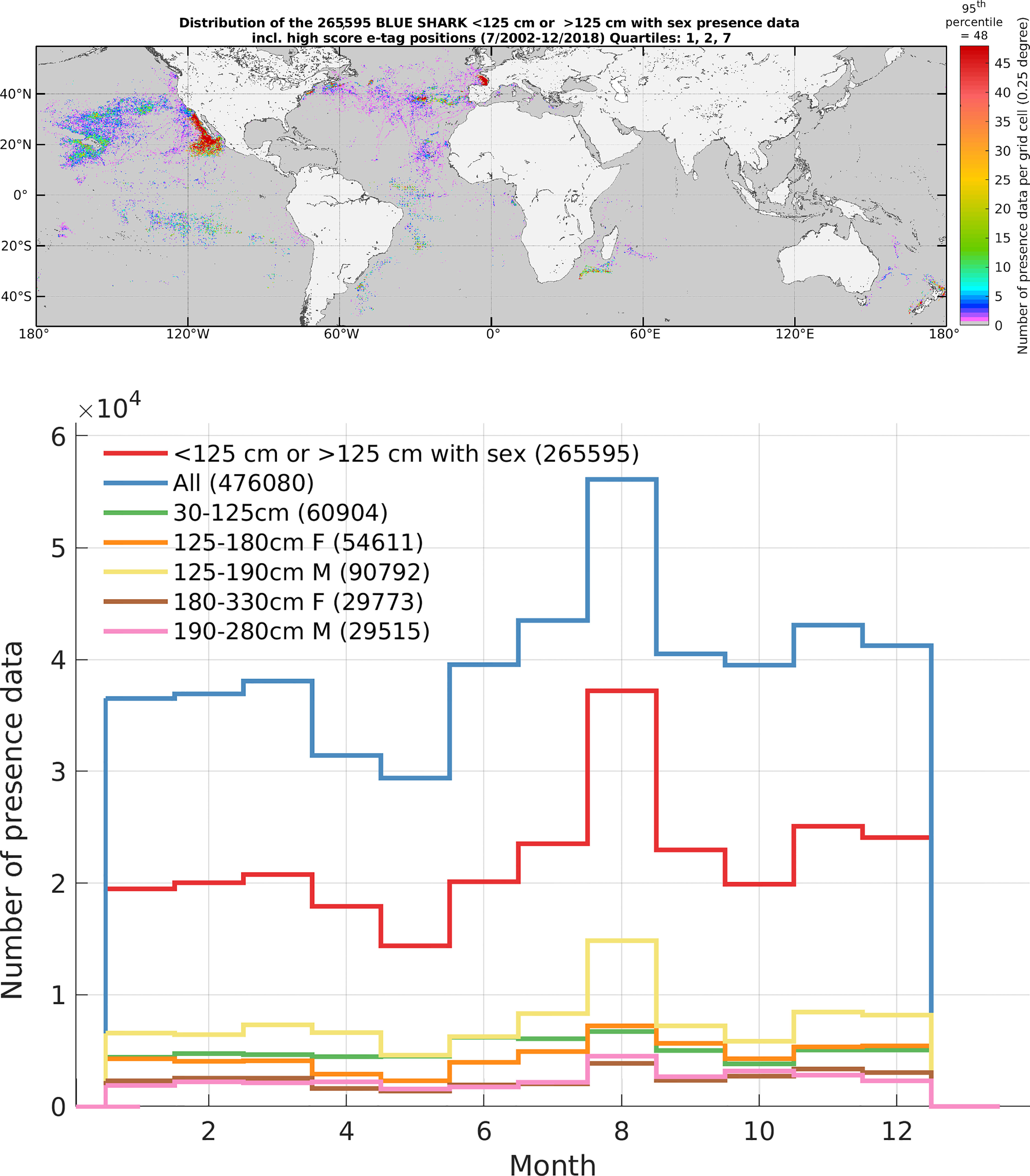
Figure 1 Distribution of both calibration and validation presence data (FL < 125 cm and FL > 125 cm with sex information, upper map, n = 265,595, number of presence data per grid cell of 0.25°), and monthly distribution by size and sex class (‘All’ corresponds to all presence data contemporary to environmental data independently of size and sex availability). These data are mainly derived from fisheries observer (94.5%) programs, but include a small amount of data from electronic tags (one position per day of higher accuracy, 5.5%). See in Supplementary Material the Figures SM.1-5 on the distributions by size and sex classes, and seven video animations of habitat in regions of high-density electronic tagging data.

From Ecological Traits to Modeling Foraging Habitat

The selection of environmental variables for modeling was guided by their relevance to reflect the main ecological traits of the blue shark. These choices were therefore based on past habitat analysis and expert knowledge as described in the following three sections. This species is known to have a wide distribution from equatorial to temperate latitudes (Vandeperre et al., 2014a; Coelho et al., 2018; Maxwell et al., 2019), inhabiting contrasting environments in terms of productivity. Similar to other large marine predators, the blue shark is attracted by mesoscale features such as fronts or eddies (Queiroz et al., 2012; Vandeperre et al., 2014b; Scales et al., 2018; Braun et al., 2019) in relatively plankton-rich surface waters (epipelagic and mesotrophic areas: defined hereafter as the depth layer from 0 to 1.5-times the euphotic depth with surface chlorophyll content in the range of 0.1-4.0 mg.m^-3). However, blue shark also makes use of relatively poor surface waters (oligotrophic, with surface chlorophyll content below about 0.1 mg.m^-3) and feeds in the upper mesopelagic layer (depth layer from 1.5 to 4.5-times the euphotic depth; e.g., Vedor et al., 2021a), with cephalopods as dominant prey (Cordova-Zavaleta et al., 2018; Konan et al., 2018). To reflect these contrasting environments, we retained surface chlorophyll-a fronts and mesopelagic micronekton as proxies for foraging behavior. Additionally, blue shark diving profiles suggest that behavioral thermoregulation has an important effect on hunting tactics (Campana et al., 2011; Braun et al., 2019). The blue shark diving profiles often show higher contrasts in temperature levels between the mesopelagic and the surface layer in tropical areas than when swimming within the intermediate layer in temperate latitudes. The primary function of these dives may be to follow the diurnal vertical migration of prey, with deeper dives during the day or during a full moon at night (Vedor et al., 2021a), but can also potentially be related to orientation (Campana et al., 2011; Musyl et al., 2011; Elliott, 2020). Similarly, blue sharks were shown to remain for longer durations at depth in the warmer anticyclonic eddies than in the cooler cyclonic eddies (Braun et al., 2019) or in the warmer Gulf Stream than in contiguous waters of the Labrador Current (Campana et al., 2011). Both of these behaviors would release the species from thermal constraints while foraging. Sea surface height anomaly (SSHa) is mainly influenced by seasonal changes in temperature and the geostrophic currents that characterize eddies and gyres that are known to shape the vertical and horizontal distribution of the full pelagic food web (Polovina et al., 2001; Tew Kai and Marsac, 2010; Godø et al., 2012), including the blue shark (Vandeperre et al., 2014b). Thus, water temperature within the mesotrophic or oligotrophic environments (sea surface temperature, SST, and the temperature 100 m below the mixed layer depth, T_mld+100), as well as sea surface height anomaly in regards to the mesoscale activity, would be expected to play a key role in the global distribution of blue sharks and were selected as highly discriminant variables in the present habitat modeling. Besides the abiotic environmental covariates retained for habitat modeling (SST, T_mld+100 and SSHa), global fields of biotic (chlorophyll-a fronts, mesopelagic micronekton) were included, as they could substantially help define the foraging habitat of the species. All environmental variables were extracted as mean values over a 25 km radius centered on the calibration presence data as this distance is relevant to most location uncertainty of blue shark observer and electronic tagging data, and is at the scale or below of oceanic features of importance (e.g., fronts or eddies) (see also Figure SM.6 for data integration). We particularly accounted for the ecological traits of the species and literature knowledge that highlighted some under-sampling of extreme environments in our presence dataset.

The Biotic Environmental Variables

The main proxies used for blue shark foraging in our model are the chlorophyll-a-derived productivity fronts in the mesotrophic areas and the mesopelagic micronekton in oligotrophic areas. Incorporating both of these is justified by i) the increased occupancy of blue shark in surface layers (upper 100 m) driven by highly productive (and cold) waters, and in deeper layers in oligotrophic (and warm) environments (Vedor et al., 2021a; Fujinami et al., 2021), ii) the efficient detection of mesoscale productivity features by satellite observation in relatively productive areas, and iii) the prediction of potential prey sources at depth (mesopelagic micronekton) in relatively poor-production environments where satellite observation is unsuitable. The lack of detection by satellite ocean color sensors of maximum chlorophyll-a in the subsurface oligotrophic environments due to light attenuation (exponential decrease of light with increasing depth) underestimates productivity in these oligotrophic environments. Therefore, we considered the best performance of both biotic variables between the high dynamics of productivity fronts, of importance for large pelagic predators and sensed by satellite observation, in mesotrophic waters and the deeper and lower dynamics of the simulated mesopelagic micronekton in oligotrophic environments.

In mesotrophic areas, the daily detection of productive oceanic features (chlorophyll-a fronts) from ocean color satellite sensors (currently MODIS-Aqua) is a good generic proxy for food availability to fish populations (Druon et al., 2021). When productivity fronts are active long enough (from weeks to months) to allow the development of mesozooplankton populations (Druon et al., 2019), they were shown to attract epi- and mesopelagic fish and top predators (Olson et al., 1994; Polovina et al., 2001; Briscoe et al., 2017; Druon et al., 2017; Baudena et al., 2021). After an initial development phase of 3-4 weeks, the mesozooplankton biomass reached substantial levels in the persistent and not necessarily stationary chlorophyll-a fronts, i.e. where chlorophyll-a gradient is high (Druon et al., 2019). This biomass aggregation may represent concomitant foraging hotspots for small pelagic fish, and result in active aggregation of highly mobile predators (e.g., bluefin tuna Thunnus thynnus in Druon et al., 2016; fin whale Balaenoptera physalus in Panigada et al., 2017, basking shark Cetorhinus maximus in Miller et al., 2015). Similarly, blue sharks have been shown to be attracted by frontal oceanic features (Bigelow et al., 1999). Daily chlorophyll-a (CHL, mg.m⁻³) data were gathered from the MODIS-Aqua ocean color sensor (years 2002–2018; 1/24° resolution) using the Ocean Color Index (OCI) algorithm (Hu et al., 2012) and extracted from the NASA portal (https://oceancolor.gsfc.nasa.gov/l3/; reprocessed January 2018). Small and large chlorophyll-a fronts were derived from and refer to different levels of chlorophyll-a gradient values (see the SM for details on the chlorophyll-a gradient calculation). Based on the link described above between productivity fronts and biomass of low and high trophic levels (e.g., Olson et al., 1994; Polovina et al., 2001; Druon et al., 2019; Druon et al., 2021; Baudena et al., 2021), high chlorophyll-a gradient levels are assumed to correspond, when persistent, to productivity fronts with an important capacity to sustain well-developed food chains and foraging opportunities for predators. The five-day chlorophyll-a gradient values were extracted in a 25 km radius centered on the (day and location of) blue shark presence data for each size and sex class, and a minimum of 33% coverage was set to accept the mean gradient value (5-day and 25 km-radius mean value). The histogram of extracted log-transformed gradient values was used to derive a dependent linear predictor, which is the main component of the daily foraging habitat in the mesotrophic environment.

In oligotrophic environments, the estimate of mesopelagic micronekton (‘micronekton upper mesopelagic & micronekton migrant upper mesopelagic’, in wet weight g.m^-2) was extracted from the global ocean low and mid trophic levels biomass content hindcast model, available through the EU-Copernicus Marine Environment Monitoring Service (https://marine.copernicus.eu/access-data). These variables are simulated by the SEAPODYM-LMTL (SEAPODYM for Low and Mid-Trophic Level organisms) model (Lehodey et al., 2015, see SI for details). Weekly data were aggregated by month and linearly interpolated from the original grid at 1/12° resolution to the habitat grid at 1/24° resolution.

For foraging proxies in the habitat model, we thus used the mesopelagic micronekton in oligotrophic areas (CHL < CHL_min) and productivity fronts in mesotrophic areas (CHL > CHL_min), noting that CHL_min was a relatively low chlorophyll-a value used as a threshold between both foraging proxies. The specific value of CHL_min for each blue shark class was identified using cluster analysis (the k-means clustering technique; see SM for full description).

The Abiotic Environmental Variables

The abiotic variables included in the habitat model were sea surface temperature (SST), sea surface height anomaly (SSHa), and the temperature 100 m below the mixed layer depth (T_mld+100). The variables that were not included in the habitat model were sea surface salinity, sea surface current intensity, surface oxygen content, and the depth of the mixed layer since they presented large variabilities (see SM) and were not identified as primary discriminant variables by the expert knowledge. A range of favorable conditions for each abiotic variable was defined and subsequently used to exclude unsuitable habitats. The 0.3^th and 99.7^th percentile values were selected for the favorable range of SST and SSHa for each size and sex class. This range was large enough to encompass some extreme environmental conditions that were poorly represented in the presence data, and included areas with contrasting SSTs yet high seasonal blue shark presence (e.g., in the Northwest Atlantic; see Results). More generally, we considered the expert knowledge (e.g., known presence in local extreme conditions) in the choice of these threshold values since the dataset likely over-represents some environments and under-represents others. The majority of blue shark observations came from fishery-dependent data, which are known to be spatially and temporally biased (Saul et al., 2020). We also excluded an intermediate range of SST for the blue shark female classes (LJF and AF) using the cluster analysis, noting a substantially low presence in this range (90^th and 10^th percentile values of two different clusters, see Results). Unlike the other abiotic exclusions, this intermediate SST levels within the favorable range for large females appeared to be actively avoided rather than corresponding to physical intolerance. Finally, our analyses showed that the temperature 100 m below the mixed layer depth (T_mld+100) was a relevant variable for identifying the upper limit of the mesopelagic layer. Micronekton was extracted from the mesopelagic layer, representing depths of 138 ± 32 m. This upper depth of the mesopelagic layer corresponds to a vertical position where large blue sharks spend a large proportion of the night, while deeper dives during the day are alternatively done with shallower dives in response to thermoregulation needs (Campana et al., 2011; Braun et al., 2019). Consequently, T_mld+100 was considered to represent an averaged-dive temperature, i.e. identifying the appropriate mean temperature representing a dive at the approximate interface between the epipelagic and upper mesopelagic layers. We selected the same minimum temperature value for T_mld+100 as for SST since the minimum levels of SST and T_mld+100 were considered to be the surface and mean-dive extreme temperature tolerance for each size and sex class. The fields of temperature, mixed layer depth, and sea surface height anomalies were extracted from the EU-Copernicus Marine Environment Monitoring Service global model (https://marine.copernicus.eu/access-data). All abiotic data were first linearly interpolated from the original grid at 1/12° resolution to the habitat grid at 1/24° resolution, and then linearly interpolated from monthly to daily values for estimating the daily habitat (see also Figure SM.6 for data integration).

The Blue Shark Environmental Envelope

The environmental envelope of a species is defined as the set of environments within which it is believed that are necessary to maintain viable populations (Walker and Cocks, 1991). All biotic and abiotic variables were integrated (mean value) over a 25 km radius centered on each presence data for the identification of the environmental envelope. This radius was selected as representative of the geolocation precision of most of the presence data (below about 50 km). Blue sharks of any size can easily cover this distance within a day, as the lower and upper bounds of the 95% confidence interval for the mean movement rate of large blue sharks was 34 ± 9 km.day^-1 and 52 ± 18 km.day^-1 (1.42 ± 0.38 km.h^-1 and 2.15 ± 0.73 km.h^-1, Kai and Fujinami, 2020). The habitat model for blue sharks evaluates positive relationships with foraging proxies (productivity fronts or mesopelagic micronekton) after unsuitable abiotic environments are excluded (based on SST, T_mld+100 and SSHa). The resulting modeling envelope has two main components depending on the level of surface chlorophyll-a: the oligotrophic (CHL < CHL_min) and mesotrophic (CHL_min < CHL < CHL_max) foraging habitats that use mesopelagic micronekton and productivity fronts (chlorophyll-a horizontal gradients), respectively (Figure 2). Both components were associated with the abiotic variables, i.e., temperature and SSHa, where a value of 1 was set for favorable levels and a value of 0 otherwise, therefore excluding unfavorable levels from the habitat. As described above, a minimum temperature value in the upper mesopelagic layer (T_mld+100) was used to exclude waters in oligotrophic environments that were too cold for diving blue sharks, while a suitable range of SST was used to exclude unsuitably warm or cold waters from the habitat in mesotrophic waters. When a specific size class avoided certain sea surface temperatures (large females, LJF and AF), the associated daily foraging habitat in this intermediate SST range was set to 0.

FIGURE 2

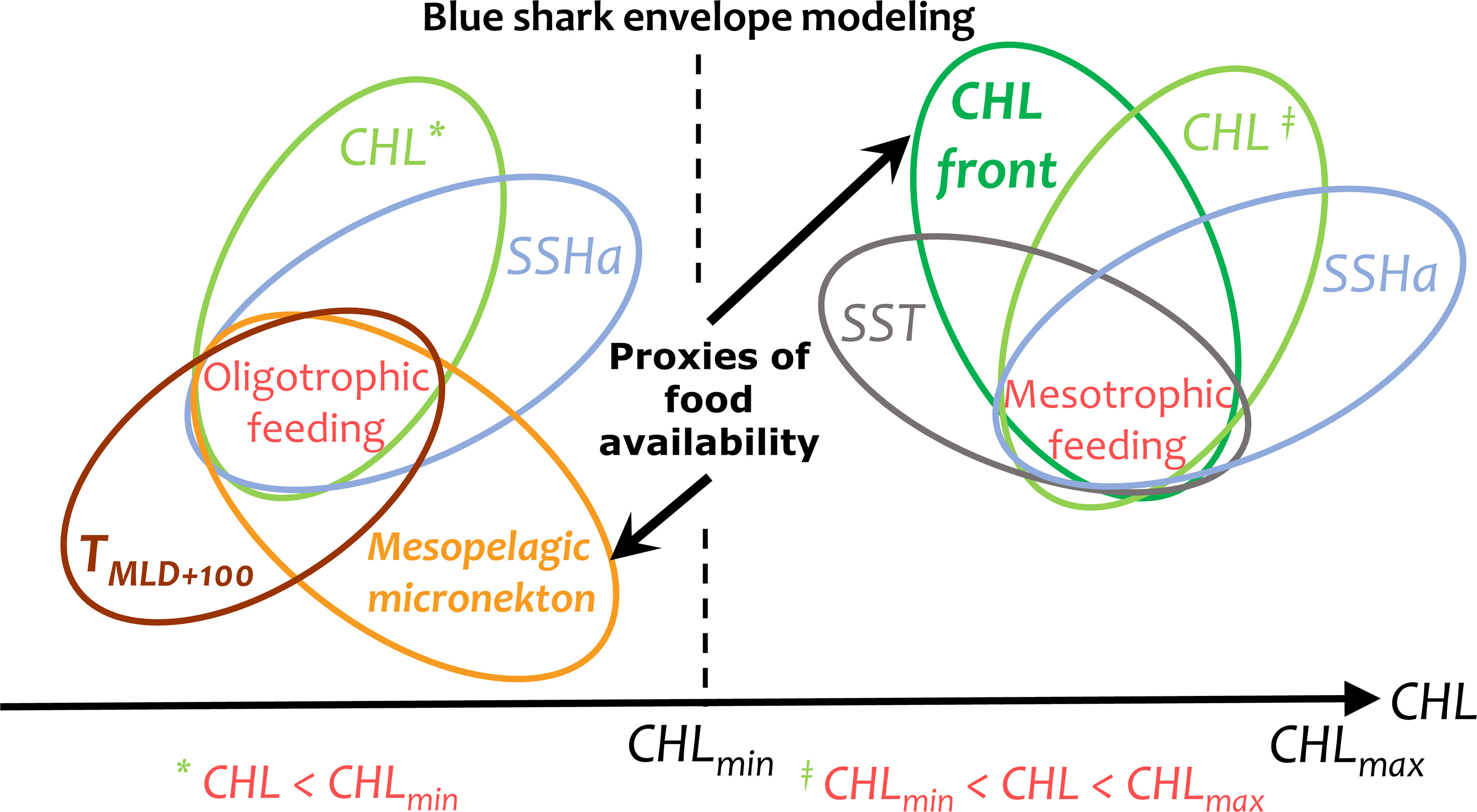
Figure 2 Scheme of the blue shark envelope modeling linking the environmental variables in oligotrophic (CHL < CHL_min) and mesotrophic (CHL_min < CHL < CHL_max) environments with mesopelagic micronekton and productivity fronts (chlorophyll-a horizontal gradients) as foraging proxies, respectively. The abiotic variables (SST, T_mld+100 and SSHa) were used to exclude unsuitable environments. CHL, surface chlorophyll-a content; SST, sea surface temperature; T_mld+100, Temperature 100 m below the mixed layer depth; SSHa, sea surface height anomaly.

The same calibration method that was used to estimate the quality of foraging habitat (i.e., prediction of foraging opportunities) was applied to mesopelagic micronekton and productivity fronts (MMnekton and gradCHL, respectively). The habitat model for both these foraging proxies has two parameters besides the distinct CHL range on which they apply (CHL < CHL_min for mesopelagic micronekton and CHL_min < CHL < CHL_max for productivity fronts): a minimum and intermediate value of mesopelagic micronekton (MMnekton) and a horizontal gradient of chlorophyll-a (gradCHL, Table 1). The minimum and intermediate threshold values for MMnekton define the slope of daily habitat quality in the oligotrophic environments (and similarly for gradCHL in the mesotrophic environments). The intermediate threshold value (the upper part of the habitat slope) is the minimum value of MMnekton or gradCHL that corresponds to a habitat index of 1. The suitable CHL range and the minimum threshold of foraging proxies (MMnekton_min and gradCHL_min) were identified using cluster analysis (see SM for details on the clustering) and represent the boundary values of suitable foraging environments for each size and sex class. The intermediate value of each proxy (MMnekton_int and gradCHL_int), which define minimum levels of MMnekton and gradCHL corresponding to the maximum daily habitat of 1, was identified using the values of MMnekton_min and gradCHL_min and the preferred range of MMnekton and gradCHL. This preferred range of each foraging proxy was defined by the maximum slope of the cumulative distribution that corresponds to presence data in the respective CHL range (CHL < CHL_min for MMnekton and CHL_min < CHL < CHL_max for gradCHL). A break in the daily habitat index between 0 and 0.3 was inserted to reflect sub-optimal foraging opportunities (i.e., no effective foraging). However, such areas are still important for a highly mobile predator to detect prey gradients and actively move towards higher densities. Overall, there is no direct correspondence between the daily foraging habitat function for both foraging proxies (MMnekton and gradCHL), even though each proxy quantitatively reflects the level of foraging opportunities (see Discussion).

TABLE 1

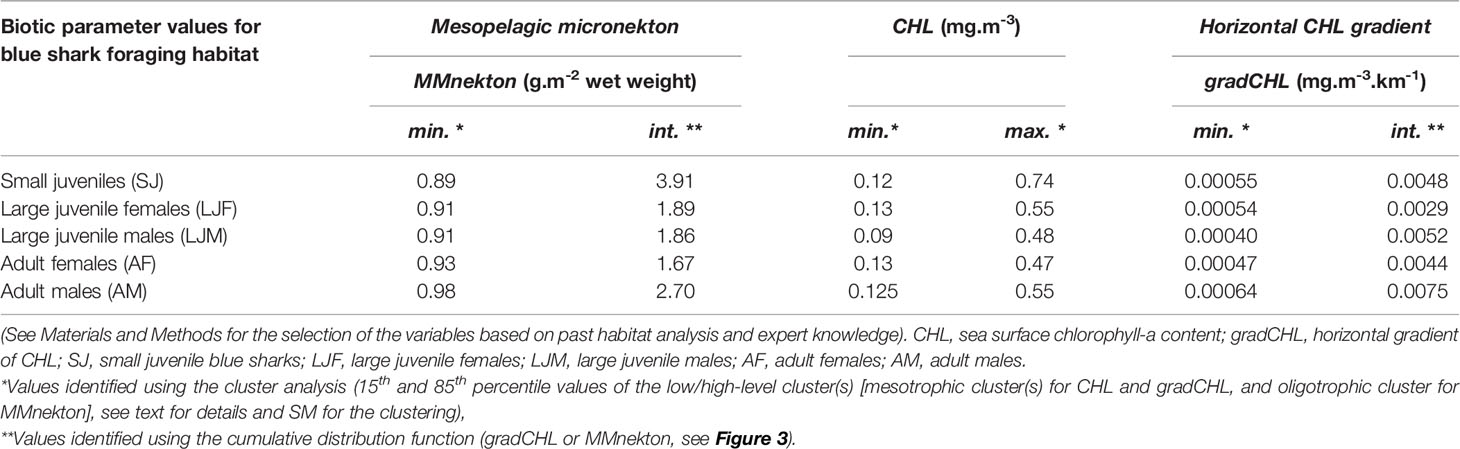
Table 1 Calibration parameters for the biotic variables of the blue shark foraging habitat model.

Habitat Index Equations by Size and Sex Classes

Increasing levels within each foraging proxy, from small to large productivity fronts or from low to high mesopelagic micronekton levels were standardized from 0 to 1 in the daily productive habitat indices. Daily foraging habitat was then filtered by the various abiotic limitations, scored as 1 (inside the favorable range) or 0 (outside). Thus, daily foraging habitat was defined in each grid cell as satisfying the following equations for suitable environmental conditions:

$$\begin{array}{l}FeedingHabita{t}_{Day,Cell}\\ =\{\begin{array}{l}0if\left(CHL<CH{L}_{min}\text{ and }MMnekton<MMnekto{n}_{min}\right)or\\ \left(CH{L}_{min}<CHL<CH{L}_{max}\text{ and }gradCHL<gradCH{L}_{min}\right)or\\ CHL>CH{L}_{max}\\ \begin{array}{l}0to1if\ast \left(CHL<CH{L}_{min}MMnekto{n}_{min}<MMnekton<MMnekto{n}_{int}\right)or\\ \ast \ast \left(CH{L}_{min}<CHL<CH{L}_{max}\text{ and }gradCH{L}_{min}<gradCHL<gradCH{L}_{int}\right)\end{array}\\ \begin{array}{l}1if\left(CHL<CH{L}_{min}\text{ and }MMnekton>MMnekto{n}_{int}\right)or\\ \left(CH{L}_{\min }<CHL<CH{L}_{max}\text{ and }gradCHL>gradCH{L}_{int}\right)\end{array}\end{array}\end{array}$$

*linear function from 0 to 1 as follows:

$$ForagingHabita{t}_{Day,Cell}=1+\frac{MMnekton-MMnekto{n}_{int}}{MMnekto{n}_{int}-MMnekto{n}_{min}}$$

**linear function from 0 to 1 as follows:

$$ForagingHabita{t}_{Day,Cell}=1+\frac{ln\left(gradCHL\right)-ln\left(gradCH{L}_{int}\right)}{ln\left(gradCH{L}_{int}\right)-ln\left(gradCH{L}_{min}\right)}$$

where ln is the natural logarithm, CHL_min and CHL_max define the suitable range of chlorophyll-a, and MMnekton_min and MMnekton_int are the minima and intermediate thresholds of the mesopelagic micronekton concentration. The latter two thresholds bound the increasing linear function for each suitable habitat index between 0 and 1 (the same reasoning applies to the gradCHL linear function).

The areas that met the daily biotic and abiotic requirements of the habitat model were then integrated over time to create monthly foraging habitat suitability maps. The time composites are expressed in frequency of suitable habitat occurrence (%) computed as a mean of 0-to-1 daily values quantitatively associated with either the respective foraging proxy. The multi-annual composites showing seasonal patterns were computed from the monthly means to set an equal weight between months. This is particularly relevant since lower habitat coverage occurs during winter due to the higher cloud presence and the subsequent greater number of missing estimates of satellite-derived chlorophyll-a.

Model Performance

Performance of the habitat model was evaluated using an independent set of presence data (hereafter, validation data). The validation data are composed of either data that were gathered after the model calibration, or consisted of observations for which the coverage of satellite-derived chlorophyll-a was not meeting the selection criterion for the initial calibration. The validation criterion of minimum habitat coverage was more stringent on the habitat coverage closer to the observation (see the SI for criteria details), while the calibration criterion focused on a mean habitat coverage at the scale of variation of the environment (about 25 km). To assess model performance, we defined the minimum level of habitat quality that allowed for effective foraging at 30%, as lower levels correspond to sub-optimal foraging opportunities (i.e., no effective foraging and daily habitat set to 0 when the daily function of foraging proxies led to values below 0.3). Recall that monthly habitat quality was the mean frequency of daily 0-to-1 values associated with the foraging proxies. From the 5-day integrated habitat computed around the validation data, we assessed model performance three ways. First, we calculated the rate of positive occurrences within the core habitat from the presence data. Second, we computed the distance of validation presence data to the closest habitat boundary because the rate of true positives does not account for presence data that should often occur in the vicinity of the core habitat. Predators spend a substantial time searching for their prey, and should frequently occur near potential foraging areas. Third, we computed the relative surface of the core habitat on a monthly basis for each hemisphere (see SM) to evaluate the degree to which the model discriminates suitable habitats.

Results

The Foraging Niche: Mesotrophic Versus Oligotrophic

The specific niche for foraging by class has an oligotrophic (CHL < CHL_min) and mesotrophic (CHL_min < CHL < CHL_max) component, using mesopelagic micronekton and productivity fronts, respectively, as proxies for suitable foraging habitat. Using SJ blue sharks as an example, their daily habitat values are defined by the MMnekton envelope (orange line segment, Figure 3, upper left panel) by its slope, i.e., mostly by the maximum cumulative distribution of the corresponding presence data (dashed and solid blue lines, same panel). These MMnekton values, scaled between 0 and 1, represent the range of foraging opportunities that exist between the lowest and highest micronekton levels in oligotrophic waters. Because the relative presence in the oligotrophic areas varies between blue shark classes, the daily habitat values defined by the MMnekton envelope differ with respect to life stage (Figure 3, left panels). The same approach is applied to productivity fronts in mesotrophic environments (Figure 3, right panels) except that the corresponding CHL levels are between CHL_min and CHL_max (dashed and solid green lines). The range of favorable CHL values (CHL_min and CHL_max) and minimum level of each foraging proxy (MMnekton_min and gradCHL_min) are identified for each class using the cluster analysis (15^th and 85^th percentile values, Table 1). As an example, the cluster analysis for SJ shows that the suitable CHL range in mesotrophic areas is between about 0.12 and 0.74 mg.m^–3 (CHL_min and CHL_max). The range represents the 15^th and 85^th percentiles of the intermediate and highest CHL-cluster, the red and blue clusters respectively (Figure SM.7, upper left panel). Note the blue cluster is always the largest in size. The lower CHL-cluster defining oligotrophic habitats (CHL < CHL_min, green cluster) shows that the minimum gradCHL value (gradCHL_min; the 15^th percentile of the CHL-intermediate cluster) is 5.5.10⁻⁴ mg.m⁻³.km⁻¹, and the minimum value for MMnekton (MMnekton_min; the 15^th percentile of the CHL.-lower cluster) is 0.89 g.m^-2 wet weight (Figure 3 and Table 1). This minimum gradCHL value and the maximum slope of the cumulative distribution of SJ blue shark presence define the daily habitat index for productivity fronts. Subsequently, they also define the lowest gradCHL value for which the daily habitat index reaches the maximum value of 1 (the intermediate gradCHL value, gradCHL_int) at 4.68.10⁻³ mg.m⁻³.km⁻¹ (i.e., ln(gradCHL) of −5.4 in Figure 3). The same approach is used for mesopelagic micronekton although the daily habitat function is defined for CHL < CHL_min, and MMnekton is not log-transformed. The resulting value of MMnekton_int for SJ blue shark, i.e., the minimum value for which the daily habitat reaches the value of 1, is 3.91 g.m^-2 wet weight. The biotic calibration parameters for the other size and sex classes (LJF, LJM, AF, and AM) are presented in Figure 3 and Figures SM.7-11 (see the summary of values in Table 1). While the CHL_min and MMnekton_min values that notably delimit meso- and oligotrophic waters are similar between classes (0.09-0.13 mg.m^-3 and 0.89-0.98 g.m^-2 wet weight), the major differences that define the habitats arise from the intermediate values (i.e., the slopes), which directly derive from the frequency of presence (0.0029-0.0075 mg.m^-3.km^-1 and 1.67-3.91 g.m^-2 wet weight). The distribution of blue shark presence relative to both foraging proxies and CHL levels, i.e., MMnekton for CHL < CHL_min (blue line in Figure 3, left panels) and gradCHL for CHL_min < CHL < CHL_max (green line in Figure 3, right panels) shows that adults (AF and AM) are mostly located in oligotrophic environments, while small juveniles (SJ) are more prevalent in mesotrophic environments, and large juveniles (LJF and LJM) have a balanced presence in both. This suggests that blue sharks transition from mesotrophic to oligotrophic environments through their lifespan, and tend to be found in higher and lower latitudes, respectively. However, all stages are still present in both environments, confirming the widespread distribution of blue shark populations.

FIGURE 3

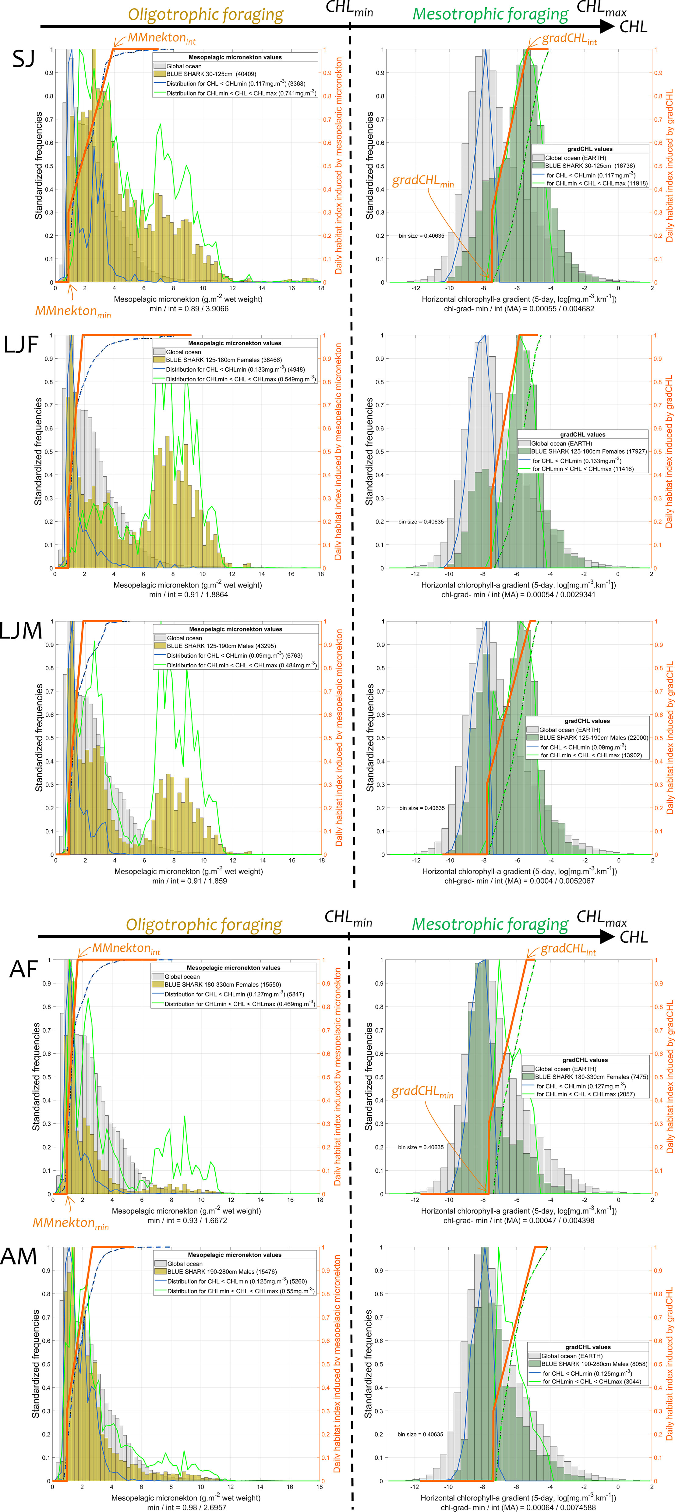
Figure 3 Frequency of blue shark presence in each foraging proxy (colored histograms, relative units) and identification of the respective daily linear function of foraging habitat (orange line segment). The distribution of mesopelagic micronekton (oligotrophic foraging, the colored histogram on left panels; MMnekton; g.m^-2 wet weight) and chlorophyll-a gradient (mesotrophic foraging, the colored histogram on the right panels; gradCHL; log-transformed, mg.m^-3.km^-1) at the location of blue shark presence data by size and sex classes (SJ, LJF, LJM, AF, and AM) are compared to the global ocean distribution (light grey histogram). The distribution of MMnekton and gradCHL at the location of blue shark presence and for CHL < CHL_min and CHL_min < CHL < CHL_max, respectively, are delineated by the blue and green lines. The maximum slope of the cumulative distribution of blue shark presence for each foraging proxy (blue and green dashed line for MMnekton and gradCHL, respectively) defines the slope of the daily habitat linear function (orange line; see also Table 1; also using MMnekton_min and gradCHL_min).

The Abiotic Niche

Using the abiotic variables to exclude unfavorable environments meant a large percentile range (0.3^th and 99.7^th percentile values, Table 2) for abiotic variables was required to encompass the extreme conditions of the Northwest Atlantic, which were under-sampled in our dataset and not sufficiently highlighted in the cluster analysis with two or three clusters only. The proximity of the cold Labrador Current to the warm Gulf Stream south of Nova Scotia (South-East Canada) during winter caused an extreme situation where the temperature of surface waters is colder (and fresher) than below the mixed layer. These SST levels are too cold for blue sharks (below about 11°C, Figure SM.16) yet are suitable at depth (T_mld+100above about 12°C). Because historic data (Campana et al., 2006) and some of our electronic tagging data demonstrate the substantial presence of blue sharks in winter in this area, we accounted for this peculiarity in the model by selecting the 0.3^th and 99.7^th percentile values of the global distribution by size and sex class for the range of SST and SSHa. This range was wide enough to suitably capture blue shark presence in that area (see regional validation in Figures SM.17-18). The parameterization of abiotic variables (Table 2) allows for tolerance of lower temperature levels, which was exhibited by the SJ and LJF classes (12.3°C and 11.6°C, respectively). Compared to the other classes, AM had the highest threshold to minimum temperature (14.8°C), indicating the lowest tolerance to cold temperatures. The maximum temperature tolerance is less variable among classes than the minimum, although adults display slightly higher levels than the other classes (c.f. 28.9-29.3°C with 28.3-28.6°C, Table 2). Similar to temperature, the preferred SSHa ranges of SJ and LJF classes are lower than the LJM and adult classes, indicating preferential use of highly productive and temperate areas than less productive and tropical areas. This can be seen by the differences in their frequency of presence in mesotrophic and oligotrophic environments (Figure 3). An unexpected pattern indicated by the environmental-presence data relationship was the apparent avoidance of large juveniles and adult females in an intermediate range of SST (Figure 4). Our results highlight that the presence of large females is three to four-fold lower than large males in the range of 21.7-24°C and 22.1-23.4°C for LJF and AF, respectively (5% presence for LJF compared to 17% for LJM, and 4% presence for AF compared to 13% for AM). These intermediate ranges of SST for LJF and AF were used to set the daily habitat to 0 (Table 2). To highlight the impact of this apparent avoidance by large females, we show the 21.7°C and 24°C isotherms on the mean seasonal habitat map for large males (next section).

TABLE 2

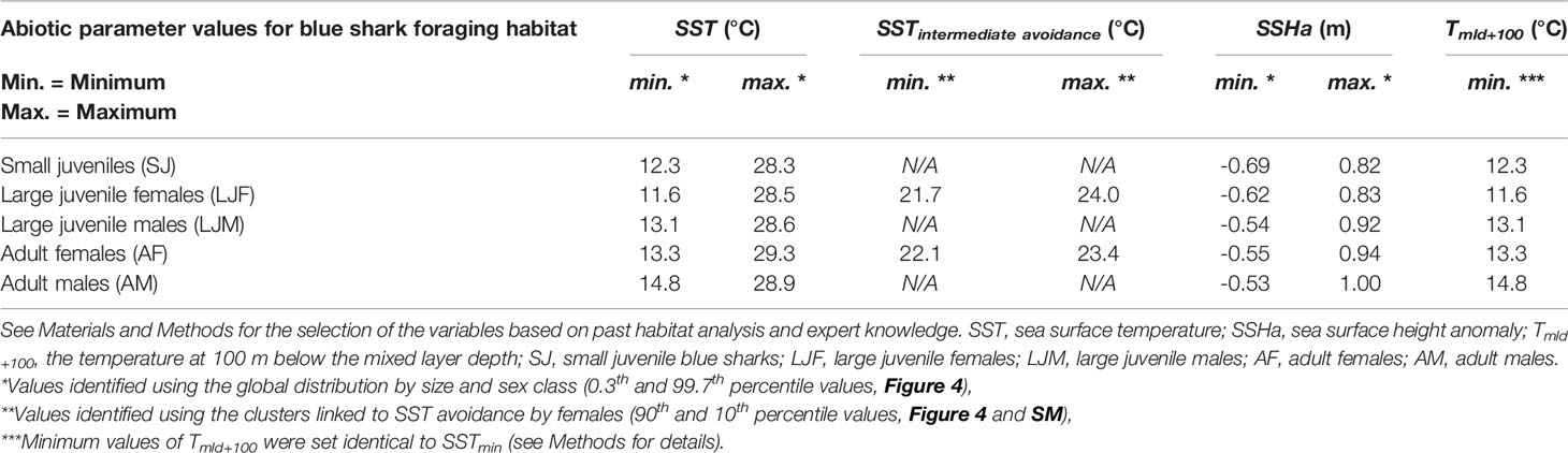
Table 2 Calibration parameters for the abiotic variables of the blue shark foraging habitat model.

FIGURE 4

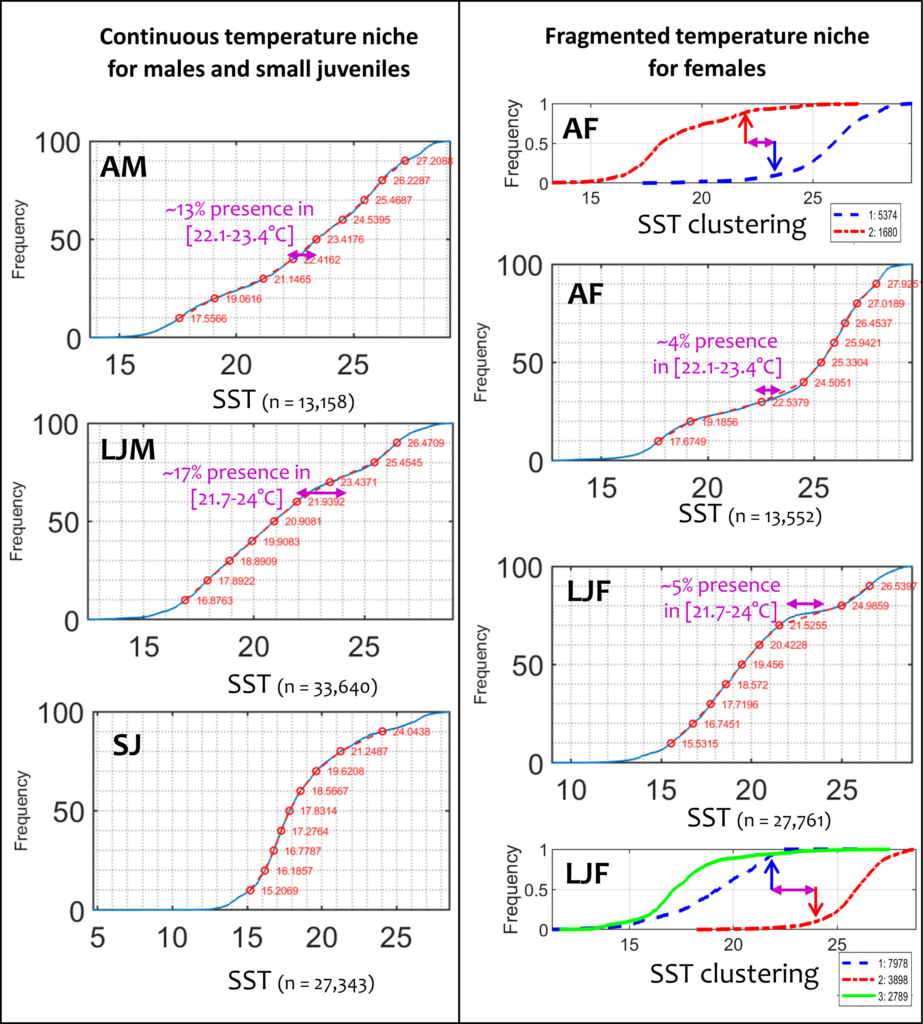
Figure 4 Global distribution of sea surface temperature (SST) by size and sex class of blue shark. A continuous SST niche for males and small juveniles (left panels) and a fragmented SST niche for large juvenile and adult females (right panels) is evident, with three to four-fold lower presence of females than males in the SST range of 21.7-24°C and 22.1-23.4°C, respectively.

Mean Seasonal Foraging Habitat by Sex and Size Class

We used the favorable foraging conditions of blue sharks for each class as defined by the model calibration to extrapolate daily global blue shark habitat. The mean seasonal foraging habitat by size and sex class for the period 2003-2018 was computed using monthly mean levels (Figures 5–9, see also Figure SM.6 for data integration and the seven habitat animations with the overlay of electronic tagging and observer data as separate SM). The frequency of suitable habitat occurrence (%) differed primarily among seasons and the five blue shark classes. We plotted the chlorophyll-a isocontour of CHL_min on each map to distinguish the distribution of foraging habitat arising from the mesopelagic micronekton (oligotrophic) and productivity front (mesotrophic) proxies (CHL < CHL_min and CHL_min < CHL < CHL_max, respectively). Oligotrophic environments tend to contain higher levels of suitable foraging habitat as compared to mesotrophic areas. This notably reflects the more stable estimated levels of mesopelagic micronekton compared to the scattered frequency of productivity fronts occurring in mesotrophic areas. Favorable conditions for oligotrophic foraging occur for all classes in the central part of the large subtropical gyres, although not in the most oligotrophic areas (see, e.g., the habitat differences between the subtropical northeast and poorer southeast Pacific, Figures 5-9). Instead, mesotrophic foraging mostly arises in temperate and equatorial latitudes, both of which display a seasonal contraction during the cold months alternately in both hemispheres, resulting in a latitudinal oscillation between the seasons in the equatorial area.

FIGURE 5

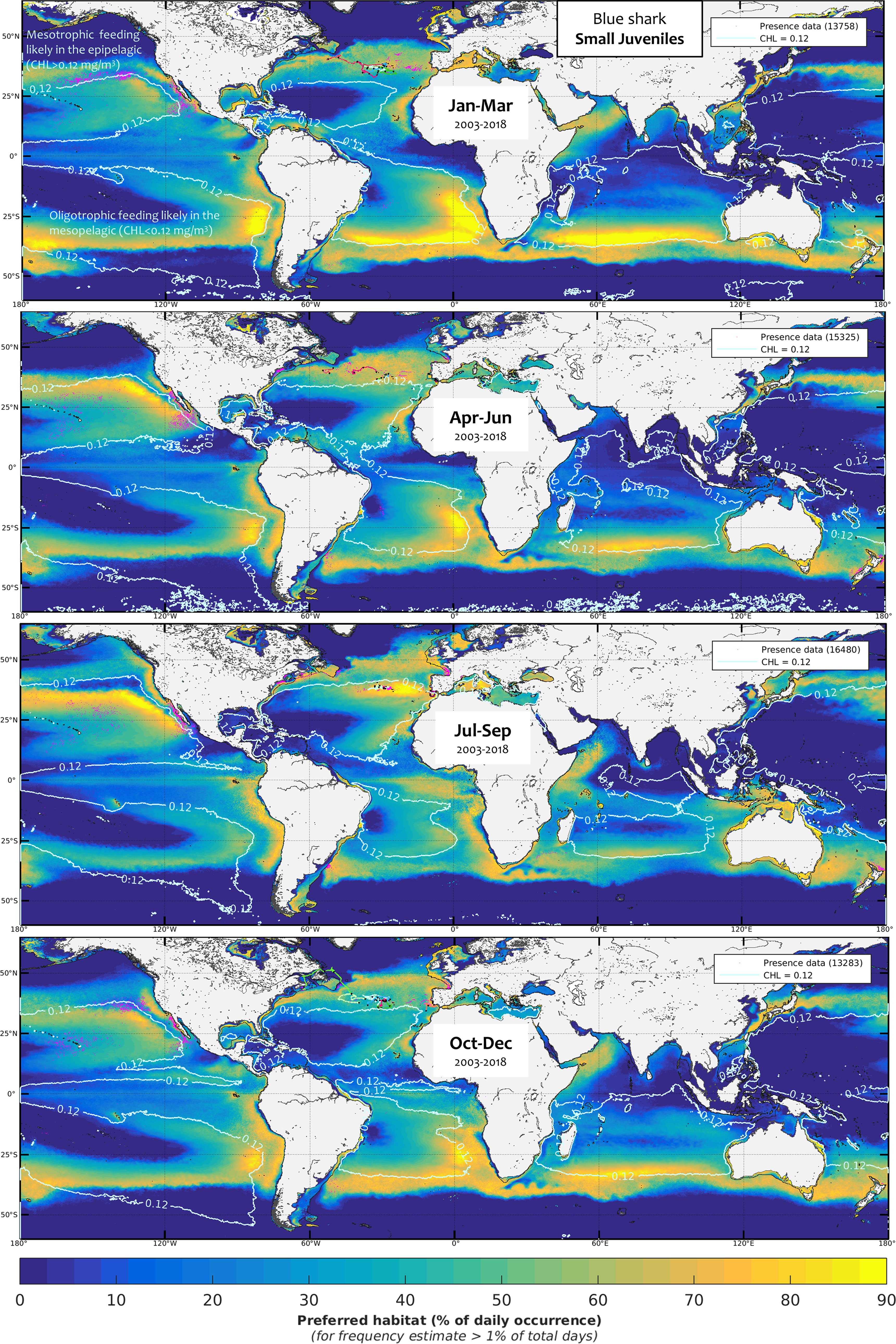
Figure 5 Mean seasonal distribution of blue shark foraging habitat for the small juveniles (SJ, 2003-2018, in frequency of suitable habitat occurrence, %). The chlorophyll-a isocontour of 0.12 mg.m^-3 (CHL_min) separates the mean area of oligotrophic foraging (below this value using mesopelagic micronekton as foraging proxy) and mesotrophic foraging (above this value using productivity fronts). Presence data (calibration and validation) are represented as pink dots for observer data and colored line transects for electronic tagging data (start and end of months are shown by a black star).

FIGURE 6

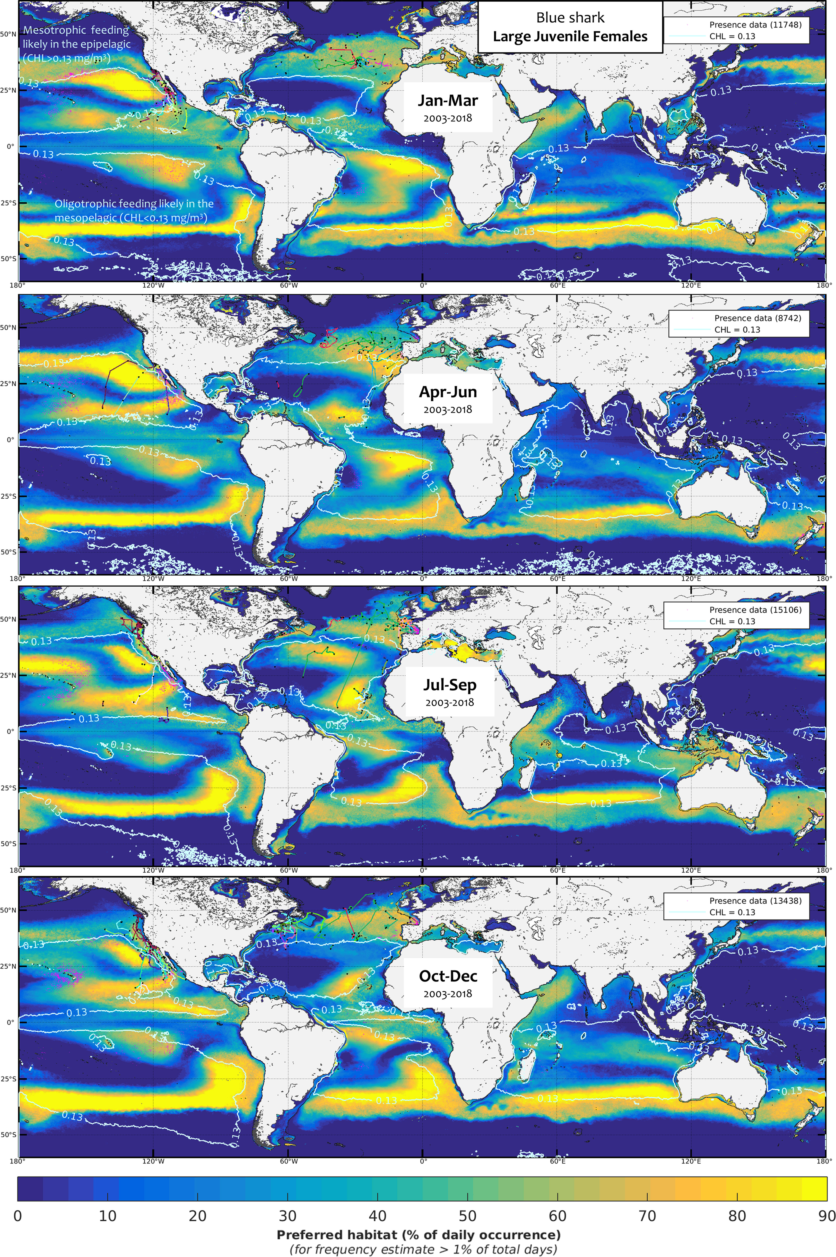
Figure 6 Mean seasonal distribution of blue shark foraging habitat for the large juvenile females (LJF, 2003-2018, in frequency of suitable habitat occurrence, %). The chlorophyll-a isocontour of 0.13 mg.m^-3 (CHL_min) separates the mean area of oligotrophic foraging (below this value using mesopelagic micronekton as foraging proxy) and mesotrophic foraging (above this value using productivity fronts). Presence data (calibration and validation) are represented as pink dots for observer data and colored line transects for electronic tagging data (start and end of months are shown by a black star).

FIGURE 7

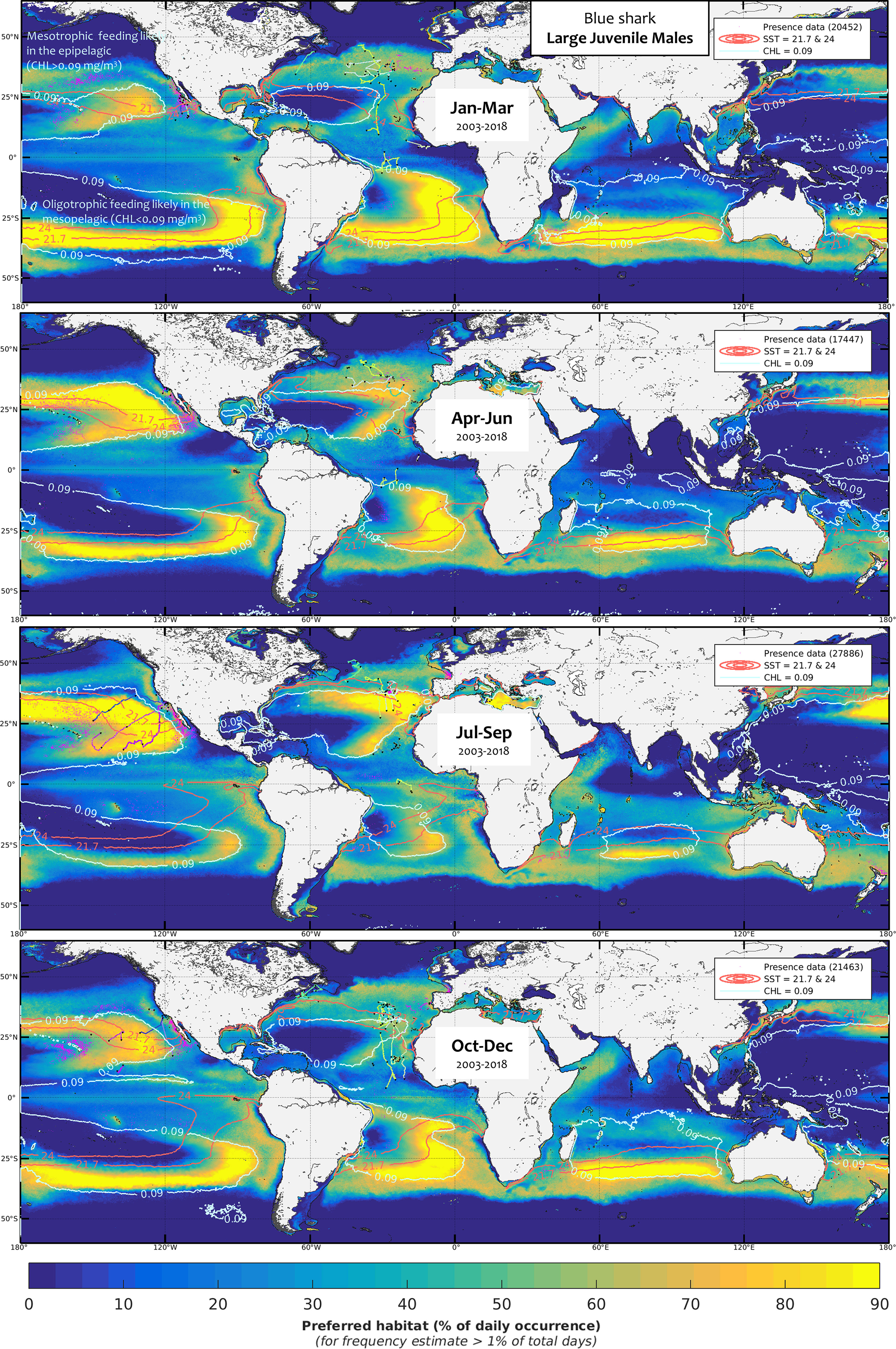
Figure 7 Mean seasonal distribution of blue shark foraging habitat for the large juvenile males (LJM, 2003-2018, in frequency of suitable habitat occurrence, %). The chlorophyll-a isocontour of 0.09 mg.m^-3 (CHL_min) separates the mean area of oligotrophic foraging (below this value using mesopelagic micronekton as foraging proxy) and mesotrophic foraging (above this value using productivity fronts). Presence data (calibration and validation) are represented as pink dots for observer data and colored line transects for electronic tagging data (start and end of months are shown by a black star). The SST isocontours of LJF avoidance (21.7°C and 24°C), slightly larger than for AF, allow evaluating the potential lack of habitat overlap with LJM.

FIGURE 8

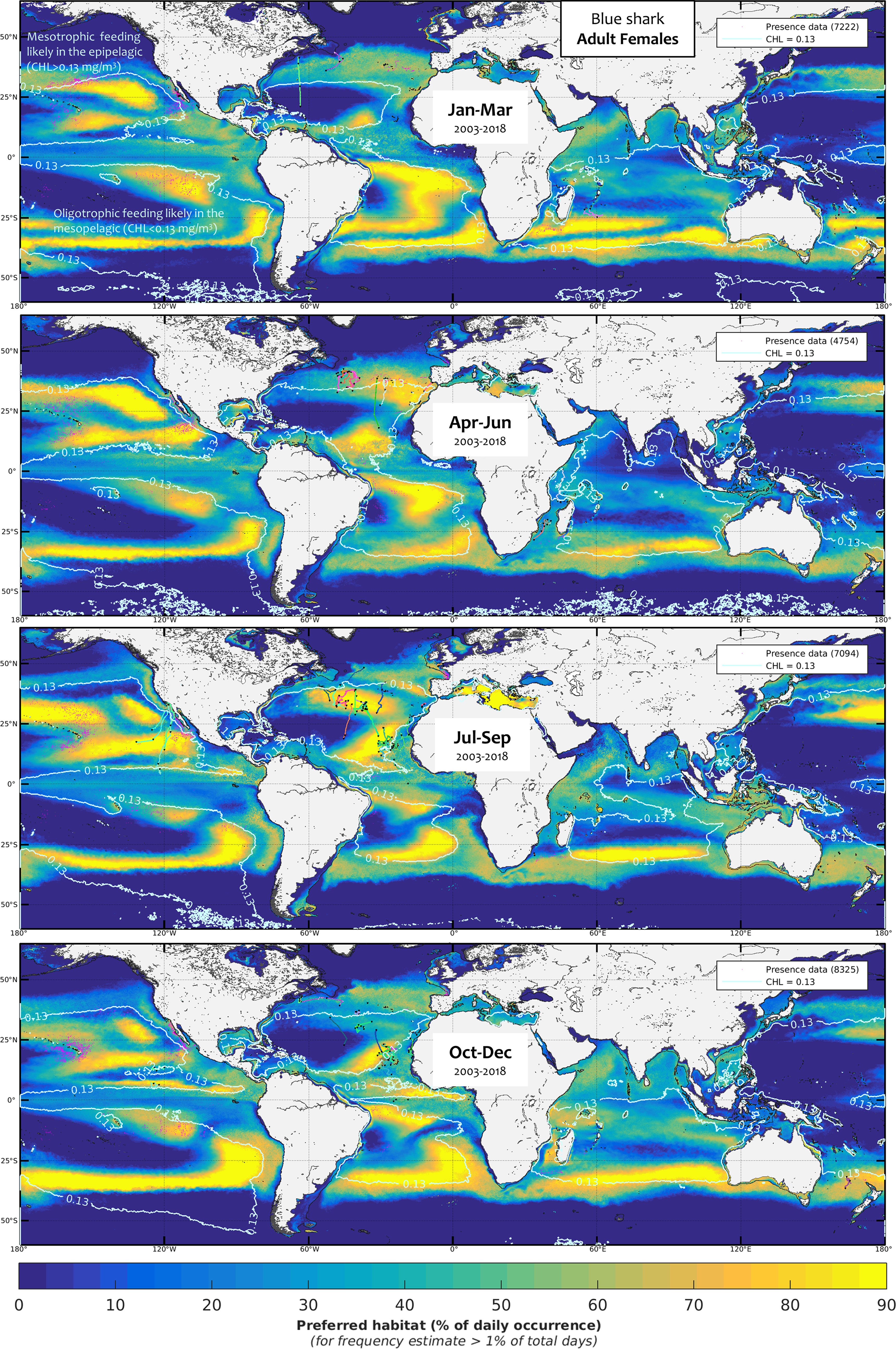
Figure 8 Mean seasonal distribution of blue shark foraging habitat for the adult females (AF, 2003-2018, in frequency of suitable habitat occurrence, %). The chlorophyll-a isocontour of 0.13 mg.m^-3 (CHL_min) separates the mean area of oligotrophic foraging (below this value using mesopelagic micronekton as foraging proxy) and mesotrophic foraging (above this value using productivity fronts). Presence data (calibration and validation) are represented as pink dots for observer data and colored line transects for electronic tagging data (start and end of months are shown by a black star).

FIGURE 9

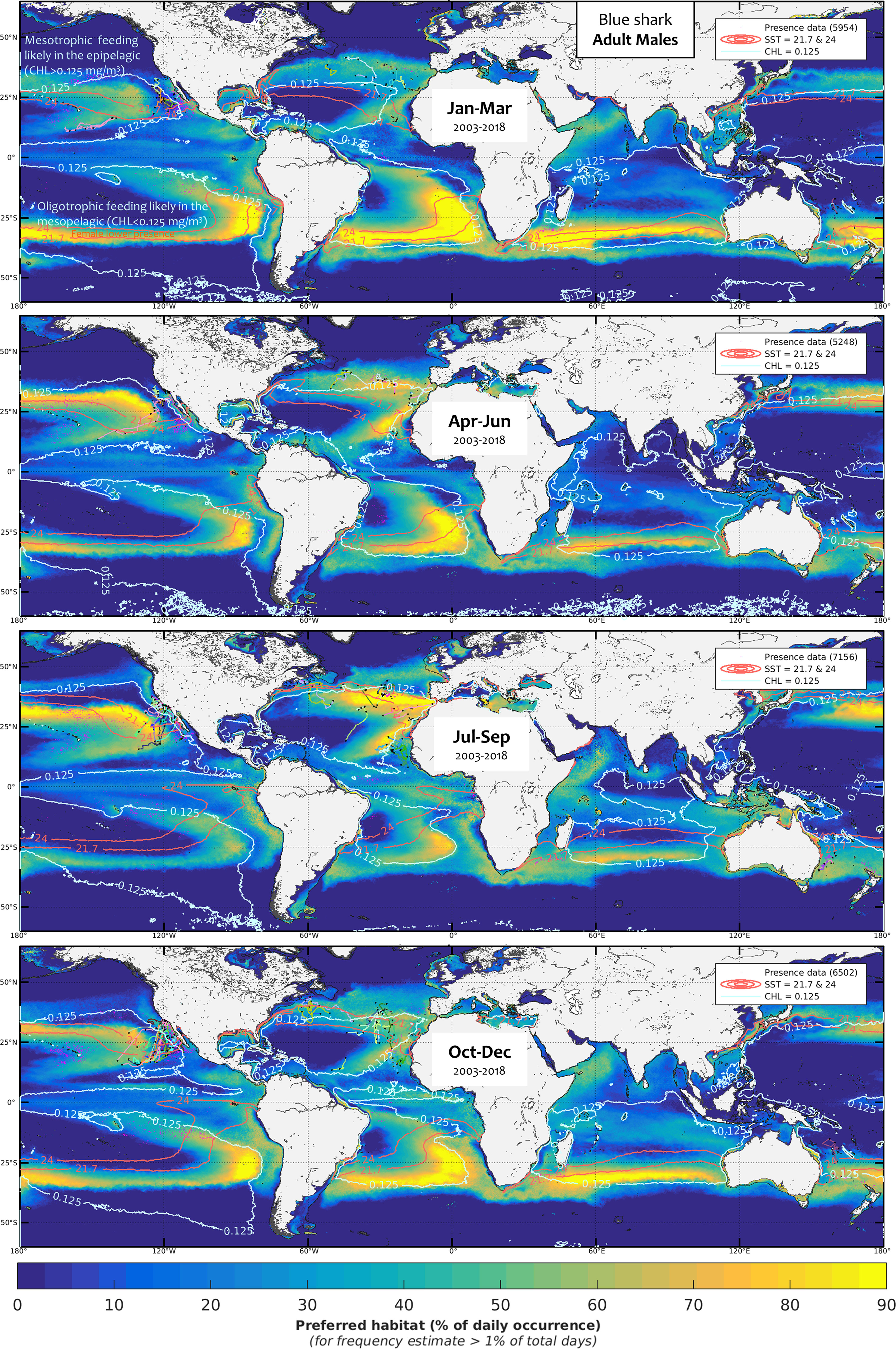
Figure 9 Mean seasonal distribution of blue shark foraging habitat for the adult males (AM, 2003-2018, in frequency of suitable habitat occurrence, %). The chlorophyll-a isocontour of 0.125 mg.m^-3 (CHL_min) separates the mean area of oligotrophic foraging (below this value using mesopelagic micronekton as foraging proxy) and mesotrophic foraging (above this value using productivity fronts). Presence data (calibration and validation) are represented as pink dots for observer data and colored line transects for electronic tagging data (start and end of months are shown by a black star). The SST isocontours of LJF avoidance (21.7°C and 24°C), slightly larger than for AF, allow evaluating the potential lack of habitat overlap with AM.

Although blue shark foraging habitat is generally widespread from about 50°S to 50°N, major unsuitable areas for foraging occur in the central part of the main tropical gyres, such as in the West and South-East Pacific or in the South-West of the North Atlantic Oceans, due to particularly low productivity and extremely high SSTs (Figures SM.13-15). In the Indian Ocean, SST is too high in the northern basin (see in Figure SM.14 the SST isocontour of 28.7°C enhancing the mean upper SST limitation between all classes, 28.7°C ±0.38) and productivity is too low in the latitudes from 15°S to 25°S (Figure SM.13). Given their more restricted temperature tolerances, a larger extent of the basin is unsuitable for males than for females, mostly due to higher SSTs than the tolerated levels (Figure SM.14). The SJ and AM classes show the most contrast in suitable environmental conditions and predicted foraging habitats, particularly in the northern hemisphere where seasonal variability is higher. For example, SJ has a higher latitudinal range in the North Pacific and Atlantic Oceans, yet a greater longitudinal range in the Mediterranean Sea since the western basin is further North. The other main difference between size and sex classes arises from the apparent avoidance of females in an intermediate range of SST levels. The SST avoidance isocontours of LJF shown on the mean seasonal maps of males (Figures 7, 9) highlight that habitat overlap between females and males is lacking mostly from January to June in the southern hemisphere, from April to December in the North Atlantic, and from July to March in the North Pacific. The overall observer and electronic tagging data generally agree well with the predicted lack of habitat overlap (see also Figures SM.22-24 comparing the males and females’ habitat with blue shark catches in (Coelho et al., 2018), except in specific areas and seasons (e.g., North-east Pacific in April-June, south-west Indian Ocean in October-December).

Global blue shark habitat declined during 2003-2018, as indicated by changes in the frequency of suitable habitat occurrence of about -0.13%.yr^-1, (Figure SM.26). Declines were unevenly distributed, with substantial negative trends (in excess of -1.5%.yr^-1 of favorable habitat occurrence) mostly in the northern and central Indian Ocean for the larger classes, and in the tropical northern Pacific Ocean. Habitat expansion into higher latitudes (above 30°) in both hemispheres was indicated by positive trends (in excess of -1.5%.yr^-1 in the North-west Atlantic, South Pacific and south Indian oceans). Overall, the higher losses of habitat over time for blue sharks appeared to occur in the equatorial and tropical Indian Ocean and in the tropical North Pacific, specifically for the juveniles. The major gains in habitat were observed in the Northwest Atlantic and the Mediterranean Sea for the larger size classes, and in the temperate South Pacific and Indian Oceans.

Distance of Presence Data to Closest Habitat and Seasonal Habitat Size

We used fairly strict minimum criteria for habitat coverage (see Materials and Methods and SM) to evaluate model performance from the independent validation data, representing 47% (125,825 observations) of the available information on blue shark presence (proportion by class ranges from 42 to 52%, Table SM.1). Globally, the validation data had a similar distribution as the calibration data, although with slightly higher representation in the North-East and South-East Pacific from additional longline observer data and in the North Atlantic from electronic tagging data. The model performance was estimated through i) the fraction of validation data within the highest quality habitat (where the minimum level for effective foraging was 30%, hereafter, core habitat), integrated over five days centered on the day of the observation, ii) the distance of 80% of the validation data to the closest core habitat boundary (how close to core habitat are most of the predator presence data) and iii) monthly changes in the relative surface of the core habitat to evaluate how discriminant the prediction is. The fraction of validation presence data within the core habitat reflects the potential for effective foraging, and was 74% for SJ (n = 25,563), 68% for LJM (n = 44,298), 58% for LJF (n = 26,366), 47% for AM (n = 14,004) and 61% for AF (n = 15,594). A predator searching for prey should remain in the vicinity of the core habitat, and the 80^th percentile of presence data to the closest core habitat boundary displayed the same ranking of performances by class: with 2 km for SJ, 3 km for LJM, 21 km for LJF, 29 km for AM and 10 km for AF (Figure 10).

FIGURE 10

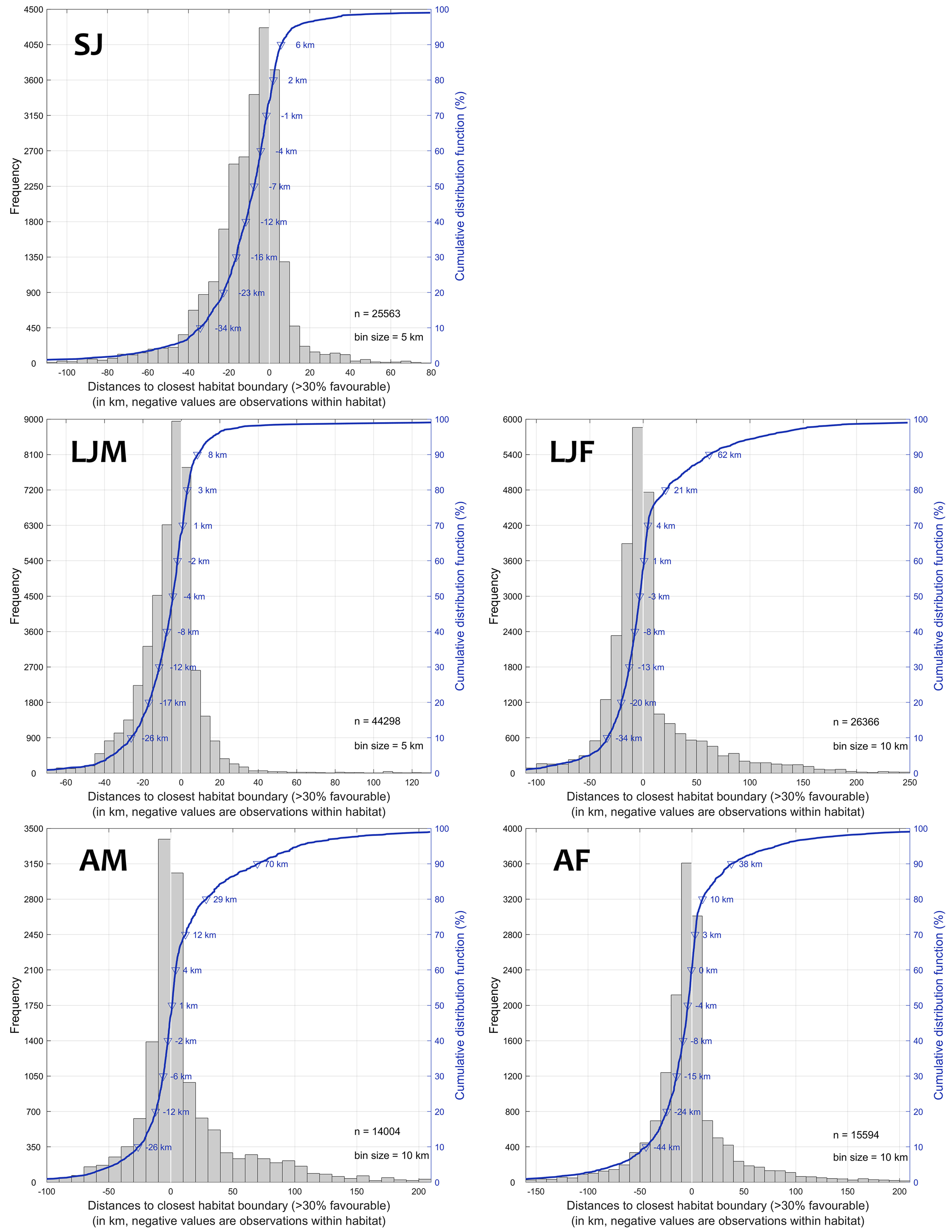
Figure 10 Model performance estimated in distances (km) of validation presence data to closest core habitat boundary (above 30% favorable) for each size and sex class (SJ, LJF, LJM, AF, and AM) and corresponding cumulative distribution showing distance values for each decile bin of presence data (negative are observations within favorable habitat). For the SJ class for instance, 74% of validation presence data were within the core habitat (above 30%) and the distance of the 80^th percentile of presence data to the closest core habitat boundary was 2 km (n = 25,563).

All classes present a large proportion of observations (86-99%) closer than 50 km, which matches the level of geolocation uncertainty of the presence data (Figure 10). This range is 79-97% between classes for observations closer than 25 km to the core habitat. Considering the large distribution of the species compared to the relatively low surface area of the predicted core habitat (about 18-22 ± 2% and 23-29 ± 2% in the north and south hemispheres, respectively, with larger and lower extents for SJ and AM, respectively, Figure SM.12), we conclude that the habitat model is fairly discriminant and accurately predicts habitat suitability among classes. Finally, we present in the SM as separate files seven regional habitat animations with the overlay of observer and electronic tagging data for a qualitative appreciation of the model results and a visualization of the seasonal movements of blue sharks by size and sex classes.

Discussion

Consistency of Model Results With Known Traits and Habitats

Quantitative validation associated with a relatively restricted surface area of the core habitat in the global ocean showed that the model can discriminate habitats by sex and size class for blue sharks. Furthermore, our results are consistent with previously published catch data in the contrasting SST conditions of the Northwest Atlantic (Figures SM.17-18, Campana et al., 2006) and in the central-eastern Atlantic, where a maximum of catch per unit of effort (CPUE, kg/set) corresponds to the spatial dominance of different habitat classes (Figures SM.19-20). At-sea observer data suggests large juvenile females predominate in relatively cold waters in the southeast Indian Ocean, which is consistent with our selected lower SST_min for this class than for males and adults (Figure SM.24). The model is qualitatively consistent with observations from other areas where little or no calibration data were used, especially in the Pacific Ocean. In the northwest Pacific, Nakano (1994) found a maximum CPUE of blue shark (in number for all classes) in the area 25-45°N, 140°E-160°W, with lower levels in the equatorial area (also in Strasburg, 1958). This pattern is well captured by the model (see interannual mean habitats in Figures SM.25). High CPUEs in number were observed to occur up to 55°N in the northeast Pacific in July (Nakano and Nagasawa, 1996), also in agreement with our results (Figures 5-9). Strasburg (1958) denoted a maximum CPUE of newborn blue sharks in the area 30-40°N in the Pacific in summer, which agrees with the highest habitat quality of the small juveniles for that season and represents the most persistent habitat in that region year-round (Figure 5). This observation of nurseries in the North Pacific is consistent with the presence of late-stage pregnant blue sharks in spring (30-40°N in the Northwest Pacific, Fujinami et al., 2021) and with the favorable habitat of adult females in the same season (Figure 8). In the Southwest Pacific, the mean prey biomass off eastern Australia is about nine-fold higher for blue sharks (n = 147, mean FL = 137 cm) south of 32°S compared to north (Young et al., 2010), which agrees well with our results for juveniles (Figures 5-7). In the tropical Southeast Pacific, our validation observer data matches well with the presence of large females (Figures 6, 8). Differences among sex and size classes are consistent with the observed size composition of blue shark catches in the Australasian region, with mostly juveniles south of 35°S and adults north of 35°S (West et al., 2004; Neubauer et al., 2021). The blue shark is the most landed shark species in the Peruvian shark fisheries, representing 42% of total landings (Gonzalez-Pestana et al., 2016), which indirectly corroborates our findings of suitable habitat for small juveniles and large females (Figure SM.25). In the Atlantic and Indian oceans, other catch data display consistent distributions with our results. Mostly adult blue sharks (195-320 cm total length) are caught by the artisanal driftnet fishery in the Guinea current (off Ivory Coast, Central-eastern Atlantic; (Konan et al., 2018), which correlates with the medium habitat quality of adults and the lack of favorable habitat of smaller specimens from our model (Figure SM.25). Notably, sex ratio and fork length distributions in the South Atlantic and the Indian Ocean lack female representation, which is consistent with the avoidance of intermediate SST by large females in the modeling (Figures SM.22-23). These intermediate SST levels also occur in the vicinity of the Azores (Figures 6, 8, and habitat animations in the SM), and large females are absent in catch data from July to November (Vandeperre et al., 2014b; Coelho et al., 2018).

The ecological benefit of sex segregation from females avoiding SST within their physiologically-tolerated range requires further investigation. It is possible that these environments correspond to suboptimal temperatures for pregnant blue sharks between the cooler parturition grounds and warmer subtropical waters, aiding fertilization and embryonic growth at the early development stage (Hazin et al., 1994; Fujinami et al., 2021). These intermediate SST levels likely correspond to poor nutritional conditions for pups compared to temperate waters (Nakano, 1994; Fujinami et al., 2021). These temperature levels may also correspond to the optimal temperature range for males’ gonad development and maturation (‘thermal-niche fecundity’, Wearmouth and Sims, 2008). Furthermore, large males are indiscriminate feeders (McCord and Campana, 2003), and could likely prey upon newly-born progeny if it would not be in the females’ evolutionary interest to stay away from males around the time of pupping. Finally, because of the aggressiveness of mating males and given the potential for injury (Sims, 2005), females may venture into these areas only when mating is strictly necessary. The twice-thicker skin of females (Pratt, 1979) could also result in higher tolerance to low temperatures (Vandeperre et al., 2014a), given that the LJF class had the lowest SST_min value (Table 2) compared to males. While temperature is fundamental to the habitat predictions, a direct comparison of minimum levels of averaged dive temperature (SST_min and T_mld+100) with absolute physiological thresholds in literature is difficult due to the high gradient of temperature experienced during the dives. Braun et al. (2019) reported a mean dive temperature of adult males in the relatively cold cyclonic eddies of about 15°C from tagging experiments in the Northwest Atlantic, which is consistent with our findings (14.8°C). Furthermore, blue sharks swiftly end their deep dives when muscle cools to 15°C, with a range of water temperature met during the dives spanning from 7 to 26°C (Carey et al., 1990). While finding the same minimum muscle temperature, Watanabe, Nakamura, and Chiang (Watanabe et al., 2021) concluded that the regular deep-diving behavior of this species can be parsimoniously explained by their motivation for maintaining body temperature within a narrow range while foraging in the stratified water columns. Overall, blue shark classes have variable tolerance to minimum temperature (LJF < SJ < [LJM, AF] < AM), which is valuable habitat information for identifying bycatch mitigation measures targeting the most vulnerable classes.

Approach Limitations

The accuracy of the blue shark niche and habitat prediction is limited by geolocation uncertainties of the observations, the intrinsic limitations of the environmental variables, and the necessary model simplification of a complex species ecology. The geolocation uncertainties of observer data and of the light/SST-derived electronic tagging, all may have influenced the precise identification of the ecological niche. Given the maximum length of longline sets (100km), it was not possible to determine a single location with a precision greater than 50 km. Similarly, the precision of light-based geolocation estimates in equatorial areas, in regions with low SST gradients, or during equinoxes in tropical areas can be low, even following estimation using Hidden Markov Models (Braun et al., 2015; Braun et al., 2018). We allowed for some positional inaccuracy by integrating each environmental variable within a 25 km radius (centered on the observations). Physiologically, blue sharks are likely able to explore such an area on a daily basis (Kai and Fujinami, 2020). Overall, both datasets (observer and electronic tagging) are complementary for describing the habitat niche since the fishery-dependent data are numerous and tends to be concentrated while the independent data are less frequent and more spread out. The optical remote sensing data from which CHL is derived is limited by cloud coverage, which frequently precludes data collection in relatively high latitudes (about 45-70°N) and in the equatorial belt. The effect of data gaps on habitat prediction was partially compensated for by using monthly habitat distributions to compute seasonal mean composites, therefore giving equal weight to each month. The other foraging proxy, the mesopelagic micronekton, has limitations inherent to the model used for its prediction. First, the parameters of the mesopelagic micronekton model were calibrated based on limited data, including observations derived from the literature (Lehodey et al., 2010), and trawling and acoustic survey data (GUID CMEMS, 2021). Although the optimization was successfully tested in this model, the biomass estimation from single-frequency acoustic data remains an issue for rigorous parameter estimation (Lehodey et al., 2015). Additionally, the empirical definition of the upper mesopelagic layer, which was based on the euphotic depth, needs to be further verified once complementary data become available.

Another limitation of the habitat model relates to the comparability of both foraging proxies. Large scale analysis of habitat quality is difficult because blue sharks modify their strategy over their lifespan, from more frequent foraging in relatively cold and mesotrophic waters (likely in the epipelagic layer) as a small juvenile, to less frequent and deeper foraging in relatively warm surface waters (likely in the mesopelagic layer) as an adult. Thus, habitat values do not represent absolute levels of foraging capacity in that they are not comparable in oligotrophic (micronekton, CHL < CHL_min) or mesotrophic conditions (CHL gradient, CHL_min < CHL < CHL_max). In other words, oligotrophic daily habitat values may reach the maximum value of 1 even if the foraging capacity is functionally much lower than in mesotrophic environments. Small juveniles and adults are both adapted to foraging in relatively productive/cold and poor/warm niches, respectively, to meet their energetic needs. This means that the habitat suitability represents both the foraging capacity within each proxy and the energetic needs of individuals. These characteristics of balanced energy intake and expenditure should be kept in mind when interpreting the habitat results. It should be further noted that the scaling of both foraging proxies was done independently from one another using the respective cumulative distribution functions of presence.

Finally, our decision to only use foraging proxies as attracting factors within the model means that biological processes such as reproduction are not explicitly accounted for. Because female parturition occurs in suitable environments for small juveniles (temperate waters, Nakano, 1994; Fujinami et al., 2021), we would expect a substantial overlap due to reproduction to be accounted for in our analyses. However, mating behavior may remain unaccounted for in the modeling if disconnected from foraging behavior. This might particularly be the case for AM for which the reproduction behavior may explain the lowest model performance among the five size and sex classes. Overall, the predicted habitat describes the suitable areas for foraging, and any organism allocates the energy obtained from it to the competing functions of growth, reproduction and longevity/survival (investment in maintenance, storage and repair, Litchman et al., 2013). These authors underline that organisms shall optimize their behavior and energy allocation pattern to maximize the fitness of the individual in a particular environment, which may apply to the blue shark foraging strategies in their lifespan from relatively cold and rich environments to warmer and poorer surface waters.

Perspectives for Research, Management, and Policy

There is an increasing need for appropriate management of blue shark stocks (e.g., in the Atlantic by ICCAT, European Union, 2020; European Union, 2021) due to greater fishing pressure in recent decades. While the species appears relatively resilient in some areas the catch of blue shark has dramatically declined in others. In the Atlantic, total catch has been relatively consistent over time (ICCAT, 2020) even though blue shark represents about 60% of the Spanish and Portuguese longline bycatch (Porsmoguer et al., 2015). Conversely, abundance in the Mediterranean Sea declined by 96.5% over 56 years (Ferretti et al., 2008). Furthermore, the level of uncertainty in the data inputs and structural model assumptions for blue shark stocks are often high enough to prevent reaching a consensus on specific management recommendations. Mitigation of shark bycatch mostly consists of measures related to fishing gears, specifying hook or lure or bait types, type of branch lines, and/or fishing depth (e.g., Sacchi, 2021) or prohibiting retention onboard, transhipment, landing or storing for certain sharks and fleets (e.g. IATTC Resolution C-19-05 for shark species). However, there is increasing interest from RFMOs to implement spatio-temporal management strategies (e.g., IOTC-2021-17^th Working Party on Ecosystems and Bycatch), especially under a dynamic management approach (e.g., Hazen et al., 2018; Lopez et al., 2019) that may highly reduce bycatch (Pons et al., 2022), which would require a good understanding of spatial population structure. Historically, the lack of long time-series of data specific to sex and size has limited the consideration of population structure (e.g. size and sex segregation) in stock assessment models (Mucientes et al., 2009). This means that any risk associated with differential fishing mortality rates on specific components of the stock cannot be accounted for. The data compiled for our study shows that morphological data are more readily available in recent years (53% of observations in our dataset, 2003-2018), which suggests that sex- and spatially-structured stock assessments could potentially be developed, elucidating the need for spatio-temporal measures to protect particularly vulnerable size and sex classes from fishing.

In general, blue sharks are relatively tolerant to the hardships of being hooked on a longline or entangled in a net for several hours but exhibit variable at-vessel mortality levels (3%, Kotas et al., 2000; 5%, Megalofonou et al., 2005; 4.9-31%, Hutchinson et al., 2021 and review herein) and higher post-release rates (15% with 95% CI, 8.5–25.1%, Musyl et al., 2011; 17% with 95% CI, 11-26%, Musyl and Gilman, 2019; 38%, Hutchinson et al., 2021) depending on the gear and regional practice. Coelho et al. (2012) also reported a relationship between mortality and size, with the smaller specimens having higher mortality rates than the larger sharks. Provided that best practices for handling and release are followed (Musyl and Gilman, 2019; Hutchinson et al., 2021), it is likely that releasing live blue sharks caught by longline fisheries is a complementary viable management tool to protect biomass in blue shark populations (as has been suggested in relation to the apparent recovery of the Southwest Pacific stock, Neubauer et al., 2021). It is likely mortality could be further reduced if spatio-temporal information on core habitats of the main life-history stages could be used to minimize catches of the most vulnerable classes. Vulnerability is likely greatest for small juveniles given their susceptibility to capture-induced mortality as well as adult females because they are pivotal to population productivity. As with any large elasmobranch, reproduction dynamics of blue shark are characterized by slow growth, late age of maturity and a relatively low reproductive rate (Myers and Worm, 2005). Spatio-temporal mitigation measures can also be related to depth. Depending on the specific longline fishery (e.g., the Canadian and Japanese longline fleets deploy gear within the top 15 m of the water column and at about 200 m, respectively), monthly mean habitat maps of the most vulnerable classes could highlight when the blue shark likely surface or exhibit mesopelagic foraging, using the CHL_min level as a boundary between both core habitats. Furthermore, it is noteworthy that young-of-the-year blue sharks spend most of their time at depths shallower than 40 m (Nosal et al., 2019) or that hooking lines in warm surface waters (e.g., > 28°C) may increase post-release mortality due to thermoregulation needs (Musyl and Gilman, 2018). Finally, temporal or spatial variation in stock structure, such as that provided by class-based habitat predictions, can improve specification of the selectivity pattern or growth models used in stock assessment, which can substantially reduce uncertainty in assessment results (Carvalho et al., 2015; Neubauer et al., 2021). There would also be the potential to use the extent and temporal trends of suitable habitats (Figures SM.25-26) to partially account for environmental variation affecting indices of abundance, to improve the standardization of catch per unit effort (Maunder et al., 2006). If strong inter-annual changes in habitats are detected, it would be meaningful to account for these habitat modifications in the stock projections used to determine catch advice, noting that substantial habitat trends (Figure SM.26) may serve as reasonable estimates for the near future. Our finding that suitable habitat extends poleward during the warm months and contracts during the cold months, as supported by satellite tracking, implies that blue shark populations may seasonally concentrate in the northern or southern basin ocean, alternately in both hemispheres, exhibiting higher vulnerability to fishing during periods when waters are the coldest (generally November-May and May-September in the north and south hemispheres, respectively, except the LJF class, see Figure SM.12). The decadal positive trend of habitat in high latitudes is likely due to the warming of surface waters, except for the negative trend in the subpolar North Atlantic where cooling was observed (Hu and Fedorov, 2020). A general poleward movement of the population and catches is likely to occur in the next decades. Future developments will focus on products for bycatch mitigation combining the core habitat of the classes to protect in priority (e.g. SJ and AF) with weights defined by management objectives. Such products, based on monthly habitat in the recent years, may serve as avoidance maps for fisheries, distinguishing with a color code the likely surface or deeper presence.

Understanding the ecological niche and core habitat of large pelagic species is key to promoting conservation and progressing in fishery management. We have shown how to incorporate environmental information available at suitable resolution together with detailed fisheries and fishery-independent data to meet this need at a global scale. Blue sharks, and other shark species even more vulnerable to fishing, should benefit from this approach, as it could be used to reduce uncertainty in stock assessment and inform different conservation and management options to ultimately promote long-term sustainability.

Data Availability Statement

The blue shark habitat data are available on the JRC Data Catalogue (https://data.jrc.ec.europa.eu/dataset?q=fish%20habitat) (or upon request) and habitat maps are available online (https://fishreg.jrc.ec.europa.eu/web/fish-habitat/habitatmapping). Chlorophyll-a data are available online (https://oceancolor.gsfc.nasa.gov/cgi/l3). The abiotic environmental and mesopelagic micronekton data are available online (https://marine.copernicus.eu/access-data).

Author Contributions

J-ND headed the collaboration and performed the computations. SC, FV, FH, HB, RC, NQ, FS, FA, DD, MM, JL, BB, PA, HD, PS, BF, AZ, PB, IS, FG, DS, JN, PC, AL, GD, MD, ER, and AJ analyzed the results, and wrote sections of the manuscript. SC, FV, FH, HB, RC, NQ, FS, FA, DD, MM, JL, BB, PA, HD, PS, BF, PB, IS, FG, DS, JN, PC, AL, GD, MZ, MD, ER, AJ, ML, MF, and PT provided data. All authors contributed to manuscript revision, read, and approved the submitted version.

Conflict of Interest

MM is employed by Pelagic Research Group LLC.

The remaining authors declare that the research was conducted in the absence of any commercial or financial relationships that could be construed as a potential conflict of interest.

Publisher’s Note

All claims expressed in this article are solely those of the authors and do not necessarily represent those of their affiliated organizations, or those of the publisher, the editors and the reviewers. Any product that may be evaluated in this article, or claim that may be made by its manufacturer, is not guaranteed or endorsed by the publisher.

Acknowledgments

The authors would like to particularly thank the following organizations and associated scientists for the data contributions on blue shark presence: Bedford Institute of Oceanography, Fisheries & Oceans Canada, Tagging of Pacific Pelagics - Packard and Moore Foundations (TOPP), National Oceanic and Atmospheric Administration (NOAA, Pacific Islands Regional Office, Honolulu, HI, and Southwest Fisheries Science Center, Monterey, CA), Inter-American Tropical Tuna Commission (IATTC), Instituto do Mar (IMAR), University of Azores, COSTA project (costaproject.org), Universidade Federal Rural de Pernambuco, Institut de Recherche pour le Développement (IRD), Pelagic Research Group Hawaii, Portuguese Institute for the Ocean and Atmosphere (IPMA), International Commission for the Conservation of Atlantic Tunas (ICCAT), AZTI, MEDLEM, Hellenic Centre for Marine Research (HCMR), MedBlueSGen project, CSIRO Marine and Atmospheric Research (Hobart), Ministry for Primary Industries – Fisheries New Zealand/National Institute of Water and Atmospheric Research (NIWA), Marine Biological Association of the UK, University of Southampton, CIBIO/In-BIO at the Universidade do Porto, Universidad Autónoma de Nuevo León/INAPESCA/PNAAPD/FIDEMAR, Indian Ocean Tuna Commission (IOTC), Spanish Institute of Oceanography (IEO), Organization of Associated Producers of Large Tuna Freezers (OPAGAC), University of Bari, Association Ailerons, Association des Requins et des Hommes. We also particularly thank the environmental data providers for the quality and availability of their ocean color products: NASA Ocean Biology (OB.DAAC), Greenbelt, MD, USA, and the EU-Copernicus Marine Environment Monitoring Service. The authors additionally thank Jose Blasco Munoz (EC-JRC) for the videos' editing. The authors are thankful to the reviewers for helping in editing the paper and providing valuable comments. This publication is dedicated to FH, he is and will be, missed for his extensive scientific knowledge, his contributions to improving shark management and conservation, and his exceptional human values and enthusiasm.

Supplementary Material

The Supplementary Material for this article can be found online at: https://www.frontiersin.org/articles/10.3389/fmars.2022.828412/full#supplementary-material

Supplementary Video 1 | LJF_NE_Pacific - Habitat animation with overlay of observations for large juvenile females of blue shark in the NE Pacific.

Supplementary Video 2 | LJM_N_Atlantic - Habitat animation with overlay of observations for large juvenile males of blue shark in the N Atlantic.

Supplementary Video 3 | AF_NE_Pacific - Habitat animation with overlay of observations for adult males of blue shark in the NE Pacific.

Supplementary Video 4 | AF_Indian_NW_Pacific - Habitat animation with overlay of observations for adult females of blue shark in the Indian and NW Pacific.

Supplementary Video 5 | AM_NE_Pacific - Habitat animation with overlay of observations for adult males of blue shark in the NE Pacific.

Supplementary Video 6 | SJ_N_Atlantic - Habitat animation with overlay of observations for small juveniles of blue shark in the N Atlantic.

Supplementary Video 7 | LJF_N_AtlanticHabitat animation with overlay of observations for large juvenile females of blue shark in the N Atlantic.

Supplementary Data Sheet 1 | Supplementary Information.

References

Adams G. D., Flores D., Galindo Flores O., Aarestrup K., Svendsen J. C. (2016). Spatial Ecology of Blue Shark and Shortfin Mako in Southern Peru: Local Abundance, Habitat Preferences and Implications for Conservation. Endanger. Species Res. 31, 19–32. doi: 10.3354/esr00744

CrossRef Full Text | Google Scholar

Aires-da-Silva A. M., Gallucci V. F. (2007). Demographic and Risk Analyses Applied to Management and Conservation of the Blue Shark (Prionace Glauca) in the North Atlantic Ocean. Marine Freshw. Res. 58 (6), 570–580. doi: 10.1071/MF06156

CrossRef Full Text | Google Scholar

Baudena A., Ser-Giacomi E., D’Onofrio D., Capet X., Cotté C., Cherel Y., et al. (2021). Fine-Scale Structures as Spots of Increased Fish Concentration in the Open Ocean. Sci. Rep. 11 (1), 1–13. doi: 10.1038/s41598-021-94368-1

PubMed Abstract | CrossRef Full Text | Google Scholar

Bigelow K. A., Boggs C. H., He X. I. (1999). Environmental Effects on Swordfish and Blue Shark Catch Rates in the US North Pacific Longline Fishery. Fish Oceanogr. 8 (3), 178–198. doi: 10.1046/j.1365-2419.1999.00105.x

CrossRef Full Text | Google Scholar

Braun C. D., Galuardi B., Thorrold S. R. (2018). HMMoce: An R Package for Improved Geolocation of Archival-Tagged Fishes Using a Hidden Markov Method. Methods Ecol. Evol. 9 (5), 1212–1220. doi: 10.1111/2041-210X.12959

CrossRef Full Text | Google Scholar

Braun C. D., Gaube P., Sinclair-Taylor T. H., Skomal G. B., Thorrold S. R. (2019). Mesoscale Eddies Release Pelagic Sharks From Thermal Constraints to Foraging in the Ocean Twilight Zone. Proc. Natl. Acad. Sci. 116 (35), 17187–17192. doi: 10.1073/pnas.1903067116

CrossRef Full Text | Google Scholar

Braun C. D., Kaplan M. B., Horodysky A. Z., Llopiz J. K. (2015). Satellite Telemetry Reveals Physical Processes Driving Billfish Behavior. Anim. Biotelem. 3 (1), 1–16. doi: 10.1186/s40317-014-0020-9

CrossRef Full Text | Google Scholar

Briscoe D. K., Hobday A. J., Carlisle A., Scales K., Paige Eveson J., Arrizabalaga H., et al. (2017). Ecological Bridges and Barriers in Pelagic Ecosystems. Deep Sea Res. Part II: Top Stud. Oceanogr. 140, 182–192. doi: 10.1016/j.dsr2.2016.11.004

CrossRef Full Text | Google Scholar

Calich H. J., Campana S. E. (2015). Mating Scars Reveal Mate Size in Immature Female Blue Shark Prionace Glauca. J. Fish Biol. 86 (6), 1845–1851. doi: 10.1111/jfb.12671

PubMed Abstract | CrossRef Full Text | Google Scholar

Campana S. E. (2016). Transboundary Movements, Unmonitored Fishing Mortality, and Ineffective International Fisheries Management Pose Risks for Pelagic Sharks in the Northwest Atlantic. Can. J. Fish Aquat. Sci. 73 (10), 1599–1607. doi: 10.1139/cjfas-2015-0502

CrossRef Full Text | Google Scholar

Campana S. E., Dorey A., Fowler M., Joyce W., Wang Z., Wright D., et al. (2011). Migration Pathways, Behavioural Thermoregulation and Overwintering Grounds of Blue Sharks in the Northwest Atlantic. PloS One 6 (2), e16854. doi: 10.1371/journal.pone.0016854

PubMed Abstract | CrossRef Full Text | Google Scholar

Campana S. E., Joyce W., Fowler M., Showell M. (2016). Discards, Hooking, and Post-Release Mortality of Porbeagle (Lamna Nasus), Shortfin Mako (Isurus Oxyrinchus), and Blue Shark (Prionace Glauca) in the Canadian Pelagic Longline Fishery. ICES J. Marine Sci. 73 (2), 520–528. doi: 10.1093/icesjms/fsv234

CrossRef Full Text | Google Scholar

Campana S. E., Marks L., Joyce W., Kohler N. E. (2006). Effects of Recreational and Commercial Fishing on Blue Sharks (Prionace Glauca) in Atlantic Canada, With Inferences on the North Atlantic Population. Can. J. Fish Aquat. Sci. 63 (3), 670–682. doi: 10.1139/f05-251

CrossRef Full Text | Google Scholar

Carey F. G., Scharold J. V., Kalmijn A. J. (1990). Movements of Blue Sharks (Prionace Glauca) in Depth and Course. Marine Biol. 106 (3), 329–342. doi: 10.1007/BF01344309

CrossRef Full Text | Google Scholar

Carpentieri P., Nastasi A., Sessa M., Srour eds A. (2021). Incidental Catch of Vulnerable Species in Mediterranean and Black Sea Fisheries – A Review. Gen. Fish Comm. Mediterr. Stud. Rev. 101, 320. doi: 10.4060/cb5405en

CrossRef Full Text | Google Scholar

Carvalho F., Ahrens R., Murie D., Bigelow K., Aires-Da-Silva A., Maunder M. N., et al. (2015). Using Pop-Up Satellite Archival Tags to Inform Selectivity in Fisheries Stock Assessment Models: A Case Study for the Blue Shark in the South Atlantic Ocean. ICES J. Marine Sci. 72 (6), 1715–1730. doi: 10.1093/icesjms/fsv026

CrossRef Full Text | Google Scholar

Carvalho F. C., Murie D. J., HV Hazin F., Hazin H. G., Leite-Mourato B., Burgess G. H. (2011). Spatial Predictions of Blue Shark (Prionace Glauca) Catch Rate and Catch Probability of Juveniles in the Southwest Atlantic. ICES J. Marine Sci. 68 (5), 890–900. doi: 10.1093/icesjms/fsr047

CrossRef Full Text | Google Scholar

Castro J. A., Mejuto J. (1995). Reproductive Parameters of Blue Shark, Prionace Glauca, and Other Sharks in the Gulf of Guinea. Marine Freshw. Res. 46 (6), 967–973. doi: 10.1071/MF9950967

CrossRef Full Text | Google Scholar

Castro J. I., Woodley C. M., Brudek R. L. (1999). “A Preliminary Evaluation of the Status of Shark Species,” in FAO Fisheries Techn. Pap, vol. 380. (Rome: FAO).

Google Scholar

Clarke S. C., McAllister M. K., Milner-Gulland E. J., Kirkwood G. P., Michielsens C. G. J., Agnew D. J., et al. (2006). Global Estimates of Shark Catches Using Trade Records From Commercial Markets. Ecol. Lett. 9 (10), 1115–1126. doi: 10.1111/j.1461-0248.2006.00968.x

PubMed Abstract | CrossRef Full Text | Google Scholar

Coelho R., Fernandez-Carvalho J., Lino P. G., Santos M. N. (2012). An Overview of the Hooking Mortality of Elasmobranchs Caught in a Swordfish Pelagic Longline Fishery in the Atlantic Ocean. Aquat. Living Resour. 25 (4), 311–319. doi: 10.1051/alr/2012030

CrossRef Full Text | Google Scholar

Coelho R., Mejuto J., Domingo A., Yokawa K., Liu K.-M., Cortés E., et al. (2018). Distribution Patterns and Population Structure of the Blue Shark (Prionace Glauca) in the Atlantic and Indian Oceans. Fish. Fish 19 (1), 90–106. doi: 10.1111/faf.12238

CrossRef Full Text | Google Scholar

Cordova-Zavaleta F., Mendo J., Briones-Hernandez S. A., Acuna-Perales N., Gonzalez-Pestana A., Alfaro-Shigueto J., et al. (2018). Food Habits of the Blue Shark, Prionace Glauca (Linnaeus 1758), in Waters Off Northern Peru. Fish. Bull. 116 (3–4), 310–324. doi: 10.7755/FB.116.3-4.9

CrossRef Full Text | Google Scholar

Cruz M. M., Elenara Szynwelski B., RO de Freitas T. (2021). Biodiversity on Sale: The Shark Meat Market Threatens Elasmobranchs in Brazil. Aquat. Conserv: Marine Freshw. Ecosyst., 1–14. doi: 10.1002/aqc.3710

CrossRef Full Text | Google Scholar

Desbiens A. A., Roff G., Robbins W. D., Taylor B. M., Castro-Sanguino C., Dempsey A., et al. (2021). Revisiting the Paradigm of Shark-Driven Trophic Cascades in Coral Reef Ecosystems. Ecology 102 (4), e03303. doi: 10.1002/ecy.3303

PubMed Abstract | CrossRef Full Text | Google Scholar

Dolgov A. V., Drevetnyak K. V., Gusev E. V. (2005). The Status of Skate Stocks in the Barents Sea. J. Northwest Atlantic Fishery Sci. 35, 249–260. doi: 10.2960/J.v35.m522

CrossRef Full Text | Google Scholar

Druon J.-N., Chassot E., Murua H., Lopez J. (2017). Skipjack Tuna Availability for Purse Seine Fisheries Is Driven by Suitable Feeding Habitat Dynamics in the Atlantic and Indian Oceans. Front. Marine Sci. 4. doi: 10.3389/fmars.2017.00315

CrossRef Full Text | Google Scholar

Druon J.-N., Fromentin J.-M., Hanke A. R., Arrizabalaga H., Damalas D., Tičina V., et al. (2016). Habitat Suitability of the Atlantic Bluefin Tuna by Size Class: An Ecological Niche Approach. Prog. Oceanogr. 142, 30–46. doi: 10.1016/j.pocean.2016.01.002

CrossRef Full Text | Google Scholar

Druon J.-N., Gascuel D., Gibin M., Zanzi A., Fromentin J.-M., Colloca F., et al. (2021). Mesoscale Productivity Fronts and Local Fishing Opportunities in the European Seas. Fish Fish 22, 1227–1247. doi: 10.1111/faf.12585

CrossRef Full Text | Google Scholar

Druon J.-N., Hélaouët P., Beaugrand G., Fromentin J.-M., Palialexis A., Hoepffner N. (2019). Satellite-Based Indicator of Zooplankton Distribution for Global Monitoring. Sci. Rep. 9 (1), 1–13. doi: 10.1038/s41598-019-41212-2

PubMed Abstract | CrossRef Full Text | Google Scholar

Dulvy N. K., Pacoureau N., Rigby C. L., Pollom R. A., Jabado R. W., Ebert D. A., et al. (2021). Overfishing Drives Over One-Third of All Sharks and Rays Toward a Global Extinction Crisis. Curr. Biol. 31 (21), 4773–4787. doi: 10.1016/j.cub.2021.08.062

PubMed Abstract | CrossRef Full Text | Google Scholar

Elliott R. (2020). “Spatio-Temporal Patterns in Movement, Behaviour and Habitat Use by a Pelagic Predator, the Blue Shark (Prionace Glauca), Assessed Using Satellite Tags.” University of Auckland, New Zealand: PhD Thesis, ResearchSpace@ Auckland.

Google Scholar

European Union (2020). “COUNCIL REGULATION (EU) 2020/123 of 27 January 2020 Fixing for 2020 the Fishing Opportunities for Certain Fish Stocks and Groups of Fish Stocks, Applicable in Union Waters and, for Union Fishing Vessels, in Certain Non-Union Waters”. Official Journal of the European Union.

Google Scholar

European Union (2021). “COUNCIL REGULATION (EU) 2021/92 of 28 January 2021 Fixing for 2021 the Fishing Opportunities for Certain Fish Stocks and Groups of Fish Stocks, Applicable in Union Waters and, for Union Fishing Vessels, in Certain Non-Union Waters.”

Google Scholar

Ferretti F., Myers R. A., Serena F., Lotze H. K. (2008). Loss of Large Predatory Sharks From the Mediterranean Sea. Conserv. Biol. 22 (4), 952–964. doi: 10.1111/j.1523-1739.2008.00938.x

PubMed Abstract | CrossRef Full Text | Google Scholar

Ferretti F., Worm B., Britten G. L., Heithaus M. R., Lotze H. K. (2010). Patterns and Ecosystem Consequences of Shark Declines in the Ocean. Ecol. Lett. 13 (8), 1055–1071. doi: 10.1111/j.1461-0248.2010.01489.x

PubMed Abstract | CrossRef Full Text | Google Scholar

Frid A., Baker G., Dill L. (2008). Do Shark Declines Create Fear-Released Systems? Oikos 117 (2), 191–201. doi: 10.1111/j.2007.0030-1299.16134.x

CrossRef Full Text | Google Scholar

Fujinami Y., Shiozaki K., Hiraoka Y., Semba Y., Ohshimo S., Kai M. (2021). Seasonal Migrations of Pregnant Blue Sharks Prionace Glauca in the Northwestern Pacific. Marine Ecol. Prog. Ser. 658, 163–179. doi: 10.3354/meps13557

CrossRef Full Text | Google Scholar

Godø O. R., Samuelsen A., Macaulay G. J., Patel R., Sætre Hjøllo S., Horne J., et al. (2012). Mesoscale Eddies Are Oases for Higher Trophic Marine Life. PloS One 7 (1), e30161. doi: 10.1371/journal.pone.0030161

PubMed Abstract | CrossRef Full Text | Google Scholar

Gonzalez-Pestana A., Kouri C., Velez-Zuazo X. (2016). Shark Fisheries in the Southeast Pacific: A 61-Year Analysis From Peru. F1000Research 3, 164. doi: 10.12688/f1000research.4412.2

CrossRef Full Text | Google Scholar

GUID CMEMS. (2021). “GLOBAL_MULTIYEAR_BGC_001_033, Quality Information Document.” Available at: https://catalogue.marine.copernicus.eu/documents/QUID/CMEMS-GLO-QUID-001-033.pdf.

Google Scholar

Hazen E. L., Scales K. L., Maxwell S. M., Briscoe D. K., Welch H., Bograd S. J., et al. (2018). A Dynamic Ocean Management Tool to Reduce Bycatch and Support Sustainable Fisheries. Sci. Adv. 4 (5), eaar3001. doi: 10.1126/sciadv.aar3001

PubMed Abstract | CrossRef Full Text | Google Scholar

Hazin F., Kihara K., Otsuka K., Boeckman C. E., Leal E. C. (1994). Reproduction of the Blue Shark Prionace Glauca in the South-Western Equatorial Atlantic Ocean. Fish Sci. 60 (5), 487–915. doi: 10.2331/fishsci.60.487

CrossRef Full Text | Google Scholar

Holden M. J. (1974). Problems in the Rational Exploitation of Elasmobranch Populations and Some Suggested Solutions. Sea Fish Res. 117–37.

Google Scholar

Hu S., Fedorov A. V. (2020). Indian Ocean Warming as a Driver of the North Atlantic Warming Hole. Nat. Commun. 11 (1), 1–11. doi: 10.1038/s41467-020-18522-5

PubMed Abstract | CrossRef Full Text | Google Scholar

Hu C., Lee Z., Franz B. (2012). Chlorophyll a Algorithms for Oligotrophic Oceans: A Novel Approach Based on Three-Band Reflectance Difference. J. Geophys. Res.: Oceans 117 (C1), 1–25. doi: 10.1029/2011JC007395

CrossRef Full Text | Google Scholar

Hutchinson M., Siders Z., Stahl J., Bigelow K. (2021). Quantitative Estimates of Post-Release Survival Rates of Sharks Captured in Pacific Tuna Longline Fisheries Reveal Handling and Discard Practices That Improve Survivorship. PIFSC Data Rep., DR-21-001. doi: 10.25923/0m3c-2577

CrossRef Full Text | Google Scholar

ICCAT (2015) “Report of the 2015 ICCAT Blue Shark Stock Assessment Session.” ICCAT Madrid. Available at: https://www.iccat.int/Documents/SCRS/DetRep/BSH_SA_ENG.PDF.

Google Scholar

ICCAT (2020) “Report for Biennial Period 2018-19 PART II, Madrid, Spain.” Collective Volume of Scientific Papers ICCAT 2 (SCRS). Available at: https://www.iccat.int/Documents/BienRep/REP_EN_18-19_II-2.pdf.

Google Scholar

Kai M., Fujinami Y. (2020). Estimation of Mean Movement Rates for Blue Sharks in the Northwestern Pacific Ocean. Anim. Biotelem. 8 (1), 1–8. doi: 10.1186/s40317-020-00223-x

CrossRef Full Text | Google Scholar

Konan K. J., Yves-Narcisse Kouamé K., Issa Ouattara N., Koné T. (2018). Feeding Habits of the Blue Shark Prionace Glauca (Linnaeu) Off the Coastal Waters of Ivory Coast (West Africa). J. Biodivers. Environ. Sci. (JBES) 12 (3), 192–200.

Google Scholar

Kotas J. E., dos Santos S., Guedes de Azevedo V., Meneses de Lima J. H., Dias Neto J., Fernández Lin C. (2000). Observations on Shark By-Catch in the Monofilament Longline Fishery Off Southern Brazil and the National Ban on Finning. IBAMA–REVIZEE Res. 8.

Google Scholar

Lehodey P., Conchon A., Senina I., Domokos R., Calmettes B., Jouanno J., et al. (2015). Optimization of a Micronekton Model With Acoustic Data. ICES J. Marine Sci. 72 (5), 1399–1412. doi: 10.1093/icesjms/fsu233

CrossRef Full Text | Google Scholar

Lehodey P., Murtugudde R., Senina I. (2010). Bridging the Gap From Ocean Models to Population Dynamics of Large Marine Predators: A Model of Mid-Trophic Functional Groups. Prog. Oceanogr. 84 (1), 69–84. doi: 10.1016/j.pocean.2009.09.008

CrossRef Full Text | Google Scholar

Litchman E., Ohman M. D., Kiørboe T. (2013). Trait-Based Approaches to Zooplankton Communities. J. Plankton Res. 35 (3), 473–484. doi: 10.1093/plankt/fbt019

CrossRef Full Text | Google Scholar

Lopez J., Lennert-Cody C., Maunder M., Xu H., Brodie S., Jacox M., et al. (2019). “Developing Alternative Conservation Measures for Bigeye Tuna in the Eastern Pacific Ocean: A Dynamic Ocean Management Approach,” in American Fisheries Society & The Wildlife Society 2019 Joint Annual Conference. AFS. Available at: https://www.iattc.org/Meetings/Meetings2019/SAC-10/INF/_English/SAC-10-INF-D_Bigeye%20tuna%20Dynamic%20Ocean%20Management.pdf.

Google Scholar

Mancusi C., Baino R., Fortuna C., Gil De Sola L., Morey G., Nejmeddine Bradai M., et al. (2020) “MEDLEM Database, a Data Collection on Large Elasmobranchs in the Mediterranean and Black Seas.” Available at: 10.12681/mms.21148.

CrossRef Full Text | Google Scholar

Maunder M. N., Sibert J. R., Fonteneau A., Hampton J., Kleiber P., Harley S. J. (2006). Interpreting Catch Per Unit Effort Data to Assess the Status of Individual Stocks and Communities. ICES J. Marine Sci. 63 (8), 1373–1385. doi: 10.1016/j.icesjms.2006.05.008

CrossRef Full Text | Google Scholar

Maxwell S. M., Scales K. L., Bograd S. J., Briscoe D. K., Dewar H., Hazen E. L., et al. (2019). Seasonal Spatial Segregation in Blue Sharks (Prionace Glauca) by Sex and Size Class in the Northeast Pacific Ocean. Divers. Distrib. 25 (8), 1304–1317. doi: 10.1111/ddi.12941

CrossRef Full Text | Google Scholar

McCord M. E., Campana S. E. (2003). A Quantitative Assessment of the Diet of the Blue Shark (Prionace Glauca) Off Nova Scotia, Canada. J. Northwest Atlantic Fishery Sci. 32, 57–63. doi: 10.2960/J.v32.a4

CrossRef Full Text | Google Scholar

Megalofonou P., Damalas D., De Metrio G. (2009). Biological Characteristics of Blue Shark, Prionace Glauca, in the Mediterranean Sea. J. Marine Biol. Assoc. United Kingdom 89 (6), 1233–1242. doi: 10.1017/S0025315409000216

CrossRef Full Text | Google Scholar

Megalofonou P., Damalas D., Yannopoulos C., De Metrio G., Deflorio M., de la Serna J. M., et al. (2000). By Catches and Discards of Sharks in the Large Pelagic Fisheries in the Mediterranean Sea. Final Rep. Project 97/50.

Google Scholar

Megalofonou P., Yannopoulos C., Damalas D., De Metrio G., de la Serna J. M., Macias D. (2005). Incidental Catch and Estimated Discards of Pelagic Sharks From the Swordfish and Tuna Fisheries in the Mediterranean Sea. Fish. Bull. 103 (4), 620–634.

Google Scholar

Miller P. I., Scales K. L., Ingram S. N., Southall E. J., Sims D. W. (2015). Basking Sharks and Oceanographic Fronts: Quantifying Associations in the North-East Atlantic. Funct. Ecol. 29 (8), 1099–1109. doi: 10.1111/1365-2435.12423

CrossRef Full Text | Google Scholar

Mucientes G. R., Queiroz N., Sousa L. L., Tarroso P., Sims D. W. (2009). Sexual Segregation of Pelagic Sharks and the Potential Threat From Fisheries. Biol. Lett. 5 (2), 156–159. doi: 10.1098/rsbl.2008.0761

PubMed Abstract | CrossRef Full Text | Google Scholar

Musick J. A., Burgess G., Cailliet G., Camhi M., Fordham S. (2000). Management of Sharks and Their Relatives (Elasmobranchii). Fisheries 25 (3), 9–13. doi: 10.1577/1548-8446(2000)025<0009:MOSATR>2.0.CO;2

CrossRef Full Text | Google Scholar

Musyl M. K., Brill R. W., Curran D. S., Fragoso N. M., McNaughton L. M., Nielsen A., et al. (2011). Postrelease Survival, Vertical and Horizontal Movements, and Thermal Habitats of Five Species of Pelagic Sharks in the Central Pacific Ocean. Fish. Bull. 109 (4), 341–368.

Google Scholar

Musyl M. K., Gilman E. L. (2018). Post-Release Fishing Mortality of Blue (Prionace Glauca) and Silky Shark (Carcharhinus Falciformes) From a Palauan-Based Commercial Longline Fishery. Rev. Fish Biol. Fish 28 (3), 567–586. doi: 10.1007/s11160-018-9517-2

CrossRef Full Text | Google Scholar

Musyl M. K., Gilman E. L. (2019). Meta-Analysis of Post-Release Fishing Mortality in Apex Predatory Pelagic Sharks and White Marlin. Fish Fish 20 (3), 466–500. doi: 10.1111/faf.12358

CrossRef Full Text | Google Scholar

Myers R. A., Worm B. (2005). Extinction, Survival or Recovery of Large Predatory Fishes. Philos. Trans. R. Soc. B: Biol. Sci. 360 (1453), 13–20. doi: 10.1098/rstb.2004.1573

CrossRef Full Text | Google Scholar

Nakano H. (1994). Age, Reproduction and Migration of Blue Shark [Prionace] in the North Pacific Ocean. Bulletin-National Res. Institute Far Seas Fish (Japan) 31, 141–256.

Google Scholar

Nakano H., Nagasawa K. (1996). Distribution of Pelagic Elasmobranchs Caught by Salmon Research Gillnets in the North Pacific. Fish Sci. 62 (6), 860–865. doi: 10.2331/fishsci.62.860

CrossRef Full Text | Google Scholar

Neubauer P., Large K., Brouwer S. (2021). Stock Assessment of Southwest Pacific Blue Shark,” WCPFC-SC17-2021/SA-WP-03. Report to the WCPFC Scientific Committee. Seventeenth Regular Session, 66.

Google Scholar

Nosal A. P., Cartamil D. P., Wegner N. C., Lam C. H., Hastings P. A. (2019). Movement Ecology of Young-Of-the-Year Blue Sharks Prionace Glauca and Shortfin Makos Isurus Oxyrinchus Within a Putative Binational Nursery Area. Marine Ecol. Prog. Ser. 623, 99–115. doi: 10.3354/meps13021

CrossRef Full Text | Google Scholar

Okes N., Sant G. (2019). An Overview of Major Shark Traders, Catchers and Species. TRAFFIC Cambridge UK.

Google Scholar

Olson D. B., Hitchcock G. L., Mariano A. J., Ashjian C. J., Peng G., Nero R. W., et al. (1994). Life on the Edge: Marine Life and Fronts. Oceanography 7 (2), 52–60. doi: 10.5670/oceanog.1994.03

CrossRef Full Text | Google Scholar

Pacoureau N., Rigby C. L., Kyne P. M., Sherley R. B., Winker H., Carlson J. K., et al. (2021). Half a Century of Global Decline in Oceanic Sharks and Rays. Nature 589 (7843), 567–571. doi: 10.1038/s41586-020-03173-9

PubMed Abstract | CrossRef Full Text | Google Scholar

Panigada S., Donovan G. P., Druon J.-N., Lauriano G., Pierantonio N., Pirotta E., et al. (2017). Satellite Tagging of Mediterranean Fin Whales: Working Towards the Identification of Critical Habitats and the Focussing of Mitigation Measures. Sci. Rep. 7 (1), 1–12. doi: 10.1038/s41598-017-03560-9

PubMed Abstract | CrossRef Full Text | Google Scholar

Polovina J. J., Howell E., Kobayashi D. R., Seki M. P. (2001). The Transition Zone Chlorophyll Front, a Dynamic Global Feature Defining Migration and Forage Habitat for Marine Resources. Prog. Oceanogr. 49 (1–4), 469–483. doi: 10.1016/S0079-6611(01)00036-2

CrossRef Full Text | Google Scholar

Pons M., Watson J. T., Ovando D., Andraka S., Brodie S., Domingo A., et al. (2022). Trade-Offs Between Bycatch and Target Catches in Static Versus Dynamic Fishery Closures. Proc. Natl. Acad. Sci. 119, (4). doi: 10.1073/pnas.2114508119

CrossRef Full Text | Google Scholar

Porcher I. F., Darvell B. W., Ziegler I. (2021). Shark Conservation–Analysis and Synthesis. Preprints doi: 10.20944/preprints202102.0145.v4

CrossRef Full Text | Google Scholar

Porsmoguer S. B., Bănaru D., Boudouresque C. F., Dekeyser I., Almarcha C. (2015). Hooks Equipped With Magnets Can Increase Catches of Blue Shark (Prionace Glauca) by Longline Fishery. Fish Res. 172, 345–351. doi: 10.1016/j.fishres.2015.07.016

CrossRef Full Text | Google Scholar

Pratt HAROLD L. (1979). Reproduction in the Blue Shark, Prionace Glauca. Fishery Bull. 77 (2), 445–470.

Google Scholar

Queiroz N., Humphries N. E., Couto A., Vedor M., Da Costa I., MM Sequeira A., et al. (2019). Global Spatial Risk Assessment of Sharks Under the Footprint of Fisheries. Nature 572 (7770), 461–466. doi: 10.1038/s41586-019-1444-4

PubMed Abstract | CrossRef Full Text | Google Scholar

Queiroz N., Humphries N. E., Noble L. R., Santos A. M., Sims D. W. (2012). Spatial Dynamics and Expanded Vertical Niche of Blue Sharksk in Oceanographic Fronts Reveal Habitat Targets for Conservation. PloS One 7 (2), e32374. doi: 10.1371/journal.pone.0032374

PubMed Abstract | CrossRef Full Text | Google Scholar

Sacchi J. (2021). Overview of Mitigation Measures to Reduce the Incidental Catch of Vulnerable Species in Fisheries. Gen. Fish Comm Mediterranean Stud. Rev. 100, 1–124. doi: 10.4060/cb5049en

CrossRef Full Text | Google Scholar

Saul S., Brooks E. N., Die D. (2020). How Fisher Behavior Can Bias Stock Assessment: Insights From an Agent-Based Modeling Approach. Can. J. Fish Aquat. Sci. 77 (11), 1794–1809. doi: 10.1139/cjfas-2019-0025

CrossRef Full Text | Google Scholar

Scales K. L., Hazen E. L., Jacox M. G., Castruccio F., Maxwell S. M., Lewison R. L., et al. (2018). Fisheries Bycatch Risk to Marine Megafauna Is Intensified in Lagrangian Coherent Structures. Proc. Natl. Acad. Sci. 115 (28), 7362–7675. doi: 10.31230/osf.io/nmvwz

CrossRef Full Text | Google Scholar

Serena F., Silvestri R. (2018). Preliminary Observations on Juvenile Shark Catches as By-Catch of the Italian Fisheries With Particular Attention to the Tuscany Coasts.” in. Proc. 7 Congress Codice Armonico 18b/Scientific Section. Rosignano Marittimo (Li), 158–169.

Google Scholar

Simpfendorfer C. A., Dulvy N. K. (2017). Bright Spots of Sustainable Shark Fishing. Curr. Biol. 27 (3), R97–R98. doi: 10.1016/j.cub.2016.12.017

PubMed Abstract | CrossRef Full Text | Google Scholar

Sims D. W. (2005). Differences in Habitat Selection and Reproductive Strategies of Male and Female Sharks. Sexual Segregation Vertebrates, 127–147.

Google Scholar

Stevens J. D. (1999). Sharks. Subsequent Edition (March 1, 1999) (New York: Checkmark Books), p. 240.

Google Scholar

Stevens J. D., Bonfil R., Dulvy N. K., Walker P. A. (2000). The Effects of Fishing on Sharks, Rays, and Chimaeras (Chondrichthyans), and the Implications for Marine Ecosystems. ICES J. Marine Sci. 57 (3), 476–494. doi: 10.1006/jmsc.2000.0724

CrossRef Full Text | Google Scholar

Strasburg D. W. (1958). Distribution, Abundance, and Habits of Pelagic Sharks in the Central Pacific Ocean. Fisheries 1, 2S.

Google Scholar

Tanaka K. R., Van Houtan K. S., Mailander E., Dias B. S., Galginaitis C., O’Sullivan J., et al. (2021). North Pacific Warming Shifts the Juvenile Range of a Marine Apex Predator. Sci. Rep. 11 (1), 1–9. doi: 10.1038/s41598-021-82424-9

PubMed Abstract | CrossRef Full Text | Google Scholar

Tew Kai E., Marsac F. (2010). Influence of Mesoscale Eddies on Spatial Structuring of Top Predators’ Communities in the Mozambique Channel. Prog. Oceanogr 86 (1–2), 214–223. doi: 10.1016/j.pocean.2010.04.010

CrossRef Full Text | Google Scholar

Vandeperre F., Aires-da-Silva A., Fontes J., Santos M., Serrão Santos R., Afonso P. (2014a). Movements of Blue Sharks (Prionace Glauca) Across Their Life History. PloS One 9 (8), e103538. doi: 10.1371/journal.pone.0103538

PubMed Abstract | CrossRef Full Text | Google Scholar

Vandeperre F., Aires-da-Silva A., Santos M., Ferreira R., Bolten A. B., Serrao Santos R., et al. (2014b). Demography and Ecology of Blue Shark (Prionace Glauca) in the Central North Atlantic. Fish Res. 153, 89–102. doi: 10.1016/j.fishres.2014.01.006

CrossRef Full Text | Google Scholar

Vandeperre F., Aires-da-Silva A., Lennert-Cody C., Serrão Santos R., Afonso P. (2016). Essential Pelagic Habitat of Juvenile Blue Shark (Prionace Glauca) Inferred From Telemetry Data. Limnol Oceanogr 61 (5), 1605–1625. doi: 10.1002/lno.10321

CrossRef Full Text | Google Scholar

Vedor M., Mucientes G., Hernández-Chan S., Rosa R., Humphries N., Sims D. W., et al. (2021a). “Oceanic Diel Vertical Movement Patterns of Blue Sharks Vary With Water Temperature and Productivity to Change Vulnerability to Fishing. Front. Marine Sci. 891. doi: 10.3389/fmars.2021.688076

CrossRef Full Text | Google Scholar

Vedor M., Queiroz N., Mucientes G., Couto A., da Costa I., Dos Santos A., et al. (2021b). “Climate-Driven Deoxygenation Elevates Fishing Vulnerability for the Ocean’s Widest Ranging Shark. Elife 10, e62508. doi: 10.7554/eLife.62508

PubMed Abstract | CrossRef Full Text | Google Scholar

Walker P. A., Cocks K. D. (1991). HABITAT: A Procedure for Modelling a Disjoint Environmental Envelope for a Plant or Animal Species. Global Ecol. Biogeogr Lett. 1, 108–118. doi: 10.2307/2997706

CrossRef Full Text | Google Scholar

Watanabe Y., Nakamura I., Chiang W.-C. (2021). Behavioural Thermoregulation Linked to Foraging in Blue Sharks. Marine Biol. 168 (11), 161. doi: 10.1007/s00227-021-03971-3

CrossRef Full Text | Google Scholar

Wearmouth V. J., Sims D. W. (2008). Sexual Segregation in Marine Fish, Reptiles, Birds and Mammals: Behaviour Patterns, Mechanisms and Conservation Implications. Adv. Marine Biol. 54, 107–170. doi: 10.1016/S0065-2881(08)00002-3

CrossRef Full Text | Google Scholar

West G., Stevens J., Basson M. (2004). “Assessment of Blue Shark Population Status in the Western South Pacific (Hobart, Tasmania, Australia: AFMA Project R01/1157.” CSIRO Marine Research).

Google Scholar

Young J. W., Lansdell M. J., Campbell R. A., Cooper S. P., Juanes F., Guest M. A. (2010). Feeding Ecology and Niche Segregation in Oceanic Top Predators Off Eastern Australia. Marine Biol. 157 (11), 2347–2368. doi: 10.1007/s00227-010-1500-y

CrossRef Full Text | Google Scholar