Stable Isotope Oscillations in Whale Baleen Are Linked to Climate Cycles, Which May Reflect Changes in Feeding for Humpback and Southern Right Whales in the Southern Hemisphere

Introduction

High-latitude ecosystems experience rapid changes driven by large-scale climate cycles. In the Southern Ocean, these cycles include interannual trends of the El Niño-Southern Oscillation (ENSO) index, shifts in the Southern Annular Mode (SAM) and Indian Ocean Dipole (IOD) cycles. Historically, climate oscillations (in particular ENSO) have been relatively predictable, occurring approximately every 2–7 years (Torrence and Webster, 1999). However, there is growing evidence to suggest these cycles are becoming harder to predict, with phases occurring more frequently and with greater intensity under future climate change projections (Trenberth and Hoar, 1997; Marshall, 2003; Yeh et al., 2009; Cai et al., 2014, 2015). In the Southern Ocean, these climate cycles drive changes in resource availability, in particular the abundance of lower trophic organisms that rely on certain environmental conditions for survival. For example, the timing of sea ice advance and retreat is not only influenced seasonally, but also by climate oscillations, in turn affecting Antarctic krill (Euphausia superba) that rely on sea ice as both a physical form of protection and a provider of algae, a critical food source under pack ice encouraging survival of larvae over winter (Siegel and Loeb, 1995; Loeb et al., 1997; Atkinson et al., 2004; Schmidt et al., 2018; Cotte and Guinet, 2020). Secondly, Atkinson et al. (2019) found that a reduction in sea ice following positive anomalies of SAM hindered egg production and the survival of larval krill, leading to a reduction in juvenile krill density in the Southwest Atlantic. At the same time, increased light availability due to sea ice reduction drives higher densities of phytoplankton (Arrigo and van Dijken, 2004), promoting adult krill growth (Atkinson et al., 2019). While areas in the Southwest Atlantic and southern Bellingshausen Sea regions experience shorter sea ice durations during positive SAM and La Niña events, the Ross Sea within the Pacific Ocean experiences extended sea ice duration (Stammerjohn et al., 2008). In other regions around the Antarctic shelf, SAM and ENSO effects are less consistent through time (e.g., areas along East Antarctica) (Stammerjohn et al., 2008). It is clear that climate signals drive environmental conditions and resource availability within the Southern Ocean, though these trends are not the same across different ocean regions. Climate cycles can therefore be used as a proxy for resource availability, especially where data on direct ice measurements and krill abundance are lacking. We expect that climate-induced changes in resource availability will impact consumers differently, depending on their feeding location within the Southern Ocean. Variability in resources is problematic for consumers within these regions, like baleen whales who are reliant on large aggregations of food sources, particularly as recent findings suggest the amount of prey they consume has been underestimated (Savoca et al., 2021).

Baleen whale populations throughout the Southern Ocean undertake extensive long-distance migrations from the high-latitude regions where they feed to their low-latitude breeding grounds where they are required to fast during austral winter (Corkeron and Connor, 1999). They are capital breeders, meaning they require enormous amounts of krill over the summer feeding periods to store lipid and protein reserves for later mobilisation to support the physiological costs associated with migration and reproduction (Stearns, 1989; Jönsson, 1997). There is growing evidence that Southern Hemisphere humpback whales (Megaptera novaeangliae) supplement their feeding throughout their southern migration, this is shown for the southwestern Pacific humpback whales, referred to as the E1 breeding stock (Paterson, 1987; Stamation et al., 2007; Gales et al., 2009; Pirotta et al., 2021). However, the potential environmental drivers behind this behaviour are largely unknown. With future climate projections emphasising greater variability in climate cycles (Cai et al., 2018) and therefore resource availability, it is important to understand how the long-term feeding patterns of baleen whales relate to changes within the environment. To do this successfully decadal biological data is required to capture patterns across climate cycles that may naturally occur anywhere between 2 and 7 years. Stable isotope compositions of nitrogen (δ¹⁵N) and carbon (δ¹³C) assimilate within the tissues of consumers and provide insight into potential feeding patterns and spatial movements over time (DeNiro and Epstein, 1981; Hobson, 1999). Unlike short-term signals like satellite tags, blubber or skin, whale baleen grows continuously throughout life and remains metabolically inert, providing long-term isotopic data that assimilates over approximately 3–16 years, depending on the species (Schell et al., 1989; Best and Schell, 1996; Schell, 2000; Lee et al., 2005; Mitani et al., 2006; Bentaleb et al., 2011; Aguilar et al., 2014; Matthews and Ferguson, 2015; Eisenmann et al., 2016; Busquets-Vass et al., 2017; Lysiak et al., 2018; Trueman et al., 2019). This growing body of research on whale baleen all show that nitrogen and carbon isotopic signatures assimilate longitudinally along the growth axis of baleen plates, forming predictable annual oscillations which are suggested to reflect the timing of their yearly migrations by indicating physiological changes driven by feeding and fasting patterns. However, high variation and complex processes influencing assimilation through time mean that large uncertainties remain in our interpretation of stable isotope ratios within whale baleen (Trueman et al., 2019).

To identify whether stable isotope values (as a proxy for feeding patterns) reflect changes in climate cycles (as a proxy for resource availability) we utilised data available from existing literature on humpback and southern right whales (Eubalaena australis) that feed within the Pacific and Indian Ocean sectors of the Southern Ocean. To test whether there was a relationship between nitrogen (δ¹⁵N) and carbon (δ¹³C) stable isotope values in baleen and climate cycles, first we identified the time that each section of baleen grew to assign a date to each isotope value. Then, to account for changes in the baseline of oceanic stable isotopes across years (e.g., the influence of the Suess effect) and intra-individual variability in the diets of whales, we used an index that identifies this variability in nitrogen and carbon stable isotope values. By selecting breeding populations that feed in different sectors within the Southern Ocean, we aimed to identify regional differences in climate cycle trends. We analysed large-scale climate cycles that influence the Pacific and Indian Ocean sectors of the Southern Ocean including ENSO, SAM, and IOD as proxies for resource availability.

Materials and Methods

Data Collection

Bulk stable isotope values of nitrogen (δ¹⁵N) and carbon (δ¹³C) from the baleen of Southern Hemisphere humpback and southern right whales were extracted from available literature (Table 1). These baleen plates were originally obtained from stranded and necropsied whales (apart from individual “63/6” which was killed in error by whalers in 1963) along the Australian and South African coast and stored as part of either museum collections or internal laboratories until analysis by Best and Schell (1996) and Eisenmann et al. (2016). Only adult individuals with a known stranding date (dd/mm/yyyy) were included in this study to ensure accurate time sectioning along baleen plates and also avoid artificially high values from young individuals who may still be suckling (Borrell et al., 2016). Additionally, by excluding juveniles that have shorter baleen lengths (e.g., Best and Schell, 1996), we aim to capture long-term trends in adults, especially in the years prior to their stranding. By doing this, we avoid isotopic values that may be associated with and/or biased by individual physiology due to its potential compromised state prior to stranding. Humpbacks from Eisenmann et al. (2016) were kept within feeding groups for analysis. These included humpbacks that primarily fed within the Southwest Pacific Ocean sector of the Southern Ocean (known as classical feeders of the E1 breeding stock); humpbacks from the E1 breeding stock that supplemented their feeding in temperate regions as well as feeding in the Southern Ocean (known as supplementary feeders); humpbacks from the E1 breeding stock that remained in temperate regions year-round (known as temperate feeders); and humpbacks that primarily fed within the Indian Ocean sector of the Southern Ocean (known as classical feeders from the D breeding stock). Eisenmann et al. (2016) also show evidence for supplementary feeding from the D breeding stock, however, due to a very low sample size (n = 1) for this feeding group, it was excluded from this study. Associated biological information was extracted for each individual where available, alongside stranding circumstances to control external influences that may affect isotopic signatures, e.g., entanglement or ship strike causing death. Data points were extracted using software ImageJ based on their x and y axis, where x refers to the position of each point along the baleen; 0 cm = proximal and ∼200 cm = distal, and y being the bulk stable isotope values of δ¹⁵N and δ¹³C, respectively.

TABLE 1

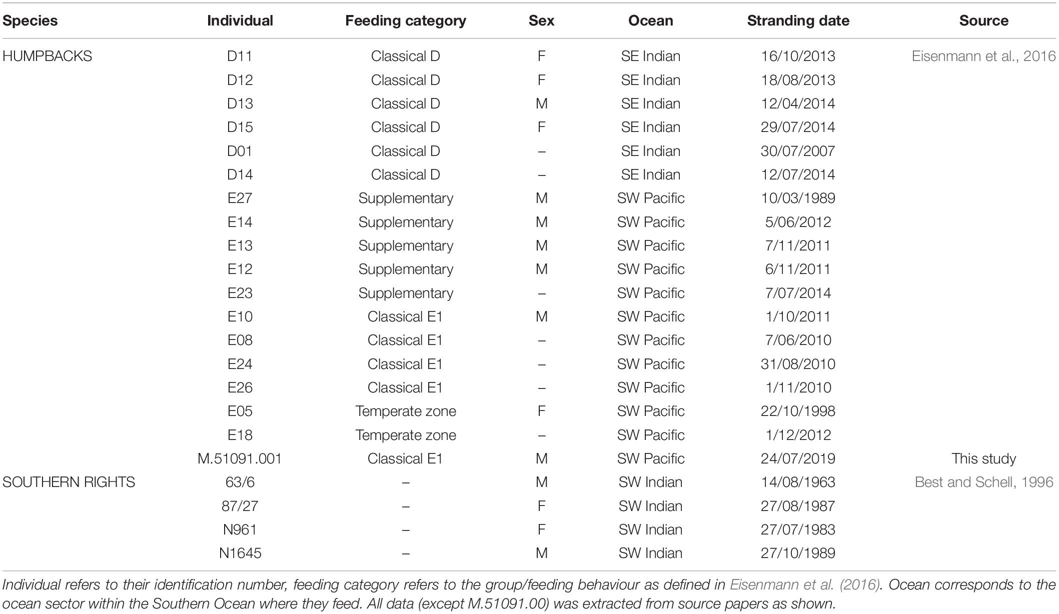
Table 1. Biological information for individuals within this study, and source identifying where data was extracted (all but one individual that was opportunistically sampled by the Australian Museum).

Additionally, we sampled a single baleen plate that was opportunistically collected from a dead adult male humpback stranded on the 24/7/2019 at Stockton beach, Newcastle, Australia and loaned to us for stable isotope analyses from the collection at the Australian Museum (individual identification: “M.51091.001”). This plate had been taken from between the middle to back of the whale’s mouth, representing the longest plates, i.e., to obtain the longest record. The plate was removed from within the gum to ensure the unerupted section beneath the gum was included.

Stable Isotope Analysis

The baleen plate was first cleaned with Milli-Q water, followed by a 2:1 chloroform:methanol solution using steel wool. This was repeated twice to ensure surface lipids and contaminants were removed before sampling. Using a Dremel engraving tool with a flexible shaft, approximately 0.5 mg of baleen powder was collected every 1 cm along the longitudinal growth axis, 0.5 cm from the outer edge, starting at the proximal end (most recent growth). Powdered samples were loaded into tin capsules and compressed airtight for processing and analysis using the Flash 2,000 organic elemental analyser, interfaced with a Delta V Advantage Isotope Ratio Mass Spectrometer via a ConFlo IV interface (Bioanalytical Mass Spectrometry Facility, Mark Wainwright Analytical Centre, UNSW Sydney). δ¹⁵N and δ¹³C values are expressed as a deviation from standards in parts per thousand (‰):

$\mathrm{\delta }X=\left[\left(\frac{Rsample}{Rstandard}\right)-1\right]\times \mathrm{\hspace{0.25em}1},000$

where X = ¹³C or ¹⁵N, R = the ratio of respective heavier and lighter stable isotopes of nitrogen (N¹⁵/N¹⁴) and carbon (C¹³/C¹²). Reference standards of nitrogen and carbon USGS40 and USGS41A were used to correct potential drift caused by the instrument prior to isotope abundance calculation. C:N ratios ranged from (3.4 ± 0.1) which were within the range of pure keratin (3.4 ± 0.5) (Hobson and Schell, 1998; Trueman et al., 2019).

Time Sectioning Baleen

To establish the time that the stable isotope values represent, we estimated the time over which the section of baleen grew. We used three values: (1) the baleen plate growth rate; (2) the date the baleen stopped growing (when the whale died); and (3) the interval between samples taken along the baleen plate.

We used baleen growth rates reported by Best and Schell (1996) for their southern right whale specimens and those reported by Eisenmann et al. (2016) for their humpback whale specimens with the exception of the Australian Museum collection specimen “M.51091.001” where we calculated the growth rate using the technique described by Eisenmann et al. (2016). This technique is based on the assumption that the oscillations in stable isotope values along the baleen plate reflect annual physiological changes as the whales move from feeding to fasting (Best and Schell, 1996; Eisenmann et al., 2016). Specifically, for the whales in this study lower δ¹⁵N values reflect times when the animal is feeding and higher δ¹⁵N values are associated with fasting during migration. Therefore, to calculate the growth rate of baleen the length between two adjacent δ¹⁵N minima were used to identify 1 year of growth. This is based on the assumption that baleen growth is linear and constant through time and between individuals of the same species, which may not always be true.

The stranding date (per individual) was used as the date when the baleen stopped growing. We assume that the baleen plates were collected from within the gum of the whale, meaning the entire plate (including the unerupted section containing the most recent growth) was included.

We calculated the number of days between each data point using the individual-specific growth rate and sampling interval (distance between each sampling point (cm)) then assigned a date to each point based on the cumulative days since the time of last known growth (stranding date) (see Supplementary Table 1 for functions). We assumed isotopic assimilation was constant in all animals despite potential differences in individual physiology, e.g., reproductive state, breeding condition, and fasting (Hobson et al., 1993; Lee et al., 2012; Clark et al., 2016). However, this study is the first step in investigating links between isotope values in baleen and climate cycles and how individual physiology impacts these relationships is the next step in this work.

Climate Data

El Niño-Southern Oscillation

ENSO is an important driver of climate in the Pacific Ocean, but its influence is broader across the Southern Hemisphere. We used the Southern Oscillation Index (SOI, as a measure for ENSO) which measures the pressure differences between Tahiti and Darwin, Australia and indicates the development and intensity of El Niño and La Niña events between 1876 and present. We extracted data from the Australian Bureau of Meteorology (BOM).¹ The BOM calculates the SOI using the Troup SOI method which is the standardised anomaly of the Mean Sea Level Pressure difference between Tahiti and Darwin (Troup, 1965) with multiplication by 10 used as a convention to quote a whole number that ranges between –35 and ∼ +35. The BOM specifies sustained negative SOI values below –7 typically indicate periods of El Niño, while sustained positive SOI values greater than +7 typically indicate La Niña events. Monthly SOI values were extracted for use in models with isotope data. Yearly averages were also calculated by taking the average of all monthly indices for each year of interest (SOI dataset available upon request).

Indian Ocean Dipole

The IOD is an important driver of climate in the Indian Ocean. We used the Dipole Mode Index (DMI) to identify the influence of the IOD. DMI is an indicator of the east-west temperature gradient, represented by anomalous sea surface temperatures (SST) along the western equatorial Indian Ocean and the southeastern equatorial Indian Ocean (Saji et al., 1999). We extracted DMI data from the National Oceanic and Atmospheric Administration (NOAA).² Monthly DMI values were extracted in the DMI: Standard PSL Format. Positive IOD events are represented by positive DMI values while negative IOD events are shown through negative DMI values (DMI dataset available upon request).

Southern Annular Mode

The SAM, also known as the Antarctic oscillation index (AAO), is a circumpolar climate driver in the Southern Ocean. It describes the north-south movement of the westerly wild belt that circulates Antarctica, thus dominating the mid-to-high-latitude regions of the Southern Hemisphere (Gong and Wang, 1999). We used AAO data extracted from the NOAA³ to identify the influence of SAM. Monthly mean AAO values were extracted from 1979 to 2021. The NOAA calculates monthly indices of SAM by projecting the monthly mean (700-hPa) height anomalies onto the leading Empirical Orthogonal Function mode. This is then normalised by the standard deviation of the monthly index over a base period from 1979 to 2000. Yearly averages were also calculated by taking the average of all monthly indices for each year. Isotope data for one of the southern right whales (individual “63/6”) was outside this time frame and therefore this individual was excluded from the SAM analysis (AAO dataset available upon request).

Statistical Analysis

There is large intraspecific variation in δ¹⁵N and δ¹³C values for both humpback and southern right whales, as shown by the high R² conditional values relative to R² marginal values. This, among other things may be due to individual whales feeding in different regions of the Southern Ocean or feeding on prey of different sizes or species. Alternatively, it may be due to shifts in the isotopic baseline in the ocean (McMahon et al., 2015) or multiple biochemical factors associated with or influenced by isotopic fractionation (Newsome et al., 2010). As a result of this intraspecific variation, we developed indices for δ¹⁵N and δ¹³C stable isotope values. These indices allowed us to determine the relative importance of data points and compare values among individuals. To do this we used individual-specific weighted averages for the stable isotope values of each whale, equalising the frequency of the values in the data set so that the final index values reflect the relative importance of each observation, placing individuals on the same scale. Firstly, individual-specific means of δ¹⁵N and δ¹³C values were calculated. Then, per individual, each isotope value along the baleen plate was subtracted from the individual-specific mean, resulting in a positive or negative variance from that mean. These values formed the nitrogen index (for δ¹⁵N values) and carbon index (for δ¹³C values):

$\mathrm{Nitrogen}\mathrm{index}=\mathrm{a}-((\mathrm{\Sigma }\mathrm{a})/\mathrm{N})$

Where within an individual whale’s baleen plate, a is the δ¹⁵N value at any position; Σa is the sum of all δ¹⁵N values; and N is the total number of δ¹⁵N observations.

$\mathrm{Carbon}\mathrm{index}=\mathrm{c}-((\mathrm{\Sigma }\mathrm{c})/\mathrm{N})$

Where within an individual whale’s baleen plate, c is the δ¹³C value at any position; Σc is the sum of all δ¹³C values; and N is the total number of δ¹³C observations.

Isotopic results are expressed as a ratio. To calculate weighted averages for ratios each value needs to be multiplied by their respective weight (i.e., by the denominator of the ratio). Here the assumption is that the values of the denominators across the samples were equal, which may not be true. The transformation of the original stable isotope values to our nitrogen and carbon index values means they are no longer stable isotope ratios as we traditionally know them, but values that reflect the relative importance of any data point within each whale’s series.

We did not adjust raw δ¹³C values in baleen to account for the Suess effect (Young et al., 2013). This was because we did not directly compare absolute δ¹³C values between years. Instead we compared the intra-individual variability using our aforementioned carbon index.

Linear mixed-effects models (LMM) were fitted using the lmer function (Bates et al., 2014) to determine the model of best fit. This approach assumes the relationship is strictly linear. Individual whale was included as a random effect across all models as there were multiple sequential samples taken from the baleen of each individual. Species were analysed separately to avoid comparisons between animals with different feeding and spatial patterns and humpbacks were analysed within their feeding group (E1 classical feeders: n = 5, data points = 208; E1 supplementary feeders: n = 5, data points = 122; E1 temperate feeders: n = 2, data points = 58; D classical feeders: n = 6, data points = 184). For both humpback and southern right whales monthly and yearly anomalies of ENSO, IOD and SAM were included as predictor variables alongside lags of 6 months and 1–4 years for IOD and SAM and 6 month and 1–7 years for ENSO. Lastly, nitrogen and carbon indices were included as the response variable in models with all environmental combinations, resulting in a total of 390 models. The Akaike Information Criterion (AIC) was used to select the most parsimonious models owing to model simplicity. Due to the theoretical problems associated with R² as outlined by Nakagawa and Schielzeth (2013), marginal and conditional R² values were initially reported, displaying the influence of fixed effects alone and combined with the random effects, respectively. However, after removing individual variation by establishing both indices, only R² marginal values were reported. R² marginal values were used to compare the models of best fit across these data sets of different sizes and to provide the absolute value for goodness-of-fit which cannot be provided by the aforementioned information criteria. This was done using the MuMIn package (Burnham and Anderson, 2002). All analyses were conducted in R (R Core Team, 2021).

Multicollinearity between stable isotope values and the climate predictors ENSO, SAM, and IOD was assessed using variance inflation factor (VIF) scores. The results indicated an absence in multicollinearity for humpbacks (1.1, 1.6, 1.4) and southern right whales (2.7, 1.1, 2.9) based on established criterion (Gareth et al., 2013). While the VIF of 2.6 and 2.9 are close to 3, when each climate driver was removed for testing it did not signify a correlation. Thus, all three climate predictors were kept within 390 models.

Results

Due to large individual variation in δ¹⁵N and δ¹³C values for humpback and southern right whales, all statistical analysis was done through indices to put individuals on the same scale, known as their nitrogen index and carbon index. We observed changes in stable isotope values within the baleen of both humpback and southern right whales alongside changes in climate cycles. Particularly, we found that humpback whales from the Southwest Pacific that primarily feed in the Southern Ocean show a positive (+) relationship between stable isotope values and ENSO/SAM with a 4-year lag. We observed enriched δ¹⁵N and δ¹³C values during + SAM and La Niña phases and depleted δ¹⁵N and δ¹³C values during negative (–) SAM and El Niño phases when lagged 4 years. On the other hand, Southern Ocean feeding humpback and southern rights in the Indian Ocean, show the opposite negative relationship with SAM at a lag period of 2–4-years, observing enriched δ¹⁵N and δ¹³C values during – SAM and depleted δ¹⁵N and δ¹³C during + SAM.

Southwest Pacific Ocean

Classical Southern Ocean Feeders of the E1 Breeding Stock

Humpback whales of the E1 breeding stock (Southwest Pacific) that predominately feed in the Southern Ocean (classical feeders), showed a positive relationship between both their nitrogen and carbon indices and changes in ENSO and SAM at 4-year lags. For their nitrogen index, we found higher δ¹⁵N values with less variation during La Niña periods with a monthly 4-year lag (p < 0.01; R²m = 0.04) (Figure 1), while there appears to be lower δ¹⁵N values with greater variation observed during El Niño periods. There was also a positive relationship between the carbon index and SAM anomalies at a yearly 4-year lag, whereby, higher δ¹³C values correlated with + SAM anomalies and lower δ¹³C values with—SAM anomalies (p < 0.01; R²m = 0.15) (Supplementary Figure 1). While there were other models of statistical significance, these models explained the most variance having the highest R²m and lowest AIC.

FIGURE 1

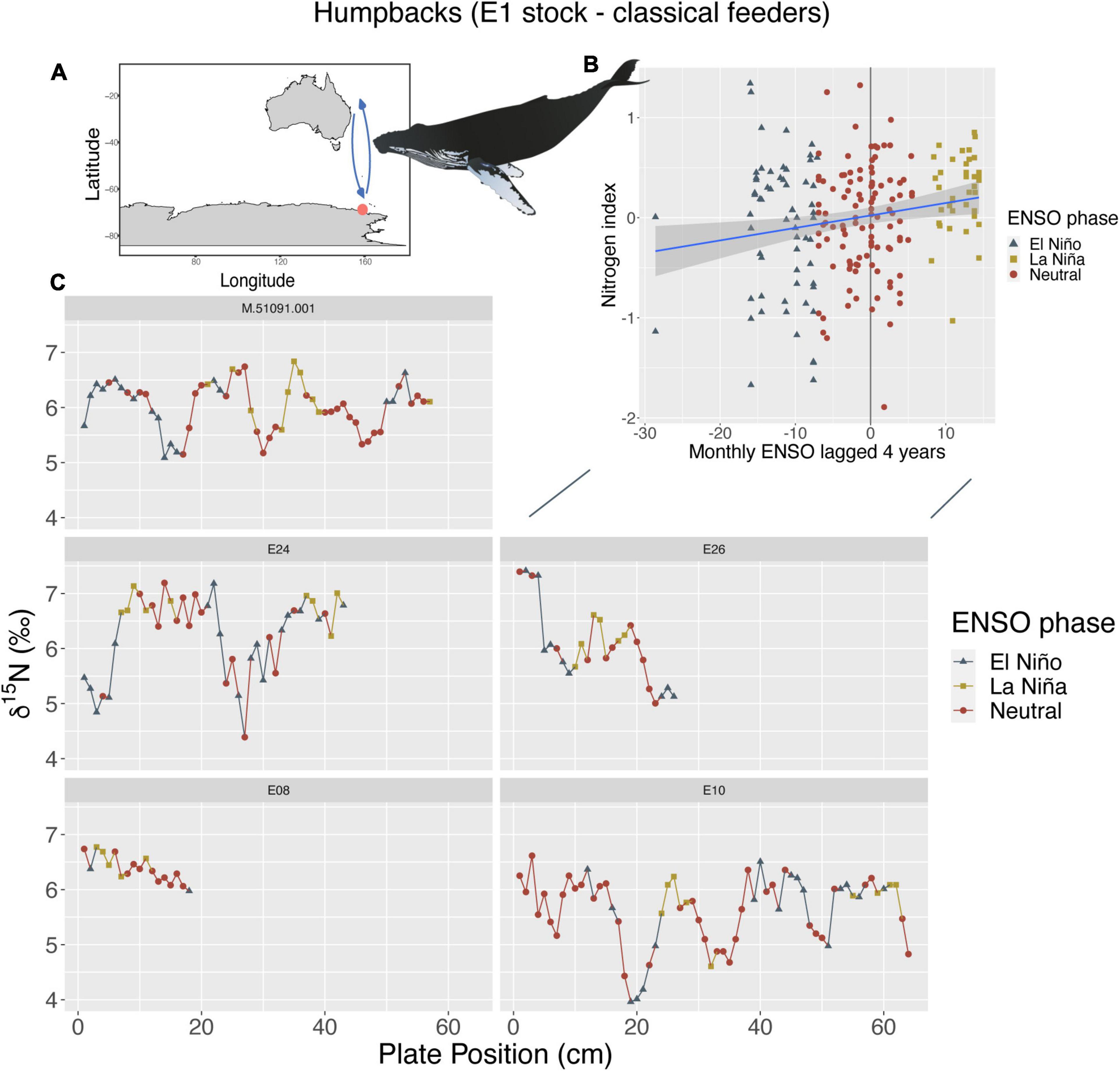
Figure 1. (A) Humpbacks from the E1 breeding stock (n = 5, sample points = 208) that primarily feed within the Southwest Pacific Ocean (known as classical feeders, orange circle = feeding location, arrows = migration route), show a positive linear relationship between their nitrogen index and ENSO (B) with a 4-year lag period (p < 0.01; R²m = 0.04). (C) Shows where these changes in ENSO phases occur along baleen and resulting stable isotope patterns of δ¹⁵N for each individual. Whale image attribution: Tracey Saxby, Integration and Application Network (ian.umces.edu/media-library).

Supplementary and Temperate Zone Feeders of the E1 Breeding Stock

Humpbacks from the E1 breeding stock that supplement their feeding outside of the Southern Ocean showed a positive relationship between their nitrogen index and yearly SAM anomalies with a zero-lag period (p < 0.01; R²m = 0.16). We found that higher δ¹⁵N values occur during + SAM and lower δ¹⁵N values toward—SAM phases (Figure 2). Their carbon index showed a negative relationship with yearly IOD anomalies at a 1-year lag (p < 0.01; R²m = 0.11), with higher δ¹³C values toward—IOD and lower δ¹³C values toward + IOD phases (Supplementary Figure 2). However, all humpbacks that supplemented their feeding mainly assimilated isotopic signals during times of positive IOD events, therefore visual trends across phases cannot accurately be seen.

FIGURE 2

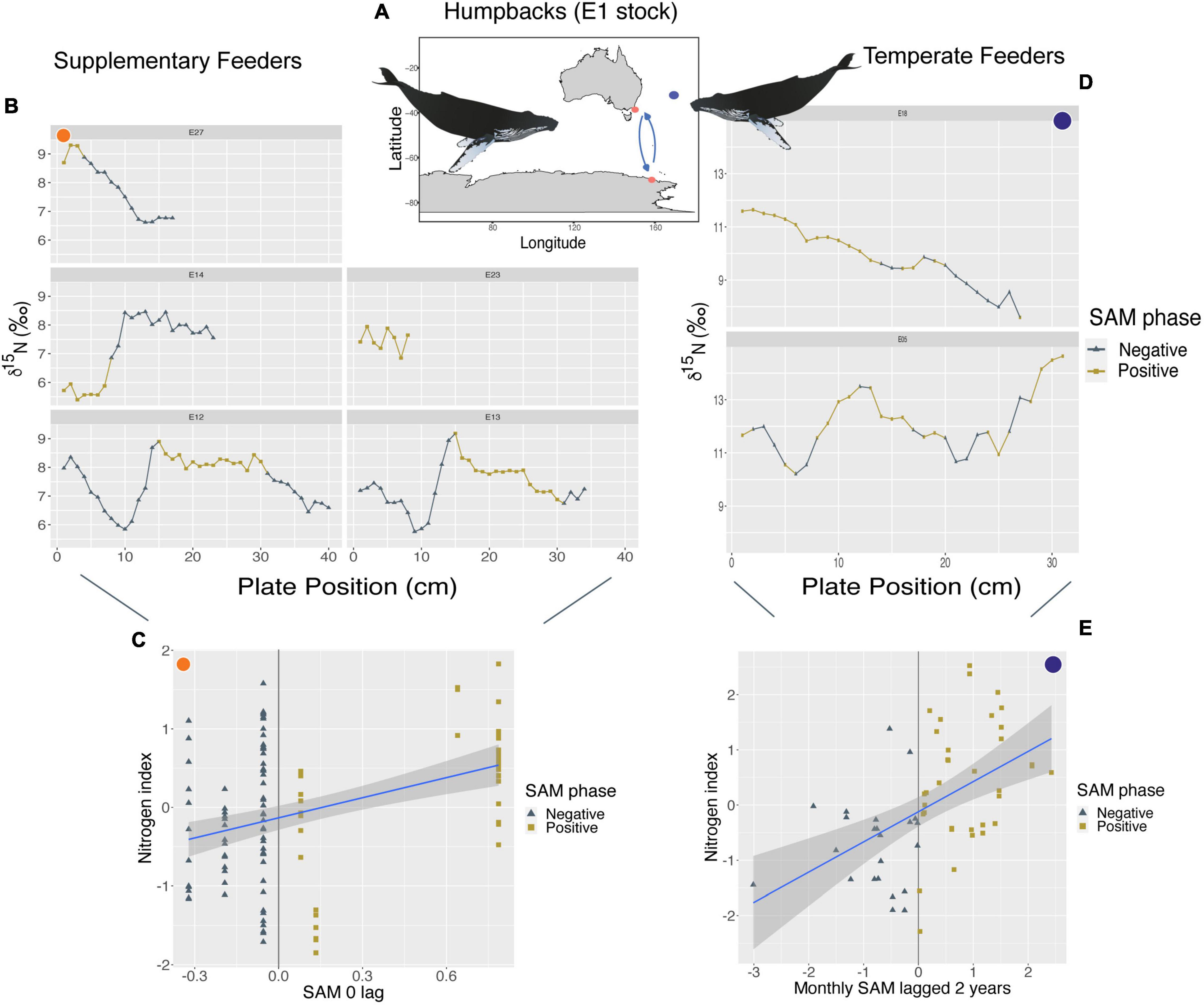
Figure 2. (A) Orange circles represent the approximate feeding locations of humpbacks from the E1 breeding stock (Southwest Pacific Ocean) that supplement their feeding in Australian waters (n = 5, sample points = 122). Purple circle represents an approximate location of humpbacks from the same breeding stock that remain in Australian waters year-round (known as temperate feeders, n = 2, sample points = 58). (C,E) Show a positive linear relationship between their nitrogen index and SAM, however, supplementary feeders (C) at a 0-year lag (p < 0.01; R²m = 0.16), and temperate feeders (E) at a monthly 2-year lag (p < 0.01; R²m = 0.25). (B,D) Show where these changes in SAM phases occur along baleen and resulting stable isotope patterns of δ¹⁵N of each individual. Whale image attribution: Tracey Saxby, Integration and Application Network (ian.umces.edu/media-library).

Humpback whales from the E1 breeding stock who remained in temperate regions year-round displayed variability in isotopic values alongside changes in SAM at 2- and 3-year lags. We found a positive relationship between their nitrogen index and monthly SAM anomalies at a 2-year lag (p < 0.01; R²m = 0.25), where enriched δ¹⁵N values occurred during + SAM and depleted δ¹⁵N values during –SAM (Figure 2). Their carbon index showed a negative relationship between δ¹³C values and yearly SAM anomalies at a 3-year lag (p < 0.01; R²m = 0.75), where enriched δ¹³C values were observed during -SAM and depleted δ¹³C values during + SAM phases (Supplementary Figure 3). However, this relationship is only driven by 2 individuals (58 samples) and so we caution that it represents possible trends.

South Indian Ocean

Humpback Whales (D Breeding Stock) and Southern Right Whales (South African Stock) in the Indian Ocean

Both the humpback whales of the D breeding stock (Southeast Indian Ocean), and the southern right whales of the South African stock (Southwest Indian Ocean) feed predominantly within the Indian Ocean sector of the Southern Ocean and show the same negative relationship between nitrogen indices within baleen and changes in SAM. While the nitrogen index for D stock humpback whales was primarily influenced by monthly SAM anomalies at a 2-year lag (p < 0.01; R²m = 0.04), the nitrogen index of southern right whales was linked to yearly SAM anomalies at a 4-year lag (p < 0.05; R²m = 0.04). Despite the different time lags, both show higher δ¹⁵N values during—SAM phases and lower δ¹⁵N values during times of + SAM when lagged their respective years (Figure 3). δ¹⁵N values for D stock humpbacks also show a positive relationship with monthly IOD anomalies at a 2-year lag (p < 0.01; R²m = 0.04), with enriched δ¹⁵N values during + IOD and lower δ¹⁵N values during—IOD when lagged 2 years.

FIGURE 3

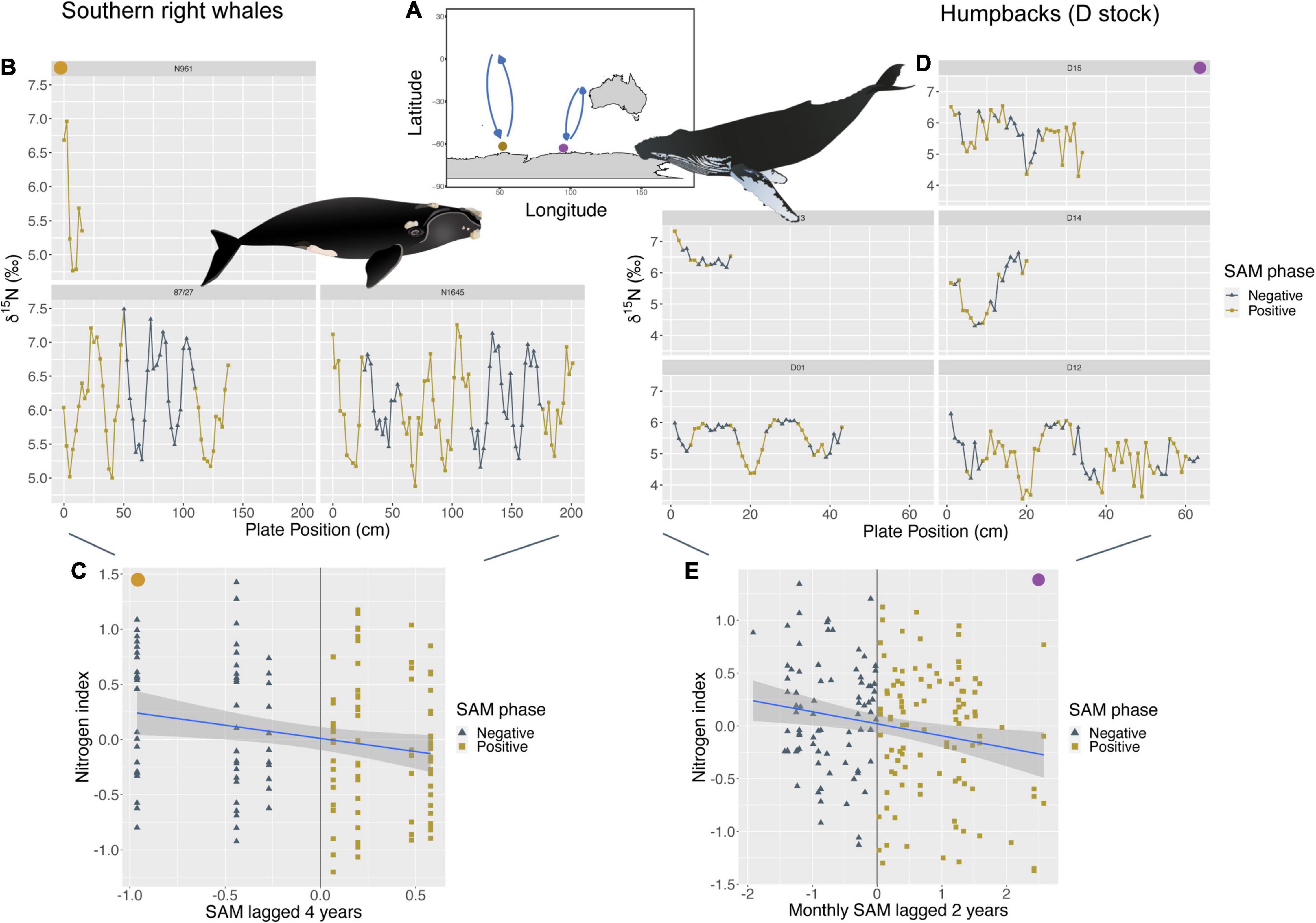
Figure 3. (A) The brown circle represents an approximate feeding location of southern right whales (SRW) from the South African population (Southwest Indian Ocean, n = 3, sample points = 144). While the light purple circle represents an approximate feeding location for humpbacks from the D breeding stock (Southeast Indian Ocean, n = 6, sample points = 184). (C,E) Show a negative linear relationship between their nitrogen index and SAM, however, SRW (C) at a 4-year lag (p < 0.05; R²m = 0.04) and D humpbacks (E) at a monthly 2-year lag (p < 0.01; R²m = 0.04). (B,D) Show where these changes in SAM phases occur along baleen and resulting stable isotope patterns of δ¹⁵N for each individual. Individual “D11” was removed from the image based on having a short baleen length. Humpback whale image attribution: Tracey Saxby, Integration and Application Network (ian.umces.edu/media-library). SRW image attribution: Jamie Testa, Integration and Application Network (ian.umces.edu/media-library).

We also found links between SAM and the carbon index of humpback and southern right whales within the South Indian Ocean. Specifically, both had a negative relationship between their carbon index and SAM, with humpback values driven by monthly SAM anomalies at a 3-year lag (p < 0.01; R²m = 0.07) and southern right whale values driven by monthly SAM anomalies at a 4-year lag (p < 0.01; R²m = 0.11). For both species within the Indian Ocean, we observed higher δ¹³C values during-SAM and lower δ¹³C values during + SAM for both lag periods (Supplementary Figure 4). However, only ∼2 southern right whales were available for analysis with SAM; therefore, more data is needed to confirm these relationships.

Discussion

We show that for Southern Ocean feeding humpback and southern right whales, variation in baleen stable isotope values correlates with changes in large-scale climate cycles and that these relationships differ depending on the region in which individuals feed (Figure 4). For whales that feed predominantly in the Southwest Pacific, there is a positive relationship between both nitrogen and carbon stable isotope values with ENSO and SAM cycles when lagged 4 years. On the other hand, whales that feed predominantly in the Southeast and Southwest Indian Ocean show a negative relationship between nitrogen and carbon stable isotope values with SAM lagged 2–4years. The variation we observed in the isotopic values of whale baleen may reflect a shift in the resources available to individuals (as they feed on different prey types) and/or a change in isotopic baseline values as a response to variation during different environmental conditions.

FIGURE 4

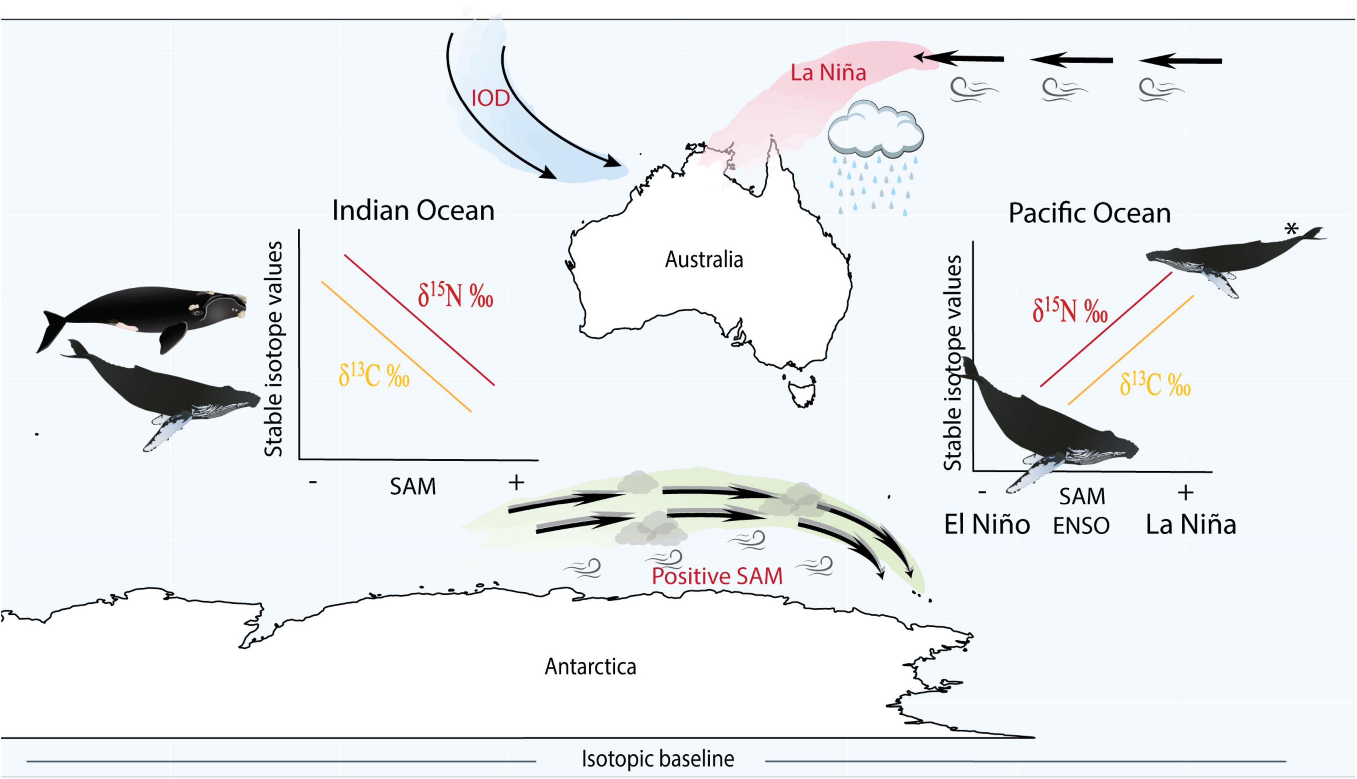
Figure 4. Schematic figure illustrating the main findings from the study and the positioning of climate cycles. La Niña (a phase of ENSO) corresponds to warmer and increased wet conditions in the west Pacific Ocean, while positive SAM (known to correspond to La Niña phases of ENSO) also drives an increase in storm conditions, however, has a stronger influence over the Southern Ocean. IOD is more prominent in the Indian Ocean and positive and negative phases are more complicated and not strictly in phase with either ENSO or SAM, making it difficult to compare with these climate cycles. Within the Pacific Ocean, we found that humpback whales displayed enriched nitrogen and carbon stable isotope values during positive SAM and La Niña periods (potentially reflecting poor feeding conditions) and depleted stable isotope values during negative SAM and El Niño phases. In the Indian Ocean we found the opposite trend, where humpback and southern right whales exhibited depleted nitrogen and carbon stable isotope values during positive SAM (potentially reflecting improved feeding conditions) and enriched isotope values during negative SAM. *In the Pacific Ocean during La Niña/positive SAM, whales from the same population were found to be in a lean body condition due to reduced sea ice concentration and resource availability (Bengtson Nash et al., 2018). However, such information is unavailable for whales in the Indian Ocean. Our interpretations assume variation in isotope values reflect changes in resource availability rather than variation in baseline isotope values.

We suggest that the spatial and temporal variation in ENSO and SAM (e.g., a positive SAM/La Niña phase may be beneficial in one region while not in another) as well as different lag periods (e.g., potentially the offset in SAM cycle timings within the Southern Ocean) could be reflected in the stable isotope values in baleen. However, there is little direct data on resource availability in regions where these whales are known to feed. Finally, our results demonstrate that climate cycles could be a source of isotopic variation, contributing to our understanding in interpreting isotopic patterns in baleen.

Southwest Pacific Ocean

Humpback Whales—Classical Southern Ocean Feeders of the E1 Breeding Stock

For humpbacks from the Southwest Pacific that primarily feed within the Southern Ocean, the climate cycles ENSO and SAM were positively associated with variation in nitrogen and carbon stable isotope values in baleen when lagged 4 years. We also found the same positive relationship between the stable isotope values and shorter lags in ENSO (6-month) and SAM (zero-lag) to be statistically significant. Stable isotope values were enriched and less varied during and 4 years following La Niña and positive SAM events but depleted and more varied during and 4 years following El Niño and negative SAM events. It is possible that the short and long-term lags reflect reoccurring cycles (4 years apart) of either ENSO (La Niña/El Niño) or SAM (positive/negative). Specifically, if similar anomalies in both ENSO and SAM occurred 4 years apart during the time baleen grew, isotopic values at short and long-term lags may reflect similar responses to resource availability and/or isotopic baseline changes associated with the reoccurring phase of either ENSO or SAM. These links between climatic conditions and isotopic variability may reflect different relationships. Firstly, changes in isotopic variability may imply that there has been a direct impact upon the whale’s feeding opportunities due to certain climatic conditions. Alternatively, there may have been a shift in the isotopic values at the base of the food chain (shifting baselines) rather than a true change in prey availability.

If these climate cycles do directly impact on resource availability, it may be possible that enriched and less variable stable isotope values in baleen during and 4 years following La Niña and positive SAM phases indicate that the whales experience less favourable feeding opportunities and/or longer fasting periods during these times. On the other hand, lower and more varied stable isotope values during and 4 years following El Niño and negative SAM events could suggest better feeding opportunities. Eisenmann et al. (2016) suggest that times of enriched nitrogen stable isotope values along baleen oscillations represent periods of fasting for this population, while slightly elevated carbon values coincide with times the whales were in Australian waters. Furthermore, they show that lower nitrogen stable isotope values predict times when the whales were feeding in the Southern Ocean, matched to lower carbon values within the Antarctic range (Eisenmann et al., 2016).

Within the Western Antarctic Peninsula, there is a reduction in sea ice duration following periods of positive SAM and La Niña phases (Stammerjohn et al., 2008). Furthermore, in the same region there is a reduction in krill recruitment following positive SAM events (Atkinson et al., 2019), which is said to be a result of reduced sea ice conditions that favour the survival of krill larvae (Siegel and Loeb, 1995; Quetin et al., 2007; Saba et al., 2014; Atkinson et al., 2019). Within the Pacific Ocean sector of the Southern Ocean, Bengtson Nash et al. (2018) showed that during La Niña and positive SAM events there was a similar trend between sea ice concentration and krill availability. Using the same breeding population, they also showed (via adiposity markers) that during these times of La Niña and positive SAM events, the southwestern Pacific humpbacks were in a lean body condition which they proposed was due to the reduced krill availability because of less sea ice. Similarly, in this study we infer that during positive SAM and La Niña periods, whales experience enhanced fasting seen through consistently enriched isotopic values in their baleen. Furthermore, the opposite occurs during negative SAM and El Niño phases, where there are signs of enhanced krill recruitment along the Western Antarctic Peninsula due to enhanced sea ice conditions favouring the survival of krill larvae (Siegel and Loeb, 1995; Quetin et al., 2007; Saba et al., 2014; Atkinson et al., 2019). The 4-year lag may alternatively represent a biological lag and/or cycle in krill development. It takes Antarctic krill approximately 3 years to develop into mature adults (Siegel, 1987), therefore the link seen between ENSO, SAM, and isotopic values in baleen may reflect changes in krill abundance according to their developmental stage. However, more research is required to confirm this link as there is no available krill data from the area in which these whales feed.

For the southwestern Pacific humpbacks, variability in isotope values is linked to two different climate cycles, where nitrogen stable isotope values are linked to ENSO and carbon values are linked to SAM. However, given the correlated nature of ENSO and SAM (particularly La Niña/positive SAM and El Niño/negative SAM; Fogt and Bromwich, 2006; Stammerjohn et al., 2008), it appears the relationship between nitrogen and ENSO and carbon and SAM may represent a similar 4-year signal. Within the Pacific Ocean, ENSO and SAM may modulate one another (Simmonds and King, 2004; Kohyama and Hartmann, 2016), potentially explaining why we see the positive influence of both ENSO and SAM on baleen isotope values for the southwestern Pacific feeding humpback whales.

La Niña events occurred more frequently among the dataset for the classical feeders, especially in the year prior to stranding. Based on the link we found between enriched and less varied nitrogen stable isotopes and La Niña events, we suggest that reoccurring La Niña phases could contribute to the likelihood of individual whales stranding (i.e., the source of baleen data used in this study). While we were limited by sample size and unable to statistically test this, Meynecke and Meager (2016) show a positive relationship between La Niña events also lagged 4 years and increased stranding occurrences in Queensland, Australia. This is supported further by Bengtson Nash et al. (2018) showing that humpbacks tend to be leaner and in poorer body condition during La Niña times. Therefore, there is growing evidence to suggest that, during La Niña years, humpback whales that feed in the Southwest Pacific suffer reduced feeding success, resulting in whales having a leaner body condition (Bengtson Nash et al., 2018) and thus a higher chance of stranding (Meynecke and Meager, 2016). Under scenarios predicting an increase in La Niña intensity (Cai et al., 2015), more research is needed to understand this potential link between resource availability, body condition and stranding potential for humpback whales of the E1 breeding stock.

Alternatively, the link we found between baleen isotopic variability and climatic cycles may be due to changes in the isotopic values at the base of the food web during different phases of ENSO and SAM. Baseline isotopic values of both nitrogen and carbon fluctuate seasonally, as well as spatially across the Southern Ocean (St John Glew et al., 2021). Therefore, this could mean that the observed enriched and depleted baleen stable isotope values of nitrogen and carbon (relative to other years) simply represents a baseline isotopic shift rather than the whales feeding on different prey or the same prey, but of different sizes. However, as we analysed the variability in isotope values within an individual via nitrogen and carbon indices rather than comparing the absolute nitrogen or carbon stable isotope values across whales, the variation shown here is less likely to be purely an artifact of a shifting baseline, although this cannot be discounted.

Southwestern Pacific Humpback Whales—Supplementary and Temperate Feeders of the E1 Breeding Stock

Humpback whales from the same southwestern Pacific population (E1) can use alternate strategies and deviate from classical Southern Ocean feeding, i.e., supplement their feeding or stay in Oceania year-round (Eisenmann et al., 2016). Much less is known about humpback whales that supplement their feeding during their annual migration, as well as individuals that refrain from migration and remain at lower latitudes year-round. Therefore, the feeding behaviour of these groups is more difficult to interpret as they can feed across multiple regions with different isotopic baselines and as a result are influenced by Southern Ocean and temperate systems.

Whales that feed both in the Southern Ocean and temperate waters (known as supplementary feeders) show the same positive relationship between their nitrogen stable isotope values and SAM to the classical feeders with elevated nitrogen values during positive SAM and lower values during negative SAM, however, without any lagged effect. We suggest like the classical feeders, this may signify either changes in feeding patterns or isotopic baseline shifts during these different environmental conditions. For supplementary feeders, prolonged elevated nitrogen stable isotopes during positive SAM correspond to sustained low carbon values within the Antarctic range. If the isotopic variation reflects changes in feeding patterns, the sustained and elevated nitrogen values (seen alongside Antarctic carbon values) may either show prolonged times of fasting or feeding at higher trophic levels within the Southern Ocean. In the first instance, like the classical feeders of the same E1 breeding stock, it is possible that elevated nitrogen values may reflect a reduction in resource availability (e.g., krill) associated with a reduction in sea ice during positive SAM/La Niña phases (Bengtson Nash et al., 2018) and thus increased fasting. Secondly, the signal may reflect feeding at higher trophic levels within the Southern Ocean (Eisenmann et al., 2016). If the latter were true, it is possible these whales may switch to other food items within the Southern Ocean in the absence of abundant krill. Alternatively, like the classical feeders, isotopic variability may simply be reflecting baseline changes during these times. These prolonged isotopic signals are ended by the whales supplementing their feeding in Australian waters (as seen by higher nitrogen and carbon stable isotope values within the Australian range). Evidently, we showed that two individuals (E12 and E13) tended to supplement their feeding after a prolonged positive SAM event. We suggest it is possible that whales within this study either supplement their feeding due to a reduction in available resources within the Southwest Pacific Ocean during these times or as a result of increased productivity in temperate waters. Nevertheless, more data from whales that supplement their feeding as well as the influence of climate cycles in temperate waters is needed to explore this theory.

While supplementary feeders may show similarities in their relationship between stable isotope values and SAM to classical feeders, their nitrogen values are not impacted by a lag period as seen in the classical feeders (4-year lag). This may suggest individuals choose to supplement their feeding based on environmental conditions at that time. Alternatively, Australian krill (Nyctiphanes australia) have shorter life cycles and are unlikely to live longer than 1 year (Ritz and Hosie, 1982) and therefore supplementary feeders may not be influenced by the biological lags in growth in the larger, longer-lived Antarctic krill. We also note that this data may be restricted in showing longer interannual trends as supplementary and temperate feeders within this study have shorter baleen lengths (and thus less assimilated long-term data).

There are many possible reasons behind why whales may supplement their feeding, one being due to environmental conditions that favour higher productivity in feeding hotspots (e.g., Eden) in the Tasman Sea off eastern Australia (Stamation et al., 2007). Humpback “super-groups” from the same E1 breeding stock have been documented feeding off Southeast Australia (Pirotta et al., 2021). Super-group formation has been linked to phytoplankton blooms 1 month prior as well as reduced outward transport favouring an increase in humpback whale prey in coastal waters, as found in Southern Benguela (Dey et al., 2021). E1 humpbacks are known to supplement their feeding anywhere between Eden, NSW, all the way down through the Bass Strait, Tasmania, and New Zealand, as shown through satellite tracking of the same population (Andrews-Goff et al., 2018). This could explain the relationship of IOD on their carbon stable isotope values as the influence of IOD is mostly seen across the Indian Ocean and southern Australia (Saji et al., 1999) where they may supplement their feeding. However, little is known about the influence of IOD within the regions where these whales feed. Secondly, all assimilated isotopic data collected from supplementary feeders occurred mostly during positive IOD phases; therefore, we suggest while a negative relationship with IOD may be occurring, more data from negative IOD alongside research focusing on supplementary feeders and environmental conditions are needed to understand this link and alternate strategy.

For whales who remain in Oceania year-round (known as temperate feeders), their continued presence and feeding in temperate waters may be driven by either poor Southern Ocean conditions or sustained localised productivity within temperate Tasman Sea waters. However, for temperate feeders, only two individuals were available and therefore we are not able to make assumptions on potential relationships. Interestingly, most whales that supplement their feeding in temperate waters appear to be males, however, more individuals of known sex are needed to explore the influence of sex differences among alternative feeding strategies.

South Indian Ocean

Humpbacks of the D Breeding Stock and the Southern Right Whales of the South African Stock

The Indian Ocean humpback (Southeast Indian) and southern right whales (Southwest Indian) that predominantly feed within the Southern Ocean show similar relationships between the variability of stable isotope values in their baleen and SAM, despite their different locations within the Indian Ocean. During positive SAM, both populations show an increase in low nitrogen and carbon stable isotope values, though with different lagged periods (humpbacks at monthly lags of 2 and 3 years, respectively, and southern rights at both yearly and monthly 4-year lags, respectively). According to both studies where the data was extracted from, low nitrogen and carbon stable isotope values reflect feeding signals in Antarctic regions (Best and Schell, 1996; Eisenmann et al., 2016). Therefore, unlike southwestern Pacific humpbacks (E1 classical feeders) who show signs of enriched nitrogen and carbon stable isotope values during positive SAM/La Niña periods (and potentially experience poor feeding conditions during summer), whales that feed within the South Indian Ocean show depleted isotope values during positive SAM phases (and potentially experience greater feeding opportunities).

Within the South Indian Ocean the opposite trend in sea ice extent occurs during positive SAM, where, unlike the Southwest Pacific Ocean sector showing sea ice decreases during positive SAM and La Niña events (Bengtson Nash et al., 2018), there is greater sea ice extent during positive SAM (as well as La Niña periods) (Kohyama and Hartmann, 2016). This was also shown through intense negative SST anomalies associated with positive SAM in the Indian Ocean, while negative SAM events were associated with positive SST anomalies (Sabu et al., 2020). Therefore, if the isotopic variability reflects changes in feeding success, it may be possible whales within the South Indian Ocean experience better feeding opportunities (i.e., better krill recruitment) during these times as seen through an increase in low nitrogen and carbon stable isotope values. Similarly, like the southwestern Pacific humpbacks, while we analysed isotopic variability via indices rather than absolute values of stable isotopes, the impact of shifting isotopic baselines may still impact these conclusions.

Humpbacks from the D breeding stock also show a positive relationship between nitrogen stable isotope values in baleen and changes in monthly IOD when lagged 2 years, displaying lower nitrogen stable isotope values during negative IOD phases, with higher values during positive IOD phases. Within the South Indian Ocean, the impact of IOD on this population is unclear. Unlike the southwestern Pacific humpbacks (E1 stock), where feeding grounds are known from satellite tracked individuals (Andrews-Goff et al., 2018), there is less information available for humpbacks as well as the influence of IOD on resource availability within the Southeast Indian Ocean. Therefore, it is difficult to interpret this relationship, especially when isotopic data is from predominantly positive IOD phases and lacks isotope values during negative IOD periods.

The 4-year lag for southern right whales may reflect the biological timing in longer-lived Antarctic krill development and/or growth (as discussed for the southwestern Pacific classical feeders) or the frequency in reoccurring phases of SAM captured in these individuals. The 2- and 3-year lags for the humpback whales could also reflect biological lags and/or phase reoccurrences, however, the slightly shorter lag periods may be due to their different feeding location within the Southern Ocean. Thus, lags between stable isotope values and climate anomalies may differ depending on the feeding location within the Southern Ocean due to the temporal and spatial variability in climate cycles.

Indian Ocean humpbacks (D stock) show less variation in feeding strategies than the southwestern Pacific humpbacks (E1 stock) (Eisenmann et al., 2016). Unlike the humpbacks from the Indian Ocean, humpbacks from the Southwest Pacific, may be able to supplement their feeding on reliable spring blooms each year in the Tasman Sea. For example, the southeastern NSW coast is subject to high productivity in spring due to warmer East Australian Current water overlaying uplifted sub-Antarctic waters high in nutrients (Hallegraeff and Jeffrey, 1993; Bax et al., 2001). However, in the Southeast Indian Ocean, there has been comparably little documentation of supplementary behaviour. Therefore, during times of increased productivity within their Southern Ocean feeding grounds, humpbacks from the Indian Ocean may decide to prioritise feeding and spend more time at higher latitudes as a result. This is potentially what we see in this population through greater variability in their nitrogen and carbon stable isotope values during positive SAM events.

If variability among isotope values reflect changes in feeding success in southern right whales (and humpback individual D12), they did not appear to be as adversely impacted by fasting during positive SAM events, as seen through lower peaks in nitrogen isotope values. This further suggests they may experience better feeding opportunities during these times. While limited by sample size and the availability of isotopic baseline data within the Indian Ocean, an increase in feeding success may allow the whales to withstand the impacts of fasting better (meaning less enrichment of nitrogen stable isotopes). However, more research tracking these populations as well as on the effect of climate cycles within the area is necessary to understand what these relationships mean.

Baleen Oscillation Patterns

In this study, we show that some of the isotopic variability in baleen oscillations is related to changes in climate cycles and thus may assist in the interpretation of complex stable isotope patterns in baleen. We recommend analysing the influence of climate on stable isotope patterns across multiple individuals and species through an index. This technique allowed us to compare changes and variability in stable isotopes (e.g., feeding patterns) across individuals that may be feeding on different food items in different regions. Also, this allowed us to compare variability on the same scale and avoid direct comparisons of absolute values that may be influenced by the known Suess effect (Young et al., 2013). Furthermore, the time stamp attribution allowed us to assign each section of baleen to a date for comparison with climate anomalies. However, this assumed that baleen growth rate is linear and that all baleen plates were collected in a similar manner (e.g., including the unerupted section within the gum) for accurate time attribution. We acknowledge the R² values within this study are low, however, we suggest that the nature of our data, being patchy between years (from different stranding dates), as well as our limited sample size may result in weakening potential relationships. Data from more adult individuals to fill these sampling gaps may assist in establishing stronger trends. This is the first step in defining what links exist between isotopic signatures in baleen and climate, however, more research is needed to understand how these links are impacted by baseline changes as well as the whale’s reproductive state, condition and fasting behaviour. There is large intraspecific and intra-individual variation in oscillation cycles lengths (which are assumed to be annual), however, the data was not at hand to examine this here. Therefore, our next step will be addressing this variation seen in cycle lengths in terms of environmental and/or physiological drivers. Future work on how isotopic baselines shift with large-scale climate cycles on an interannual scale would be beneficial to understand what long-term isotopic values are responding to in marine predators.

Conclusion

We show that a relationship exists between the nitrogen and carbon stable isotope values in whale baleen and changes in climate cycles. In addition, we show that these relationships differ depending on the whale’s feeding location within the Southern Ocean. We propose this variability in isotope values may reflect changes in resource availability driven by these climate cycles (regardless of which ocean sector they reside in), however, further research is needed to understand how a whale’s physiology, reproductive state, and changes in the isotopic baseline may contribute to these relationships. This research contributes to our understanding and interpretation of complicated stable isotope oscillation patterns along baleen plates of whales. Understanding long-term patterns will become extremely important within a changing climate, considering how the frequency and intensity of climate cycles are predicted to change. However, given the complexity of interpreting bulk stable isotopes across multiple isoscapes, particularly within rapidly changing environments, challenges remain in defining links between isotope signatures in whale baleen and climate/environmental cycles. Considering the temporal and spatial variability across the Southern Ocean in terms of climate cycles and resulting resource availability, we recommend future research focus on multiple species across different ocean sectors to understand broad scale responses to environmental change.

Data Availability Statement

The raw data supporting the conclusions of this article will be made available by the authors, without undue reservation.

Ethics Statement

Ethical review and approval was not required for the animal study because ethics for this study was not required, as data was sourced from available online literature or specimens for analysis provided on loan to us from the Australian Museum.

Author Contributions

AD and TR conceived the ideas, designed the project, and interpreted the results and their significance. AD extracted data, conducted lab work and isotopic analysis, and statistical analysis. Both authors contributed critically to the drafts and gave final approval for publication.

Funding

This work was funded to TR from Scott Foundation under grant RG161708.

Conflict of Interest

The authors declare that the research was conducted in the absence of any commercial or financial relationships that could be construed as a potential conflict of interest.

Publisher’s Note

All claims expressed in this article are solely those of the authors and do not necessarily represent those of their affiliated organizations, or those of the publisher, the editors and the reviewers. Any product that may be evaluated in this article, or claim that may be made by its manufacturer, is not guaranteed or endorsed by the publisher.

Acknowledgments

We would like to thank Gary Truong for his assistance with coding for this project, particularly for the time stamp attribution. We would also like the thank Junlin Lyra Huang for her advice and assistance with aspects of coding. We thank the mammal lab at UNSW, in particular Anna Lewis for providing comments on draft manuscripts. We would like to thank Leanne and Lewis at the Bioanalytical Mass Spectrometry Facility at UNSW for their assistance in running a small number of samples for this study. We also thank the Australian Museum, in particular Sandy Ingleby (Collection Manager, Mammalogy) for the loan and access of opportunistic baleen for this research. We thank NSW National Parks and Wildlife Service staff in assisting with baleen collection on site at Newcastle. We also thank Tracey Saxby and Jamie Testa (Integration and Application Network) for the use of whale images on figures as referenced within figure captions.

Supplementary Material

The Supplementary Material for this article can be found online at: https://www.frontiersin.org/articles/10.3389/fmars.2022.832075/full#supplementary-material

Footnotes

1. ^ http://www.bom.gov.au/climate/enso/soi_monthly.txt
2. ^ https://psl.noaa.gov/gcos_wgsp/Timeseries/Data/dmi.had.long.data
3. ^ https://www.cpc.ncep.noaa.gov/products/precip/CWlink/daily_ao_index/aao/monthly.aao.index.b79.current.ascii

References

Aguilar, A., Gimenez, J., Gomez-Campos, E., Cardona, L., and Borrell, A. (2014). delta15N value does not reflect fasting in mysticetes. PLoS One 9:e92288. doi: 10.1371/journal.pone.0092288

PubMed Abstract | CrossRef Full Text | Google Scholar

Andrews-Goff, V., Bestley, S., Gales, N., Laverick, S., Paton, D., Polanowski, A., et al. (2018). Humpback whale migrations to Antarctic summer foraging grounds through the southwest Pacific Ocean. Sci. Rep. 8:12333.

Google Scholar

Arrigo, K. R., and van Dijken, G. L. (2004). Annual changes in sea-ice, chlorophyll a, and primary production in the Ross Sea, Antarctica. Deep Sea Res. Part II Top. Stud. Oceanogr. 51, 117–138. doi: 10.1016/j.dsr2.2003.04.003

CrossRef Full Text | Google Scholar

Atkinson, A., Hill, S. L., Pakhomov, E. A., Siegel, V., Reiss, C. S., Loeb, V. J., et al. (2019). Krill (Euphausia superba) distribution contracts southward during rapid regional warming. Nat. Clim. Change 9, 142–147. doi: 10.1038/s41558-018-0370-z

CrossRef Full Text | Google Scholar

Atkinson, A., Siegel, V., Pakhomov, E., and Rothery, P. (2004). Long-term decline in krill stock and increase in salps within the Southern Ocean. Nature 432, 100–103. doi: 10.1038/nature02996

PubMed Abstract | CrossRef Full Text | Google Scholar

Bates, D., Mächler, M., Bolker, B., and Walker, S. (2014). Fitting linear mixed-effects models using lme4. arXiv [preprint]. arXiv:1406.5823.

Google Scholar

Bax, N. J., Burford, M., Clementson, L., and Davenport, S. (2001). Phytoplankton blooms and production sources on the south-east Australian continental shelf. Mar. Freshw. Res. 52, 451–462. doi: 10.1071/MF00001

CrossRef Full Text | Google Scholar

Bengtson Nash, S. M., Castrillon, J., Eisenmann, P., Fry, B., Shuker, J. D., Cropp, R. A., et al. (2018). Signals from the south; humpback whales carry messages of Antarctic sea-ice ecosystem variability. Glob. Change Biol. 24, 1500–1510. doi: 10.1111/gcb.14035

PubMed Abstract | CrossRef Full Text | Google Scholar

Bentaleb, I., Martin, C., Vrac, M., Mate, B., Mayzaud, P., Siret, D., et al. (2011). Foraging ecology of Mediterranean fin whales in a changing environment elucidated by satellite tracking and baleen plate stable isotopes. Mar. Ecol. Prog. Ser. 438, 285–302. doi: 10.3354/meps09269

CrossRef Full Text | Google Scholar

Best, P., and Schell, D. (1996). Stable isotopes in southern right whale (Eubalaena australis) baleen as indicators of seasonal movements, feeding and growth. Mar. Biol. 124, 483–494. doi: 10.1007/BF00351030

CrossRef Full Text | Google Scholar

Borrell, A., Gómez-Campos, E., and Aguilar, A. (2016). Influence of reproduction on stable-isotope ratios: nitrogen and carbon isotope discrimination between mothers, fetuses, and milk in the fin whale, a capital breeder. Physiol. Biochem. Zool. 89, 41–50. doi: 10.1086/684632

PubMed Abstract | CrossRef Full Text | Google Scholar

Burnham, K. P., and Anderson, D. R. (2002). Model Selection and Multimodel Inference. A Practical Information-Theoretic Approach, 2nd Edn. New York, NY: Springer.

Google Scholar

Busquets-Vass, G., Newsome, S. D., Calambokidis, J., Serra-Valente, G., Jacobsen, J. K., Aguiniga-Garcia, S., et al. (2017). Estimating blue whale skin isotopic incorporation rates and baleen growth rates: implications for assessing diet and movement patterns in mysticetes. PLoS One 12:e0177880. doi: 10.1371/journal.pone.0177880

PubMed Abstract | CrossRef Full Text | Google Scholar

Cai, W., Borlace, S., Lengaigne, M., Van Rensch, P., Collins, M., Vecchi, G., et al. (2014). Increasing frequency of extreme El Niño events due to greenhouse warming. Nat. Clim. Change 4, 111–116. doi: 10.1038/nclimate2100

CrossRef Full Text | Google Scholar

Cai, W., Wang, G., Dewitte, B., Wu, L., Santoso, A., Takahashi, K., et al. (2018). Increased variability of eastern Pacific El Niño under greenhouse warming. Nature 564, 201–206. doi: 10.1038/s41586-018-0776-9

PubMed Abstract | CrossRef Full Text | Google Scholar

Cai, W., Wang, G., Santoso, A., McPhaden, M. J., Wu, L., Jin, F.-F., et al. (2015). Increased frequency of extreme La Niña events under greenhouse warming. Nat. Clim. Change 5, 132–137. doi: 10.1038/nclimate2492

CrossRef Full Text | Google Scholar

Clark, C. T., Fleming, A. H., Calambokidis, J., Kellar, N. M., Allen, C. D., Catelani, K. N., et al. (2016). Heavy with child? Pregnancy status and stable isotope ratios as determined from biopsies of humpback whales. Conserv. Physiol. 4:cow050. doi: 10.1093/conphys/cox047

PubMed Abstract | CrossRef Full Text | Google Scholar

Corkeron, P. J., and Connor, R. C. (1999). Why do baleen whales migrate? 1. Mar. Mamm. Sci. 15, 1228–1245. doi: 10.1111/j.1748-7692.1999.tb00887.x

CrossRef Full Text | Google Scholar

Cotte, C., and Guinet, C. (2020). The importance of a seasonal ice zone and krill density in the historical abundance of humpback whale catches in the Southern Ocean. J. Cetacean Res. Manage. 3, 101–106. doi: 10.47536/jcrm.vi.309

CrossRef Full Text | Google Scholar

DeNiro, M. J., and Epstein, S. (1981). Influence of diet on the distribution of nitrogen isotopes in animals. Geochim. Cosmochim. Acta 45, 341–351. doi: 10.1016/0016-7037(81)90244-1

CrossRef Full Text | Google Scholar

Dey, S. P., Vichi, M., Fearon, G., Seyboth, E., Findlay, K. P., Meynecke, J.-O., et al. (2021). Oceanographic anomalies coinciding with humpback whale super-group occurrences in the Southern Benguela. Sci. Rep. 11:20896. doi: 10.1038/s41598-021-00253-2

PubMed Abstract | CrossRef Full Text | Google Scholar

Eisenmann, P., Fry, B., Holyoake, C., Coughran, D., Nicol, S., and Bengtson Nash, S. (2016). Isotopic evidence of a wide spectrum of feeding strategies in Southern Hemisphere humpback whale baleen records. PLoS One 11:e0156698. doi: 10.1371/journal.pone.0156698

PubMed Abstract | CrossRef Full Text | Google Scholar

Fogt, R. L., and Bromwich, D. H. (2006). Decadal variability of the ENSO teleconnection to the high-latitude South Pacific governed by coupling with the southern annular mode. J. Clim. 19, 979–997. doi: 10.1175/JCLI3671.1

CrossRef Full Text | Google Scholar

Gales, N., Double, M. C., Robinson, S., Jenner, C., Jenner, M., King, E., et al. (2009). Satellite tracking of southbound East Australian humpback whales (Megaptera novaeangliae): challenging the feast or famine model for migrating whales. Paper SC/61/SH17 presented to the IWC Scientific Committee, Madeira, Portugal, 22–25.

Google Scholar

Gareth, J., Daniela, W., Trevor, H., and Robert, T. (2013). An Introduction to Statistical Learning: With Applications in R. Berlin: Spinger.

Google Scholar

Gong, D., and Wang, S. (1999). Definition of Antarctic oscillation index. Geophys. Res. Lett. 26, 459–462. doi: 10.1029/1999GL900003

CrossRef Full Text | Google Scholar

Hallegraeff, G., and Jeffrey, S. (1993). Annually recurrent diatom blooms in spring along the New South Wales coast of Australia. Mar. Freshw. Res. 44, 325–334. doi: 10.1071/MF9930325

CrossRef Full Text | Google Scholar

Hobson, K. A. (1999). Tracing origins and migration of wildlife using stable isotopes: a review. Oecologia 120, 314–326. doi: 10.1007/s004420050865

PubMed Abstract | CrossRef Full Text | Google Scholar

Hobson, K. A., Alisauskas, R. T., and Clark, R. G. (1993). Stable-nitrogen isotope enrichment in avian tissues due to fasting and nutritional stress: implications for isotopic analyses of diet. Condor 95, 388–394. doi: 10.2307/1369361

CrossRef Full Text | Google Scholar

Hobson, K. A., and Schell, D. M. (1998). Stable carbon and nitrogen isotope patterns in baleen from eastern Arctic bowhead whales (Balaena mysticetus). Can. J. Fish. Aquat. Sci. 55, 2601–2607. doi: 10.1139/f98-142

CrossRef Full Text | Google Scholar

Jönsson, K. I. (1997). Capital and income breeding as alternative tactics of resource use in reproduction. OIKOS 78, 57–66. doi: 10.2307/3545800

CrossRef Full Text | Google Scholar

Kohyama, T., and Hartmann, D. L. (2016). Antarctic sea ice response to weather and climate modes of variability. J. Clim. 29, 721–741. doi: 10.1175/JCLI-D-15-0301.1

CrossRef Full Text | Google Scholar

Lee, S. H., Schell, D. M., McDonald, T. L., and Richardson, W. J. (2005). Regional and seasonal feeding by bowhead whales Balaena mysticetus as indicated by stable isotope ratios. Mar. Ecol. Prog. Ser. 285, 271–287. doi: 10.3354/meps285271

CrossRef Full Text | Google Scholar

Lee, T. N., Buck, C. L., Barnes, B. M., and O’Brien, D. M. (2012). A test of alternative models for increased tissue nitrogen isotope ratios during fasting in hibernating arctic ground squirrels. J. Exp. Biol. 215, 3354–3361. doi: 10.1242/jeb.068528

PubMed Abstract | CrossRef Full Text | Google Scholar

Loeb, V., Siegel, V., Holm-Hansen, O., Hewitt, R., Fraser, W., Trivelpiece, W., et al. (1997). Effects of sea-ice extent and krill or salp dominance on the Antarctic food web. Nature 387, 897–900. doi: 10.1038/43174

CrossRef Full Text | Google Scholar

Lysiak, N. S., Trumble, S. J., Knowlton, A. R., and Moore, M. J. (2018). Characterizing the duration and severity of fishing gear entanglement on a North Atlantic right whale (Eubalaena glacialis) using stable isotopes, steroid and thyroid hormones in baleen. Front. Mar. Sci. 5:168. doi: 10.3389/fmars.2018.00168

CrossRef Full Text | Google Scholar

Marshall, G. J. (2003). Trends in the Southern Annular Mode from observations and reanalyses. J. Clim. 16, 4134–4143.

Google Scholar

Matthews, C. J. D., and Ferguson, S. H. (2015). Seasonal foraging behaviour of Eastern Canada-West Greenland bowhead whales: an assessment of isotopic cycles along baleen. Mar. Ecol. Prog. Ser. 522, 269–286. doi: 10.3354/meps11145

CrossRef Full Text | Google Scholar

McMahon, K. W., McCarthy, M. D., Sherwood, O. A., Larsen, T., and Guilderson, T. P. (2015). Millennial-scale plankton regime shifts in the subtropical North Pacific Ocean. Science 350, 1530–1533. doi: 10.1126/science.aaa9942

PubMed Abstract | CrossRef Full Text | Google Scholar

Meynecke, J.-O., and Meager, J. J. (2016). Understanding strandings: 25 years of humpback whale (Megaptera novaeangliae) strandings in Queensland, Australia. J. Coast. Res. 75, 897–901. doi: 10.2112/SI75-180.1

CrossRef Full Text | Google Scholar

Mitani, Y., Bando, T., Takai, N., and Sakamoto, W. (2006). Patterns of stable carbon and nitrogen isotopes in the baleen of common minke whale Balaenoptera acutorostrata from the western North Pacific. Fish. Sci. 72, 69–76. doi: 10.1111/j.1444-2906.2006.01118.x

CrossRef Full Text | Google Scholar

Nakagawa, S., and Schielzeth, H. (2013). A general and simple method for obtaining R2 from generalized linear mixed-effects models. Methods Ecol. Evol. 4, 133–142. doi: 10.1111/j.2041-210x.2012.00261.x

CrossRef Full Text | Google Scholar

Newsome, S. D., Clementz, M. T., and Koch, P. L. (2010). Using stable isotope biogeochemistry to study marine mammal ecology. Mar. Mamm. Sci. 26, 509–572. doi: 10.1111/j.1748-7692.2009.00354.x

CrossRef Full Text | Google Scholar

Paterson, R. (1987). Recovery in the east Australian humpback whale stock. Aust. Fish. 46, 32–36.

Google Scholar

Pirotta, V., Owen, K., Donnelly, D., Brasier, M. J., and Harcourt, R. (2021). First evidence of bubble-net feeding and the formation of ‘super-groups’ by the east Australian population of humpback whales during their southward migration. Aquat. Conserv. Mar. Freshw. Ecosyst. 31, 2412–2419. doi: 10.1002/aqc.3621

CrossRef Full Text | Google Scholar

Quetin, L. B., Ross, R. M., Fritsen, C. H., and Vernet, M. (2007). Ecological responses of Antarctic krill to environmental variability: can we predict the future? Antarct. Sci. 19, 253–266. doi: 10.1017/S0954102007000363

CrossRef Full Text | Google Scholar

R Core Team (2021). R: A Language and Environment for Statistical Computing. Vienna, Austria: R Foundation for Statistical Computing. Available online at: https://www.R-project.org/

Google Scholar

Ritz, D., and Hosie, G. (1982). Production of the euphausiid Nyctiphanes australis in Storm Bay, south-eastern Tasmania. Mar. Biol. 68, 103–108. doi: 10.1007/BF00393148

CrossRef Full Text | Google Scholar

Saba, G. K., Fraser, W. R., Saba, V. S., Iannuzzi, R. A., Coleman, K. E., Doney, S. C., et al. (2014). Winter and spring controls on the summer food web of the coastal West Antarctic Peninsula. Nat. Commun. 5:4318. doi: 10.1038/ncomms5318

PubMed Abstract | CrossRef Full Text | Google Scholar

Sabu, P., Libera, S. A., Chacko, R., Anilkumar, N., Subeesh, M., and Thomas, A. P. (2020). Winter water variability in the Indian Ocean sector of Southern Ocean during austral summer. Deep Sea Res. Part II Top. Stud. Oceanogr. 178:104852. doi: 10.1016/j.dsr2.2020.104852

CrossRef Full Text | Google Scholar

Saji, N., Goswami, B. N., Vinayachandran, P., and Yamagata, T. (1999). A dipole mode in the tropical Indian Ocean. Nature 401, 360–363. doi: 10.1038/43854

PubMed Abstract | CrossRef Full Text | Google Scholar

Savoca, M. S., Czapanskiy, M. F., Kahane-Rapport, S. R., Gough, W. T., Fahlbusch, J. A., Bierlich, K., et al. (2021). Baleen whale prey consumption based on high-resolution foraging measurements. Nature 599, 85–90. doi: 10.1038/s41586-021-03991-5

PubMed Abstract | CrossRef Full Text | Google Scholar

Schell, D. M. (2000). Declining carrying capacity in the Bering Sea: isotopic evidence from whale baleen. Limnol. Oceanogr. 45, 459–462. doi: 10.4319/lo.2000.45.2.0459

CrossRef Full Text | Google Scholar

Schell, D., Saupe, S., and Haubenstock, N. (1989). Natural isotope abundances in bowhead whale (Balaena mysticetus) baleen: markers of aging and habitat usage. Stable Isotopes Ecol. Res. 68, 260–269. doi: 10.1007/978-1-4612-3498-2_15

CrossRef Full Text | Google Scholar

Schmidt, K., Brown, T. A., Belt, S. T., Ireland, L. C., Taylor, K. W., Thorpe, S. E., et al. (2018). Do pelagic grazers benefit from sea ice? Insights from the Antarctic sea ice proxy IPSO 25. Biogeosciences 15, 1987–2006. doi: 10.5194/bg-15-1987-2018

CrossRef Full Text | Google Scholar

Siegel, V. (1987). Age and growth of Antarctic Euphausiacea (Crustacea) under natural conditions. Mar. Biol. 96, 483–495. doi: 10.1007/BF00397966

CrossRef Full Text | Google Scholar

Siegel, V., and Loeb, V. (1995). Recruitment of Antarctic krill Euphausia superba and possible causes for its variability. Mar. Ecol. Prog. Ser. 123, 45–56. doi: 10.3354/meps123045

CrossRef Full Text | Google Scholar

Simmonds, I., and King, J. C. (2004). Global and hemispheric climate variations affecting the Southern Ocean. Antarct. Sci. 16, 401–413. doi: 10.1017/S0954102004002226

CrossRef Full Text | Google Scholar

St John Glew, K., Espinasse, B., Hunt, B. P., Pakhomov, E. A., Bury, S. J., Pinkerton, M., et al. (2021). Isoscape models of the Southern Ocean: predicting spatial and temporal variability in carbon and nitrogen isotope compositions of particulate organic matter. Glob. Biogeochem. Cycles 35:e2020GB006901. doi: 10.1029/2020GB006901

CrossRef Full Text | Google Scholar

Stamation, K. A., Croft, D. B., Shaughnessy, P. D., and Waples, K. A. (2007). Observations of humpback whales (Megaptera novaeangliae) feeding during their southward migration along the coast of southeastern New South Wales, Australia: identification of a possible supplemental feeding ground. Aquat. Mamm. 33:165. doi: 10.1578/AM.33.2.2007.165

CrossRef Full Text | Google Scholar

Stammerjohn, S. E., Martinson, D., Smith, R., Yuan, X., and Rind, D. (2008). Trends in Antarctic annual sea ice retreat and advance and their relation to El Niño–Southern Oscillation and Southern Annular Mode variability. J. Geophys. Res. Oceans 113:C03S90. doi: 10.1029/2007JC004269

CrossRef Full Text | Google Scholar

Stearns, S. C. (1989). Trade-offs in life-history evolution. Funct. Ecol. 3, 259–268. doi: 10.2307/2389364

CrossRef Full Text | Google Scholar

Torrence, C., and Webster, P. J. (1999). Interdecadal changes in the ENSO–monsoon system. J. Clim. 12, 2679–2690.

Google Scholar

Trenberth, K. E., and Hoar, T. J. (1997). El Niño and climate change. Geophys. Res. Lett. 24, 3057–3060. doi: 10.1029/97GL03092

CrossRef Full Text | Google Scholar

Troup, A. (1965). The ‘southern oscillation’. Q. J. R. Meteorol. Soc. 91, 490–506. doi: 10.1002/qj.49709139009

CrossRef Full Text | Google Scholar

Trueman, C. N., Jackson, A. L., Chadwick, K. S., Coombs, E. J., Feyrer, L. J., Magozzi, S., et al. (2019). Combining simulation modeling and stable isotope analyses to reconstruct the last known movements of one of Nature’s giants. PeerJ 7:e7912. doi: 10.7717/peerj.7912

PubMed Abstract | CrossRef Full Text | Google Scholar

Yeh, S.-W., Kug, J.-S., Dewitte, B., Kwon, M.-H., Kirtman, B. P., and Jin, F.-F. (2009). El Niño in a changing climate. Nature 461, 511–514. doi: 10.1038/nature08316

PubMed Abstract | CrossRef Full Text | Google Scholar

Young, J., Bruggeman, J., Rickaby, R., Erez, J., and Conte, M. (2013). Evidence for changes in carbon isotopic fractionation by phytoplankton between 1960 and 2010. Glob. Biogeochem. Cycles 27, 505–515. doi: 10.1002/gbc.20045

CrossRef Full Text | Google Scholar