The Irrawaddy River Jet in the Andaman Sea During the Summer Monsoon

1 Introduction

River plumes are an important feature of the shelf seas all over the world oceans. When a river meets the ocean at the coast, the discharge from river forms a region of freshwater with distinct dynamical processes. River discharge to the coastal ocean strengthens the surface stratification, influences the vertical processes, modifies the circulation, and affects local biogeochemistry. Therefore, formation and dispersion of the river plumes due to large river outflows is an intensely researched topic. There are many parameters that determine the structure and scale of a river plume. Many studies have been dedicated to investigate the impact of these parameters on the dynamics of a river plume. These include the impact of rotation and friction on the large scale river plumes (Kao et al., 1977; Kao, 1981; Ikeda, 1984; Garvine, 1987), the impact of vertical mixing and bathymetry on the dispersion of a river plume (Chao and Boicourt, 1986; Chao, 1988) and the impact of river inflow conditions on the variability of the bulge and buoyant coastal current (Kourafalou et al., 1996; Yankovsky and Chapman, 1997; Garvine, 1999; Yankovsky, 2000; Yankovsky et al., 2001; Fong and Geyer, 2002; Avicola and Huq, 2003a; Avicola and Huq, 2003b). But perhaps, the most important parameter that controls the large-scale dispersion of a river plume emanating from a very large freshwater discharge is the wind forcing. Many observational and numerical studies have proven that the wind forcing has a significant impact on the dispersal of a river plume in the ocean (Pullen and Allen, 2000; Garcia Berdeal et al., 2002; Janzen and Wong, 2002; Lentz, 2004; Lentz and Largier, 2006; Whitney and Garvine, 2006; Choi and Wilkin, 2007; Zhang et al., 2009; Pimenta and Kirwan, 2014; Kastner et al., 2018; Mazzini et al., 2019). Winds become an important mechanism of the far-field river plume dynamics under situations where the river discharge forms a thin layer of freshwater on the denser ambient water and has very little or no interaction with the bathymetry (Yankovsky and Chapman, 1997). Such a situation exists in the Bay of Bengal, where due to a large influx of freshwater from the rivers as well as precipitation, a thin layer of low salinity water forms over the denser ambient waters (Shetye, 1993; Vinayachandran et al., 2002; Vinayachandran and Kurian, 2007; Gordon et al., 2016; Sengupta et al., 2016; Sharma et al., 2016; Kumari et al., 2018; Shroyer et al., 2020). In fact, many of the previous studies have attributed the variability of the surface salinity in the Bay of Bengal to the large influx of the river discharge during the summer monsoon (Vinayachandran and Nanjundiah, 2009; Akhil et al., 2016a; Trott et al., 2019; Akhil et al., 2020).

A part of the Bay of Bengal, east of Andaman and Nicobar Islands, is known as Andaman Sea. The Andaman Sea is bound by Andaman and Nicobar Islands to the west, Myanmar to the north and east, Thailand, Malaysia and Indonesia to the south. The coast of Myanmar is one of the regions of Bay of Bengal that receives the highest amount of precipitation in the Indian Ocean (Qi and Wang, 2015). In addition, Andaman Sea receives a large amount of freshwater from the rivers that include Irrawaddy, Sittang, Salween and other smaller rivers and streams. The largest of these rivers is the Irrawaddy River. The Irrawaddy River along with its largest tributary Chindwin (together referred to as IR), forms the second largest river system in terms of freshwater discharge into the Bay of Bengal. The IR River system is also the 14^th largest river system by discharge worldwide (Dai and Trenberth, 2002). Irrawaddy, along with the Salween rRver forms one of the largest sources of the sediments and particulate organic carbon to the Andaman Sea (Baronas et al., 2020). Figure 1 shows the annual cycle of freshwater discharge from Irrawaddy and Chindwin rivers. Due to the large rainfall during the summer monsoon in the IR drainage area, river discharge is at its peak in late July to early August. In fact, nearly 70% of the freshwater discharge from IR occurs during the summer monsoon alone. Annually IR discharges around 400 km³ of freshwater into the Andaman Sea (Milliman and Farnsworth, 2013).

FIGURE 1

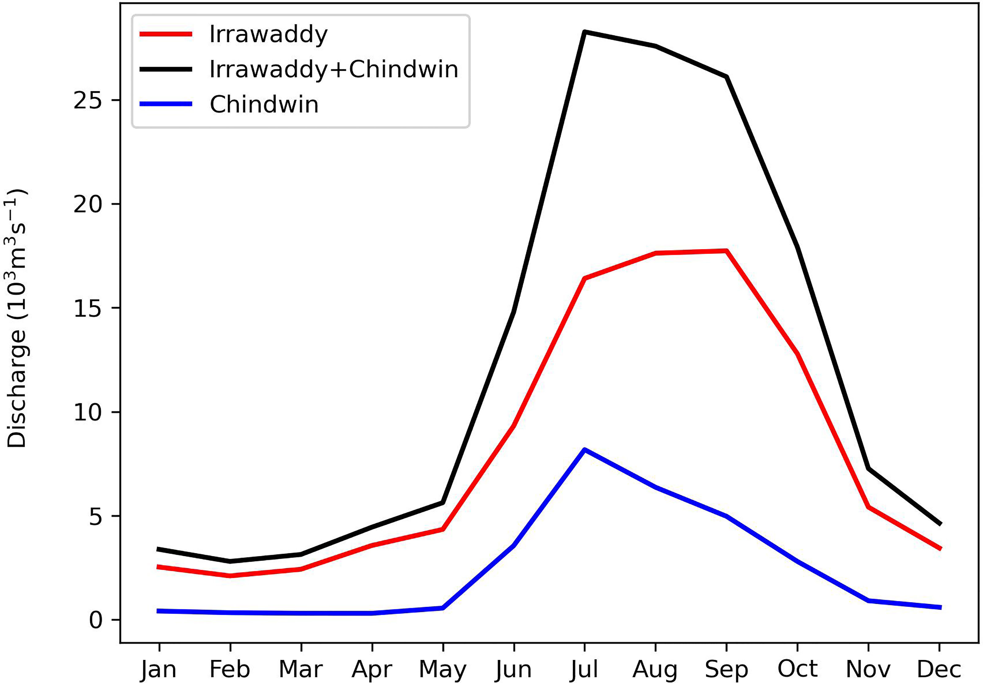
Figure 1 Seasonal cycle of freshwater discharge from Irrawaddy and Chindwin rivers in 10³ m³s^-1. Data for the discharge for these rivers is obtained from Dai and Trenberth Global River Flow and Continental Discharge Dataset (Dai and Trenberth, 2002; Dai et al., 2009).

The huge amount of freshwater gained by the Andaman Sea causes strong salinity stratification in the surface layer leading to the formation and maintenance of a barrier layer in the Andaman Sea (Sprintall and Tomczak, 1992). Varkey et al. (1997) presented the first comprehensive review of the physical oceanography of the Andaman Sea. They highlighted the large variations of density along the coast resulting from the large freshwater discharge from rivers in the summer monsoon. This region is also known for the occurrence of some of the largest internal solitons in the world. Shallow bottom topography near the Andaman Islands generates strong internal solitons that propagate in the Andaman Sea (Osborne and Burch, 1980; Alpers et al., 1997; Hyder et al., 2005). More recently, Jithin and Francis (2020), using observations and a numerical model, showed that the internal tides generated by the Andaman-Nicobar ridge caused enhanced vertical mixing in deeper ocean and kept the deeper Andaman Sea warmer than the surrounding Bay of Bengal. The Andaman Sea plays an important part in the dynamics of the rest of the Bay of Bengal. The circulation in the Bay of Bengal is influenced by the presence of coastal Kelvin waves excited by equatorial Kelvin waves, a phenomenon known as the remote forcing from the equatorial Indian Ocean (Potemra et al., 1991; Yu et al., 1991; McCreary et al., 1996; Shankar et al., 1996; Vinayachandran et al., 1996; Shankar et al., 2002). These coastal Kelvin waves travel along the eastern boundary of the Bay of Bengal, a significant part of which also forms the eastern boundary of the Andaman Sea. A modeling study by Chatterjee et al. (2017) shows that the coastal circulation in the Andaman Sea is primarily driven by the remote forcing from the equator. The Andaman Sea experiences strong southwesterly winds in the summer monsoon and northeasterly winds in the winter monsoon. Winds are weak during the transition period in spring and autumn. These winds, along with remote forcing, constitute an important forcing mechanism of the surface circulation in the Andaman Sea.

Despite its dynamical importance, the Andaman Sea has received a very little attention. In fact, the Andaman Sea has the lowest number of observations of salinity and temperature available in the tropical Indian Ocean, which itself is one of the least surveyed ocean regions in the world (Benshila et al., 2014; Liu et al., 2018). Many of the physical characteristics of the Andaman Sea and its circulation remain unexplored. Of particular importance is the surface salinity distribution during the summer monsoon, which is crucial for the formation of barrier layer in the Andaman Sea. A recent observational study of the seasonal variations of the upper ocean thermal structure and air-sea interactions over the Andaman Sea has emphasized the influence of surface salinity in the Andaman Sea on its mixed layer dynamics as well as air-sea interactions (Liu et al., 2018). Another observational study by Chandran et al. (2018) assessed the circulation and hydrography of the Andaman Sea during winter monsoon (November-December). Akhil et al. (2016b) investigated the dominant processes that control the interannual variability of the surface salinity in the Bay of Bengal and noted Irrawaddy discharge as the most important factor contributing to the variability of the surface salinity in the Andaman Sea during the summer monsoon. Ashin et al. (2019) studied the variability of the upper ocean in the Andaman Sea on seasonal and intraseasonal time-scales and highlighted the importance of the salinity in controlling the mixed-layer stratification. There have been many efforts of modeling surface salinity distribution in the Bay of Bengal and its response to forcing by sources of freshwater such as rivers and precipitation (Han and McCreary, 2001; Jensen, 2001; Howden and Murtugudde, 2001; Vinayachandran and Kurian, 2007; Benshila et al., 2014; Jana et al., 2015; Behara and Vinayachandran, 2016) but none of these studies focuses on the freshwater plume that arises due to discharge from IR river in the Andaman Sea. A modeling study by Benshila et al. (2014) mentions the wintertime evolution of the IR freshwater plume using a passive tracer. Previously, Chatterjee et al. (2017) have hinted at the need to investigate the effects of freshwater discharge from IR on the circulation in the Andaman Sea. Many of the important aspects of the IR plume in the Andaman Sea like horizontal extent and its seasonal variations, response to the seasonally varying winds, export pathways and dominant mechanisms of its dispersion remain unanswered. Freshwater in the Andaman Sea influences its mixed layer dynamics and air-sea interactions (Liu et al., 2018). Previous studies have shown that one of the important pathways of the transport of freshwater out of the Bay of Bengal is along the eastern coastline of the Andaman Sea (Pant et al., 2015; Jensen et al., 2016; Hormann et al., 2019). Modeling studies have highlighted the impact of freshwater gain through rivers on the variability of sea surface salinity (Seo et al., 2009; Vinayachandran and Nanjundiah, 2009) and SST (Vinayachandran et al., 2012) in the region. Being the largest source of riverine freshwater in the Andaman Sea, Irrawaddy discharge contributes significantly to the salinity and heat exchange between Bay of Bengal (including Andaman Sea) and the rest of the Indian Ocean. This makes the study of the behavior of Irrawaddy discharge in the Andaman Sea an important part of the regional oceanography.

There are several challenges in the study of the fate of discharge from the IR in the Andaman Sea during the summer monsoon. One of them is the significant freshwater input due to precipitation. The coastal regions of Andaman Sea receive a huge amount of precipitation during the summer monsoon. Similarly, the Andaman Sea receives a large amount of freshwater from other rivers and streams, the largest of them being the Sittang and Salween. Both of these rivers debouch their discharge into the Andaman Sea at the place located very close to the mouth of IR river. Along with IR discharge, freshwater from these rivers and precipitation creates a unified freshwater plume in the Andaman Sea during the summer monsoon and makes it extremely difficult to track the IR freshwater. A previous study by Pargaonkar and Vinayachandran (2021) isolated the Ganges-Brahmaputra River plume in the Bay of Bengal from precipitation and other rivers using a numerical ocean circulation model. In this study, we use a similar approach to investigate the fate of IR discharge in the Andaman Sea during the summer monsoon and the possible mechanisms behind it.

The set up of the numerical ocean circulation model used to study Irrawaddy River plume is described in Section 2. Section 3 contains analysis of the results from model experiments and is followed by discussion in Section 4 and summary in Section 5.

2 Model Description, Data and Validation

2.1 Model Setup

The Regional Ocean Modeling System (ROMS) was employed to conduct idealized numerical experiments for the study of the Irrawaddy River plume. The details of the computational engine and a host of parameterizations that ROMS provides can be found in Haidvogel et al. (2000) and Shchepetkin and McWilliams (2005). The setup employed in the present study is similar to the one used in the study of Ganges-Brahmaputra River plume by Pargaonkar and Vinayachandran (2021). A summary of the setup is described here. Model domain consists of the entire Indian Ocean stretching from 30°E to 120°E and 30°S to 30°N (inset region in the Figure 2). Model resolution is approximately 11km with 40 vertical levels. Vertical stretching parameters (V-transform, V-stretching, θ_s & θ_b) of the model are set in such a way that there are between 12 to 20 levels in the upper 20m of the ocean depending upon the sea surface height and the bathymetry. Vertical mixing of momentum and tracers is calculated using K-profile parametrization (KPP) model of Large et al. (1994). Horizontally, momenta and tracers are advected using a third order upwind scheme and mixed using harmonic mixing coefficients. The model has closed boundaries on the western and northern sides and open boundaries on the eastern and southern sides. At the open boundaries, salinity and temperature are nudged to the climatology obtained from Antonov et al. (2010). The free surface is forced with the daily climatology of the momentum and tracer fluxes obtained from ERA interim (Dee et al., 2011). At the free surface, model sea surface temperature is relaxed to the climatology from Antonov et al. (2010) using heat flux correction. The atmospheric parameters (winds, air density, specific humidity and air temperature) needed to compute the heat flux correction are obtained from ERA interim. In order to isolate the Irrawaddy plume, the freshwater flux from the atmosphere (evaporation minus precipitation or E minus P) is set to zero in all the experiments. The discharge from Irrawaddy River is applied at the 11 source points along the coastal wall at the location of the Irrawaddy River mouth. Discharge of Irrawaddy is a monthly climatology obtained from Dai and Trenberth (2002).

FIGURE 2

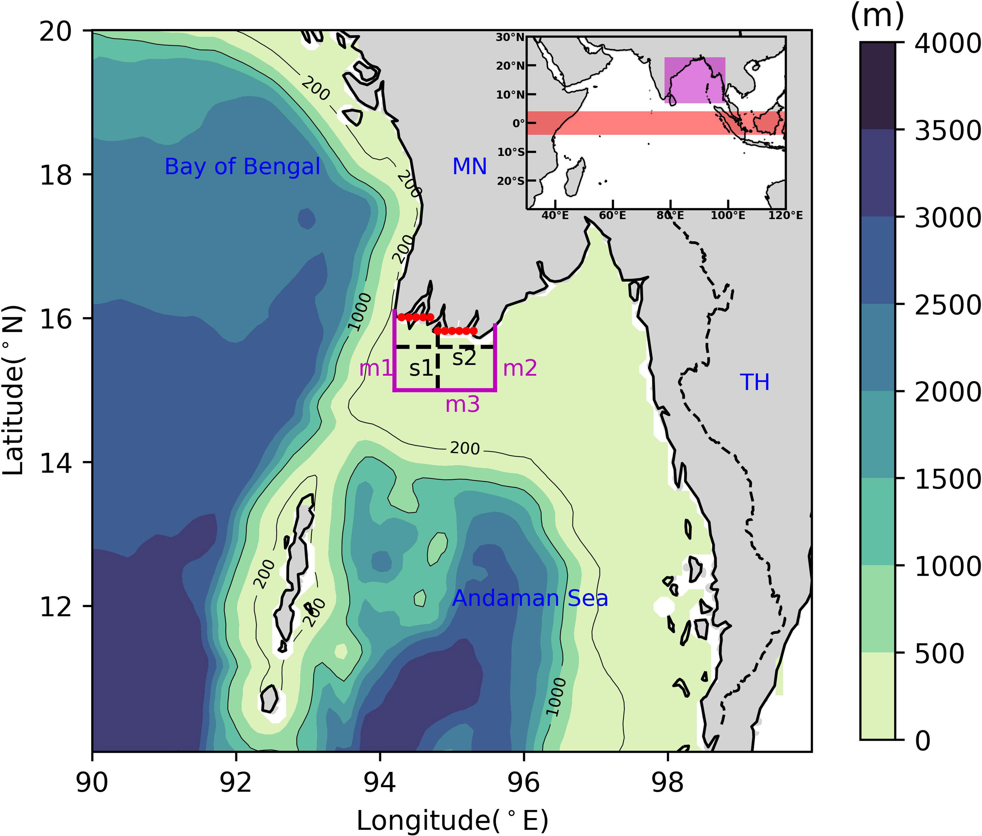
Figure 2 Study area for IR plume. Shading represents bathymetry in meters. Solid magenta lines represent sections m1, m2 and m3 along 94.2°E, 95.6°E and 15.0°N respectively. Thick dashed black lines represent sections s1 and s2 along 94.8°E and 15.6°N respectively. Thin black lines represent isobaths of 200m and 1000m. Red dots represent the positions of source points at which the river runoff is specified in the model. Inset shows model domain encompassing entire Indian Ocean (30°E– 120°E and 30°S–30°N). Area marked by red color in the inset is the equatorial region over which the wind forcing was applied in experiment IREqW and area marked by magenta is the area (encompassing the entire Bay of Bengal) over which the wind forcing was applied in experiment IRBoBW 1. Thin dashed black line represents international border between Myanmar and Thailand. Countries Myanmar and Thailand are shown by words ‘MN’ and ‘TH’ respectively.

Four different idealized experiments, each with a unique wind forcing scenario, were designed to study the effects of wind on the dynamics of IR River plume. These experiments vary primarily in the region over which wind forcing is applied. The choice of the region is based on previous studies investigating different wind forcing mechanisms of the Bay of Bengal (Potemra et al., 1991; Yu et al., 1991; McCreary et al., 1996; Shankar et al., 1996; Shankar et al., 2002). Details of the wind forcing for these experiments are presented in the Table 1. Each experiment starts with initial conditions obtained from the spin-up with no river forcing and a wind forcing unique to that experiment. The difference between experiment and spin-up is that when experiment starts, river discharge is included in the run. For example, for experiment IRFullW, initial conditions are obtained by spinning the model up for 10 years with winds all over the domain but without any river forcing. Experiment IRFullW then starts with the inclusion of IR river forcing and the same wind forcing as spin-up. Similarly, initial conditions for IRNoW are obtained from a 10 year spin-up of the model with no river and no wind forcing and then the experiment starts with the inclusion of IR river and no wind forcing. A similar description is applicable for other experiments. In order to better understand the dynamical influence of freshwater discharge from IR on the circulation and hydrography, another experiment (named SpinFullW) was setup. This experiment is the continuation of spin-up with wind forcing applied all over the model domain and without any river forcing for further 11 years.

TABLE 1

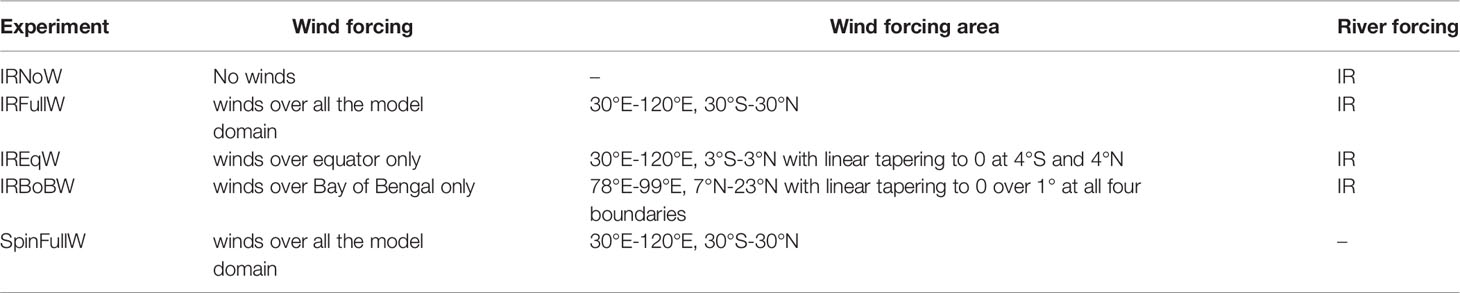
Table 1 Details of river and wind forcing for different experiments.

The study area for IR plume consists of a large portion of the Andaman Sea (90°E-100°E, 10°N-20°N). Three sections namely m1, m2, m3 near the river mouth are chosen across which freshwater transport calculations are performed. These sections are chosen such that they form a closed area around the river source points. In order to study vertical structure and dynamics of the plume at river mouth, two more sections were chosen— one in the meridional direction (section s1) and another in the zonal direction (section s2). Study area and the locations of these sections are shown in the Figure 2.

2.2 Data

In order to validate our model, as well as to confirm our findings regarding the horizontal orientation of the IR plume, we have compared model simulation with some of the freely available observational data. Details of this observational data are presented in this section.

For the validation of model simulation, we have used sea surface salinity (SSS) data from Soil Moisture Active Passive (SMAP) mission of the National Aeronautics and Space Administration (Fore et al., 2016). Monthly SMAP SSS data was obtained from the Asia-Pacific Data Research Center. This data has a spatial resolution of 0.25° and the data was obtained for the duration of January 2016 to December 2021. This SMAP data is compared to model simulated SSS obtained from experiment IRFullW. Since SMAP data is available for the duration of 6 years, we have used monthly SSS from the last 6 years of the simulation IRFullW. For the direct comparison of the SSS, 6 years worth of monthly data from both SMAP and model were converted to monthly climatology. In order to better understand where our model results stand in comparison to the observations, we have compared the standard deviation (SD) of the simulated and SMAP SSS. Before making these calculations (monthly climatology and SD), model SSS was interpolated to the 0.25° grid of the SMAP SSS data.

The experiment IRFullW performed for this study is an idealized experiment wherein the effects of precipitation and other major rivers in the region are neglected by omitting their forcing from the simulations. As such, this experiment cannot completely reproduce the salinity structure represented in the observations. Nonetheless, this experiment gives us an insight into the seasonal spread of IR water in the Andaman Sea especially the southeastward flow during the summer monsoon. The eastern shelf of Andaman Sea receives a large amount of freshwater through rainfall and through discharge from two major rivers: the Sittang and Salween. Since this freshwater forcing is absent from our simulations, it is safe to assume that the salinity structure over the eastern shelf of Andaman Sea cannot be fully captured by IRFullW experiment. However, it is possible that the southeastward spread and the westward extent of IR plume during the summer monsoon could be well captured by IRFullW. To confirm this, we use monthly climatology of Chlorophyll-a concentration from Moderate Resolution Imaging Spectroradiometer (MODIS) launched on board Aqua satellite in 2002 by NASA. Surface distribution of chlorophyll-a concentration has previously been used successfully to understand the dynamics of the Mississippi River plume (Walker et al., 2005; Schiller et al., 2011).

To further confirm our findings, we have also used surface currents from an ocean reanalysis data (GLOBAL-REANALYSIS-PHY-001-030) provided by Copernicus Marine Services. This data product is a global ocean eddy-resolving reanalysis obtained using the Nucleus for European Modelling of the Ocean (NEMO) model that incorporates assimilation of satellite derived sea level anomaly, sea surface temperature, sea ice concentration, and in situ vertical temperature and salinity profiles (Ferry et al., 2012; Madec and Team, 2019). This reanalysis data is available from January 1993 to December 2018 at both daily and monthly frequencies. To compare with IRFullW climatology of surface currents, we obtained the monthly reanalysis data from January 2001 to December 2010 and made a climatology of surface currents. Many of the previous studies have successfully used NEMO simulations to investigate various features of the circulation in the Bay of Bengal. Previously, Webber et al. (2018) have successfully used the NEMO model simulations for the study of the southwest monsoon currents in the Bay of Bengal. Sanchez-Franks et al. (2019) have also used the NEMO model simulations to trace the origins and to study the variability of the high saline core of the southwest monsoon currents. Using salinity, temperature, currents, and sea level anomalies, Greaser et al. (2020) studied interactions between mesoscale eddies in the Bay of Bengal and the synoptic scale disturbances during the summer monsoon season of 2019. Momin et al. (2021) assessed NEMO simulated surface currents with the help of radar generated surface currents data along the eastern coast of India.

2.3 Model Validation

In this section, we present the validation of Sea Surface Salinity (SSS) simulated by our model. For the purpose of validation, model simulated SSS from experiment IRFullW is used.

As described previously, experiment IRFullW is an idealized experiment in which the effects of freshwater due to precipitation and other rivers, except Irrawaddy, are ignored. Because of this idealized setting, this experiment cannot fully reproduce the patterns of SSS observed in the in-situ or satellite data. Despite this, the experiment IRFullW does help us better understand the movement of the freshwater due to Irrawaddy River discharge with respect to the movement of the total freshwater in the Andaman Sea during the summer monsoon and the mechanisms behind this movement. Panels A and B in Figure 3 represent maps of the SSS climatology from SMAP and experiment IRfullW averaged over the months of summer monsoon season (June-September). During the summer monsoon, the model produces lower SSS values compared to SMAP everywhere in the Andaman Sea except near the Irrawaddy mouth. We attribute this large difference in the SSS to the absence of precipitation as well as other rivers in the vicinity of the Irrawaddy mouth in our simulation. Previous studies have established that during the summer monsoon, a large freshwater pool forms near the mouth of Ganges River and expands southward along the coast north of the Irrawaddy River mouth (Akhil et al., 2014; Jana et al., 2015; Behara and Vinayachandran, 2016; Pargaonkar and Vinayachandran, 2021). This region also receives a large amount of freshwater due to precipitation (Qi and Wang, 2015). This leads to lower SSS values in the northern part (north of 16°N) of the region as shown in the Figure 3A. Since IRFullW starts after the spin-up without any river forcing, it has higher SSS values in the same region (Figure 3B). Similarly, the eastern coast of the Andaman Sea receives huge freshwater influx due to precipitation as well as the discharge from the Sittang and Salween Rivers (Qi and Wang, 2015; Baronas et al., 2020). This leads to lower SSS values along the coast especially to the east of the Irrawaddy River mouth where both the Sittang and Salween debouch into the Andaman Sea (Figure 3B). Overall, the difference between model SSS and SMAP SSS are of the order of 2.5 psu over the open ocean and the northern coast, whereas those east of the Irrawaddy River mouth are of the order of 4 psu. Despite these differences, the model simulation does reproduce the northwest-southeast orientation of the freshwater plume in the Andaman Sea reasonably well. It also tells us that the major portion of the Irrawaddy discharge flows towards the southeast during the summer monsoon. Panels C and D in Figure 3 represent the standard deviation (SD) of SMAP and model SSS. SMAP SSS shows the SD of more than 2.5 psu all along the eastern coast of the Andaman Sea (Figure 3C). In comparison, the model SSS shows SD of lower than 1 psu all over the domain except near the Irrawaddy River mouth (Figure 3D). These large differences between the variability of the SSS from model and SMAP can again be attributed to the way our experiment was designed as discussed above. This comparison also shows that the precipitation plays an important role in modulating the SSS of coastal Andaman Sea. In fact, as previously established by Behara and Vinayachandran (2016), freshwater due to precipitation over the Bay of Bengal is predominantly exported out of the bay along the eastern coast. Though the values of SSS in SMAP and model do not exactly match, the salinity contours at the easternmost edge of the freshwater jet in model align reasonably well with the salinity contours from SMAP (Figures 3A, B). Similarly, the western part of the pattern of SD of SMAP SSS aligns well with that of model SSS (Figures 3C, D). This indicates the existence of a freshwater jet in the Andaman Sea, even though the eastern part of the jet is buried in the lower salinity caused by freshwater input from the Sittang and Salween Rivers, as well as precipitation. Further confirmation of the existence of freshwater jet is done using surface currents from reanalysis in Section 3.2.

FIGURE 3

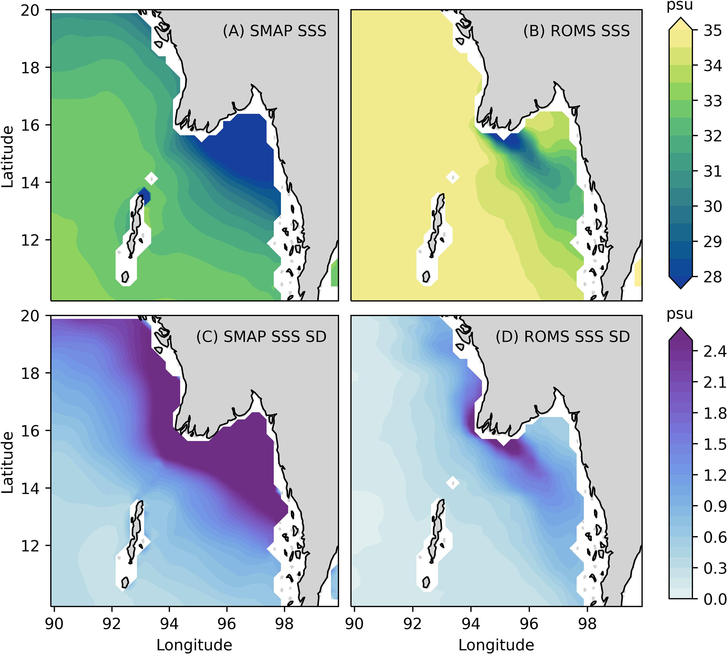
Figure 3 Comparison of SSS climatology from (A) SMAP and (B) model experiment IRfullW for summer monsoon (averaged over June-September). Model climatology is obtained from the last 6 years of experiment IRFullW and then interpolated to the 0.25° resolution grid of the SMAP SSS. SMAP SSS climatology is obtained from the monthly SSS data between January 2016 and December 2021. (C) standard deviation (SD) of SSS from SMAP monthly data obtained for the duration of January 2016 to December 2021. (D) Standard deviation of SSS from the monthly data of the last 6 years of experiment IRFullW.

3 Results

3.1 Horizontal Structure

To characterize the horizontal structure of the IR plume during the summer monsoon, we used surface salinity and surface currents from the first year of experiment IRFullW (i.e., the first year after the introduction of IR river forcing). The boundary of the plume is demarcated using 32 psu isohaline.

During the summer monsoon (June-August), winds over the study area are strong and start weakening from September. Summer monsoon is also the season when discharge from the IR increases rapidly. In June, with increased discharge from the IR and strong south-westerly winds, the freshwater plume starts to expand rapidly towards south-east (Figure 4A). This expansion occurs in the form of a jet like structure of low salinity water and is distinguishable from the surrounding regions by the presence of high-speed currents (0.5 ms^-1) that comprise the core of this jet. Currents at the southern flank of the jet, although weak, turn towards south-east and arrest the westward expansion of the freshwater plume. In the month of July, IR discharge reaches its peak, winds strengthen slightly compared to the previous month, and the IR plume flows as a jet of low salinity water with strong south-eastward currents at its core. IR plume flows further south-east to reach the eastern boundary of the Andaman Sea and widens at its southern end with its northern flank reaching the eastern coast at 14°N and southern flank at 12°N (Figure 4B). The strength of the current reduces as it approaches the coast. In August, the IR plume expands further south along the eastern boundary of the Andaman Sea (Figure 4C). The jet-like flow of the plume still persists but near the eastern coast, it widens and forms two distinct flanks with a weak circulation in between. Currents in the northern flank flow eastward to reach the coast and then flow southward. Currents in the southern flank continue to flow south-eastward. Low salinity water (≤ 33 psu) reaches as far south as 11°N. Throughout August, a large amount of freshwater accumulates over the shelf adjacent to the eastern coast. In September, southwesterly winds over the Andaman Sea weaken and the discharge from the IR is also on the decline (Figure 1). The IR plume still flows as jet of low salinity water impinging on the coast at the eastern boundary of the Andaman Sea at 13°N (Figure 4D). A very small amount of freshwater from the northern boundary of the plume leaks northward along the coast while most of it continues to flow southward and reaches as far south as 10°N. Eastward currents at 13°N flow into the plume and turn southward thus making the southern flank of the IR plume.

FIGURE 4

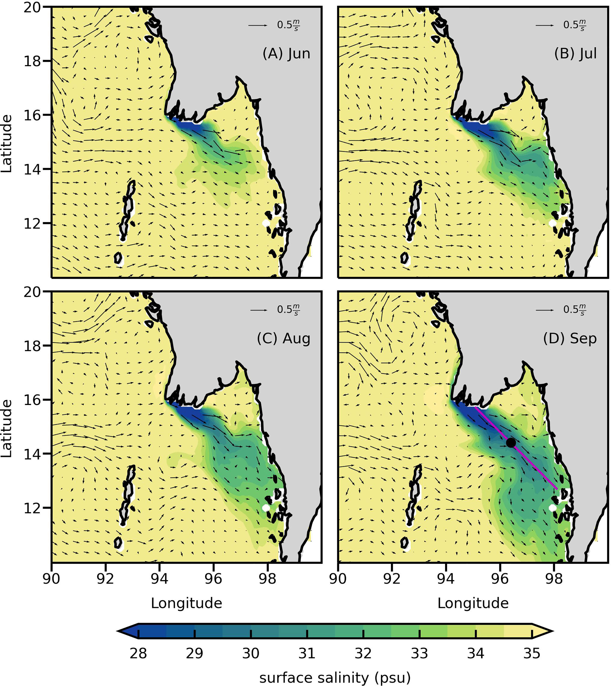
Figure 4 Maps of monthly averaged sea surface salinity (psu) and surface currents (ms^-1) from the first year of experiment IRFullW. Solid magenta line in panel (D) represents an axis of the IR jet along which the time evolution of the jet has been analyzed. The black dot on this axis shows the location where the annual cycle of the momentum terms has been presented.

3.2 Observational Evidence for the IR Jet in the Summer Monsoon

Figure 5 shows the spatial distribution of sea surface salinity climatology from IRFullW overlaid by contours of Chlorophyll-a climatology from MODIS during the summer monsoon. Two contours of Chlorophyll-a are plotted. One of the contours represents a value of 0.2 mgm^-3 and is the indicator of the spread of freshwater over open ocean. The other contour with value 0f 1.0 mgm^-3 is plotted to demarcate the region of higher Chlorophyll-a concentration and lower surface salinity arising due to the omitted freshwater forcing as discussed above. For all four months of the summer monsoon, 0.2 mgm^-3 contour of Chlorophyll-a aligns with the western and southern edges of the IR freshwater plume. The closest match between 0.2 mgm^-3 contour and the western extent of the IR plume over open ocean can be seen in the month of September (Figure 5D). The orientation of 0.2 mgm^-3 contour also suggests the presence of freshwater with northwest-southeast orientation during the summer monsoon. Moreover, the widening of IR plume from June to September is also consistent with the increased spacing between the two chlorophyll-a contours during the same period. A good agreement between the shape of IR freshwater jet and the region of freshwater demarcated by the chlorophyll-a contours is an indication of the existence of IR freshwater jet in the Andaman Sea during summer monsoon.

FIGURE 5

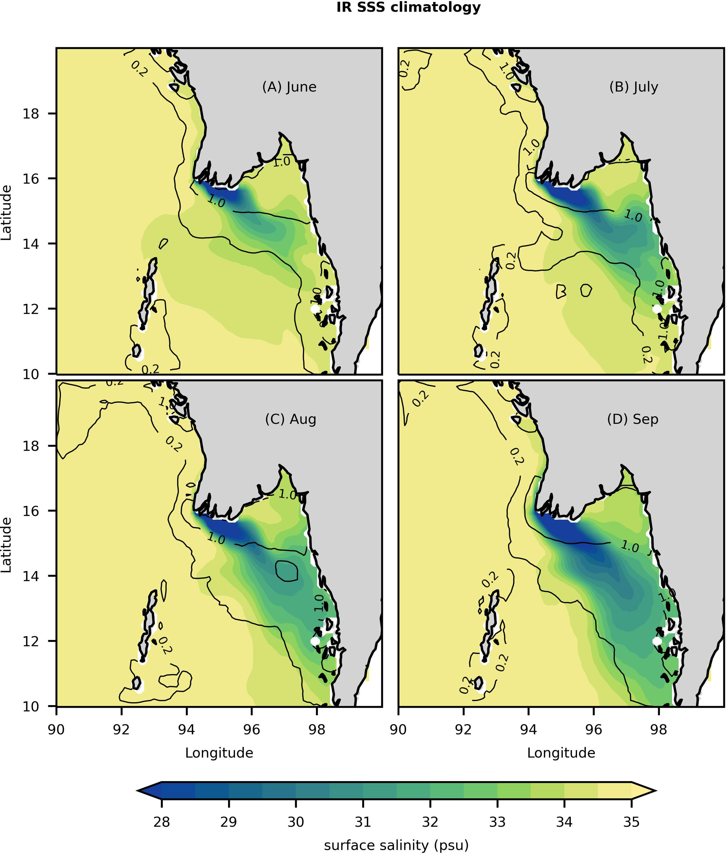
Figure 5 Maps of sea surface salinity climatology (shading) obtained from experiment IRFullW and Chlorophyll-a climatology (black contours) obtained from MODIS for the months of summer monsoon. Units of Chlorophyll-a concentration are mgm^-3. MODIS data was interpolated to ROMS grid and smoothed using a 5 point boxcar smoother in both East-West and North-South directions before plotting.

NEMO data also shows indications of the presence of IR jet in the Andaman Sea during the summer monsoon. Figure 6 shows the distribution of surface currents from IRFullW and the reanalysis data for the month of September. Surface current distribution from IRFullW agrees well with that from the reanalysis data, especially over the Andaman Sea region. The reanalysis data also shows an existence of a jet-like structure emanating from the IR river mouth and flowing towards southeast (Figure 6B). Although the jet in reanalysis data is weaker compared to the jet in IRFullW, it’s orientation closely matches that of IR jet from our simulation. We would like to note that the reanalysis data contains freshwater from other major rivers from the area as well as from the precipitation. Even then, IRFullW captures other features of surface circulation in the Andaman Sea quite well. Clearly, this comparison of surface currents from IRFullW and a global simulation with data assimilation from NEMO is a good indicator of the presence of IR freshwater jet during summer monsoon. At this point, we would like to note that high resolution observations of surface currents in the Andaman Sea are required to further confirm the existence of IR freshwater jet. This is especially true given the complex physics underlying the circulation of the Andaman Sea because of the presence of shallow bathymetry over most of the region, seasonally varying winds, and it’s proximity to the equator.

FIGURE 6

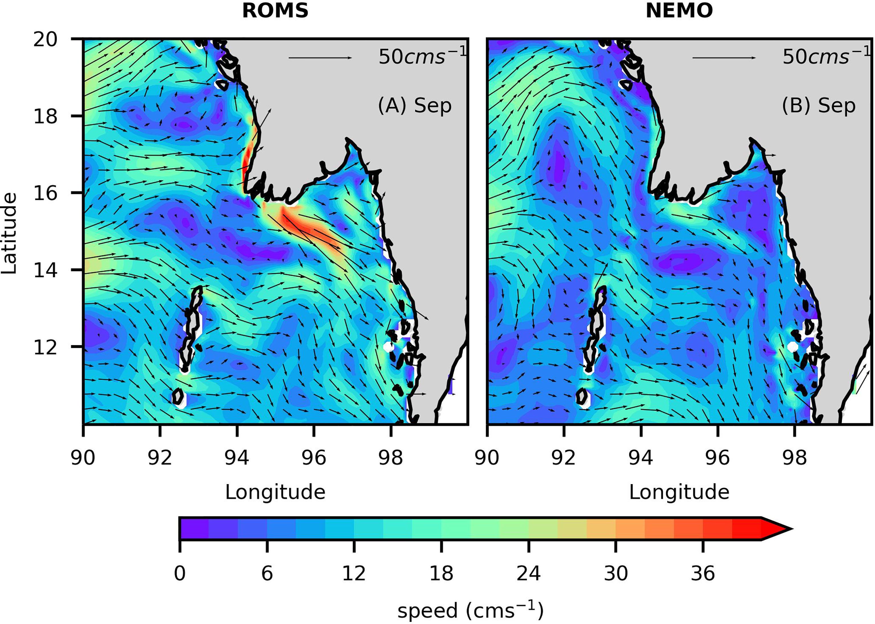
Figure 6 Comparison of the spatial distribution of climatology of surface currents from IRFullW (left panel) and GLOBAL-REANALYSIS-PHY-001-030 (right panel) for the month of September.

3.3 Mechanisms of the Formation of the IR Jet

In order to understand the mechanisms behind the formation of the IR freshwater jet during the summer monsoon, we have analyzed the evolution of the jet using surface salinity, currents, and wind stress along an axis of the IR jet. Figure 7 shows Hovmöller diagrams of surface salinity, surface current speed, and wind stress magnitude with x-axis being the distance along the axis of IR jet. Throughout the summer monsoon, wind stress magnitude is mostly constant along the first half of axis with a slight reduction over the remaining half. Surface salinity evolution clearly shows the spread of freshwater from the IR source points to the shelf throughout summer monsoon. Further, it also shows the IR plume receding along the axis during winter monsoon. A comparison of evolution of surface salinity with that of the surface current speed shows that the higher speed exists where the surface salinity is lower. Since the magnitude of wind stress along the axis is almost constant (constant momentum input), higher speeds in the region of freshwater indicate trapping of this momentum by a strongly stratified IR plume. This further confirms that the presence of freshwater from IR focuses momentum input from winds to drive the IR plume towards southeast during the summer monsoon. Recently, Chaudhuri et al. (2021) have shown that the salinity stratified layer prevents the shear- induced mixing in the upper fresh layer and traps the momentum input by winds. They also show the presence of an extremely shallow Ekman layer in the region of freshwater and that the velocity at the base of such a shallow layer is directed at approximately 80° to wind vectors. This indicates that the southwesterly winds push freshwater towards southeast as the vertically integrated transport in the shallow Ekman layer is dominantly towards southeast.

FIGURE 7

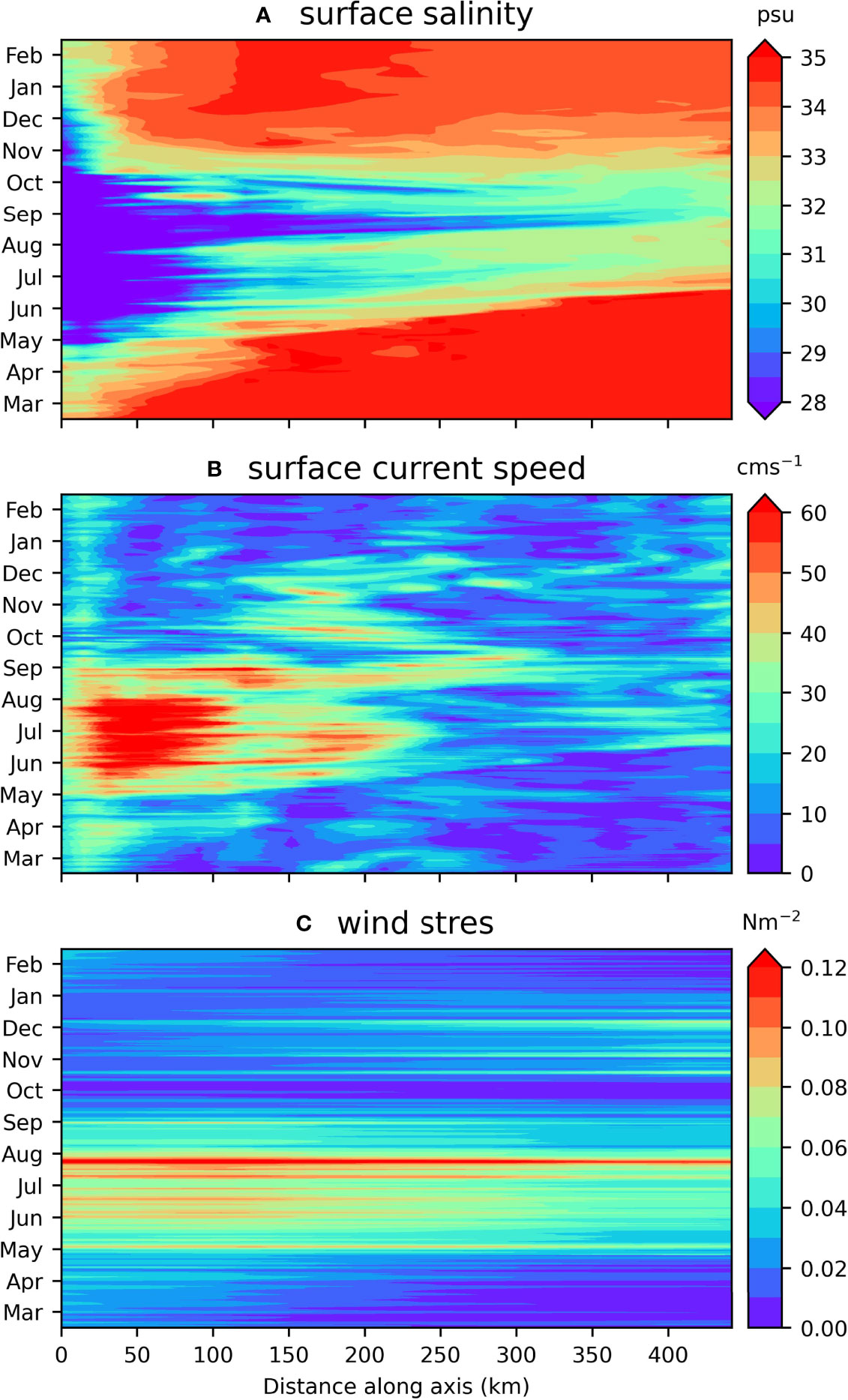
Figure 7 Time evolution of surface salinity (top panel), surface current speed (middle panel) and wind stress magnitude (bottom panel) along an axis of IR plume shown in Figure 4D. Salinity and current data is taken from the first year of experiment IRFullW.

To confirm that the wind forcing drives the IR jet during summer monsoon, we have analyzed the distribution of the dominant terms from both the zonal and meridional momentum equations at the location very close to the river mouth (sections s1 and s2 in Figure 2). Further, we have also analyzed the annual cycle of the dominant terms from both the momentum equations at a point completely inside the IR freshwater jet.

3.3.1 Momentum Balance Near the River Mouth

An analysis of the distribution of terms from the momentum equations across sections s1 and s2 (Figure 2) is presented here. Many of the previous numerical studies have used momentum balances in the vicinity of the source points to explain the dynamics of the plume (Hetland, 2005; Choi and Wilkin, 2007; Denamiel et al., 2013; Androulidakis et al., 2015; Pargaonkar and Vinayachandran, 2021). Horizontal momentum equations that ROMS solves are given below (Shchepetkin and McWilliams, 2005). These equations are presented in the Cartesian coordinate system and after the application of Boussinesq approximation.

$\begin{array}{ll}\begin{array}{l}\underset{\text{acceleration}}{\underbrace{\frac{\partial u}{\partial t}}}+\underset{\text{horizontal}\hspace{0.17em}\text{advection}}{\underbrace{u\frac{\partial u}{\partial x}+v\frac{\partial u}{\partial y}}}+\underset{\text{vertical}\hspace{0.17em}\text{advection}}{\underbrace{w\frac{\partial u}{\partial z}}}-\underset{\text{Coriolis}}{\underbrace{fv}}\\ =\underset{\text{pressure}\hspace{0.17em}\text{gradient}}{\underbrace{-\frac{1}{{\rho }_0}\frac{\partial p}{\partial x}}}+\underset{\text{horizontal}\hspace{0.17em}\text{diffusion}}{\underbrace{\frac{\partial }{\partial x}\left(K_H\frac{\partial u}{\partial x}\right)+\frac{\partial }{\partial y}\left(K_H\frac{\partial u}{\partial y}\right)}}+\underset{\text{wind}\hspace{0.17em}\text{friction}}{\underbrace{\frac{\partial }{\partial z}\left(K_z\frac{\partial u}{\partial z}\right)}}\end{array}& (1)\end{array}$

$\begin{array}{ll}\begin{array}{l}\underset{\text{acceleration}}{\underbrace{\frac{\partial v}{\partial t}}}+\underset{\text{horizontal}\hspace{0.17em}\text{advection}}{\underbrace{u\frac{\partial v}{\partial x}+v\frac{\partial v}{\partial y}}}+\underset{\text{vertical}\hspace{0.17em}\text{advection}}{\underbrace{w\frac{\partial v}{\partial z}}}+\underset{\text{Coriolis}}{\underbrace{fu}}\\ =\underset{\text{pressure}\hspace{0.17em}\text{gradient}}{\underbrace{-\frac{1}{{\rho }_0}\frac{\partial p}{\partial y}}}+\underset{\text{horizontal}\hspace{0.17em}\text{diffusion}}{\underbrace{\frac{\partial }{\partial x}\left(K_H\frac{\partial v}{\partial x}\right)+\frac{\partial }{\partial y}\left(K_H\frac{\partial v}{\partial y}\right)}}+\underset{\text{wind}\hspace{0.17em}\text{friction}}{\underbrace{\frac{\partial }{\partial z}\left(K_z\frac{\partial v}{\partial z}\right)}}\end{array}& (2)\end{array}$

A careful examination of the terms of the momentum equations revealed that the dominant terms in u and v momentum equations are Coriolis (fv, -fu), pressure gradient $\left(-\frac{1}{{\rho }_0}\frac{\partial p}{\partial x},-\frac{1}{{\rho }_0}\frac{\partial p}{\partial y}\right)$, horizontal advection $\left(-u\frac{\partial u}{\partial x}-v\frac{\partial u}{\partial y},-u\frac{\partial v}{\partial x}-v\frac{\partial v}{\partial y}\right)$, and wind friction $\left(\frac{\partial }{\partial z}\left(K_z\frac{\partial u}{\partial z}\right),\frac{\partial }{\partial z}\left(K_z\frac{\partial v}{\partial z}\right)\right)$. Monthly averages of other terms like acceleration and vertical advection were found to be an order of magnitude smaller than these four terms (10^-6 – 10^-9 ms^-2 compared to 10^-5 ms^-2 for the four terms mentioned above) and hence, are not presented here.

Panels A–D in Figure 8 show meridional momentum balance in experiment IRFullW at s1 for the month of August. The Coriolis term is predominantly negative with higher values near the river mouth and the upper 5m of the section (Figure 8A). Small positive values exist in a narrow band near the coast and below the depth of 5m. The pressure gradient term is negligible at the surface (Figure 8B. Both pressure gradient and Coriolis terms are comparable below the depth of 5m across the section and both terms balance each other at this location. Nonlinear advection is also negligible throughout the section (Figure 8C). Wind friction term is predominantly positive at the surface throughout the section (Figure 8D). In fact, the distribution of wind friction is similar to Coriolis term in the upper 4m of the section. Both Coriolis and wind friction terms have similar magnitude at the surface. This positive wind friction translates to positive (eastward) currents at the surface through Ekman balance. Considering the value of Coriolis term at the surface near the river mouth (-1.2×10^-5 ms^-2) and Coriolis frequency of 0.396×10^-4 s^-1, the estimate of surface current turns out be 30cm/s. To summarize, Ekman dynamics determines the balance of cross-shore momentum in the IR plume at the location river mouth.

FIGURE 8

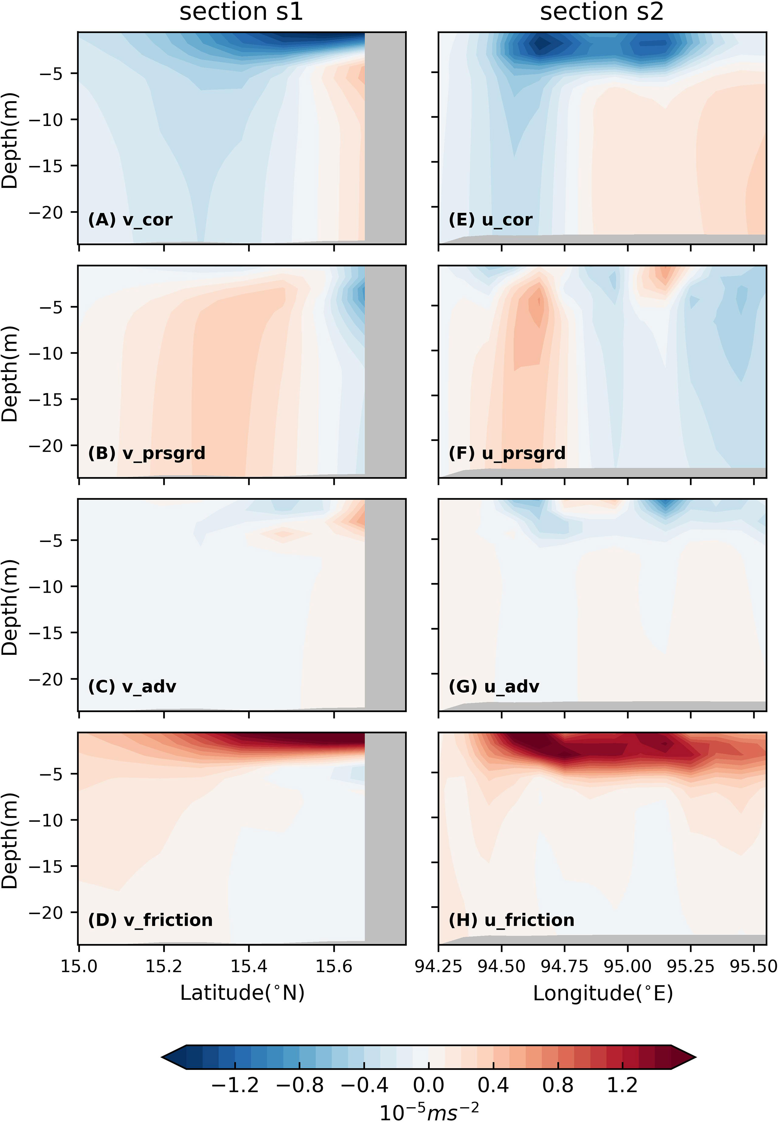
Figure 8 Left Column: Distribution of meridional (v) momentum terms from experiment IRFullW for the month of August. Panels (A–D) show distribution of Coriolis, pressure gradient, horizontal advection and wind friction at the section s1. Right Column: Distribution of zonal (u) momentum terms from experiment IRFullW for the month of August. Panels (E–H) show distribution of Coriolis, pressure gradient, horizontal advection and wind friction at the section s2.

Panels –E–H in Figure 8 show the zonal momentum balance in experiment IRFullW at s2 for the month of August. Coriolis term shows high negative values in the near surface layer (up to 4m deep) between 94.6°E and 95.3°E where river source points are located (Figure 8E). Pressure gradient term shows patches of low negative and positive values near the surface (Figure 8F). Nonlinear advection also appears in the form of patches of low negative and positive values but is confined to a much thinner layer as compared to pressure gradient (Figure 8G). The dominant term appears to be wind friction and is distributed in a pattern similar to that of the Coriolis term (Figure 8H). Negative Coriolis term and positive wind friction term appear to be in balance though wind friction term has slightly higher magnitude than Coriolis term. High positive value of wind friction in u-momentum drives southward currents in the near surface layer. In summary, Ekman balance dominates the alongshore momentum in the IR plume near river mouth.

To summarize, winds, through Ekman dynamics, drive the plume during summer monsoon season. Distribution of wind friction term remains confined to the region with high salinity stratification caused by IR discharge.

3.3.2 Momentum Balance in the IR Jet

In order to further understand the balance of momentum inside the IR plume, an annual cycle of the four important momentum terms at a point inside the IR jet is presented. The location of the point is chosen such that the point lies approximately in the middle of the jet in August.

Figure 9 shows annual cycle of the four dominant terms of momentum equations from experiment IRFullW, averaged over the first five levels from the surface, at a point (black dot in Figure 4D, located at 96.4°E,14.4°N) in the IR jet. The top panel from Figure 9 shows terms of u-momentum equation. From March through May, the wind friction term remains positive with very little change in magnitude whereas the Coriolis term changes the sign twice. Pressure gradient and Coriolis have similar magnitudes with the wind friction term contributing equally. After the arrival of summer monsoon in June and an increase in IR discharge, the wind friction term becomes more positive and the Coriolis term more negative with both terms having equal magnitude. The positive wind friction and negative Coriolis term in u-momentum equation give rise to a southward velocity in IR jet. Throughout the summer monsoon, the wind friction term is balanced by the Coriolis term. Pressure gradient and horizontal advection terms remain small. Thus, throughout the summer monsoon, IR flows under the influence of winds and Coriolis force. After the summer monsoon, the geostrophic balance is restored at the location and wind friction is relevant only in November when it balances a positive Coriolis term and a positive pressure gradient term.

FIGURE 9

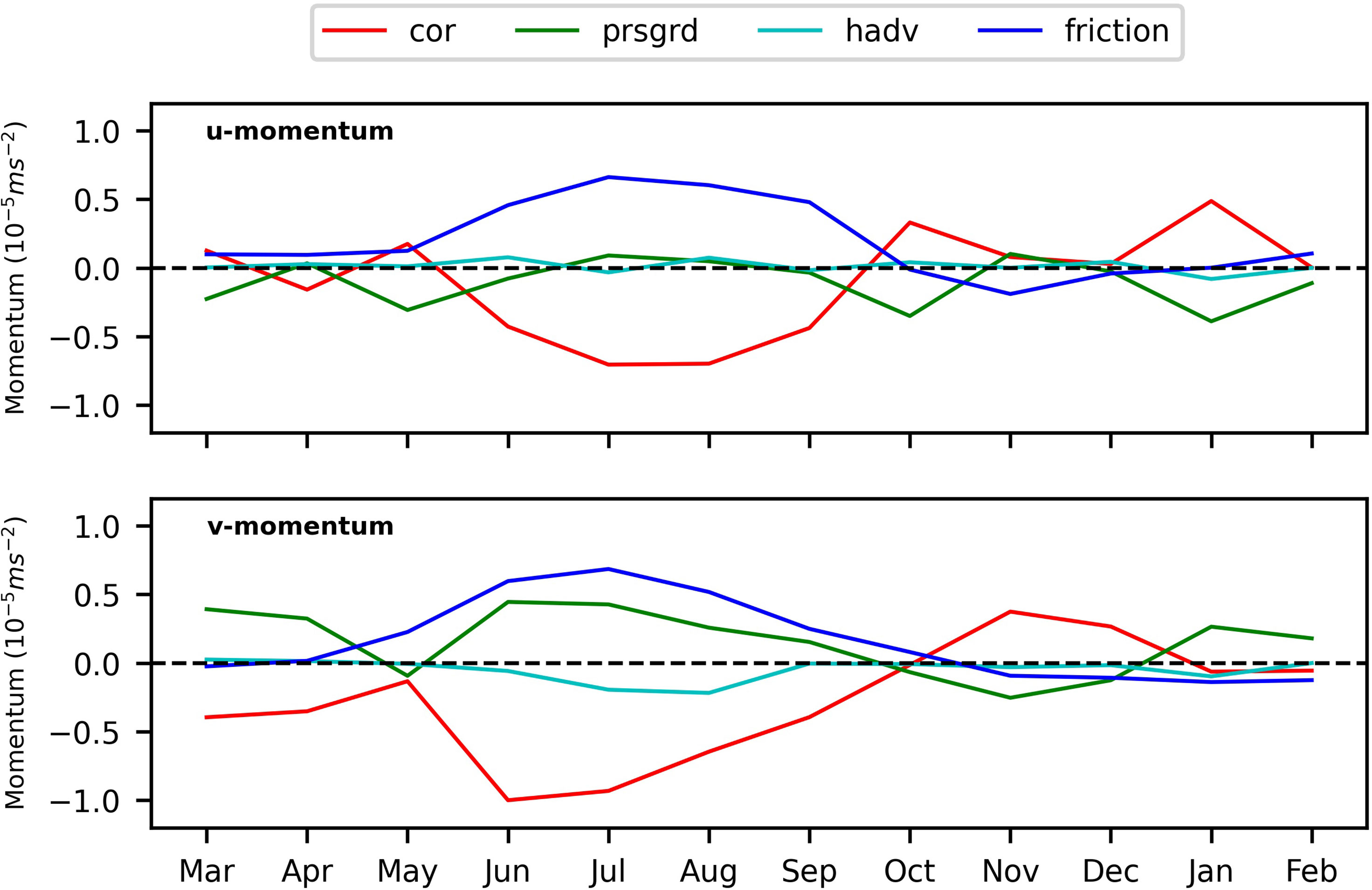
Figure 9 Annual cycle of the four momentum terms namely Coriolis(red), pressure gradient(green), horizontal advection(cyan) and wind friction(blue) at a point (black dot in Figure 4D) in IR jet. Upper panel shows the annual cycle of momentum terms from the zonal momentum (u-momentum equation) and the lower panel shows the annual cycle of the meridional momentum (v-momentum equation). All terms are averaged over the first five levels from the surface.

The bottom panel from Figure 9 shows terms of v-momentum equation. From March through April, the meridional momentum balance is completely geostrophic. With the establishment of south-westerly winds over the location in May, wind friction term increases in magnitude. Throughout the summer monsoon, wind friction remains positive and Coriolis term remains negative with the later having larger magnitude. The pressure gradient term also increase throughout the summer monsoon and remains positive with smaller magnitude than the wind friction term. A negative Coriolis term and a positive wind friction term in v-momentum equation contribute to a positive or eastward zonal velocity in IR jet. Throughout the summer monsoon, a large negative Coriolis term is balanced by a positive wind friction term with an added assistance of pressure gradient term. After the summer monsoon, the meridional momentum balance is mostly geostrophic.

A similar analysis of the momentum terms at several locations along the IR jet axis (as shown in Figure 4D) shows a similar annual behavior as discussed above. Inside IR jet, wind friction dominates over the pressure gradient in balancing a large Coriolis term during the summer monsoon. The result of this balance is a southeastward flow of the IR water through the large contribution of wind friction and Coriolis terms towards southward and eastward flow. Freshwater from IR flows southeastward throughout summer monsoon under the influence of winds through Ekman dynamics and the flow of the plume in the rest of the year is under the influence of geostrophy. In summary, the freshwater discharge from the IR traps the momentum input from winds over the region of high stratification. This results in faster currents in the region occupied by the freshwater and gives it an appearance of a freshwater jet. The orientation of winds (southwesterly) causes the IR freshwater jet to be oriented towards southeast.

3.4 The Effects of Wind

Previous investigations have established the importance of the local, as well as remote, forcing from the equator in determining circulation patterns over the Bay of Bengal and the Andaman Sea (Potemra et al., 1991; Yu et al., 1991; McCreary et al., 1996; Shankar et al., 1996; Vinayachandran et al., 1996; Shankar et al., 2002; Cheng et al., 2013; Chatterjee et al., 2017). In order to study the response of the IR plume to the important wind forcing mechanisms of the region and to understand whether they contribute to the formation of IR jet in the summer monsoon, experiments IRNoW, IREqW and IRBoBW were performed with no winds, winds only over equator, and winds only over Bay of Bengal, respectively. The effects of wind on plume characterization are presented in the form of surface salinity and currents for the month of August.

In order to understand the behavior of the IR plume in the absence of winds, an experiment (IRNoW) with no wind forcing was set up. The initial conditions for this experiment were obtained by spinning the model up for 10 years and 2 months without IR discharge and without any wind forcing. Model integration for the experiment starts with these initial conditions and with the introduction of IR discharge. To complete the experiment, the model was integrated for 11 more years. Similarly, two more experiments with only equatorial wind forcing and only BoB wind forcing, respectively, were conducted. An important difference between the experiments IRfullw and IRBoBW is the absence of equatorial forcing in the latter. Equatorial forcing is an important part of the forcing mechanisms of the circulation in the Andaman Sea and it manifests itself predominantly in the month of May. The month of May marks the intrusion of a northward propagating signal from the equator in the Andaman Sea along its eastern boundary (McCreary et al., 1996; Chatterjee et al., 2017). This signal manifests itself in the form of a high sea level anomaly along the east coast of the Andaman Sea and a strong northward current. Figure 10 shows the sea surface height anomaly for the month of May from the first year of all four experiments. The equatorial signal is strongest in the experiment IREqW and is absent from the experiments IRBoBW and IRNoW (Figures 10B–D). In experiment IRFullW, equatorial signal is present but is weaker compared to that in the experiment IREqW (Figures 10A, B). Looking at the structure of the anomalies in experiment IRBoBW, we can attribute the weaker equatorial forcing in IRFullW to the presence of wind forcing over the domain as it generates negative anomalies and weakens the strong positive intrusion from equator.

FIGURE 10

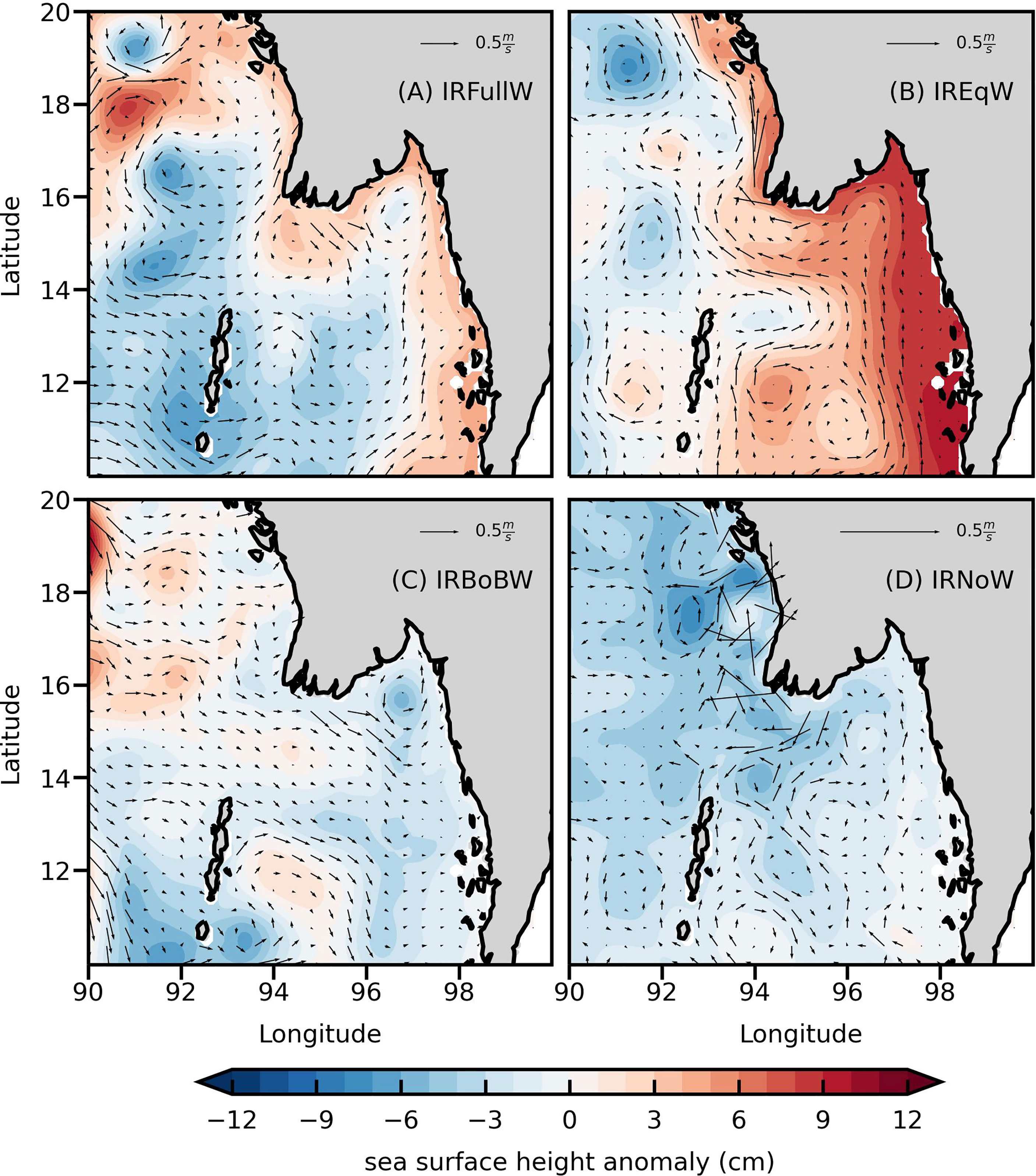
Figure 10 Maps of monthly averaged sea surface height anomaly and surface currents(ms^-1) for the month of May from the first year of experiments.

Figure 11 shows surface salinity and currents from these three wind sensitivity experiments for the first year of the simulation. In the absence of winds, the IR outflow forms a large pool of freshwater around the river mouth and a downstream current in the month of August (Figure 11A). Freshwater, after exiting from the mouth, circulates inside the pool of freshwater and then flows downstream. Circulation in the pool of freshwater around river mouth is anticyclonic. Previous studies have established the presence of an anticyclonic bulge and a downstream current coastal current as a classic response of a river plume in the absence of winds (Oey and Mellor, 1993; Kourafalou et al., 1996; Fong, 1998; Garvine, 2001; Yankovsky et al., 2001; Fong and Geyer, 2002; Garcia Berdeal et al., 2002; Denamiel et al., 2013). The downstream flow along the coast of Myanmar reaches the northern boundary of the study area at 20°N. As the discharge continues to increase throughout the summer monsoon, the anticyclonic bulge of freshwater around river mouth expands and the downstream current becomes wider (not shown here). Some of the freshwater from the bulge leaks from its westward end and flows south to reach the northern tip of the Andaman Islands (Figure 11A). At this stage, a major portion of the freshwater from the river discharge circulates in the anticyclonic bulge and the rest flows as a downstream coastal current. In the presence of only equatorial winds, discharge from rivers forms an anticyclonic bulge and a downstream coastal current (Figure 11B). The coastal current extends from the anticylonic bulge to the northern boundary of the study area at 20°N. Some of the freshwater from the anticyclonic bulge leaks southward. A cyclonic eddy forms at 17°N in the downstream current and carries the IR plume offshore and again onshore, thus giving it an appearance of a doughnut. In the presence of only BoB winds, IR discharge flows as coherent jet of low salinity water towards southeast (Figure 11C). In August, IR discharge is at its peak and the winds over the study area are strong and southwesterly. The freshwater jet carries the IR discharge over to the shelf adjacent to the eastern coast of the study area. This process accumulates the freshwater from the IR over the shelf and then flows southward along the coast, though a small amount of freshwater flows northward. By the end of August, the IR plume reaches the southern boundary of the study area at 10°N.

FIGURE 11

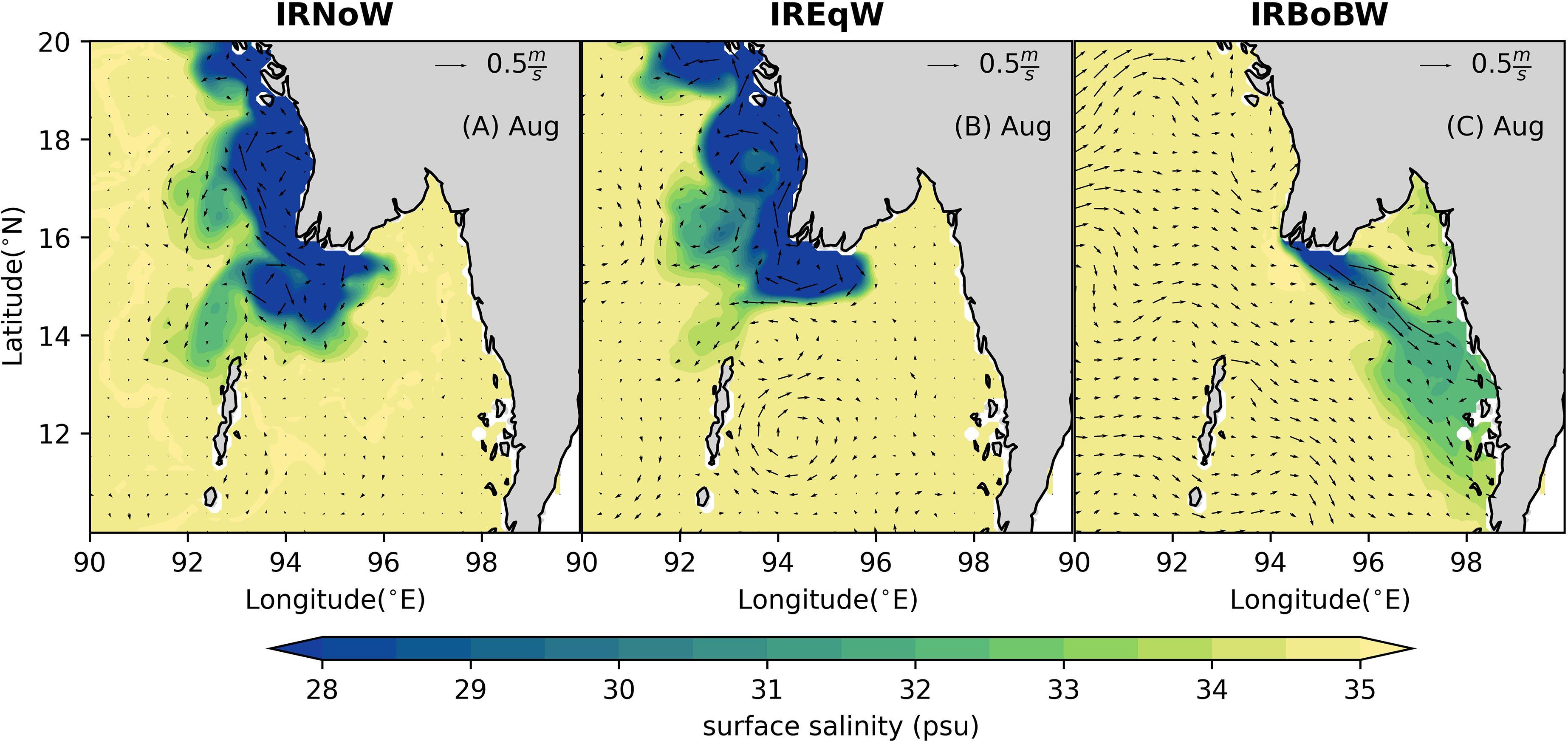
Figure 11 Maps of monthly averaged sea surface salinity(psu) and surface currents(ms^-1) for the month of August from the first year of experiment IRNoW (left), IREqW (center) and IRBoBW (right).

In summary, in the absence of winds, freshwater from IR flows downstream as a coastal current throughout the year. Under the influence of remote forcing, the IR plume flows as a downstream coastal current throughout the year. In both these experiments, the IR plume forms an anticyclonic bulge of freshwater around river mouth and a downstream coastal current which leaks some of the freshwater offshore in the summer monsoon. A comparison of the results from experiments IRFullW and IRBoBW reveals that horizontal structure of the fresh water plume due to the IR is largely controlled by local winds as experiment IRBoBW reproduces the freshwater jet of the IR plume during the summer monsoon. These results show that the density driven flow or the winds over the equator are not the controlling factors of the structure of the IR plume during summer monsoon. They also confirm that the local winds are the most important force contributing to the formation of IR jet in the summer monsoon.

4 Discussion

Wind stress over the study area of IR plume (Andaman Sea) is highest during the peak summer monsoon with southwest-northeast orientation and reverses during winter monsoon. During summer monsoon, the IR plume flows as a narrow band of freshwater towards the shelf in the southeast direction (Figure 4). Analysis of alongshore and cross-shore momentum balance for the month of August reveals that near the river mouth, this southeastward flow occurs completely under the influence of Ekman dynamics (Figure 8). To further confirm that dominant balance throughout the narrow, the southeastward flow of the IR plume is between the Coriolis and wind friction, and we present the vertical distribution of momentum terms across the latitude of 15°N for the month of August from the 6^th year of model integration in experiment IRFullW.

Figure 12 shows that the dominant balance in IR plume is between the Coriolis and wind friction terms. Since the downward penetration of momentum from winds depends upon the vertical stratification of the water column, there is shallower penetration of wind stress where the IR plume is present and this penetration is highlighted by higher values of wind friction term. The figure clearly shows that high stratification caused by the presence of freshwater from IR discharge traps momentum input from winds. Figure 13 shows the distribution of the salinity, density, and u-momentum terms from experiment SpinFullW. Compared to IRFullW, this experiment does not show a high salinity stratification and hence, the trapping of the momentum by a stratified layer. Momentum imparted by winds on highly stratified, highly buoyant water is then balanced by the Coriolis force. The major difference between the two experiments is higher values of density as well as the vertical uniformity in its distribution when the river forcing is absent. However, the capture of momentum in the experiment SpinFullW is significantly less because the vertical density stratification is significantly less. This trapping of momentum imparted by winds in both the horizontal direction by the IR plume during summer monsoon can be clearly seen in the spatial patterns of the wind friction term at the surface from u and v momentum equations (Figure 14). In the Ekman balance, wind stress causes Ekman currents that, at the surface, are orientated at 45° to the right (in northern hemisphere) of wind stress vector. Although winds over the study area during summer monsoon are southwesterly, they have a stronger westerly component. The presence of a stronger westerly wind stress component along with the positive wind friction term in both the horizontal direction as seen in Figure 14, results in southeastward flow of the IR plume during the summer monsoon.

FIGURE 12

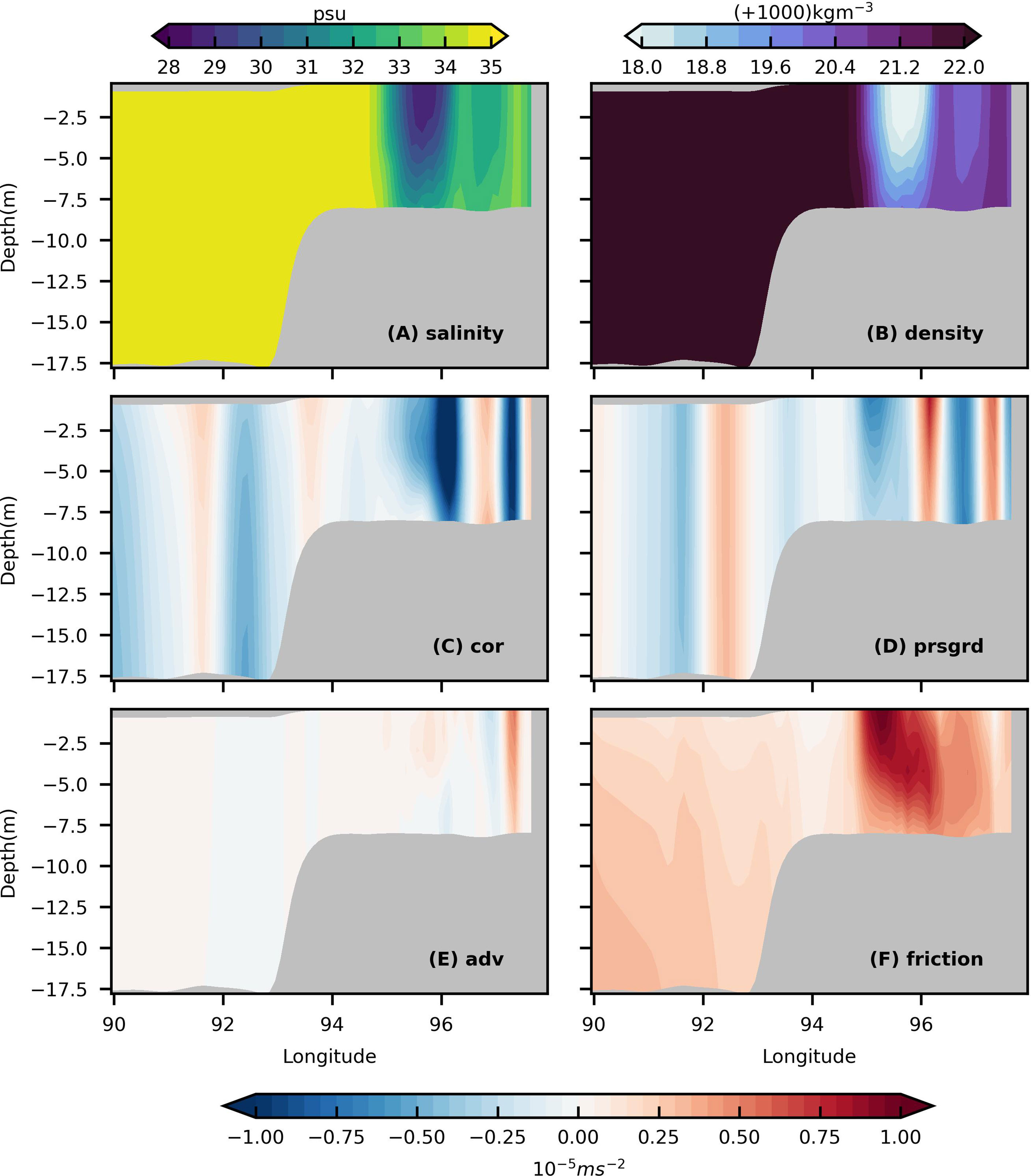
Figure 12 Distribution of (A) salinity, (B) density and (C–F) u-momentum terms from the sixth year of experiment IRFullW for month of August. The distribution presented is across 15°N.

FIGURE 13

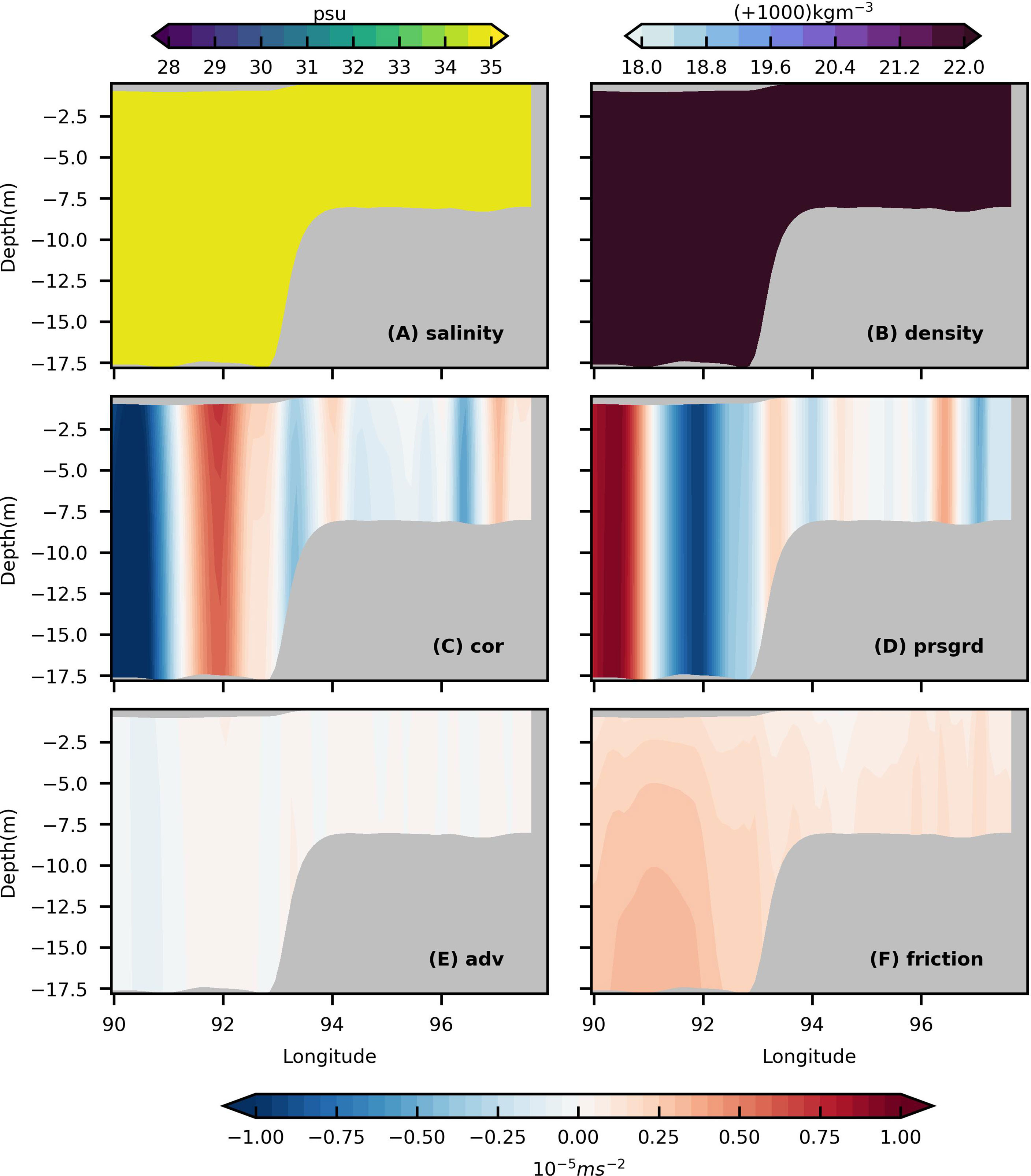
Figure 13 Distribution of (A)salinity, (B)density and (C–F) u-momentum terms from the sixth year of experiment SpinFullW for month of August. The distribution presented is across 15°N.

FIGURE 14

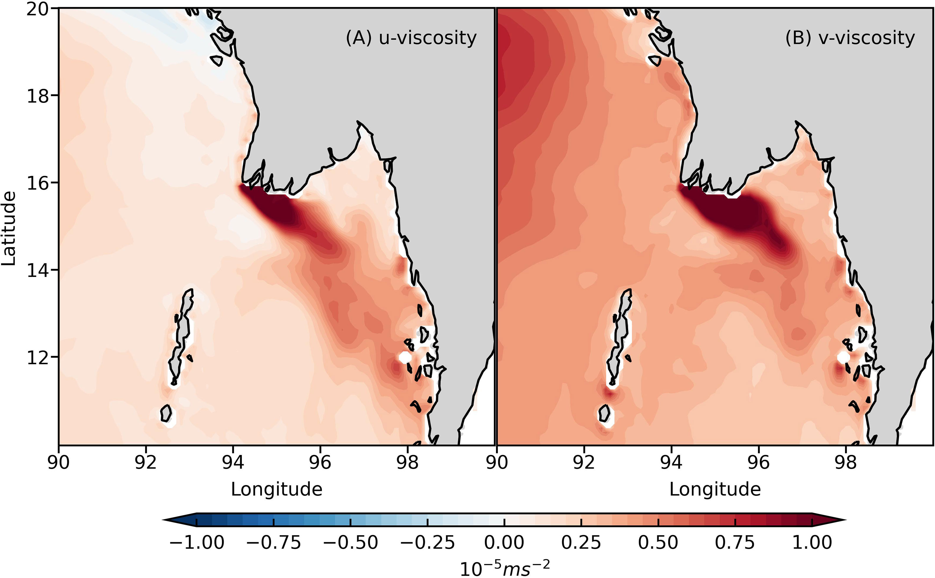
Figure 14 Climatology of wind friction term from (A) u-momentum and (B) v-momentum at the surface in experiment IRFullW during summer monsoon.

As discussed in Section 2.3, there are differences of the order of 2-4 psu between model and observed SSS. This order leads to a large difference of approximately 3 kgm^-3 in the density between the observations and model. A higher density in the model may lead to higher temperatures. However, our model does not show a larger than usual value of temperature as the model SST is relaxed to a climatology. Another reason is that K-Profile Parameterization (KPP) mixing scheme performs reasonably well as it does not produce any erratic values of SST. As observed by Price et al. (1986), a higher temperature (or heating) stratifies and stabilizes the upper layer against shear flow instability caused by winds and enables it to trap heat as well as momentum fluxes from atmosphere. Thus, a surface layer with stronger density stratification traps momentum more easily. They also observed that the heat and momentum fluxes mix in a similar way resulting in velocity and temperature mixed layers with similar thickness. Given same temperature in observations and model (forced by relaxation to climatology), the density stratification in both depends completely on the salinity. A slightly higher density in the model (owing to higher salinity) may result in a slight warming which may further result in stronger stratification in the model as described by Price et al. (1986). This stronger stratification in the model results in stronger currents compared to reanalysis data as shown in Figure 6.

Another quantity which helps us identify the region of momentum trapping by freshwater plume is the surface boundary layer thickness h_sbl. A surface boundary layer is the portion of the ocean directly influenced by the surface forcing/fluxes. In our simulation, surface boundary layer thickness is calculated by K-Profile Parameterization (KPP) vertical mixing scheme of Large et al. (1994). In KPP, surface boundary layer depth is defined as the depth to which the boundary layer eddies with mean velocity and buoyancy equal to the near surface velocity and buoyancy, penetrates, and becomes stable relative to the local velocity and buoyancy. Mathematically, h_sbl is equal to the minimum downward distance z from the surface at which the bulk Richardson number (Ri_b) relative to the surface defined as

$\begin{array}{ll}R{i}_b\left(z\right)=\frac{\left(B_r-B\left(z\right)\right)z}{{\left|u_r-\mathbf{u}\left(\mathbf{z}\right)\right|}^2+V_t^2\left(z\right)}& (3)\end{array}$

reaches a critical value. Here, the reference buoyancy B_r is the buoyancy averaged over the near surface layer in which Monin-Obukhov similarity theory holds and B(z) is the actual buoyancy at z. Similarly, u_r and u(z) are reference and actual vector velocities and V_t represents unresolved turbulent velocity shear. The critical value for Ri_b in our simulations is set to 0.3. Hence, h_sbl is the depth at which

$\begin{array}{ll}R{i}_b\left(h_{sbl}\right)=\frac{\left(B_r-B\left(h_{sbl}\right)\right)h_{sbl}}{{\left|V_r-V\left(h_{sbl}\right)\right|}^2+V_t^2\left(h_{sbl}\right)}=0.3& (4)\end{array}$

Notice that near the surface, Ri_b is zero and increases linearly with depth even if the stabilizing influence of stratification (numerator) is matched by the destabilizing influence of the vertical shear (denominator). In the presence of strong stratification such as the one caused by the presence of freshwater, the buoyancy difference (numerator) is large and hence Ri_b reaches its critical value quickly. This leads to a smaller value of h_sbl. When the stratification is weak, the buoyancy difference is smaller and h_sbl is large. So, under the influence of equal wind forcing conditions, the presence of stronger density stratification (induced by freshwater forcing in our case) gives rise to a shallower surface boundary layer compared to the presence of a weaker density stratification. This presence of shallower surface boundary layer caused by the strong stratification induced by freshwater from the IR can be seen in Figure 15.

FIGURE 15

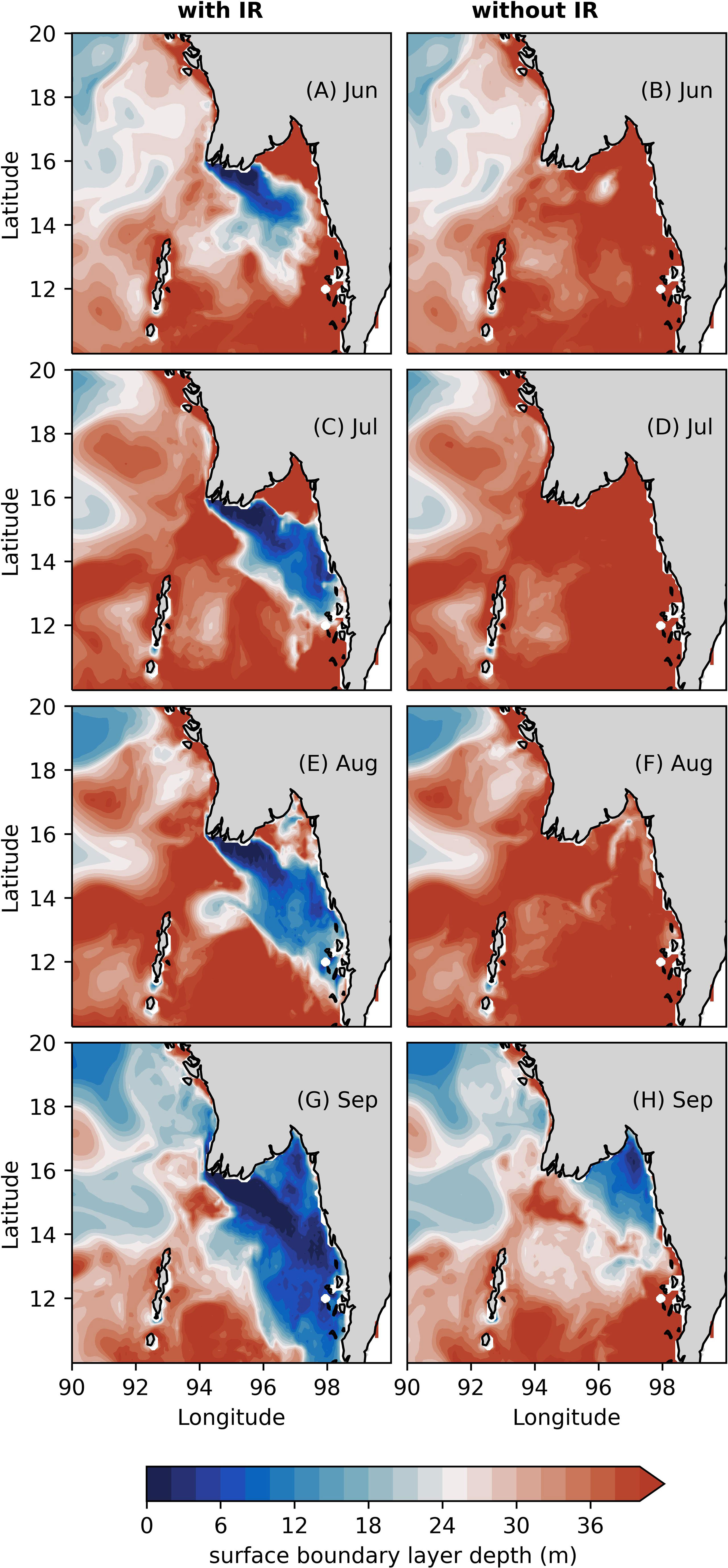
Figure 15 Comparison of the spatial distribution of monthly mean surface boundary layer depth from the first year of experiment IRFullW (first column) and SpinFullW (second column) for the months of summer monsoon.

Figure 15 shows comparison of the spatial distribution of monthly mean surface boundary layer depth (h_sbl) obtained from the first year of experiment IRFullW and SpinFullW for the summer monsoon. As discussed in the Section 3.1, freshwater from the IR flows towards southeast throughout summer monsoon season. A closer inspection of Figures 4, 15 reveals that the spatial distribution of shallower surface boundary layer coincides with the spatial distribution of freshwater from the IR. In the absence of IR freshwater, the surface boundary layer is much deeper (Figures 15E–H).

Shallower surface boundary layer depth also means that the vertical extent of the diffusion of momentum imparted by winds is lesser compared to the deeper surface boundary layer depth and hence, the trapping of momentum in the fewer levels near the surface. This trapping of momentum due to strong density stratification and the deeper extent of momentum diffusion (approximately uniform vertical distribution of wind friction term) in the presence of weaker density stratification can be clearly seen in Figures 12, 13, respectively.

A comparison of spatial distribution of surface salinity from the first year of experiment IRFullW and the wind friction term at the surface from both u and v momentum equation for the summer monsoon season reveals that the higher values of wind friction term are present where the surface salinity is lower (not shown here). Similarly, lower values of surface boundary layer thickness (h_sbl) can be seen where the surface salinity is low (Figures 4A–D, 15A-D). This presence of higher wind friction and lower surface boundary layer thickness in the region of lower salinity (caused by IR freshwater discharge) shows that the presence of freshwater from the IR is necessary to focus momentum input from the wind to drive a jet like structure of the IR plume during the summer monsoon. Presence of freshwater from the IR causes strong density stratification which causes momentum input from winds to diffuse to a lower extent (lower h_sbl) and thus, most of the momentum input is distributed in a smaller region near the surface. This lighter, more buoyant water with higher momentum is then acted upon by the Coriolis force (Ekman balance) to cause a stronger current in the direction perpendicular to the momentum input. This balance between wind friction and the Coriolis term gives rise to a faster flow of IR plume towards southeast during the summer monsoon, as seen in Figure 4.

Experiments conducted using the model also provide insights into the response of the IR plume to different scenarios of wind forcing which have been shown to be significant in driving the circulation in the study area. In the absence of winds, the IR plume flows downstream (northward along the coast of Myanmar). Previous numerical studies show that in the absence of wind forcing, river discharge forms a bulge with anticyclonic circulation just outside the river mouth (Oey and Mellor, 1993; Kourafalou et al., 1996; Fong, 1998; Garvine, 2001; Yankovsky et al., 2001; Fong and Geyer, 2002; Garcia Berdeal et al., 2002; Denamiel et al., 2013). The bulge has also been observed in laboratory experiments (Avicola and Huq, 2002; Horner-Devine et al., 2006) and in the observations (Chant et al., 2008; Horner-Devine, 2009). In our solution without winds (IRNoW), the bulge with anticyclonic circulation forms in the summer monsoon (Figure 11A). Under the influence of equatorial wind forcing, the IR plume flows downstream along the coast of India. The solution IRBoBW (winds over only Bay of Bengal) is a close match to the solution IRFullW indicating a larger influence of local winds over the dynamics of the IR plume.

5 Summary

The characteristics of the Irrawaddy (IR) river plume during summer monsoon are presented in this chapter in an idealized setting wherein the effects of other rivers and rainfall in the study area (consisting of Andaman Sea and northeastern part of Bay of Bengal) are not considered. This approach enables us to isolate the effects of the discharge on salinity structure in the Andaman Sea. Four different experiments, each with a unique wind forcing scenario, were carried out to understand the response of the IR plume to these wind forcing scenarios. These wind forcing scenarios involve winds all over the model domain, no winds, winds only over the equatorial region of the domain, and winds only over the Bay of Bengal region of the domain.

Results presented here reveal that during the summer monsoon, when strong, southwesterly winds prevail over the study area, the IR plume flows towards southeast as a jet and carries most of the discharge to the shelf along the eastern coastline. There are indications of the presence of such a jet in the satellite derived chlorophyll-a data. Reanalysis data from a global ocean model (NEMO) also indicates the presence of the IR jet during the summer monsoon in the Andaman Sea. After reaching the coast, most of the freshwater on the shelf flows southwards along the coast, some flows northward to occupy the southern coast of Myanmar east of the IR mouth. Freshwater reaches as far south as 10°N along the eastern shelf at the end of summer monsoon. The time evolution of the surface salinity, currents, and wind stress show that the momentum input from the winds is trapped by the IR freshwater. Analysis of the momentum balances near the river mouth, as well as inside the plume, confirm that the IR jet is driven by the winds. The orientation of the IR jet is the result of the southwesterly orientation of the winds during the summer monsoon. Model experiments in the absence of winds reveal that the IR plume forms an anticyclonic bulge of freshwater around the river mouth and downstream current. A similar structure is exhibited by the IR plume when only equatorial forcing is present. In the case of winds over Bay of Bengal only, IR plume response is similar to that in experiment IRFullW thus, indicating stronger influence of local winds over horizontal plume structure.

The seasonal orientation of the IR plume, as well as the mechanisms that affect it, have not been reported to date and that makes this study a first of its kind. This study gives a first assessment of the IR plume dynamics and the mechanisms underlying it during the summer monsoon. Results obtained from this study are highly relevant in our understanding of the salinity structure of one of the least studied regions of the Indian Ocean.

Data Availability Statement

The raw data supporting the conclusions of this article will be made available by the authors, without undue reservation.

Author Contributions

SP set up the numerical model and conducted numerical experiments described in this article. SP and PV conceptualized the design of numerical experiments. SP analyzed the output of the numerical experiments and prepared the manuscript. PV assisted in the organization of the results presented in the manuscript. PV reviewed the mansucript and suggested edits for improvement. All authors contributed to the article and approved the submitted version.

Conflict of Interest

The authors declare that the research was conducted in the absence of any commercial or financial relationships that could be construed as a potential conflict of interest.

Publisher’s Note

All claims expressed in this article are solely those of the authors and do not necessarily represent those of their affiliated organizations, or those of the publisher, the editors and the reviewers. Any product that may be evaluated in this article, or claim that may be made by its manufacturer, is not guaranteed or endorsed by the publisher.

Acknowledgments

Partial financial support from J. C. Bose fellowship, SERB, DST, Govt. of India, National Supercomputing Mission (DST & DeitY), Govt of India, and Institute of Eminence grant, IISc, is gratefully acknowledged. ERA-Interim reanalysis surface forcing was provided by European Centre for Medium-Range Weather Forecasts https://www.ecmwf.int. Numerical code employed for the simulations in this study was obtained from Regional Ocean Modeling System website (http://www.myroms.org). Monthly climatology of the chlorophyll-a concentration was obtained from https://modis.gsfc.nasa.gov/data/dataprod/chlor_a.php. Surface currents from global ocean reanalysis (GLOBAL-REANALYSISPHY-001-030) were provided by Copernicus Marine Services (https://marine.copernicus.eu/) and were obtained from https://resources.marine.copernicus.eu/?option=com_csw&view=details&product_id=GLOAL_REANALYSIS_PHY_001_030. Numerical simulations were performed on SAHASRAT, a High Performance Computing system at the Supercomputer Education and Research Centre, IISc. We are thankful to the two anonymous reviewers for their comments and suggestions which improved the presentation of the paper.

References

Akhil V. P., Durand F., Lengaigne M., Vialard J., Keerthi M. G., Gopalakrishna V. V., et al. (2014). A Modeling Study of the Processes of Surface Salinity Seasonal Cycle in the Bay of Bengal. J. Geophys. Res.: Ocean. 119, 3926–3947. doi: 10.1002/2013JC009632

CrossRef Full Text | Google Scholar

Akhil V. P., Lengaigne M., Durand F., Vialard J., Chaitanya A. V. S., Keerthi M. G., et al. (2016a). Assessment of Seasonal and Year-to-Year Surface Salinity Signals Retrieved From SMOS and Aquarius Missions in the Bay of Bengal. Int. J. Remote Sens. 37, 1089–1114. doi: 10.1080/01431161.2016.1145362

CrossRef Full Text | Google Scholar

Akhil V. P., Lengaigne M., Vialard J., Durand F., Keerthi M. G., Chaitanya A. V. S., et al. (2016b). A Modeling Study of Processes Controlling the Bay of Bengal Sea Surface Salinity Interannual Variability. J. Geophys. Res.: Ocean. 121, 8471–8495. doi: 10.1002/2016JC011662

CrossRef Full Text | Google Scholar

Akhil V. P., Vialard J., Lengaigne M., Keerthi M. G., Boutin J., Vergely J.-L., et al. (2020). Bay of Bengal Sea Surface Salinity Variability Using a Decade of Improved SMOS Re-Processing. Remote Sens. Environ. 248, 111964. doi: 10.1016/j.rse.2020.111964

CrossRef Full Text | Google Scholar

Alpers W., Wang-Chen H., Hock L. (1997). “Observation of Internal Waves in the Andaman Sea by ERS SAR. In Igarss’97,” in 1997 IEEE International Geoscience and Remote Sensing Symposium Proceedings. Remote Sensing-A Scientific Vision for Sustainable Development, vol. 4. (Singapore: IEEE), 1518–1520.

Google Scholar

Androulidakis Y. S., Kourafalou V. H., Schiller R. V. (2015). Process Studies on the Evolution of the Mississippi River Plume: Impact of Topography, Wind and Discharge Conditions. Continent. Shelf. Res. 107, 33–49. doi: 10.1016/j.csr.2015.07.014

CrossRef Full Text | Google Scholar

Antonov J., Seidov D., Boyer T., Locarnini R., Mishonov A., Garcia H., et al. (2010). World Ocean Atlas 2009, Volume 2: Salinity. Ed. Levitus S. (Printing Office, Washington, D.C.: NOAA Atlas NESDIS 69), 184.

Google Scholar

Ashin K., Girishkumar M., Suprit K., Thangaprakash V. (2019). Observed Upper Ocean Seasonal and Intraseasonal Variability in the Andaman Sea. J. Geophys. Res.: Ocean. 124, 6760–6786. doi: 10.1029/2019JC014938

CrossRef Full Text | Google Scholar

Avicola G., Huq P. (2002). Scaling Analysis for the Interaction Between a Buoyant Coastal Current and the Continental Shelf: Experiments and Observations. J. Phys. Oceanogr. 32, 3233–3248. doi: 10.1175/1520-0485(2002)032<3233:SAFTIB>2.0.CO;2

CrossRef Full Text | Google Scholar

Avicola G., Huq P. (2003a). The Characteristics of the Recirculating Bulge Region in Coastal Buoyant Outflows. J. Mar. Res. 61, 435–463. doi: 10.1357/002224003322384889

CrossRef Full Text | Google Scholar

Avicola G., Huq P. (2003b). The Role of Outflow Geometry in the Formation of the Recirculating Bulge Region in Coastal Buoyant Outflows. J. Mar. Res. 61, 411–434. doi: 10.1357/002224003322384870

CrossRef Full Text | Google Scholar

Baronas J. J., Stevenson E. I., Hackney C. R., Darby S. E., Bickle M. J., Hilton R. G., et al. (2020). Integrating Suspended Sediment Flux in Large Alluvial River Channels: Application of a Synoptic Rouse-Based Model to the Irrawaddy and Salween Rivers. J. Geophys. Res.: Earth Surf. 125, e2020JF005554. doi: 10.1029/2020JF005554

CrossRef Full Text | Google Scholar

Behara A., Vinayachandran P. (2016). An OGCM Study of the Impact of Rain and River Water Forcing on the Bay of Bengal. J. Geophys. Res.: Ocean. 121, 2425–2446. doi: 10.1002/2015JC011325

CrossRef Full Text | Google Scholar

Benshila R., Durand F., Masson S., Bourdallé-Badie R., de Boyer Montégut C., Papa F., et al. (2014). The Upper Bay of Bengal Salinity Structure in a High-Resolution Model. Ocean. Modell. 74, 36–52. doi: 10.1016/j.ocemod.2013.12.001

CrossRef Full Text | Google Scholar

Chandran S. T., Raj S. B., Ravindran S., Narayana S. V. (2018). Upper Layer Circulation, Hydrography, and Biological Response of the Andaman Waters During Winter Monsoon Based on in Situ and Satellite Observations. Ocean. Dynam. 68, 801–815. doi: 10.1007/s10236-018-1160-x

CrossRef Full Text | Google Scholar

Chant R. J., Glenn S. M., Hunter E., Kohut J., Chen R. F., Houghton R. W., et al. (2008). Bulge Formation of a Buoyant River Outflow. J. Geophys. Res.: Ocean. 113, C01017. doi: 10.1029/2007JC004100

CrossRef Full Text | Google Scholar

Chao S.-Y. (1988). Wind-Driven Motion of Estuarine Plumes. J. Phys. Oceanogr. 18, 1144–1166. doi: 10.1175/1520-0485(1988)018<1144:WDMOEP>2.0.CO;2

CrossRef Full Text | Google Scholar

Chao S.-Y., Boicourt W. C. (1986). Onset of Estuarine Plumes. J. Phys. Oceanogr. 16, 2137–2149. doi: 10.1175/1520-0485(1986)016<2137:OOEP>2.0.CO;2

CrossRef Full Text | Google Scholar

Chatterjee A., Shankar D., McCreary J., Vinayachandran P., Mukherjee A. (2017). Dynamics of Andaman Sea Circulation and its Role in Connecting the Equatorial Indian Ocean to the Bay of Bengal. J. Geophys. Res.: Ocean. 122, 3200–3218. doi: 10.1002/2016JC012300

CrossRef Full Text | Google Scholar

Chaudhuri D., Sengupta D., D’Asaro E., Shivaprasad S. (2021). Trapping of Wind Momentum in a Salinity-Stratified Ocean. J. Geophys. Res.: Ocean. 126, e2021JC017770. doi: 10.1029/2021JC017770

CrossRef Full Text | Google Scholar

Cheng X., Xie S.-P., McCreary J. P., Qi Y., Du Y. (2013). Intraseasonal Variability of Sea Surface Height in the Bay of Bengal. J. Geophys. Res.: Ocean. 118, 816–830. doi: 10.1002/jgrc.20075

CrossRef Full Text | Google Scholar

Choi B.-J., Wilkin J. L. (2007). The Effect of Wind on the Dispersal of the Hudson River Plume. J. Phys. Oceanogr. 37, 1878–1897. doi: 10.1175/JPO3081.1

CrossRef Full Text | Google Scholar

Dai A., Qian T., Trenberth K. E., Milliman J. D. (2009). Changes in Continental Freshwater Discharge From 1948 to 2004. J. Climate 22, 2773–2792. doi: 10.1175/2008JCLI2592.1

CrossRef Full Text | Google Scholar

Dai A., Trenberth K. E. (2002). Estimates of Freshwater Discharge From Continents: Latitudinal and Seasonal Variations. J. Hydrometeorol. 3, 660–687. doi: 10.1175/1525-7541(2002)003<0660:EOFDFC>2.0.CO;2

CrossRef Full Text | Google Scholar

Dee D. P., Uppala S. M., Simmons A., Berrisford P., Poli P., Kobayashi S., et al. (2011). The ERA-Interim Reanalysis: Configuration and Performance of the Data Assimilation System. Q. J. R. Meteorol. Soc. 137, 553–597. doi: 10.1002/qj.828

CrossRef Full Text | Google Scholar

Denamiel C., Budgell W. P., Toumi R. (2013). The Congo River Plume: Impact of the Forcing on the Far-Field and Near-Field Dynamics. J. Geophys. Res.: Ocean. 118, 964–989. doi: 10.1002/jgrc.20062

CrossRef Full Text | Google Scholar

Ferry N., Barnier B., Garric G., Haines K., Masina S., Parent L., et al. (2012). NEMO: The Modeling Engine of Global Ocean Reanalyses. Merc. Ocean. Q. Newslett. 46, 46–59.

Google Scholar

Fong D. A. (1998). “Dynamics of Freshwater Plumes: Observations and Numerical Modeling of the Wind-Forced Response and Alongshore Freshwater Transport. Ph.D. Thesis,” in Massachusetts Institute of Technology and Woods Hole Oceanographic Institution. (Cambridge, MA).

Google Scholar

Fong D. A., Geyer W. R. (2002). The Alongshore Transport of Freshwater in a Surface-Trapped River Plume. J. Phys. Oceanogr. 32, 957–972. doi: 10.1175/1520-0485(2002)032<0957:TATOFI>2.0.CO;2

CrossRef Full Text | Google Scholar

Fore A. G., Yueh S. H., Tang W., Stiles B. W., Hayashi A. K. (2016). Combined Active/Passive Retrievals of Ocean Vector Wind and Sea Surface Salinity With SMAP. IEEE Trans. Geosci. Remote Sens. 54, 7396–7404. doi: 10.1109/TGRS.2016.2601486

CrossRef Full Text | Google Scholar

Garcia Berdeal I., Hickey B., Kawase M. (2002). Influence of Wind Stress and Ambient Flow on a High Discharge River Plume. J. Geophys. Res.: Ocean. 107, 13–11. doi: 10.1029/2001JC000932

CrossRef Full Text | Google Scholar

Garvine R. W. (1987). Estuary Plumes and Fronts in Shelf Waters: A Layer Model. J. Phys. Oceanogr. 17, 1877–1896. doi: 10.1175/1520-0485(1987)017<1877:EPAFIS>2.0.CO;2

CrossRef Full Text | Google Scholar

Garvine R. W. (1999). Penetration of Buoyant Coastal Discharge Onto the Continental Shelf: A Numerical Model Experiment. J. Phys. Oceanogr. 29, 1892–1909. doi: 10.1175/1520-0485(1999)029<1892:POBCDO>2.0.CO;2

CrossRef Full Text | Google Scholar

Garvine R. W. (2001). The Impact of Model Configuration in Studies of Buoyant Coastal Discharge. J. Mar. Res. 59, 193–225. doi: 10.1357/002224001762882637

CrossRef Full Text | Google Scholar

Gordon A. L., Shroyer E. L., Mahadevan A., Sengupta D., Freilich M. (2016). Bay of Bengal: 2013 Northeast Monsoon Upper-Ocean Circulation. Oceanography 29, 82–91. doi: 10.5670/oceanog.2016.41

CrossRef Full Text | Google Scholar

Greaser S. R., Subrahmanyam B., Trott C. B., Roman-Stork H. L. (2020). Interactions Between Mesoscale Eddies and Synoptic Oscillations in the Bay of Bengal During the Strong Monsoon of 2019. J. Geophys. Res.: Ocean. 125, e2020JC016772. doi: 10.1029/2020JC016772

CrossRef Full Text | Google Scholar

Haidvogel D. B., Arango H. G., Hedstrom K., Beckmann A., Malanotte-Rizzoli P., Shchepetkin A. F. (2000). Model Evaluation Experiments in the North Atlantic Basin: Simulations in Nonlinear Terrain-Following Coordinates. Dynam. Atmosph. Ocean. 32, 239–281. doi: 10.1016/S0377-0265(00)00049-X

CrossRef Full Text | Google Scholar

Han W., McCreary J. P. (2001). Modeling Salinity Distributions in the Indian Ocean. J. Geophys. Res.: Ocean. 106, 859–877. doi: 10.1029/2000JC000316

CrossRef Full Text | Google Scholar

Hetland R. D. (2005). Relating River Plume Structure to Vertical Mixing. J. Phys. Oceanogr. 35, 1667–1688. doi: 10.1175/JPO2774.1

CrossRef Full Text | Google Scholar

Hormann V., Centurioni L. R., Gordon A. L. (2019). Freshwater Export Pathways From the Bay of Bengal. Deep. Sea. Res. Part II.: Top. Stud. Oceanogr. 168, 104645. doi: 10.1016/j.dsr2.2019.104645

CrossRef Full Text | Google Scholar

Horner-Devine A. R. (2009). The Bulge Circulation in the Columbia River Plume. Continent. Shelf. Res. 29, 234–251. doi: 10.1016/j.csr.2007.12.012

CrossRef Full Text | Google Scholar

Horner-Devine A. R., Fong D. A., Monismith S. G., Maxworthy T. (2006). Laboratory Experiments Simulating a Coastal River Inflow. J. Fluid. Mech. 555, 203–232. doi: 10.1017/S0022112006008937

CrossRef Full Text | Google Scholar

Howden S. D., Murtugudde R. (2001). Effects of River Inputs Into the Bay of Bengal. J. Geophys. Res.: Ocean. 106, 19825–19843. doi: 10.1029/2000JC000656

CrossRef Full Text | Google Scholar

Hyder P., Jeans D., Cauquil E., Nerzic R. (2005). Observations and Predictability of Internal Solitons in the Northern Andaman Sea. Appl. Ocean. Res. 27, 1–11. doi: 10.1016/j.apor.2005.07.001

CrossRef Full Text | Google Scholar

Ikeda M. (1984). Coastal Flows Driven by a Local Density Flux. J. Geophys. Res.: Ocean. 89, 8008–8016. doi: 10.1029/JC089iC05p08008

CrossRef Full Text | Google Scholar

Jana S., Gangopadhyay A., Chakraborty A. (2015). Impact of Seasonal River Input on the Bay of Bengal Simulation. Continent. Shelf. Res. 104, 45–62. doi: 10.1016/j.csr.2015.05.001

CrossRef Full Text | Google Scholar

Janzen C. D., Wong K.-C. (2002). Wind-Forced Dynamics at the Estuary-Shelf Interface of a Large Coastal Plain Estuary. J. Geophys. Res.: Ocean. 107, 2–1. doi: 10.1029/2001JC000959

CrossRef Full Text | Google Scholar

Jensen T. G. (2001). Arabian Sea and Bay of Bengal Exchange of Salt and Tracers in an Ocean Model. Geophys. Res. Lett. 28, 3967–3970. doi: 10.1029/2001GL013422

CrossRef Full Text | Google Scholar

Jensen T. G., Wijesekera H. W., Nyadjro E. S., Thoppil P. G., Shriver J. F., Sandeep K., et al. (2016). Modeling Salinity Exchanges Between the Equatorial Indian Ocean and the Bay of Bengal. Oceanography 29, 92–101. doi: 10.5670/oceanog.2016.42

CrossRef Full Text | Google Scholar

Jithin A., Francis P. (2020). Role of Internal Tide Mixing in Keeping the Deep Andaman Sea Warmer Than the Bay of Bengal. Sci. Rep. 10, 1–10. doi: 10.1038/s41598-020-68708-6

PubMed Abstract | CrossRef Full Text | Google Scholar

Kao T. W. (1981). The Dynamics of Oceanic Fronts. Part II: Shelf Water Structure Due to Freshwater Discharge. J. Phys. Oceanogr. 11, 1215–1223. doi: 10.1175/1520-0485(1981)011<1215:TDOOFP>2.0.CO;2

CrossRef Full Text | Google Scholar

Kao T. W., Park C., Pao H.-P. (1977). Buoyant Surface Discharge and Small-Scale Oceanic Fronts: A Numerical Study. J. Geophys. Res. 82, 1747–1752. doi: 10.1029/JC082i012p01747

CrossRef Full Text | Google Scholar

Kastner S. E., Horner-Devine A. R., Thomson J. (2018). The Influence of Wind and Waves on Spreading and Mixing in the Fraser River Plume. J. Geophys. Res.: Ocean. 123, 6818–6840. doi: 10.1029/2018JC013765

CrossRef Full Text | Google Scholar

Kourafalou V. H., Oey L.-Y., Wang J. D., Lee T. N. (1996). The Fate of River Discharge on the Continental Shelf: 1. Modeling the River Plume and the Inner Shelf Coastal Current. J. Geophys. Res.: Ocean. 101, 3415–3434. doi: 10.1029/95JC03024

CrossRef Full Text | Google Scholar

Kumari A., Kumar S. P., Chakraborty A. (2018). Seasonal and Interannual Variability in the Barrier Layer of the Bay of Bengal. J. Geophys. Res.: Ocean. 123, 1001–1015. doi: 10.1002/2017JC013213

CrossRef Full Text | Google Scholar

Large W. G., McWilliams J. C., Doney S. C. (1994). Oceanic Vertical Mixing: A Review and a Model With a Nonlocal Boundary Layer Parameterization. Rev. Geophys. 32, 363–403. doi: 10.1029/94RG01872

CrossRef Full Text | Google Scholar

Lentz S. (2004). The Response of Buoyant Coastal Plumes to Upwelling-Favorable Winds. J. Phys. Oceanogr. 34, 2458–2469. doi: 10.1175/JPO2647.1

CrossRef Full Text | Google Scholar

Lentz S. J., Largier J. (2006). The Influence of Wind Forcing on the Chesapeake Bay Buoyant Coastal Current. J. Phys. Oceanogr. 36, 1305–1316. doi: 10.1175/JPO2909.1

CrossRef Full Text | Google Scholar

Liu Y., Li K., Ning C., Yang Y., Wang H., Liu J., et al. (2018). Observed Seasonal Variations of the Upper Ocean Structure and Air-Sea Interactions in the Andaman Sea. J. Geophys. Res.: Ocean. 123, 922–938. doi: 10.1002/2017JC013367

CrossRef Full Text | Google Scholar

Madec G., Team (2019). NEMO Ocean Engine. Sci. Notes Climate Modell. Center. doi: 10.5281/zenodo.1464816

CrossRef Full Text | Google Scholar

Mazzini P. L. F., Chant R. J., Scully M., Wilkin J., Hunter E., Nidzieko N. (2019). The Impact of Wind Forcing on the Thermal Wind Shear of a River Plume. J. Geophys. Res.: Ocean. 124, 7908–7925. doi: 10.1029/2019JC015259

CrossRef Full Text | Google Scholar

McCreary H. ,. W., Shankar D., Shetye S. (1996). Dynamics of the East India Coastal Current: 2. Numerical Solutions. J. Geophys. Res.: Ocean. 101, 13993–14010. doi: 10.1029/96JC00560

CrossRef Full Text | Google Scholar

Milliman J. D., Farnsworth K. L. (2013). River Discharge to the Coastal Ocean: A Global Synthesis (Cambridge: Cambridge University Press).

Google Scholar

Momin I. M., Mitra A., Bhatla R. (2021). Assessment of NEMO Simulated Surface Current With HF Radar Along Andhra Pradesh Coast. J. Earth Syst. Sci. 130, 1–11. doi: 10.1007/s12040-021-01553-x

CrossRef Full Text | Google Scholar

Oey L.-Y., Mellor G. (1993). Subtidal Variability of Estuarine Outflow, Plume, and Coastal Current: A Model Study. J. Phys. Oceanogr. 23, 164–171. doi: 10.1175/1520-0485(1993)023<0164:SVOEOP>2.0.CO;2

CrossRef Full Text | Google Scholar

Osborne A., Burch T. (1980). Internal Solitons in the Andaman Sea. Science 208, 451–460. doi: 10.1126/science.208.4443.451

PubMed Abstract | CrossRef Full Text | Google Scholar

Pant V., Girishkumar M., Udaya Bhaskar T., Ravichandran M., Papa F., Thangaprakash V. (2015). Observed Interannual Variability of Near-Surface Salinity in the Bay of Bengal. J. Geophys. Res.: Ocean. 120, 3315–3329. doi: 10.1002/2014JC010340

CrossRef Full Text | Google Scholar

Pargaonkar S. M., Vinayachandran P. (2021). Wind Forcing of the Ganga-Brahmaputra River Plume. Ocean. Dynam. 71, 125–156. doi: 10.1007/s10236-020-01429-6

CrossRef Full Text | Google Scholar

Pimenta F. M., Kirwan A. Jr. (2014). The Response of Large Outflows to Wind Forcing. Continent. Shelf. Res. 89, 24–37. doi: 10.1016/j.csr.2013.11.006

CrossRef Full Text | Google Scholar

Potemra J. T., Luther M. E., O’Brien J. J. (1991). The Seasonal Circulation of the Upper Ocean in the Bay of Bengal. J. Geophys. Res.: Ocean. 96, 12667–12683. doi: 10.1029/91JC01045

CrossRef Full Text | Google Scholar

Price J. F., Weller R. A., Pinkel R. (1986). Diurnal Cycling: Observations and Models of the Upper Ocean Response to Diurnal Heating, Cooling, and Wind Mixing. J. Geophys. Res.: Ocean. 91, 8411–8427. doi: 10.1029/JC091iC07p08411

CrossRef Full Text | Google Scholar

Pullen J. D., Allen J. (2000). Modeling Studies of the Coastal Circulation Off Northern California: Shelf Response to a Major Eel River Flood Event. Continent. Shelf. Res. 20, 2213–2238. doi: 10.1016/S0278-4343(00)00068-6

CrossRef Full Text | Google Scholar

Qi L., Wang Y. (2015). Discrepancies in Different Precipitation Data Products in the Bay of Bengal During Summer Monsoon Season. Adv. Meteorol. 2015, C06029. doi: 10.1155/2015/806845

CrossRef Full Text | Google Scholar

Sanchez-Franks A., Webber B., King B., Vinayachandran P., Matthews A., Sheehan P. M., et al. (2019). The Railroad Switch Effect of Seasonally Reversing Currents on the Bay of Bengal High-Salinity Core. Geophys. Res. Lett. 46, 6005–6014. doi: 10.1029/2019GL082208

CrossRef Full Text | Google Scholar

Schiller R., Kourafalou V., Hogan P., Walker N. (2011). The Dynamics of the Mississippi River Plume: Impact of Topography, Wind and Offshore Forcing on the Fate of Plume Waters. J. Geophys. Res.: Ocean. 116. doi: 10.1029/2010JC006883

CrossRef Full Text | Google Scholar

Sengupta D., Bharath Raj G., Ravichandran M., Sree Lekha J., Papa F. (2016). Near-Surface Salinity and Stratification in the North Bay of Bengal From Moored Observations. Geophys. Res. Lett. 43, 4448–4456. doi: 10.1002/2016GL068339

CrossRef Full Text | Google Scholar

Seo H., Xie S.-P., Murtugudde R., Jochum M., Miller A. J. (2009). Seasonal Effects of Indian Ocean Freshwater Forcing in a Regional Coupled Model. J. Climate 22, 6577–6596. doi: 10.1175/2009JCLI2990.1

CrossRef Full Text | Google Scholar

Shankar D., McCreary J., Han W., Shetye S. (1996). Dynamics of the East India Coastal Current: 1. Analytic Solutions Forced by Interior Ekman Pumping and Local Alongshore Winds. J. Geophys. Res.: Ocean. 101, 13975–13991. doi: 10.1029/96JC00559

CrossRef Full Text | Google Scholar

Shankar D., Vinayachandran P., Unnikrishnan A. (2002). The Monsoon Currents in the North Indian Ocean. Prog. Oceanogr. 52, 63–120. doi: 10.1016/S0079-6611(02)00024-1

CrossRef Full Text | Google Scholar

Sharma R., Agarwal N., Chakraborty A., Mallick S., Buckley J., Shesu V., et al. (2016). Large-Scale Air-Sea Coupling Processes in the Bay Of Bengal Using Space-Borne Observations. Oceanography 29, 192–201. doi: 10.5670/oceanog.2016.51

CrossRef Full Text | Google Scholar

Shchepetkin A. F., McWilliams J. C. (2005). The Regional Oceanic Modeling System (ROMS): A Split-Explicit, Free-Surface, Topography-Following-Coordinate Oceanic Model. Ocean. Modell. 9, 347–404. doi: 10.1016/j.ocemod.2004.08.002

CrossRef Full Text | Google Scholar

Shetye S. R. (1993). The Movement and Implications of the Ganges—Bramhaputra Runoff on Entering the. Curr. Sci. 64, 32–28.

Google Scholar

Shroyer E. L., Gordon A. L., Jaeger G. S., Freilich M., Waterhouse A. F., Farrar J. T., et al. (2020). Upper Layer Thermohaline Structure of the Bay of Bengal During the 2013 Northeast Monsoon. Deep. Sea. Res. Part II.: Top. Stud. Oceanogr. 172, 104630. doi: 10.1016/j.dsr2.2019.07.018

CrossRef Full Text | Google Scholar

Sprintall J., Tomczak M. (1992). Evidence of the Barrier Layer in the Surface Layer of the Tropics. J. Geophys. Res.: Ocean. 97, 7305–7316. doi: 10.1029/92JC00407

CrossRef Full Text | Google Scholar

Trott C. B., Subrahmanyam B., Roman-Stork H. L., Murty V., Gnanaseelan C. (2019). Variability of Intraseasonal Oscillations and Synoptic Signals in Sea Surface Salinity in the Bay of Bengal. J. Climate 32, 6703–6728. doi: 10.1175/JCLI-D-19-0178.1

CrossRef Full Text | Google Scholar

Varkey M., Murty V., Suryanarayana A. (1997). Physical Oceanography of the Bay of Bengal and Andaman Sea. Oceanogr. Literat. Rev. 5, 413.

Google Scholar

Vinayachandran P., Kurian J. (2007). Hydrographic Observations and Model Simulation of the Bay of Bengal Freshwater Plume. Deep. Sea. Res. Part I.: Oceanogr. Res. Paper 54, 471–486. doi: 10.1016/j.dsr.2007.01.007

CrossRef Full Text | Google Scholar

Vinayachandran P., Murty V., Ramesh Babu V. (2002). Observations of Barrier Layer Formation in the Bay of Bengal During Summer Monsoon. J. Geophys. Res.: Ocean. 107, SRF 19.1–SRF 19.9. doi: 10.1029/2001JC000831

CrossRef Full Text | Google Scholar

Vinayachandran P., Nanjundiah R. S. (2009). Indian Ocean Sea Surface Salinity Variations in a Coupled Model. Climate Dynam. 33, 245–263. doi: 10.1007/s00382-008-0511-6

CrossRef Full Text | Google Scholar

Vinayachandran P., Neema C., Mathew S., Remya R. (2012). Mechanisms of Summer Intraseasonal Sea Surface Temperature Oscillations in the Bay of Bengal. J. Geophys. Res.: Ocean. 117, C01005. doi: 10.1029/2011JC007433

CrossRef Full Text | Google Scholar

Vinayachandran P., Shetye S. R., Sengupta D., Gadgil S. (1996). Forcing mechanisms of the Bay of Bengal. Curr. Sci. 70, 753–763.

Google Scholar

Walker N. D., Wiseman W. J. Jr., Rouse L. J. Jr., Babin A. (2005). Effects of River Discharge, Wind Stress, and Slope Eddies on Circulation and the Satellite-Observed Structure of the Mississippi River Plume. J. Coast. Res. 2005, 1228–1244. doi: 10.2112/04-0347.1

CrossRef Full Text | Google Scholar

Webber B. G., Matthews A. J., Vinayachandran P., Neema C., Sanchez-Franks A., Vijith V., et al. (2018). The Dynamics of the Southwest Monsoon Current in 2016 From High-Resolution In Situ Observations and Models. J. Phys. Oceanogr. 48, 2259–2282. doi: 10.1175/JPO-D-17-0215.1

CrossRef Full Text | Google Scholar

Whitney M. M., Garvine R. W. (2006). Simulating the Delaware Bay Buoyant Outflow: Comparison With Observations. J. Phys. Oceanogr. 36, 3–21. doi: 10.1175/JPO2805.1

CrossRef Full Text | Google Scholar

Yankovsky A. E. (2000). The Cyclonic Turning and Propagation of Buoyant Coastal Discharge Along the Shelf. J. Mar. Res. 58, 585–607. doi: 10.1357/002224000321511034

CrossRef Full Text | Google Scholar

Yankovsky A. E., Chapman D. C. (1997). A Simple Theory for the Fate of Buoyant Coastal Discharges. J. Phys. Oceanogr. 27, 1386–1401. doi: 10.1175/1520-0485(1997)027<1386:ASTFTF>2.0.CO;2

CrossRef Full Text | Google Scholar

Yankovsky A. E., Hickey B. M., Münchow A. K. (2001). Impact of Variable Inflow on the Dynamics of a Coastal Buoyant Plume. J. Geophys. Res.: Ocean. 106, 19809–19824. doi: 10.1029/2001JC000792

CrossRef Full Text | Google Scholar

Yu L., O’Brien J. J., Yang J. (1991). On the Remote Forcing of the Circulation in the Bay of Bengal. J. Geophys. Res.: Ocean. 96, 20449–20454. doi: 10.1029/91JC02424

CrossRef Full Text | Google Scholar

Zhang W. G., Wilkin J. L., Chant R. J. (2009). Modeling the Pathways and Mean Dynamics of River Plume Dispersal in the New York Bight. J. Phys. Oceanogr. 39, 1167–1183. doi: 10.1175/2008JPO4082.1

CrossRef Full Text | Google Scholar