Shelf Water Export at the Brazil-Malvinas Confluence Evidenced From Combined in situ and Satellite Observations

Introduction

Western boundary currents (WBCs) and adjacent continental shelves display two distinct circulation regimes separated by a strong vorticity barrier and therefore exhibit distinct water-mass properties and ecosystem composition (Roughan et al., 2011; Franco et al., 2018). Nevertheless, at the separation of WBCs from the shelf-break, the instabilities of the currents generate meanders and eddies that induce strong interactions between the shelf and the deep ocean generating intense cross-shelf exchanges (Arruda and da Silveira, 2019; Ismail and Ribbe, 2019; Malan et al., 2020; Roughan et al., 2022). These cross-shelf exchanges have important consequences for marine life, as they provide nutrients to the oligotrophic deep ocean and offshore advection of larvae from species that live on the shelf (Franco et al., 2017, 2018). Historically, these systems have been difficult to model accurately, due to a combination of numerical constraints such as small-scale highly energetic dynamics over steep and complex topography, and also due to the lack of observations to compare with, making the sampling of these sporadic events very valuable.

In the South Atlantic, the WBCs are the poleward flowing warm and salty south Brazil Current (BC), which is a relatively weak western boundary current associated with the subtropical gyre, and the cold and relatively fresh northward-flowing Malvinas Current (MC), which is a branch of the Antarctic Circumpolar Current (Gordon, 1989). While the BC extends down to about 500 m, the MC presents a predominantly barotropic structure and extends to the bottom (e.g., Vivier and Provost, 1999). Both currents converge along the South American slope at about 38°S at the so-called Brazil-Malvinas Confluence (BMC), generating one of the most energetic mesoscale regions of the global ocean (Chelton et al., 1990). On average, the BC begins to separate from the shelf break at 36.5°S, and the main core of the MC retroflects at about 38.8°S where the 200 and 1,000 m isobaths diverge at Ewing terrace. At that point, the MC is no longer constrained by the topographic steering and retroflects, while a shallow branch of the MC continues northward over the shelf-break (Matano et al., 2010). Between 36.5 and 38.8°S, the ocean area over the slope is characterized by high eddy kinetic energy with changes in current speed and direction (Figure 1A). Satellite-derived salinity, in situ observations, and modeling studies suggest that this region is also where most of the cross-shelf exchanges in the Southwestern Atlantic take place (Guerrero et al., 2014; Matano et al., 2014; Franco et al., 2018; Berden et al., 2020; Orúe-Echevarría et al., 2021).

FIGURE 1

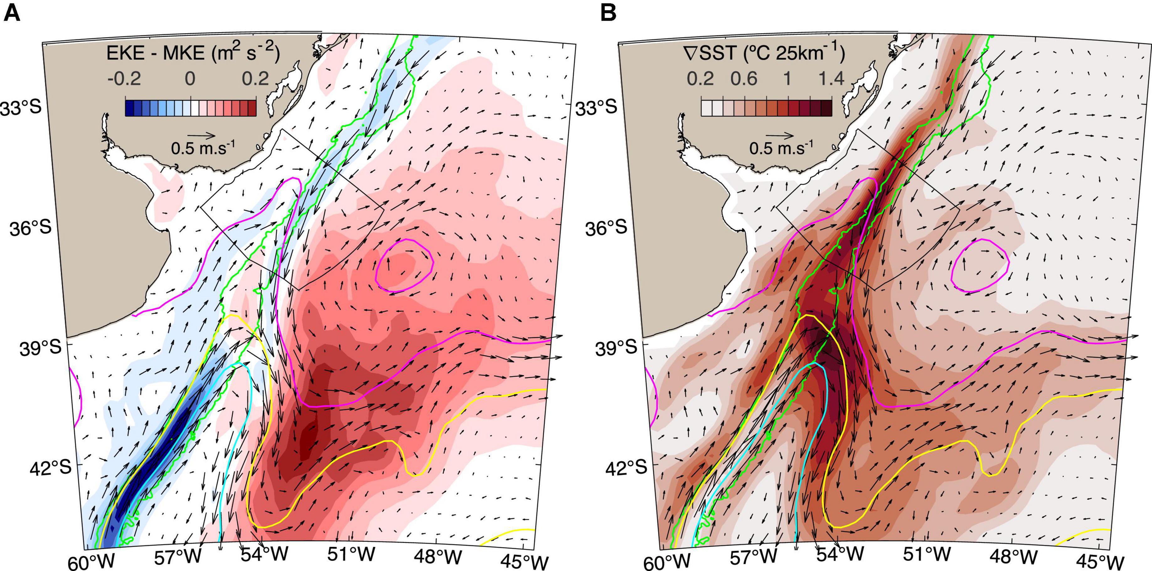
Figure 1. Long-term mean conditions in the Southwestern Atlantic Ocean derived from satellite observations. Both panels show the mean surface geostrophic currents displayed as black arrows, the green lines show the 500 and 2,500 m isobaths, and the 0 m (cyan), 0.25 m (yellow), and 0.5 m (magenta) Absolute Dynamic Topography contours which indicate the retroflection of the main core of the Malvinas Current, the mean confluence position and the separation of the Brazil Current from the shelf-break, respectively. The black polygon delimits the Uruguayan Exclusive Economic Zone (EEZ). Background colors show the long-term daily mean of (A) eddy kinetic energy (EKE) minus mean kinetic energy (MKE) and (B) SST gradient.

The Uruguayan Economic Exclusive Zone (EEZ) is located in the northwestern edge of the Argentine Basin covering the slope between 34.6 and 37.3°S. The EEZ spans an area of about 140 × 10³ km² (Figure 1) and includes part of the region of high kinetic energy and intense cross-shelf exchanges (e.g., Guerrero et al., 2014; Matano et al., 2014; Franco et al., 2018; Berden et al., 2020). The water column over the slope region is characterized by at least six water masses from various sources, a micro-tidal regime, and large seasonal variability. Sea surface temperature (SST) variability presents a seasonal amplitude of 12°C and the wind stress curl reverses seasonally (Piola et al., 2018). Most prominent in the shelf circulation is the northward flow of Subantarctic Shelf Water (SASW) originating from the Patagonia continental shelf (Piola et al., 2000). The northeastward flow of SASW is dynamically controlled by the along-shore wind stress variability (Lago et al., 2021) and in the outer shelf by variations of the intensity of the MC (Matano et al., 2010; Artana et al., 2019). Numerical simulations indicate that in early summer and early winter about 1 Sv of SASW is exported offshore close to the BMC (Franco et al., 2018), while the mid-shelf portion of SASW continues flowing northeastward up to near 32°S. There, SASW meets the subtropical shelf waters (STSW), forming a density compensated front referred to as the Subtropical Shelf Front (Piola et al., 2000). This frontal system extends from the inner shelf at 32°S to the outer shelf near 38.5°S, at the initiation of the BMC (Figure 1B; Gordon, 1989; Piola et al., 2000).

A distinct characteristic of the regional shelf circulation is the influence of the discharge of the Rio de la Plata (RdlP) estuary, which drains the second largest hydrological basin in South America (Framiñan et al., 1999; Piola et al., 2005). With a mean outflow of about 25,000 m³s^–1, the RdlP significantly dilutes and supplies nutrients to the neighboring shelf waters (Piola et al., 2000). The RdlP buoyant plume, associated with absolute salinities lower than 33.65 g kg^–1, presents a strong seasonal variability, with northeastward spreading in austral fall-winter, and southward retraction in summer (Piola et al., 2000). These waters spread over the entire Uruguayan shelf and are often exported to the deep ocean (e.g., Provost et al., 1996; Guerrero et al., 2014). Large interannual variability has also been observed mainly driven by a positive relationship between El Niño Southern Oscillation (ENSO) and precipitation in the RdlP basin during spring, summer and fall (e.g., Grimm et al., 2000; Barreiro, 2010).

The Uruguayan EEZ, although known to be highly variable, is poorly sampled, with historically no national oceanographic research vessel capable of performing full-depth CTD profiles nor underway velocity measurements. During April and May 2016, the Spanish R/V Sarmiento de Gamboa conducted 82 full-depth CTD stations in the Uruguayan EEZ, covering along-slope transects, thus providing ideal measurements to study cross-shelf exchanges. Here we analyze the cruise data, together with other in situ and satellite observations and an eddy tracking algorithm, to provide a full water column description of the water masses and circulation, with particular focus on the intense mesoscale variability and cross-shelf exchanges.

Data

We analyzed the hydrographic data collected by the Spanish R/V Sarmiento de Gamboa cruise conducted between 9 April and 10 May 2016 (henceforth “the cruise”). The sampling consisted of 12 along-shelf transects, separated by approximately 25 km, and a nominal distance between stations of 50 km. The sections were occupied from the deep ocean toward the coast. In this way, an almost regular grid was created over ∼320 km along-slope and 370 km across-slope polygon. In total, 82 full-depth stations (between 18 and 4,147 m) were occupied using a Sea Bird Electronics (SBE) 32 Carousel Water Sampler rosette and a SBE 911 plus Conductivity, Temperature and Depth (CTD) profiler, fitted with a SBE43 oxygen sensor and an ECO-AFL/FL Wet Labs Fluorometer. The CTD was fitted with dual temperature and conductivity sensors. Water samples for salinity, dissolved oxygen, nutrients and chlorophyll-a determination were taken in all odd-numbered transects at 5 m depth, and at additional depths depending on the maximum station depth. Two additional water samples were collected within the euphotic depth for chlorophyll-a, and for nutrients at 100, 500, 1,000, and 1,500 m, and near the bottom when the station depth allowed it. At stations shallower than 100 m, a mid-depth sample was collected. The CTD sensors were laboratory calibrated in April 2015. In addition, salinity and dissolved oxygen were calibrated based on the water samples collected during the cruise.

Additionally, underway measurements of temperature, salinity and fluorescence were sampled at 1 min intervals using a Sea-Bird SEACAT SBE 21 Thermosalinograph (TSG) and a Turner 10 fluorescence system. Temperature and salinity from the TSG were calibrated with the nearest CTD measurements. Wind measurements, air temperature, and humidity were also collected underway at about 10 m above the sea surface with a Geonica Meteodata automatic weather station. A hull-mounted Teledyne RD Ocean Surveyor Acoustic Doppler Current Profiler (ADCP) operating at a frequency of 75 and 150 kHz recorded underway ocean currents with 16 m and 8 m depth bins, starting at 10 m and reaching up to 700 and 400 m depth, respectively. The ADCP was operated at 75 kHz over the deep ocean and at 150 kHz over the shelf, recording one profile approximately every 1 min.

Turbidity from water samples was determined on board with a Multiparameter Senso Direct 150 Lovibond. In situ chlorophyll-a was also determined on board by acetone extraction and fluorometer reading following Yentsch and Menzel (1963). Fluorescence values from the TSG were calibrated using 32 measurements of chlorophyll-a from water samples collected at 5 m depth by empirically computing a scale factor to minimize the root square mean error. Fluorescence values from the CTD were previously adjusted with a “dark offset” calculation for each profile, by subtracting the mean value of the aphotic zone in values deeper than 200 m to each profile. The adjusted chlorophyll-a data compare well and are significantly correlated (Supplementary Figure 1), although absolute values of chlorophyll-a are out of the scope of this study, which focuses on identifying low and high-productivity regions. Water samples for nutrients were fixed on board and measured at the Institute of Marine Sciences (ICM-CSIC) in Barcelona, Spain. At the laboratory nitrate, nitrite, and phosphate concentration were determined using a Seal Analytical MT19 Auto Analyzer with the colorimetric technique and an automated system by continuous flow analysis applying the methodology of Grasshoff et al. (2009).

To complement the cruise hydrographic data we used all Argo profiles available for the Southwestern Atlantic between 32–42°S and 58–49°W (Argo, 2021). Moreover, to gather more information on the regional dynamics, we use satellite data sets with daily resolution: (I) (SST with 0.25° horizontal resolution from the National Oceanic and Atmospheric Administration Optimum Interpolation Sea Surface Temperature for analyzing the long-term characteristics between 1993 and 2019 (OI SST V2; Reynolds et al., 2007), (II) The Multi-scale Ultra-high Resolution (MUR) SST analysis (Chin et al., 2017). This data set has a horizontal resolution 0.01°, making it more useful to identify (sub) mesoscale structures. These data are only available since 2002 and were therefore only used to study the variability of SST within the period of the cruise; (III) Surface chlorophyll-a concentration L4 (gridded and gap-filled) product from Marine Copernicus (CMEMS) with 4 km resolution (Garnesson et al., 2019) within the period of the cruise; (IV) L4 Sea Surface Salinity (SSS) v03.21 from the European Space Agency Sea Surface Salinity Climate Change Initiative consortium at 50 km and a weekly resolution, spatially sampled on a 25 km EASE (Equal-Area Scalable Earth) grid and 1 day of time sampling. This dataset combines the satellite measurements from SMOS, SMAP, and Aquarius covering the period January 2010–September 2020 (see Boutin et al., 2021); (V) Ssalto/Duacs Multimission Altimeter derived absolute dynamic topography (ADT) and derived surface geostrophic velocity fields at a 0.25° horizontal grid for the period 1993–2019 distributed by CMEMS (Capet et al., 2014; Pujol et al., 2016). This latter dataset is also used as input for the Tracked Ocean Eddies (TOEddies) automatic detection algorithm developed by Chaigneau et al. (2011), Pegliasco et al. (2015) and Laxenaire et al. (2018, 2019, 2020). The TOEddies algorithm detects eddies as ADT extrema, corresponding to the center of an eddy, within closed ADT contours. By restricting the detection to eddies large enough to be in geostrophic equilibrium, these ADT contours correspond to streamlines and the largest closed contour is identified as the eddy boundary. Eddies are then tracked over time by computing their surface overlap over time taking advantage of their large size relative to their daily displacement. A detailed description of TOEddies can be found in Laxenaire et al. (2018).

Furthermore, we used ETOPO1 bathymetry with 1 min (about 2 km) horizontal resolution (Amante and Eakins, 2009). Finally, we also accounted for the daily discharges of the Rio de la Plata between 1988 and 2019 from Borús et al. (2017) and ERA5 reanalysis (Hersbach et al., 2020) hourly surface winds and sea level pressure from 1993 to 2019 in the Southwestern Atlantic (32–42°S 60–45°W) with 0.25° horizontal resolution to study the climatological context during the period of the cruise. Table 1 summarizes the datasets used.

TABLE 1

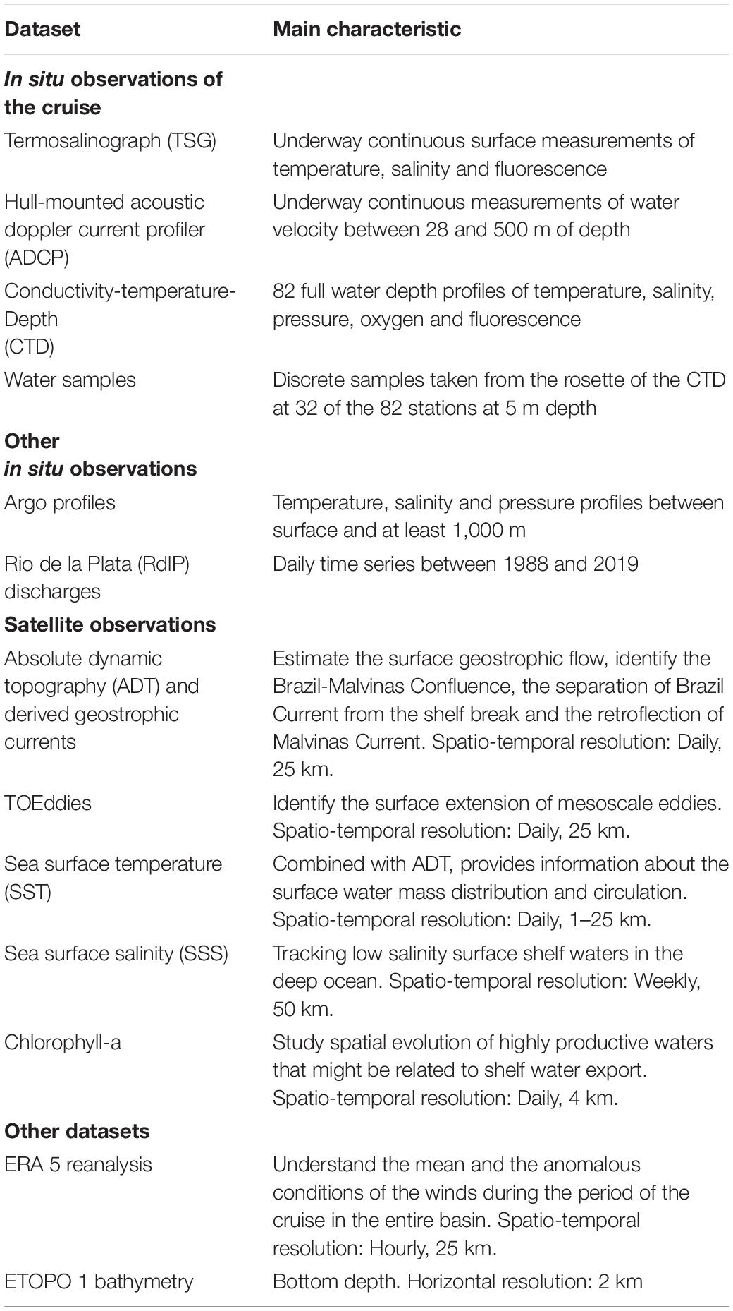
Table 1. Datasets and main characteristics related to this study.

Materials and Methods

CTD profiles were generated in 1 dbar bin average. All the gridded fields were linearly interpolated and previously smoothed with a 5 dbar centered moving average to remove spiciness from the plots. ADCP data was processed with Cascade V7.2 (Le Bot et al., 2011) with tide correction and a 16 m vertical resolution. Along and across slope velocities were computed by assuming a 40° inclination of the slope with respect to the zonal axis. Conservative temperature (Θ, °C) and absolute salinity (S_A, g kg^–1) were calculated from observations from the Thermodynamic Equation of SeaWater 2010 (McDougall and Barker, 2011) and used for the water mass characterization. Water masses in the deep ocean were classified based on neutral density (γn) ranges and thermohaline properties following Valla et al. (2018). Mixing of SACW and TW with shelf waters leads to substantial freshening over a wide neutral density range and are labeled as “others.” On the shelf (stations shallower than 200 m depth) thermohaline properties were used to identify shelf water masses following Berden et al. (2020; specified in Table 2). The data were sorted as shelf (0–200 m) and the slope (500–2,500 m) based on interpolated ETOPO1 bathymetry (Amante and Eakins, 2009), and retaining only the values within the desired ranges. In the case of Argo floats, we also filtered duplicated profiles and retained only those with good quality (flagged as 1 or 2), and the co-localized values between 1,000 and 2,500 m. To study the vertical distribution of the shelf waters with Argo floats, we interpolated the irregular sampling to a regular 10 m interval, which is the coarser resolution of the Argo profiles, in order to get the same number of observations per profile. For all the observations, we colocalized each measurement to obtain the closest satellite measurement in space and time to compare.

TABLE 2

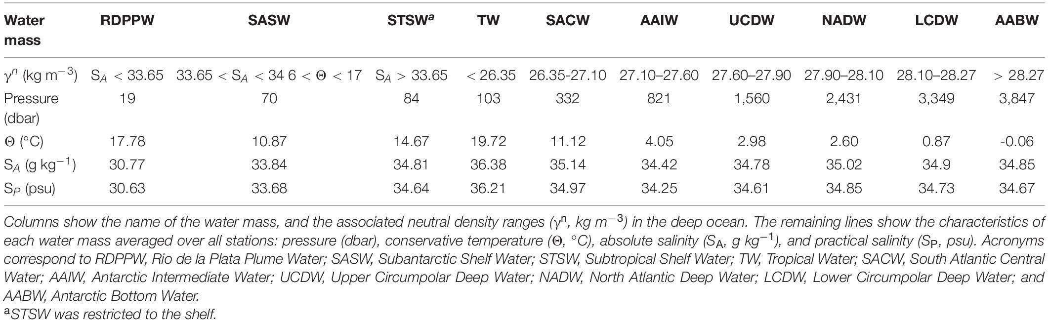
Table 2. Water masses mean characteristics in the Uruguayan Economic Exclusive Zone.

Using satellite altimetry, we followed the criteria proposed by Lumpkin and Garzoli (2011) to detect the location of the confluence over the slope “as the latitude where the surface current vectors interpolated to the 1,000 m isobath change direction from southward (Brazil Current) to northward (Malvinas Current) in 77 day low−passed velocity fields.” However, we modified it as follows. Instead of interpolating the meridional velocity to a unique latitudinal point over the 1,000 m isobath, we localized the change in the meridional currents averaged between the 500 and 2,500 m isobaths over the slope. Though no substantial differences are found in the results, our indicator is less sensitive to slight zonal displacements of the currents.

Following earlier work (e.g., Barré et al., 2011; Ferrari et al., 2017) we used three specific ADT contours as (i) a proxy for the position of the BMC (ADT 0.25 m; correlated with R² = 0.94; p < 0.001), (ii) the retroflection of MC (ADT 0 m), and (iii) the separation of BC from the shelf-break (ADT 0.5 m). Note that ADT is not a useful tool to study long-term variations because both, steric height and shift in the currents have induced variations (e.g., Fang and Zhang, 2015; Ruiz-Etcheverry and Saraceno, 2020), but it can be a useful tool to identify fronts in the past decade.

Results

Results are divided into four subsections. First, we describe the interannual contextualization of the period of the cruise and show that 2016 was a period of strong anomalous circulation conditions. Secondly, we analyze the oceanic variability during the period of the cruise. Then, we present a general description of the in situ observations, followed by the characterization of the shelf water export to the adjacent deep ocean and its relationship with the position of the BMC and mesoscale activity. Finally, based on extended Argo profiles and satellite observations, we explore the frequency of the shelf water distribution over the slope and the utility of altimetry to identify the shelf water export events.

Interannual Contextualization of the Period of the Cruise

To put the observations collected during the 2016 cruise into a long-term context we calculated the BMC index (BMCi) for the period 1993–2020. The BMCi is an indicator of the meridional fluctuations of the confluence. The seasonal amplitude of the BMCi is about 1° latitude (Lumpkin and Garzoli, 2011), reaching the southernmost and northernmost locations at the end of the summer and winter, respectively. A striking feature found in the BMCi is the trend of about 1° during the study period, or about 0.3° decade^–1. This trend represents a meridional shift from a mean position at about 38–39°S. This trend has been reported earlier both for the BMC and the separation of the BC from the shelf-break (e.g., Goni et al., 2011; Ruiz-Etcheverry and Saraceno, 2020; Bodnariuk et al., 2021) and is less than half of the trend reported by Lumpkin and Garzoli (2011) during the period 1992–2007. The reduction in linear trend when considering the past decade appears to be associated with larger amplitude meridional fluctuations observed after 2010 compared with the preceding decade (Figure 2A).

FIGURE 2

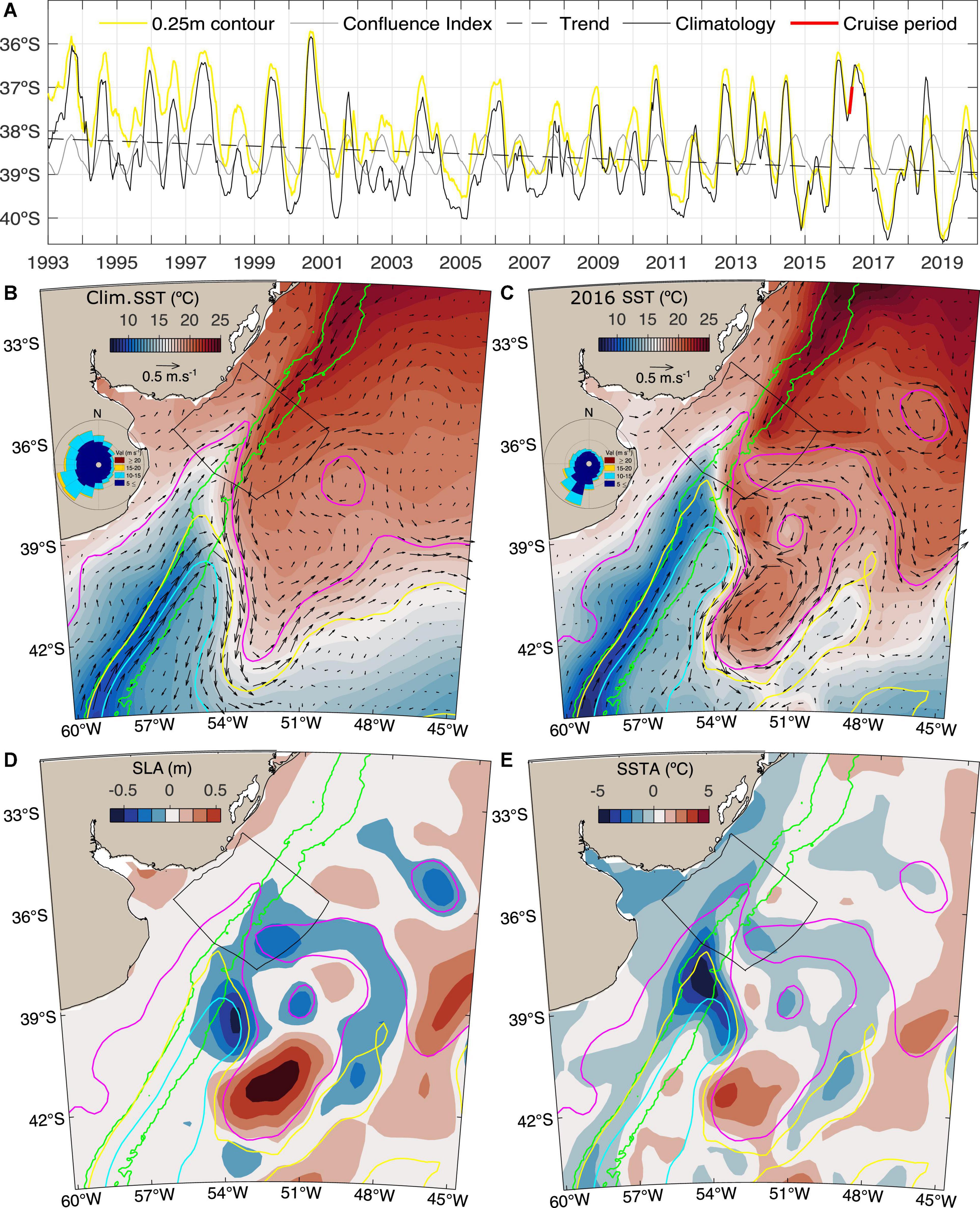
Figure 2. (A) Time series of the Brazil-Malvinas Confluence mean latitudinal position over the slope (black line). The position during the cruise is shown in red. Gray and dotted lines show the seasonal cycle and long-term linear trend, respectively. The yellow line shows the 0.25 m contour of ADT over the slope. (B) Climatological SST (°C, background color) and surface geostrophic currents (m s^–1, vectors) for April-May. All panels show the mean surface geostrophic currents displayed as black vectors, the green lines show the 500 and 2,500 m isobaths. Also shown are the 0 m (cyan), 0.25 m (yellow), and 0.5 m (magenta) ADT contours, which indicate the MC retroflection, the mean confluence position over the slope and the separation of the BC from the shelf-break, respectively. The windrose for the same period and taking all grid points is also plotted over land. (C) Same as b, but for April-May 2016. (D) Sea level anomalies (SLA, m) for April-May 2016. (E) Sea surface temperature anomalies (SSTA, °C) for April-May 2016.

During 2016, the BMC was in an anomalous northern position that lasted from the beginning of January until September, being in a record northern position relative to the climatology during the majority of the summer and at the end of autumn (Figure 2A). During the cruise, the BMC was located on average at the 82^th percentile of its latitude distribution (increasing toward lower latitude), 92^th after removing the seasonal cycle. The anomalous northward position of the BMC coincided with intense SST and ADT anomalies of about 5°C and 0.5 m when comparing inshore and offshore positions at the 2,500 m isobath (Figures 2B,C). It is also remarkable that the negative anomalies of SST and ADT, associated with the recirculation of the MC, with negative SST and ADT anomalies from 40°S 52°W up to the Uruguayan slope at 37°S 54°W (Figures 2C–E). In the entire Southwestern Atlantic basin, ERA5 data shows persistent anomalous southwesterly winds during April and May 2016, particularly during May (Wind roses in Figures 2B,C).

Likewise, mean RdlP discharges were above 95^th percentile during the first half of 2016, probably related to extreme discharges associated with the ENSO “Godzilla” event that peaked during the previous summer (Schiermeier, 2015). In particular, the previous 30-day running-mean discharge, a gross estimation of the available RDPPW over the shelf, was 56,670 m³ s^–1, more than twice the climatological mean of 25,000 m³ s^–1, corresponding to the 98th percentile in a 32-year daily time series from Borús (2017; Supplementary Figure 2).

Variability Within the Period of the Cruise and Shelf Water Export

The period of the cruise was characterized by changing atmospheric and oceanic synoptic conditions. Intensification of a low-pressure system in the South Atlantic generated strong winds (up to 23.5 m s^–1 on 25 April) and forced the vessel to return to the port of Montevideo between 26 and 29 April. The persistent southwesterly winds induced a drop in the air temperature and a large oceanic heat loss (not shown). Moreover, there was advection of cold waters under intense northeastward currents on the shelf that persisted until the end of the cruise and even longer (Proença et al., 2017). Thus, unplanned, this resulted in an 18-day sampling of the deep ocean stations (from 9 to 26 April) and a 12-day sampling of the shelf and slope stations (from 29 April to 10 May) separated by a 2 day stop in between. Henceforth we dubbed these spatio-temporal grouping of stations as the first “half” and second “half” of the cruise, respectively.

Each half of the cruise can also be split into two parts based on the mesoscale dynamical state of the ocean, lasting about a week each. During the first 10 days of the cruise, the open-ocean area south of 36°S was mostly occupied by a large anticyclonic eddy (A1) that detached from BC and moved southward (Figure 3A). Subsurface salinities up to 37 g kg^–1 were measured within A1 and the BC, and the most intense currents were observed at the periphery of A1, with speeds larger than 1 m s^–1 and reaching depths as deep as 300 dbar. As a consequence of the eddy shedding, the BC retroflection was located north of 36°S. During the following 8 days, a cyclonic eddy (C1) entered the region from the east and occupied part of the area where A1 was located the previous week, with the retroflection of the BC displacing slightly southward (Figure 3B; see also Supplementary Video 1). The second half of the cruise was characterized by the southward displacement of C1 out of the study area followed by a southward extension of BC reaching 37°S (Figure 3C). This period can also be divided into two different mesoscale dynamical regimes: from 29 April to 3 May C1 persisted as a coherent structure (Figure 3C), whereas, from 4 to 9 May, C1 displaced toward the MC (Figure 3D).

FIGURE 3

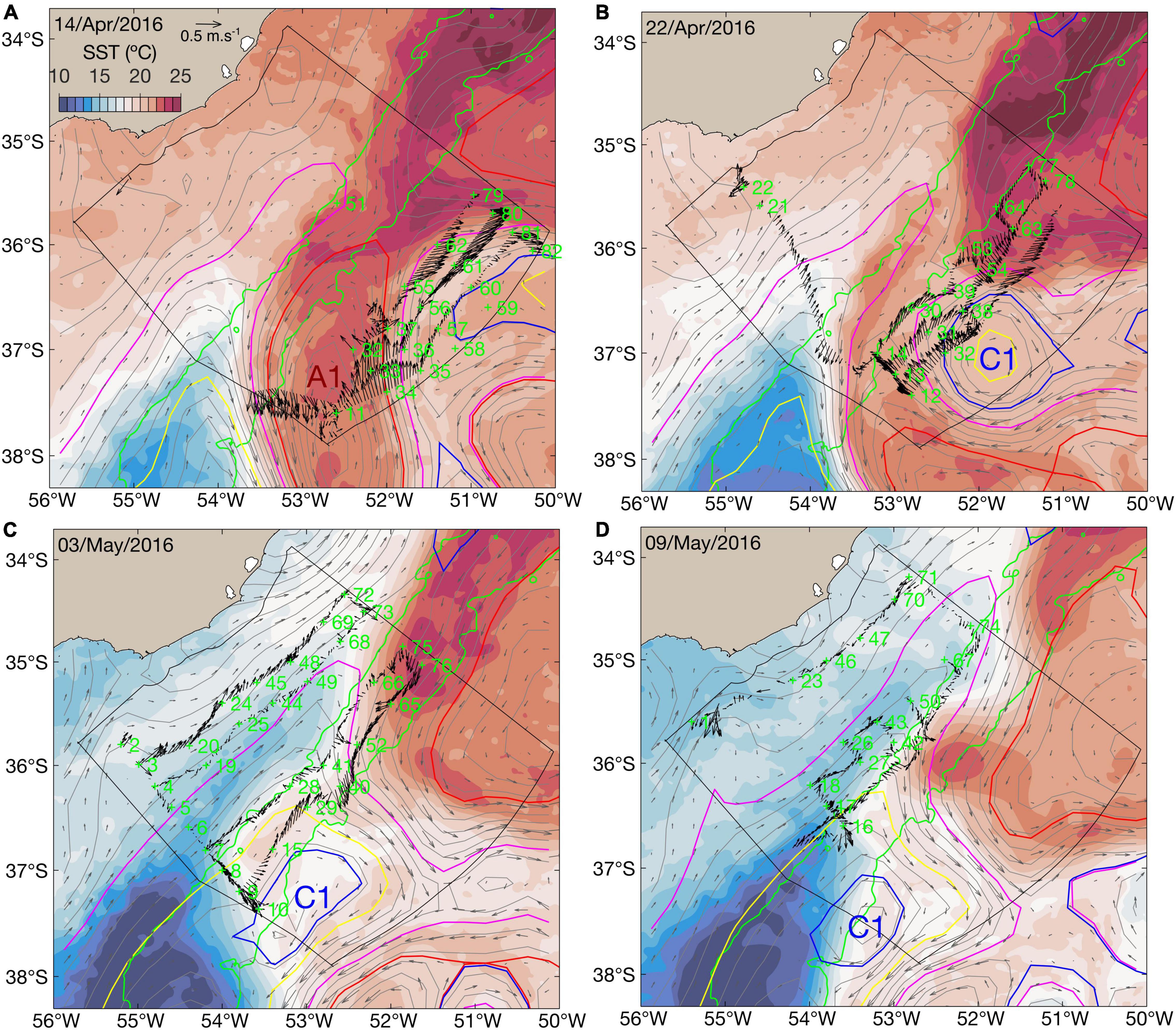
Figure 3. Representative snapshots of the oceanic synoptic situations during the cruise for (A) 14 April 2016, (B) 22 April 2016, (C) 3 May 2016, (D) 9 May 2016. Background colors represent SST (°C), while gray contours and vectors represent ADT and associated geostrophic currents, respectively. Black vectors represent the ADCP measurements averaged over the upper 100 m, which represents better the upper geostrophic circulation than the shallowest measurement, and green numbers indicate the CTD stations occupied during approximately that week. The green lines show the 500 and 2,500 m isobaths, and the 0 m (cyan), 0.25 m (yellow), and 0.5 m (magenta) ADT contours which indicate the retroflection of the main core of the Malvinas Current, the mean confluence position and the separation of the BC from the shelf-break, respectively.

In situ Observations in the Uruguayan Economic Exclusive Zone During April–May 2016

Underway surface temperature and salinity were both extremely variable in space and time during the cruise. Extreme temperature values were associated with variability from WBCs over the slope, with coldest waters (10°C) south of the Uruguayan EEZ related to the MC, and warmest waters (25°C) associated with the mesoscale activity of the BC (Figure 4B). The SST over the shelf cooled about 6°C between the beginning and the end of the cruise (Figures 4A,D). The air temperature was lower than SST during most of the cruise, up to 8°C cooler than the SST over the BC and 5°C in some parts of the shelf (Figure 4B). Surface salinity varied from 0.5 g kg^–1 close to the RdlP and 37.0 g kg^–1 in the deep ocean, with also large variations through time. The position at [35.3°S, 55°W] near station 1 close to the RdlP mouth was crossed three times 9 and 26 April, and 10 May, and the TSG salinity and temperature observations were 26.1, 26.7, and 8.5 g kg^–1, and 21.0, 18.9, and 14.6°C, respectively (Figure 4A). Due to the extreme discharges of the RdlP, MODIS Aqua image during 9 May shows the muddy RdlP water more than 100 km away from its climatological position off Montevideo (not shown; Maciel et al., 2021). This was also reflected in the anomalous low salinity water (S_A < 2 g kg^–1) observed at station 1 conducted on 9 May inshore of the RdlP turbidity front. At this station, turbidity concentration was at least one order of magnitude higher than at other stations (Figure 4C). Nitrate and phosphate were maximum also at this station, 23.42 and 2.77 μmol kg^–11, respectively. Overall, nutrients were high over the shelf and in the cold waters over the southern portion of the slope, with maximum values close to the RdlP and in the southern shelf break covered by MC, and low over the deep ocean stations (Figure 4F).

FIGURE 4

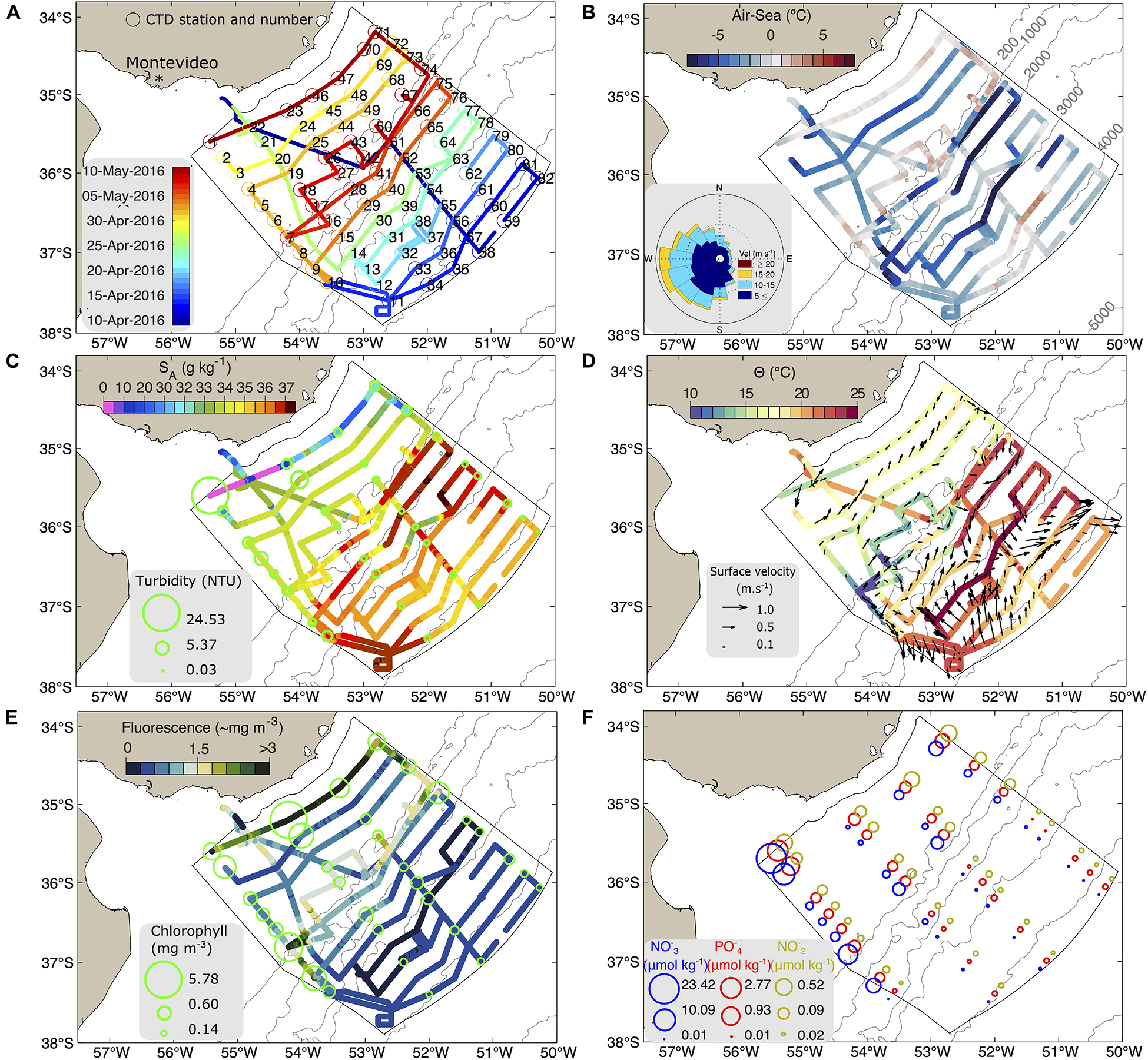
Figure 4. Near-surface observations during April-May 2016. (A) Cruise track and station numbers. (B) Difference between air and sea surface temperature (°C). Wind rose from ship measurements (m s^–1) during the cruise period is also shown. (C) Absolute Salinity (S_A, g kg^–1). The size of the green circle represents specific turbidity measurements (NTU). (D) Sea surface temperature (°C) and currents (m s^–1) from the ADCP averaged over the upper 100 m (black vectors). (E) Chlorophyll-a from fluorescence. The symbol size represents the in situ chlorophyll-a measurements (mg m^–3). (F) Nitrates (NO^–₃, μmol kg^–1, blue symbols), Phosphates (PO^–₄, μmol kg^–1, red symbols), and Nitrites (NO^–₂, μmol kg^–1, green symbols) concentration at 5 m depth.

Surface chlorophyll-a was mostly positively correlated with the nutrient distribution, decreasing toward the deep ocean. Maximum values were measured near the coast immediately offshore from the turbidity front (10 < S_A < 25 g kg^–1), although they did not peak at station 1 in the RdlP waters, where nutrient values were maximum, due to the effect on light attenuation in muddy waters (e.g., Carreto et al., 2003; Kruk et al., 2015; Martínez and Ortega, 2015). High surface fluorescence and chlorophyll-a were also observed in the southernmost area of the Uruguayan EEZ, at stations 7 and 9 over the outer shelf and slope, over the Ewing Terrace and Rio de la Plata canyon under the influence of the MC retroflection at about 37°S 54°W. These stations showed the coldest surface waters and high concentration of nutrients (Figures 4D–F), and also the highest integrated fluorescence in the CTD profile (3.15 mg m^–3) in the upper 50 m (Figure 4D), as these stations were occupied at the end of a chlorophyll bloom that took place 10–25 April according to satellite observations (Supplementary Video 1). The intense front observed in this region, and the mixing with shelf waters probably triggered this bloom. In contrast, a band of high nutrient low chlorophyll was formed in the outer shelf from 26 April until the end of the cruise, probably due to the fully mixed water column by strong southwesterly winds (wind rose from ship measurements in Figure 4B) and intense northeastward currents.

In agreement with satellite geostrophic observations, observed upper-ocean currents (averaged over the upper 100 m) displayed two clearly different regimes in the shelf and deep ocean (Figures 1, 4D). Despite the stations over the shelf being occupied over a period of nearly 1 month, northeastward surface velocities prevailed in this region, while velocities over the deep ocean were higher and with different directions due to mesoscale eddies and the retroflection of the major currents. The BC appeared as a southward flow in the northern half of the Uruguayan EEZ over the 2,000 m isobath with Θ > 23°C and S_A > 36 g kg^–1, respectively, and very low chlorophyll-a and nutrient concentration. A retroflection of the BC, usually referred to as “overshoot,” was observed at about [36.5°S, 52°W] between the 3,000 and 4,000 m isobaths (Figure 4D).

Below the surface, the full-depth CTD profiles showed three different water masses on the shelf and seven water masses in the deep ocean (see Table 2 for acronyms and mean properties). From the coast to the 50 m isobath (about 80–100 km), the study area was mostly filled with RDPPW. With S_A < 33.65 g kg^–1, it is the most nutrient-rich and high-chlorophyll-a water mass. SASW prevailed toward the outer shelf, narrowing considerably toward the north as the shelf also narrows as it tends to be replaced by STSW. A very small fraction of the shelf was occupied with STSW which was mainly found in the outermost stations in the northern part of the shelf (Figure 5A). The observed transition between SASW and STSW agrees with the location of the Subtropical Shelf Front determined from historical data (Piola et al., 2000).

FIGURE 5

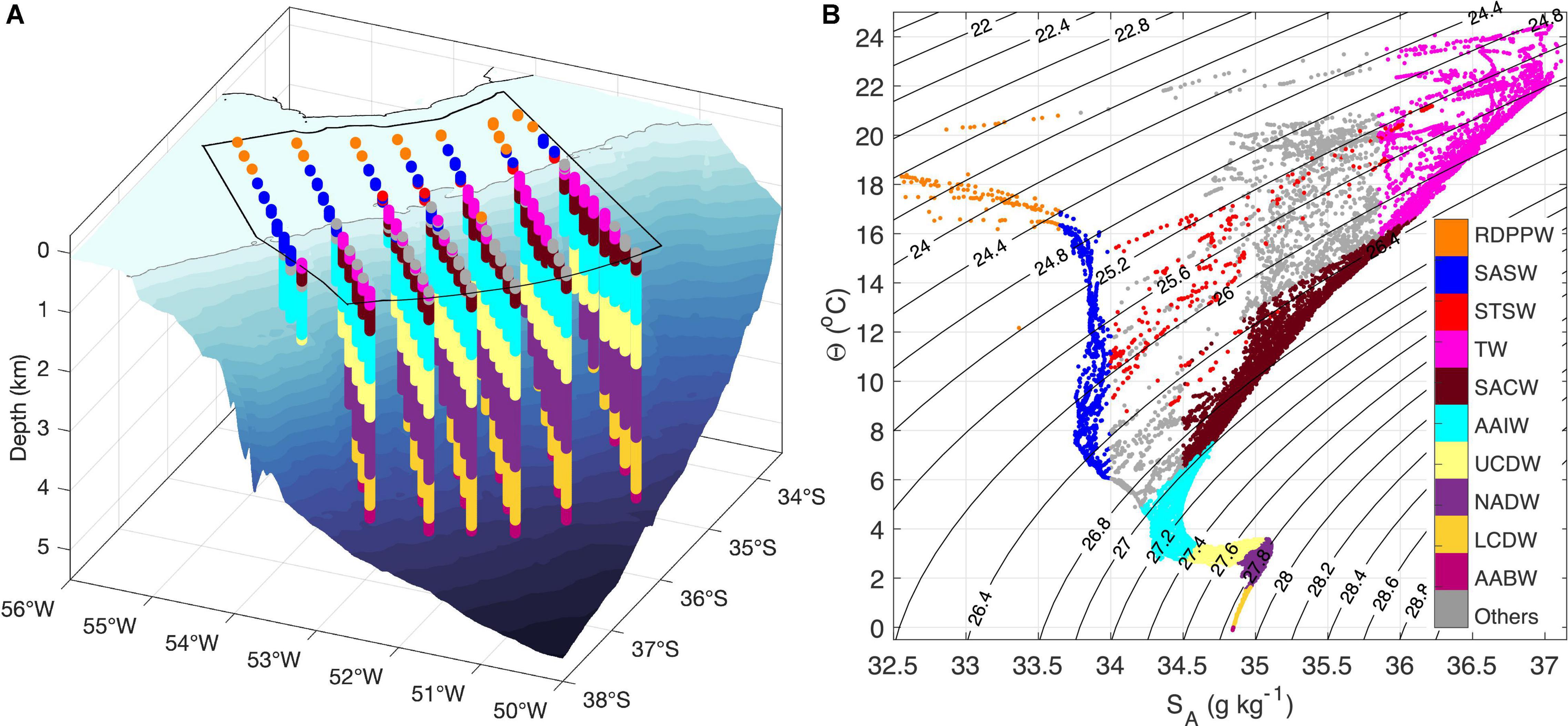
Figure 5. (A) 3-D visualization of the CTD profiles occupied during the cruise. Each vertical line represents a CTD profile and the colors within each line a specific water mass as shown in (B). The black polygon at the surface shows the Uruguayan EEZ and the gray line shows the 200 m isobath. (B) Θ-S_A diagram of the CTD profiles shown in (A) and water masses whose hydrographic characteristics are described in Table 2.

The deep ocean exhibited TW and SACW in the upper layers. The data display evidence of intrusions of SASW and STSW at several vertical levels within the relatively warm and salty TW and SACW. Large amplitude thermohaline intrusions observed in this region are ubiquitous of the confluence region (e.g., Piola and Georgi, 1982; Bianchi et al., 1993; Orúe-Echevarría et al., 2021), and are indicative of intense isopycnal mixing between the adjacent water masses with contrasting thermohaline properties (Figure 5B). Water masses found at deeper depths were those characteristics of the region: UCDW, NADW, LCDW, and AABW, respectively (Maamaatuaiahutapu et al., 1992, 1994; Provost et al., 1995; Valla et al., 2018; Table 2 and Figure 5B).

Surface Water Export

In this subsection we describe the evidence suggesting the export of shelf waters to the adjacent open ocean and discuss the processes involved. A well-known process exporting surface shelf water consists of brackish RDPPW and mixtures of shelf waters being advected offshore by the mesoscale activity of the BC. These have been detected by satellite SSS observations (Guerrero et al., 2014) and in numerical simulations (Matano et al., 2014). Export of low-salinity shelf waters is also apparent in hydrographic observations from the BC and near the confluence (Gordon, 1989; Provost et al., 1996; Piola et al., 2008; Berden et al., 2020). The high-resolution UEEZ observations reported here provide valuable information from the region of detachment of shelf waters. We identified an export event during the first half of the cruise, although only the initial part of the low salinity plume detaching from the shelf was detected in satellite SSS (Supplementary Figure 3C), suggesting that the coarse satellite observations cannot properly resolve it. Nevertheless, satellite chlorophyll-a provides useful information about the spatial structure of the export due to the contrasting values between shelf and the open ocean waters (such as during 24 April at 36°S 52.5°W, Figure 6). The high chlorophyll-a filament consisted of a brackish water filament detached from the shelf along the BC retroflection (Figure 6A). The TSG measurements across the filament and 2 CTD profiles occupied that day display the 3-D structure of the low salinity RDPPW filament. The filament was 70 km wide and 20 m deep according to the TSG and the CTD profiles inside the filament, respectively (Figures 6B,C). Within the 70 km wide filament and the ADCP measurements in the upper 60 m, which better represent the filament, the mean across-slope velocity was 0.30 m s^–1 (Figures 6B,C), and the off-shore estimated transport 0.42 Sv.

FIGURE 6

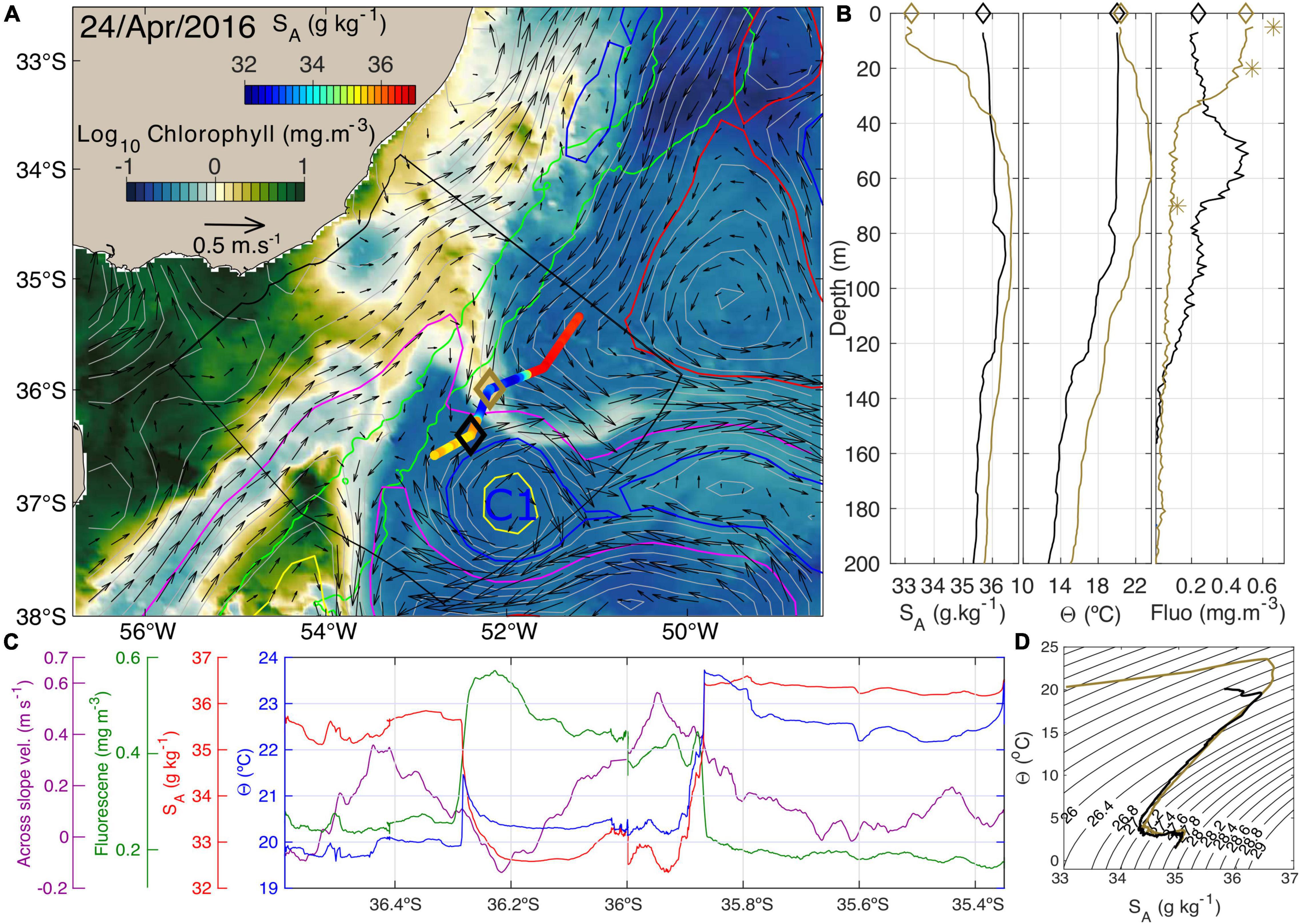
Figure 6. (A) Satellite chlorophyll-a and surface geostrophic currents on 24 April 2016. Gray lines show ADT contours. Underway near-surface salinity measurements are indicated along the cruise track across the filament, color-coded by SSS (color scale above). Black and brown diamonds indicate the location of the CTD profiles 39 and 53 collected that day. The green lines show the 500 and 2,500 m isobaths. Yellow and magenta colors represent the 0.25, and 0.5 m ADT contours, respectively. Red and blue contours refer to anticyclonic and cyclonic eddies, respectively. (B) Upper 200 m profiles of Absolute Salinity (S_A, g kg^–1), Conservative temperature (Θ, °C), and fluorescence (mg m^–3) from the CTDs 39 and 53. Brown and black lines correspond to stations 53 and 39 carried out within and outside the low-salinity filament, respectively. Asterisks show the laboratory chlorophyll-a measurement from the water samples collected at station 53. (C) Underway TSG measurements on the transect occupied across the low-salinity filament shown in (A). The panel shows: Upper 60 m across-shore velocities from the ADCP (magenta, m s^–1, and absolute salinity (red, S_A, g kg^–1), conservative temperature (blue, Θ,°C), and fluorescence (green, mg m^–3). (D) Θ^–S_A diagram of stations 53 and 39 in brown and black, respectively.

The northern edge of the filament showed very sharp gradients. In 20 km, S_A decreased from 36.45 to 32.34 g kg^–1, temperature from 23.75 to 20.1°C, and fluorescence increased from 0.2 to 0.4 mg m^–3. Also, very close to the front, a local maximum of 0.7 m s^–1 in the across-slope velocity was observed (Figure 6C). The southern side of the filament showed a less intense fluorescence gradient, probably because the region north of the filament was occupied by oligotrophic BC water, while cold-core (< 19.5°C), high-fluorescence (> 0.35 mg m^–3) eddy C1 was located south of the filament. The CTD profile occupied within the filament showed that the brackish water extended downward to about 20 m depth, characterized by RDPPW properties (S_A < 33.65 g kg^–1; Figure 6D) and high fluorescence (> 0.45 mg m^–3). It is remarkable also that the vertically integrated fluorescence in the upper 140 m was higher in the CTD profile outside the filament, but the peak was below 40 m of depth and it was not apparent in satellite observations (Figure 6B).

Subsurface Water Export

The in situ data also showed evidence of subsurface shelf-water export over the slope located at the BMC during the second half of the cruise. The gridded absolute salinity field from CTD profiles averaged between 40 and 120 m depth shows a low salinity tongue of SASW (S_A < 34 g kg^–1; < 12°C) being exported offshore up to the outer slope, approximately over the 2,000 m isobath (Figure 7A). Most of the CTD profiles over the slope were occupied within the first week of May 2016. Hence, the altimetry map of 3 May might be taken as representative of the regional circulation during that week (Figure 7B). The SASW tongue was located between the BMC and the BC separation from the shelf (yellow and magenta contours in Figure 7B, respectively), with geostrophic velocities oriented perpendicular to the slope toward the open ocean. The Θ-S_A diagram of that section shows a clear transition from subantarctic waters within the MC to subtropical waters from the BC (Figure 7C). Three CTD profiles showed the presence of SASW. The freshest SASW variety was observed at the BMC (station 40 at 36.2°S 52.6°W), with a homogeneous layer of 33.76 g kg^–1 found between 70 and 130 m of depth (Figures 7C,F). The next CTD profile to the south showed evidence of SASW located between 160 and 230 m of depth. Here, SASW properties showed evidence of mixing with saltier waters with a relative maximum of 34.45 g kg^–1 at 200 m of depth. Finally, the third profile with SASW was located in the southernmost CTD profile (station 9), which displayed a Θ-S_A structure typical from the MC over the slope (Figures 7B,C).

FIGURE 7

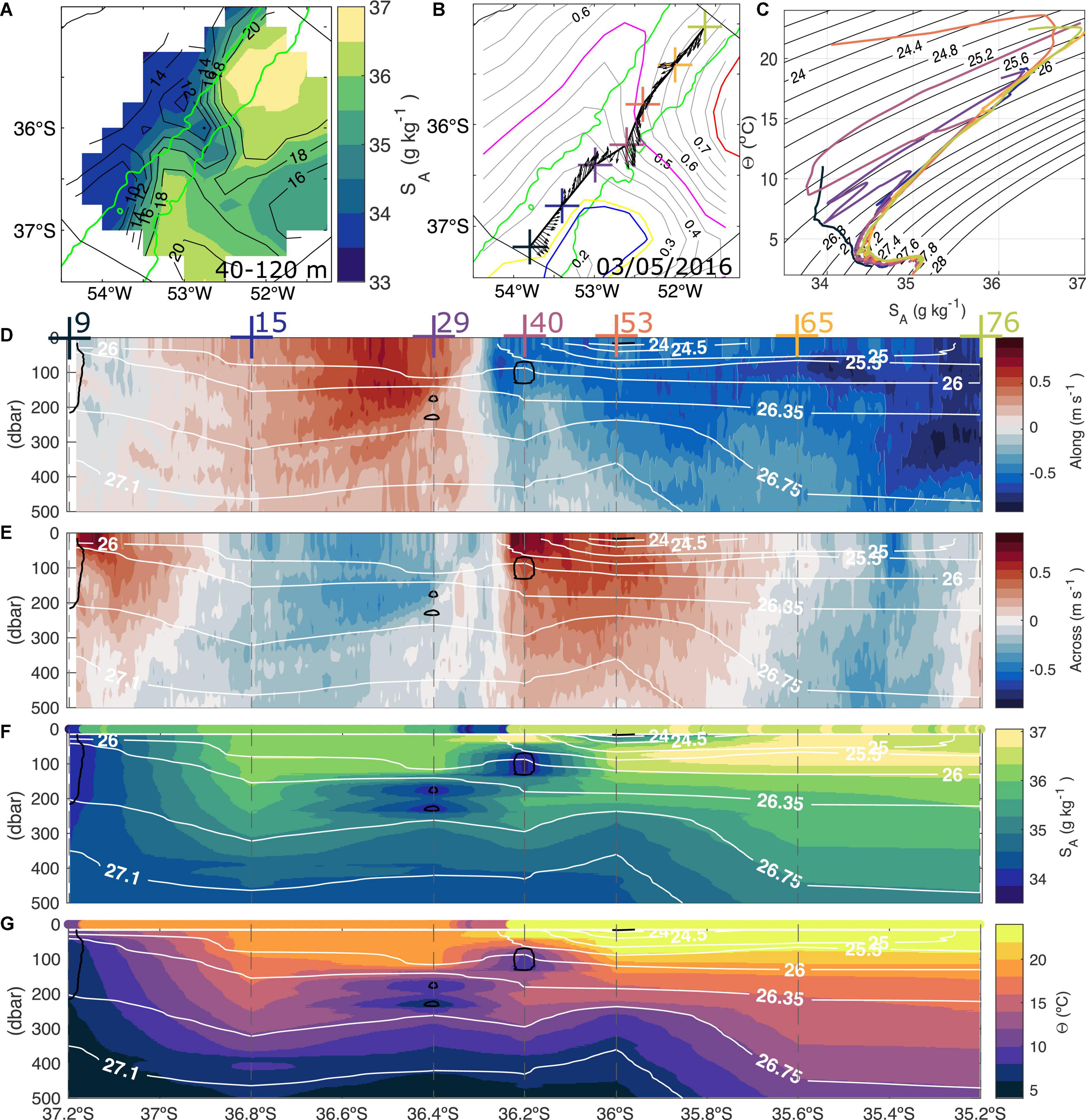
Figure 7. Overview of the export of Subantarctic Shelf Waters at the Brazil-Malvinas Confluence during the first week of May 2016. (A) Mean absolute salinity (shades) and conservative temperature (contours) averaged over the 40–120 m depth interval. (B) Location of CTD stations occupied over the main BC and MC on 2 and 3 May 2016 approximately over the 1,600 m isobath. Vectors show the upper 100 m velocity field from the ADCP, and gray contours the ADT, with the yellow and magenta lines representing the BMC and the separation of BC from the shelf break, respectively, and blue and red contours the cyclonic and anticyclonic eddies, respectively. Colored crosses indicate the profiles in the Θ-S_A diagram in (C). The panels below show: (D) Along slope velocity (m s^–1). (E) Across slope velocity (m s^–1). (F) Absolute salinity (g kg^–1), and (G) Conservative Temperature (°C), respectively. TSG underway measurements are also plotted above panels (F,G). Black contours enclose shelf water (S_A < 34 g kg^–1), gray lines are contours of constant neutral density, and dotted lines the CTD profiles location in all panels.

We next constructed an along-slope section over the main core of the WBCs, occupied during the period 3–5 May, when eddy C1 was merging with the MC. We did so from continuous ADCP velocity measurements and seven CTD profiles occupied along the 285 km section (stations 9, 15, 29, 40, 53, 65, and 76 from south to north, respectively; Figures 7D–G). The CTD profile containing the homogeneous layer of SASW at the BMC (station 40) was separated from the two closest stations by about 40 km. Therefore, we assumed that the horizontal extension of this layer was 40 km, half the distance between the two closest stations and approximately the extension of the low salinity surface signature from the TSG, with an uncertainty of 40 km. The mean across-slope velocity measured from the ADCP within the representative 40 km of the CTD station and the 70–130 m depth containing the homogenous SASW layer was 0.38 m s^–1. Hence, our estimate of the offshore export of SASW at the BMC is 0.91 ± 0.91 Sv.

An across-slope CTD transect allowed us to identify and track the core of the SASW from the shelf to the deep adjacent ocean, although it must be interpreted with caution because the transect is a collection of non-synoptic data. The profiles showing the layer of SASW immediately outside the shelf were conducted on 4 and 6 May 2016. The reconstructed transect shows a 60 m thick layer of SASW (Θ between 6–12°C and S_A 33.75–34 g kg^–1) flowing below the γ = 25.7 kg m^–3 isopycnal. This vein of SASW left the surface at the shelf break where it subducted, reaching 130 m of depth at the 2,300 m isobath (Figure 8A). The exported SASW might have reached deeper levels, but this cannot be assessed with the cruise data as the following offshore CTD profiles along this transect were collected 10 days earlier (Figures 8A,B).

FIGURE 8

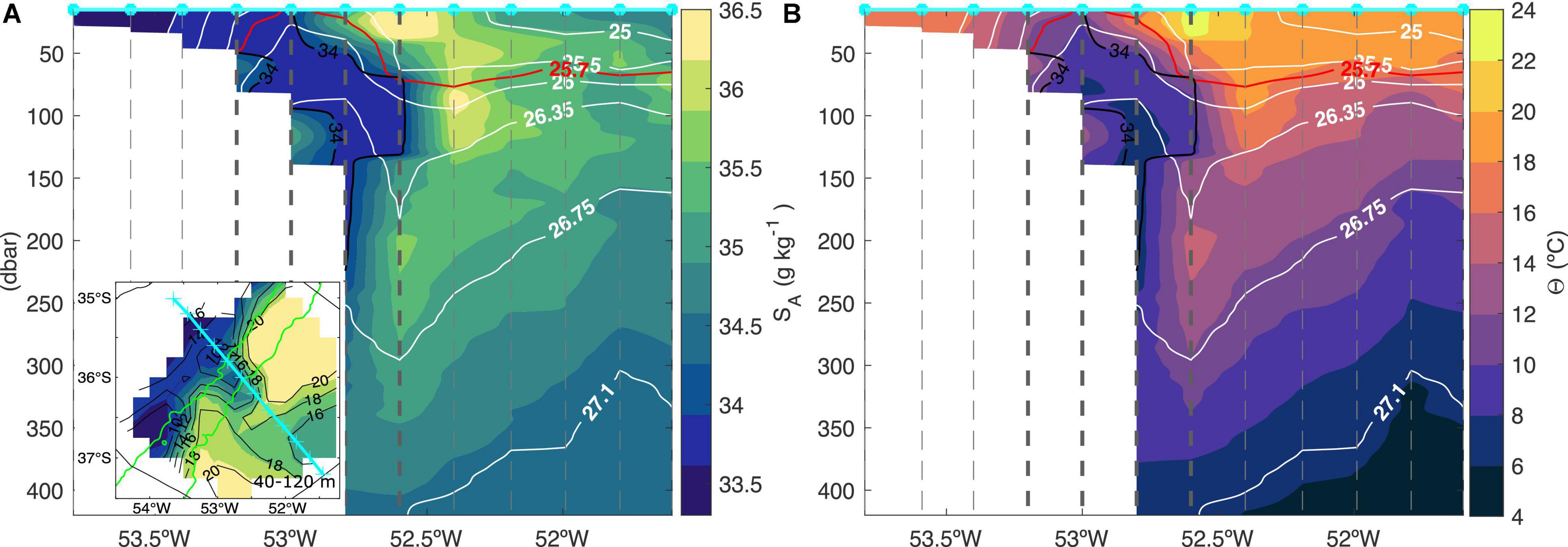
Figure 8. Across-slope section. (A) Absolute salinity (S_A, g kg^–1). The inset shows the S_A field averaged over the 40–120 m depth interval, and the cyan line shows the transect. (B) Conservative temperature (Θ,°C). The 34 g kg^–1 contour delimiting Subantarctic Shelf Waters is drawn in black. Neutral density contours are shown in gray, with the 25.7 kg m^–3 shown in red. Dotted lines show the location of the CTD profiles used to make the section, and the bold dotted lines correspond to those stations considered as synoptic conducted between the 4 and 8 May.

In this case, no low salinity signature was identified in satellite SSS (Supplementary Figure 3D). Chlorophyll-a showed a relative maximum at the same location where the SASW offshore export is apparent in the observations. However, the signal was very weak and might have also been locally generated instead of being advected (Supplementary Video 1). On the other hand, geostrophic currents derived from satellite altimetry show a high correlation and the lowest root mean square error (RMSE) with ADCP measurements at a depth of 110 m (p < 0.01; R² 0.82 and 0.35; RMSE 0.25 and 0.23 m s^–1, for along and across slope velocities, respectively; Supplementary Figure 4). Therefore, although satellite observations cannot directly detect the subsurface export of SASW, satellite altimetry might be used as an indicator of where and when such export events take place.

Shelf Waters Detection From Argo Floats and Satellite Observations

In this section, we explore the frequency of RDPPW and SASW over the slope and their relationship with altimetry using long-term Argo floats and satellite observations. The Hovmoller diagram constructed from satellite geostrophic currents and SSS in the zonally averaged slope shows that most of the observed across-slope positive (offshore) velocities occur between the BMC and the separation of the BC from the shelf break, following the described seasonal migration of the BMC (see black and magenta contours in Figures 9A,B). It is also remarkable that a local maximum in across-slope velocity (0.3–0.4 m s^–1) is observed when the BMC reaches its extreme highest and lowest latitude. Also, across-slope velocities higher than 0.1 m s^–1 are observed during winter north of the separation of the BC from the shelf break at about 33°S (Figure 9A).

FIGURE 9

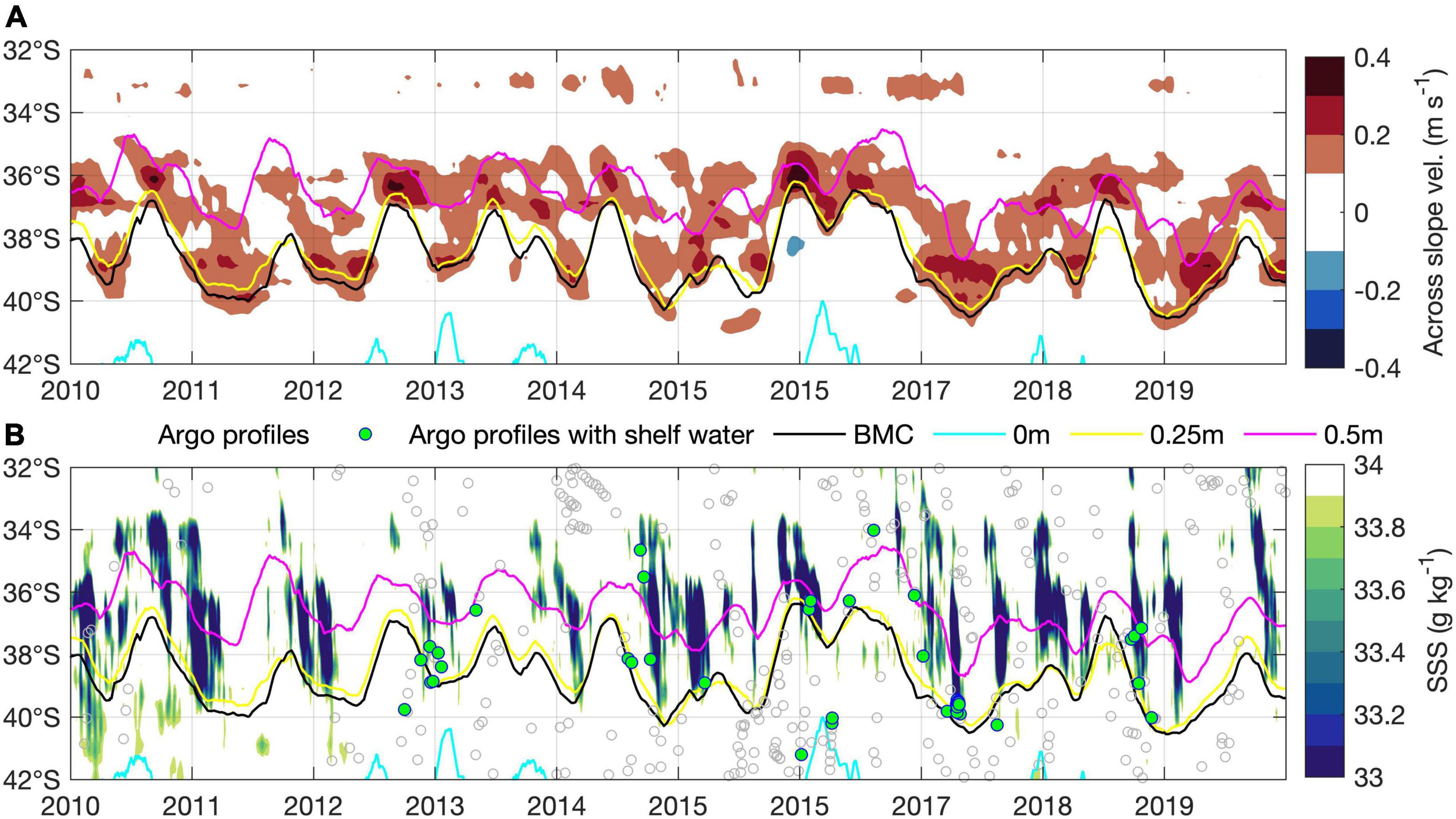
Figure 9. Hovmoller plots of latitude vs. time over the zonally averaged slope in the Southwestern Atlantic. In both panels, the black contours represent the BMC position, and the 0, 0.25, and 0.5 m contours of ADT are shown in cyan, yellow, and magenta, respectively. (A) Surface across-slope velocity (m s^–1). (B) Sea Surface Salinity (SSS, g kg^–1). Gray circles show Argo profiles located over the slope, and green circles indicate data from Argo profiles in which shelf waters were observed. Note that only the period where SSS is available is plotted.

Satellite SSS with shelf water characteristics (S_A < 34 g kg^–1) are observed over the slope north of the BMC in most of the cases. They display a clear seasonal cycle, mostly determined by the southward extension of the BMC, reaching higher latitudes at the end of the summer (Figure 9B). From the 431 Argo profiles located between the 1,000 and 2,500 m isobaths and from 32 to 42°S over the southwestern Atlantic slope, 59 (12%) contained shelf waters, while 32 (7%) contained exclusively RDPPW. Most of the profiles containing shelf waters were located north or at the BMC, in particular between the BMC and the separation of BC from the shelf-break (Yellow and magenta contours in Figure 9B, respectively). The shallowest salinity observations from the 427 Argo profiles were significantly correlated with satellite SSS (p < 0.01; R² = 0.64). Co-localized Satellite SSS measurements showed less variance than in situ observations, as expected from its coarse space-time resolution. Nevertheless, the RMSE was 0.78 g kg^–1, which might be an acceptable value to identify RDPPW, yet too large to correctly single out SASW. While shelf water (S_A < 34 g kg^–1) was detected in the shallowest measurement (1–10 m) of 54 of the 427 Argo profiles, the corresponding co-localized satellite SSS detected 58.

Argo profiles in the slope co-localized with ADT show values ranging between -0.25 and 0.96 m, with remarkable differences in the Θ-S_A signature depending on which side of the fronts the floats were localized (Figures 10A,B). Figure 10A also shows three Θ-S_A diagrams from Argo floats containing shelf waters similar to CTD stations occupied during the 2016 cruise (station 53 in Figure 6D and stations 9 and 40 in Figure 7C). The histogram in Figure 10C displays the number of Argo profiles as a function of ADT. The maximum frequencies are observed in the −0.1 to −0.05 m and 0.6–0.65 m intervals. Argo profiles containing SASW spread over a wide range of ADTs (−0.15 and 0.6 m), while the profiles containing exclusively RDPPW are restricted to the 0.25 and 0.6 m range, thus falling between the BMC and the separation of the BC from the shelf break. In particular, ADT ranges between 0.35 and 0.45 m contain the majority of Argo profiles with RDDPW, with 23 out of 38 profiles (∼60%) within these two class intervals (Figure 10C). Inspection of the vertical distribution of shelf waters in the Argo profiles, both RDPPW and SASW are most frequently observed in the upper ocean interval (10–20 dbar). However, while RDPPW is exclusively restricted to the upper 40 dbar, these data show that SASW can reach depths of 200 dbar (Figure 10D).

FIGURE 10

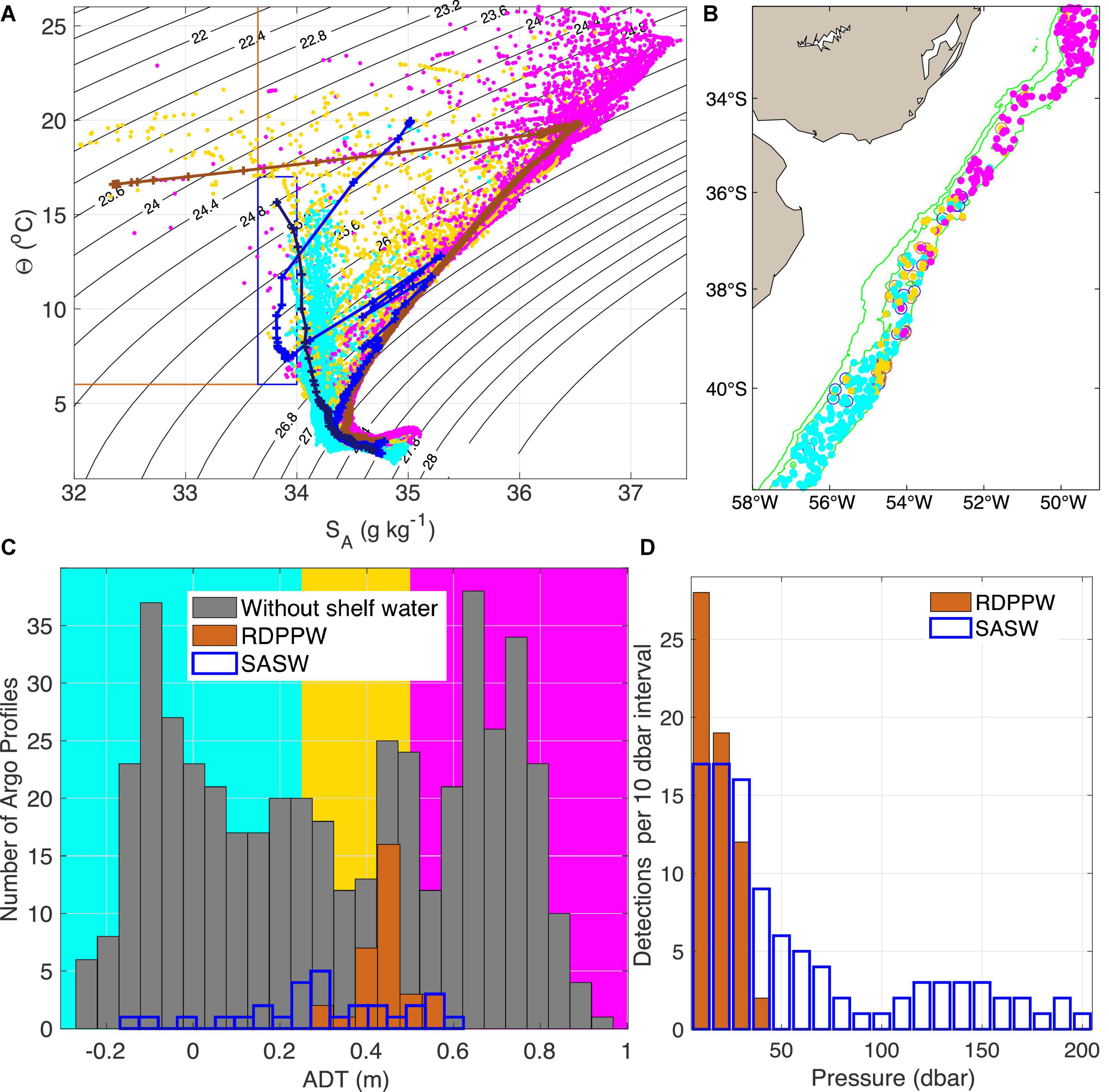
Figure 10. (A) Θ-S_A diagram of Argo profiles over the Southwestern Atlantic slope co-localized with ADT values. Colors represent ADT values < 0.25 m in sky-blue (MC), > 0.5 m in magenta (BC), and yellow in between (BMC) in panels (A,B). Blue and brown polygons represent the thermohaline intervals for Rio de la Plata Plume Water (RDPPW) and Subantarctic Shelf Water (SASW), and the three colored Θ-S_A diagrams are example profiles similar to those containing shelf water observed in the deep ocean during the 2016 cruise. (B) Argo profiles locations following the same color code as in (A). (C) Histogram of the Argo profiles co-localized with ADT over the slope. (D) Histogram of the pressure at which Rio de la Plata Plume Waters (RDPPW, brown) and Subantarctic Shelf Waters (SASW, blue) are found in Argo profiles located over the slope.

Summary and Conclusion

The hydrographic cruise that took place in April–May 2016 in the Uruguayan EEZ provided an unprecedented dataset to investigate local water masses, ocean dynamics, and cross-shelf exchanges at the Brazil Malvinas Confluence. Despite the survey covering a relatively small area, our study shows that it is characterized by a highly variable and dynamic environment. Water properties can fluctuate from below 0°C to over 25 °C in conservative temperature and from almost freshwater to over 37 g kg^–1 in absolute salinity. The region hosts intense western boundary currents and mesoscale activity developing offshore, displaying large oceanic space-time variability at all scales (from synoptic, to interannual and interdecadal) driving cross-shore exchanges.

The first half of 2016 was an anomalous period in the southwestern Atlantic in terms of atmospheric and oceanic circulation. It was characterized by intense southwesterly winds, negative SST anomalies, and large Rio de la Plata discharges. By extending the Brazil Malvinas Confluence latitudinal position index of Lumpkin and Garzoli (2011), we showed that the confluence was located anomalously north during the first half of 2016, occupying the Uruguayan EEZ when the in situ survey was conducted.

In this work, we focused on cross-shelf exchanges as they have important consequences for carbon export, water masses transformations, and marine biodiversity. Previous studies provide evidence that, regionally, shelf water export is closely related to the confluence position (e.g., Matano et al., 2014; Berden et al., 2020; Orúe-Echevarría et al., 2021; Figure 11A). This control is somehow expected since the Brazil and Malvinas currents generate a barotropic pressure gradient that extends into the shelf controlling the outer shelf circulation (Palma et al., 2008; Matano et al., 2010). Our analyses provide evidence of the 3-D structure and evolution of two different kinds of shelf water export associated with the BMC dynamics: one related to Rio de la Plata waters that remain confined to the surface layers; the other involves SASWs that subducts under the subtropical thermocline while crossing the slope. To understand the dynamical setting associated with these processes and to assess their significance in time we used a combination of different observations that include the cruise hydrographic data, Argo profiles, satellite maps of SSS, SST, ADT, and chlorophyll-a, and a recently developed eddy detection algorithm.

FIGURE 11

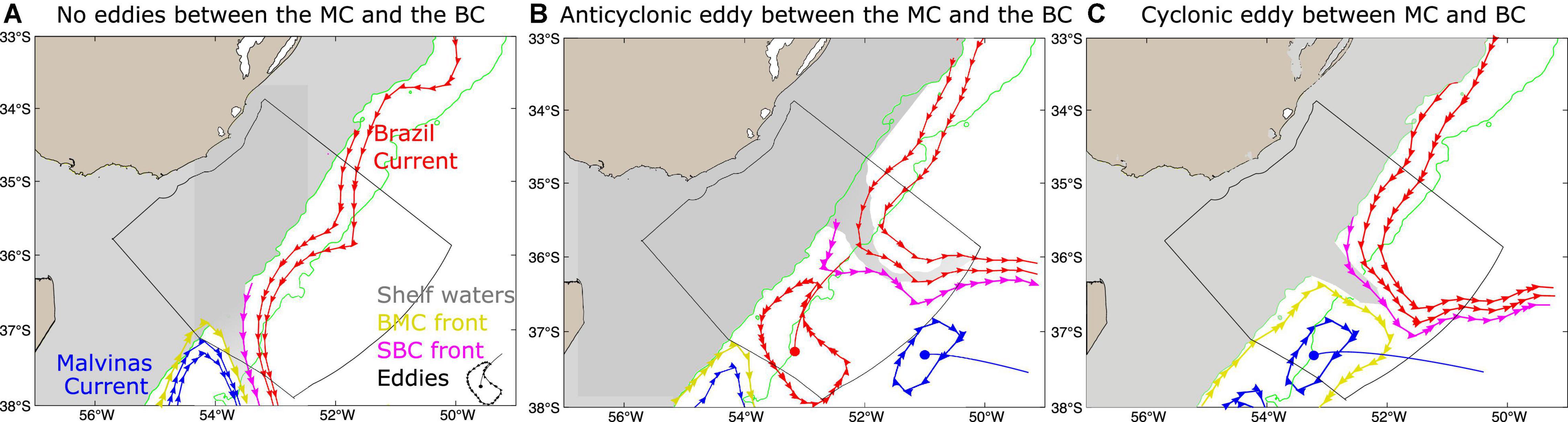
Figure 11. Schematic circulation patterns of 3 shelf water export situations in the Uruguayan EEZ. BMC stands for Brazil-Malvinas Confluence and SBC for Separation of Brazil Current from the shelf-break. Shelf waters (S_A < 34 g kg^–1) are shown in gray. Green lines show the 500 and 2,500 m isobaths. (A) Without eddies between the Brazil Current and Malvinas Current. (B) With an anticyclonic (C) cyclonic eddy between the main currents, respectively.

A near-surface export of shelf water consisted of a thin off-shelf layer of Rio de la Plata waters following the path of the retroflection of the Brazil Current after an anticyclonic eddy shedding that dissipated after 10 days due to strong winds that mixed the stratified plume (Figure 11B). In addition, the hydrographic observations reveal a subsurface export of SASW. In this case, the driving mechanism also appears to be associated with mesoscale dynamics triggered by the merging of a cyclonic eddy with the Malvinas Current at the confluence with Brazil Current (Figure 11C). This generated intense off-shelf velocities at the shelf break. Evidence of subsurface export of shelf waters based on hydrographic and lowered ADCP observations near the BMC has been recently reported by Berden et al. (2020, their Figures 4C, 8E). The novelty of this study relies on the availability of closely spaced along-slope sections which reveal the detailed structure of the cross-shelf fluxes. Combining these in situ and satellite observations we reconstruct the 3-D field, quantify the export, and associate mesoscale ocean dynamics as the driving mechanism.

Using numerical simulations, Matano et al. (2014) showed that a time-averaged convergence of volume of about 1.21 Sv in the along-shore flow of SASWs (1.15 Sv) and STSW (0.038 Sv) and the inflow of Rio de la Plata waters (0.024 Sv) between 34 and 38°S must be exported offshore. The 1.21 Sv could hardly be achieved by the exported low salinity RdlP plumes, but the sum of both surface and subsurface export as observed in this work is closer to. In addition, Franco et al. (2018) using numerical simulations showed that released neutrally buoyant particles equally distributed in the vertical at 38°S over the shelf were exported all along the shelf-break between the retroflection of the Malvinas Current and the Subtropical Shelf Front at about 32°S. Most of the neutrally buoyant particles were exported at the BMC, in particular within the 50–200 m layers. They also showed that as SASW was exported, it rapidly became saltier. The intense mixing observed over the slope together with the fact that the difference between SASWs and the surrounding ocean waters can be less than 0.2 g kg^–1, makes it difficult to detect this water mass based only on salinity differences with the surrounding waters, as the shelf water freshwater signature rapidly fades as shown by Franco et al. (2018).

By using Argo profiles located within the southwestern Atlantic slope, we provide evidence of the presence of Rio de la Plata waters and SASWs between the separation of the Brazil Current from the shelf-break and the confluence and at the same depths as observed during the 2016 cruise. At specific values of absolute dynamic topography of 0.35–0.45 m, we found shelf waters over the slope in more than half of the Argo profiles, further suggesting the export of shelf waters at this location is relatively frequent. Also, by inspecting Argo profiles together with satellite surface salinity we show that SASWs is often found over the slope, especially within the shallow branch of the Malvinas Current. Because of the similarity between SASWs and surrounding waters thermohaline properties and the intense mixing taking place over the slope, detection of shelf waters within this current is challenging. Nonetheless, by combining in situ water velocity measurements and concomitant satellite altimetry observations we found evidence of SASWs along the BMC. In contrast, Rio de la Plata waters are more easily detectable in the open ocean due to their low salinity characteristics.

We also provided evidence that, although satellite surface salinity reveals shelf water exports (Guerrero et al., 2014), the coarse resolution of satellite data limits the ability to detect the fine structure and temporal evolution of the exported waters. This suggests that several export events might not be properly captured by satellite surface salinity. Chlorophyll-a, which has higher resolution especially under clear sky conditions, could be a complementary tool to detect these freshwater export events, but need to be contrasted with other salinity observations, as high chlorophyll-a filaments could be associated with several other processes not related to shelf-waters. Combination of different observations in the future (e.g., satellite Chlorophyll-a and salinity observations) could provide more insights on detecting and characterizing shelf water export events.

Another useful approximation to study shelf water export processes are high-resolution numerical models, as they reproduce the shelf-water export, especially when the confluence and the separation of the Brazil Current from the shelf break are along the same front (Berden et al., 2020; Orúe-Echevarría et al., 2021), but probably also to better simulate the impact of mesoscale eddies, like those observed during the 2016 cruise (Figure 11). Recent numerical simulations highlight the role of along-shelf winds in modulating the magnitude of along-shelf transports and the resulting shelf-open ocean exchanges (Berden et al., in press). In agreement with our findings, the numerical models indicate that a majority of the cross-shore flow occurs close to the confluence. Our retrospective analysis indicates seasonal fluctuations of the export location between 35.5 and 40°S which are modulated by displacements of the confluence, and also suggest a secondary export route near 33°S. This latter export location is also apparent in ocean reanalyses (Berden et al., in press). One of the several advantages of studying cross-shelf exchanges with numerical models is the ability to be able to track the water being exported (Franco et al., 2018; Combes et al., 2021).

Finally, our analyses suggest that geostrophic currents derived from satellite altimetry are a robust indicator for the regional dynamics and a useful tool to track cross-shore water export events. By providing relatively accurate steric height estimates, satellite altimetry shows a high correlation with absolute velocities at 100 m of depth. Hence, satellite altimetry seems to be more useful than satellite surface salinity to identify subsurface shelf water export events. As altimetry is relatively accurate in identifying the location of the confluence (ADT contour 0.25 m over the slope) and the separation of Brazil Current from the shelf-break (ADT contour 0.5 m), across-slope velocity maxima confined between the 0.25 and 0.5 m ADT contours over the shelf break might be a good indicator for subsurface shelf water export occurrences. However, satellite altimetry does not resolve smaller scales than the largest mesoscale. Hence, several filaments of a few tens of km and small eddy-like structures near the BMC (diameter about 50 km) such as the merging of eddy C1 with the MC are not well-resolved as suggested by Ferrari et al. (2017). In addition, intense (> 1Sv) wind-driven high frequency (1–3 days) cross-shelf exchanges were detected by Berden et al. (in press) from high-resolution reanalyses not properly resolved by altimetry.

In conclusion, in situ hydrographic and ADCP observations combined with long-term satellite observations, an eddy detection algorithm, and Argo float profiles allowed us to identify and characterize the 3-D structure and evolution of surface and subsurface shelf water export to the adjacent deep ocean. The two types of shelf water export pathways may contribute to balancing the mass convergence associated with along-shore flows. Future oceanographic surveys covering the entire width of the continental slope and achieving high-resolution synoptic along-slope sections at the BMC might help to better constrain the structure of subsurface shelf water export.

Data Availability Statement

The full processed data necessary to reproduce the reported finding is available at https://doi.org/10.17882/86206. Raw TSG and meteorological underway measurements are available at http://data.utm.csic.es/viewer/?vessel=sdg&cruise=20160408&dataset=tss. Raw CTD and ADCP data is available for research under the previous authorization of the Uruguayan national oil company (https://www.ancap.com.uy). ADT and chlorophyll-a data were downloaded from http://marine.copernicus.eu/, SST from https://psl.noaa.gov/, SSS from https://catalogue.ceda.ac.uk/uuid/fad2e982a59d44788eda09e3c67ed7d5 and eddy tracking from https://vesg.ipsl.upmc.fr/thredds/catalog/IPSLFS/rlaxe/catalog.html?dataset=DatasetScanIPSLFS/rlaxe/Database_South_Atl.zip.

Author Contributions

GM processed the hydrographic data and made the transport calculations, and prepared the manuscript with contributions from all co-authors. All authors participated in the scientific interpretation of the results.

Funding

This work was supported by the European Union’s Horizon 2020 research and innovation program under grant agreements no. 817578 (TRIATLAS), the TOEddies CNES-TOSCA research grant. We also acknowledge the mesoscale calculation server CICLAD (http://ciclad-web.ipsl.jussieu.fr) dedicated to Institut Pierre Simon Laplace modeling effort for technical and computational support. GM received funding from bourse ANII-Campus France (POS_CFRA_2017_1_146868). AP acknowledges the support from the Inter-American Institute for Global Change Research/CONICET (Argentina) grant RD3347.

Conflict of Interest

The authors declare that the research was conducted in the absence of any commercial or financial relationships that could be construed as a potential conflict of interest.

Publisher’s Note

All claims expressed in this article are solely those of the authors and do not necessarily represent those of their affiliated organizations, or those of the publisher, the editors and the reviewers. Any product that may be evaluated in this article, or claim that may be made by its manufacturer, is not guaranteed or endorsed by the publisher.

Acknowledgments

We deeply acknowledge all the people behind the cruise planning and sampling processing, especially those on board RV Sarmiento de Gamboa, as well as all the open access datasets. GM acknowledges Uruguayan law No. 18.381 (exp No. 2018/14000/020893) and Phillip Miller for the very useful discussions. We also acknowledges William Sadvige, Tamaryn Morris, and Anna Rubio for their constructive comments and suggestions that greatly improved the manuscript.

Supplementary Material

The Supplementary Material for this article can be found online at: https://www.frontiersin.org/articles/10.3389/fmars.2022.857594/full#supplementary-material

References

Amante, C., and Eakins, B. W. (2009). ETOPO1 1 Arc-Minute Global Relief Model: Procedures, Data Sources and Analysis. NOAA Technical Memorandum NESDIS NGDC-24. Washington, DC: NOAA, doi: 10.7289/V5C8276M

CrossRef Full Text | Google Scholar

Argo (2021). Argo Float Data and Metadata From Global Data Assembly Centre (Argo Gdac). France: SEANOE doi: 10.17882/42182

PubMed Abstract | CrossRef Full Text | Google Scholar

Arruda, W. Z., and da Silveira, I. C. A. (2019). Dipole-induced Central Water extrusions south of Abrolhos Bank (Brazil, 20.5 os). Continental Shelf Res. 188:976. doi: 10.1016/j.csr.2019.103976

CrossRef Full Text | Google Scholar

Artana, C., Provost, C., Lellouche, J. M., Rio, M. H., Ferrari, R., and Senneìchael, N. (2019). The Malvinas Current at the Confluence with the Brazil Current: Inferences from 25 years of Mercator Ocean reanalysis. J. Geophys. Res.: Oceans 124, 7178–7200. doi: 10.1029/2019JC015289

CrossRef Full Text | Google Scholar

Barré, N., Provost, C., Renault, A., and Sennéchael, N. (2011). Fronts, meanders and eddies in Drake Passage during the ANT-XXIII/3 cruise in January–February 2006: A satellite perspective. Top. Stud. Oceanogr. 58, 2533–2554. doi: 10.1016/j.dsr2.2011.01.003

CrossRef Full Text | Google Scholar

Barreiro, M. (2010). Influence of ENSO and the South Atlantic Ocean on climate predictability over Southeastern South America. Clim. Dyn. 35, 1493–1508. doi: 10.1007/s00382-009-0666-9

CrossRef Full Text | Google Scholar

Berden, G., Charo, M., Möller, O. O. Jr., and Piola, A. R. (2020). Circulation and Hydrography in the Western South Atlantic Shelf and Export to the Deep Adjacent Ocean: 30^° S to 40^° S. J. Geophys. Res. Oceans 125:e2020JC016500.

Google Scholar

Berden, G., Piola, A. R., and Palma, E. D. (in press). Cross-Shelf Exchange in the South Western. Atlantic shelf: Climatology and extreme events. Front. Mar. Sci. doi: 10.3389/fmars.2022.855183

CrossRef Full Text | Google Scholar

Bianchi, A. A., Giulivi, C. F., and Piola, A. R. (1993). Mixing in the Brazil-Malvinas confluence. Oceanogr. Res. Papers 40, 1345–1358.

Google Scholar

Bodnariuk, N., Simionato, C. G., Saraceno, M., Osman, M., and Diaz, L. B. (2021). Interannual variability of the Latitude of Separation of the Brazil Current: Teleconnections and Oceanic Rossby Waves Propagation. J. Geophys. Res. Oceans 126:e2021JC017557. doi: 10.1029/2021JC017557

CrossRef Full Text | Google Scholar

Borús, J. (2017). Evaluación de Caudales Diarios Descargados por los Grandes Ríos del Sistema del Plata al Río de la Plata. Argentina: Dirección de Sistemas de Información y Alerta Hidrológico Instituto Nacional del Agua.

Google Scholar

Borús, J., UriburuQuirno, M., and Calvo, D. (2017). Evaluación de Caudales Mensuales Descargados por los Grandes ríos del Sistema del Plata al Estuario del Río de la Plata. Ezeiza: Alerta Hidrológico-Instituto Nacional del Agua y el Ambiente.

Google Scholar

Boutin, J., Reul, N., Köhler, J., Martin, A. C., Catany, R., Guimbard, S., et al. (2021). Satellite-based Time-Series of Sea Surface Salinity designed for Ocean and Climate Studies. ESSOAr 1–47. doi: 10.1002/essoar.10507337.1

CrossRef Full Text | Google Scholar

Capet, A., Mason, E., Rossi, V., Troupin, C., Faugère, Y., Pujol, I., et al. (2014). Implications of refined altimetry on estimates of mesoscale activity and eddy-driven offshore transport in the Eastern Boundary Upwelling Systems. Geophys. Res. Lett. 41, 7602–7610. doi: 10.1002/2014GL061770

CrossRef Full Text | Google Scholar

Carreto, J. I., Montoya, N. G., Benavides, H. R., Guerrero, R., and Carignan, M. O. (2003). Characterization of spring phytoplankton communities in the Río de La Plata maritime front using pigment signatures and cell microscopy. Marine Biol. 143, 1013–1027. doi: 10.1007/s00227-003-1147-z

CrossRef Full Text | Google Scholar

Chaigneau, A., Le Texier, M., Eldin, G., Grados, C., and Pizarro, O. (2011). Vertical structure of mesoscale eddies in the eastern South Pacific Ocean: A composite analysis from altimetry and Argo profiling floats. J. Geophys. Res. 116:C11025. doi: 10.1029/2011JC007134

CrossRef Full Text | Google Scholar

Chelton, D. B., Schlax, M. G., Witter, D. L., and Richman, J. G. (1990). Geosat altimeter observations of the surface circulation of the Southern Ocean. J. Geophys. Res. 95, 17877–17903. doi: 10.1029/JC095iC10p17877

CrossRef Full Text | Google Scholar

Chin, T. M., Vazquez-Cuervo, J., and Armstrong, E. M. (2017). A multi-scale high-resolution analysis of global sea surface temperature. Remote Sens. Environ. 200, 154–169. doi: 10.1016/j.rse.2017.07.029

CrossRef Full Text | Google Scholar

Combes, V., Matano, R. P., and Palma, E. D. (2021). Circulation and cross-shelf exchanges in the northern shelf region of the southwestern Atlantic: Kinematics. J. Geophys. Res. 126:e2020JC016959. doi: 10.1029/2020JC016959

CrossRef Full Text | Google Scholar

Fang, M., and Zhang, J. (2015). Basin-scale features of global sea level trends revealed by altimeter data from 1993 to 2013. J. Oceanogr. 71, 297–310. doi: 10.1007/s10872-015-0289-1

CrossRef Full Text | Google Scholar

Ferrari, R., Artana, C., Saraceno, M., Piola, A. R., and Provost, C. (2017). Satellite altimetry and current-meter velocities in the Malvinas current at 41°S: Comparisons and modes of variations. J. Geophys. Re. Oceans 122, 9572–9590. doi: 10.1002/2017jc013340

CrossRef Full Text | Google Scholar

Framiñan, M. B., Etala, M. P., Acha, E. M., Guerrero, R. A., Lasta, C. A., and Brown, O. B. (1999). “Physical characteristics and processes of the Río de la Plata estuary,” in Estuaries of South America (Heidelberg: Springer), 161–194. doi: 10.1007/978-3-642-60131-6_8

CrossRef Full Text | Google Scholar

Franco, B. C., Palma, E. D., Combes, V., Acha, E. M., and Saraceno, M. (2018). Modeling the offshore export of Subantarctic Shelf Waters from the Patagonian shelf. J. Geophys. Res. 123, 4491–4502. doi: 10.1029/2018JC013824

CrossRef Full Text | Google Scholar

Franco, B. C., Palma, E. D., Combes, V., and Lasta, M. L. (2017). Physical processes controlling passive larval transport at the Patagonian Shelf Break Front. J. Sea Res. 124, 17–25. doi: 10.1016/j.seares.2017.04.012

CrossRef Full Text | Google Scholar

Garnesson, P., Mangin, A., Fanton, d’Andon, O., Demaria, J., and Bretagnon, M. (2019). The CMEMS GlobColour chlorophyll a product based on satellite observation: multi-sensor merging and flagging strategies. Ocean Sci. 15, 819–830. doi: 10.5194/os-15-819-2019

CrossRef Full Text | Google Scholar

Goni, G. J., Bringas, F., and DiNezio, P. N. (2011). Observed low frequency variability of the Brazil Current front. J. Geophys. Res. 116:198. doi: 10.1029/2011JC007198

CrossRef Full Text | Google Scholar

Gordon, A. L. (1989). Brazil-Malvinas Confluence–1984. Deep Sea Res. Part A. Oceanogr. Res. Papers 36, 359–384. doi: 10.1016/0198-0149(89)90042-3

CrossRef Full Text | Google Scholar

Grasshoff, K., Kremling, K., and Ehrhardt, M. (eds) (2009). Methods of Seawater Analysis. New Jersey, NJ: John Wiley & Sons.

Google Scholar

Grimm, A. M., Barros, V. R., and Doyle, M. E. (2000). Climate variability in southern South America associated with El Niño and La Niña events. J. Clim. 13, 35–58. doi: 10.1175/1520-04422000013

CrossRef Full Text | Google Scholar

Guerrero, R. A., Piola, A. R., Fenco, H., Matano, R. P., Combes, V., Chao, Y., et al. (2014). The salinity signature of the cross-shelf exchanges in the Southwestern Atlantic Ocean: Satellite observations. J. Geophys. Res. Oceans 119, 7794–7810. doi: 10.1002/2014JC010113

PubMed Abstract | CrossRef Full Text | Google Scholar

Hersbach, H., Bell, B., Berrisford, P., Hirahara, S., Horányi, A., Muñoz-Sabater, J., et al. (2020). The ERA5 global reanalysis. Q. J. Roy. Meteorol. Soc. 146, 1999–2049. doi: 10.1002/qj.3803

CrossRef Full Text | Google Scholar

Ismail, M. F. A., and Ribbe, J. (2019). On the cross-shelf exchange driven by frontal eddies along a western boundary current during austral winter 2007. Estuarine 227:106314. doi: 10.1016/j.ecss.2019.106314

CrossRef Full Text | Google Scholar

Kruk, C., Martínez, A., Nogueira, L., Alonso, C., and Calliari, D. (2015). Morphological traits variability reflects light limitation of phytoplankton production in a highly productive subtropical estuary (Río de la Plata South America). Mar. Biol. 162, 331–341. doi: 10.1007/s00227-014-2568-6

CrossRef Full Text | Google Scholar

Lago, L. S., Saraceno, M., Piola, A. R., and Ruiz-Etcheverry, L. A. (2021). Volume Transport Variability on the Northern Argentine Continental Shelf from In Situ and Satellite Altimetry Data. J. Geophys. Res. 126:e2020JC016813. doi: 10.1029/2020JC016813

CrossRef Full Text | Google Scholar

Laxenaire, R., Speich, S., Blanke, B., Chaigneau, A., Pegliasco, C., and Stegner, A. (2018). Anticyclonic eddies connecting the western boundaries of Indian and Atlantic oceans. J. Geophys. Res. 123, 7651–7677. doi: 10.1029/2018JC014270

CrossRef Full Text | Google Scholar

Laxenaire, R., Speich, S., and Stegner, A. (2019). Evolution of the Thermohaline Structure of One Agulhas Ring Reconstructed from Satellite Altimetry and Argo Floats. J. Geophys. Res. 124, 8969–9003. doi: 10.1029/2018JC014426

CrossRef Full Text | Google Scholar

Laxenaire, R., Speich, S., and Stegner, A. (2020). Agulhas Ring Heat Content and Transport in the South Atlantic Estimated by Combining Satellite Altimetry and Argo Profiling Floats Data. J. Geophys. Res. 125:e2019JC015511. doi: 10.1029/2019JC015511

CrossRef Full Text | Google Scholar

Le Bot, P., Kermabon, C., Lherminier, P., and Gaillard, F. (2011). CASCADE V6. 1: Logiciel de Validation et de Visualisation des Mesures ADCP de Coque. OPS/LPO 11-01. Available online at: https://archimer.ifremer.fr/doc/00342/45285/ (accessed January 27, 2021).

Google Scholar

Lumpkin, R., and Garzoli, S. (2011). Interannual to decadal changes in the western South Atlantic’s surface circulation. J. Geophys. Res. 116:C01014. doi: 10.1029/2010JC006285

CrossRef Full Text | Google Scholar

Maamaatuaiahutapu, K., Garçon, V. C., Provost, C., Boulahdid, M., and Bianchi, A. A. (1994). Spring and winter water mass composition in the Brazil-Malvinas Confluence. J. Mar. Res. 52, 397–426. doi: 10.1357/0022240943077064

CrossRef Full Text | Google Scholar

Maamaatuaiahutapu, K., Garçon, V. C., Provost, C., Boulahdid, M., and Osiroff, A. P. (1992). Brazil-Malvinas confluence: Water mass composition. J. Geophys. Res. 97, 9493–9505. doi: 10.1029/92JC00484

CrossRef Full Text | Google Scholar

Maciel, F. P., Santoro, P. E., and Pedocchi, F. (2021). Spatio-temporal dynamics of the Río de la Plata turbidity front; combining remote sensing with in-situ measurements and numerical modeling. Cont. Shelf Res. 213:104301. doi: 10.1016/j.csr.2020.104301

CrossRef Full Text | Google Scholar

Malan, N., Archer, M., Roughan, M., Cetina-Heredia, P., Hemming, M., Rocha, C., et al. (2020). Eddy-driven cross-shelf transport in the East Australian Current separation zone. J. Geophys. Res. 125:e2019JC015613. doi: 10.1029/2019JC015613

CrossRef Full Text | Google Scholar

Martínez, A., and Ortega, L. (2015). Delimitation of domains in the external Río de la Plata estuary, involving phytoplanktonic and hydrographic variables. Braz. J. Oceanogr. 63, 217–227. doi: 10.1590/s1679-87592015086106303

CrossRef Full Text | Google Scholar

Matano, R. P., Combes, V., Piola, A. R., Guerrero, R., Palma, E. D., Strub, P. T., et al. (2014). The salinity signature of the cross-shelf exchanges in the Southwestern Atlantic Ocean: Numerical simulations. J. Geophys. Res. 119, 7949–7968. doi: 10.1002/2014JC010116

PubMed Abstract | CrossRef Full Text | Google Scholar

Matano, R. P., Palma, E. D., and Piola, A. R. (2010). The influence of the Brazil and Malvinas Currents on the Southwestern Atlantic Shelf circulation. Ocean Sci. 6, 983–995. doi: 10.5194/os-6-983-2010

CrossRef Full Text | Google Scholar

McDougall, T. J., and Barker, P. M. (2011). Getting Started with TEOS-10 and the Gibbs Seawater (GSW) Oceanographic Toolbox Version 3.06.12. SCOR/IAPSO WG127.

Google Scholar

Orúe-Echevarría, D., Pelegrí, J. L., Alonso-González, I. J., Benítez-Barrios, V. M., Emelianov, M., García-Olivares, A., et al. (2021). A view of the Brazil-Malvinas confluence, March 2015. Deep Sea Res. Part I Oceanogr. Res. Papers 172: 103533.

Google Scholar

Palma, E. D., Matano, R. P., and Piola, A. R. (2008). A numerical study of the Southwestern Atlantic Shelf circulation: Stratified ocean response to local and offshore forcing. J. Geophys. Res. Oceans 109, 1–17. doi: 10.1029/2007JC004720

CrossRef Full Text | Google Scholar

Pegliasco, C., Chaigneau, A., and Morrow, R. (2015). Main eddy vertical structures observed in the four major Eastern Boundary Upwelling Systems. J. Geophys. Res. Oceans 120, 6008–6033. doi: 10.1002/2015JC010950

CrossRef Full Text | Google Scholar

Piola, A. R., Campos, E. J., Möller, O. O. Jr., Charo, M., and Martinez, C. (2000). Subtropical shelf front off eastern South America. J. Geophys. Res. Oceans 105, 6565–6578. doi: 10.1029/1999JC000300

CrossRef Full Text | Google Scholar

Piola, A. R., and Georgi, D. T. (1982). Circumpolar properties of Antarctic intermediate water and Subantarctic Mode Water. Deep Sea Res. Part A. Oceanogr. Res. Papers 29, 687–711. doi: 10.1016/0198-0149(82)90002-4

CrossRef Full Text | Google Scholar

Piola, A. R., Matano, R. P., Palma, E. D., Möller, O. O. Jr., and Campos, E. J. (2005). The influence of the Plata River discharge on the western South Atlantic shelf. Geophys. Res. Lett. 32, 1–4. doi: 10.1029/2004GL021638

CrossRef Full Text | Google Scholar

Piola, A. R. Möller, O. O. Jr., Guerrero, R. A., and Campos, E. J. (2008). Variability of the subtropical shelf front off eastern South America: winter 2003 and summer 2004. Cont. Shelf Res. 28, 1639–1648. doi: 10.1016/j.csr.2008.03.013

CrossRef Full Text | Google Scholar

Piola, A. R., Palma, E. D., Bianchi, A. A., Castro, B. M., Dottori, M., Guerrero, R. A., et al. (2018). Physical oceanography of the SW Atlantic Shelf: a review. Plankton Ecol. South. Atlantic 2018, 37–56. doi: 10.1007/978-3-319-77869-3_2

CrossRef Full Text | Google Scholar

Proença, L. A., Schramm, M. A., Alves, T. P., and Piola, A. R. (2017). “The extraordinary 2016 autumn DSP outbreak in Santa Catarina, Southern Brazil, explained by large-scale oceanographic processes,” in Marine and Fresh-Water Harmful Algae. Proceedings of the 17th International Conference on Harmful Algae, eds L. A. O. Proença and G. M. Hallegraeff (Washington, DC: International Society for the Study of Harmful Algae)

Google Scholar

Provost, C., Gana, S., Garçon, V., Maamaatuaiahutapu, K., and England, M. (1995). Hydrographic conditions in the Brazil-Malvinas Confluence during austral summer 1990. J. Geophys. Res. 100, 10655–10678. doi: 10.1029/94JC02864

CrossRef Full Text | Google Scholar

Provost, C., Garçon, V., and Falcon, L. M. (1996). Hydrographic conditions in the surface layers over the slope-open ocean transition area near the Brazil-Malvinas confluence during austral summer 1990. Cont. Shelf Res. 16, 215–235.

Google Scholar

Pujol, M.-I., FaugeÌre, Y., Taburet, G., Dupuy, S., Pelloquin, C., Ablain, M., et al. (2016). DUACS DT2014: the new multi-mission altimeter data set reprocessed over 20 years. Ocean Sci. 12, 1067–1090. doi: 10.5194/os-12-1067-2016

CrossRef Full Text | Google Scholar

Reynolds, R. W., Smith, T. M., Liu, C., Chelton, D. B., Casey, K. S., and Schlax, M. G. (2007). Daily high-resolution-blended analyses for sea surface temperature. J. Clim. 20, 5473–5496. doi: 10.1175/2007JCLI1824.1

CrossRef Full Text | Google Scholar

Roughan, M., Cetina-Heredia, P., Ribbat, N., and Suthers, I. M. (2022). Shelf Transport Pathways Adjacent to the East Australian Current Reveal Sources of Productivity for Coastal Reefs. Front. Mar. Sci. 8:789687.

Google Scholar

Roughan, M., Macdonald, H. S., Baird, M. E., and Glasby, T. M. (2011). Modelling coastal connectivity in a Western Boundary Current: Seasonal and inter-annual variability. Deep Sea Res. Part II 58, 628–644. doi: 10.1016/j.dsr2.2010.06.004

CrossRef Full Text | Google Scholar

Ruiz-Etcheverry, L. A., and Saraceno, M. (2020). Sea Level Trend and Fronts in the South Atlantic Ocean. Geosciences 10:218. doi: 10.3390/geosciences10060218

CrossRef Full Text | Google Scholar

Schiermeier, Q. (2015). Hunting the Godzilla El Niño. Nat. News 526:490.

Google Scholar

Valla, D., Piola, A. R., Meinen, C. S., and Campos, E. (2018). Strong mixing and recirculation in the northwestern Argentine Basin. Oceans 123, 4624–4648.

Google Scholar

Vivier, F., and Provost, C. (1999). Volume transport of the Malvinas Current: Can the flow be monitored by TOPEX/POSEIDON? Oceans 104, 21105–21122. doi: 10.1029/1999JC900056

CrossRef Full Text | Google Scholar

Yentsch, C. S., and Menzel, D. W. (1963). A method for the determination of phytoplankton chlorophyll and phaeophytin by fluorescence. Deep Sea Res. Oceanogr. Abstracts 10, 221–231. doi: 10.1016/0011-7471(63)90358-9

CrossRef Full Text | Google Scholar