Observations of Upwelling and Downwelling Around Antarctica Mediated by Sea Ice

1 Introduction

The Antarctic Circumpolar Current (ACC) is driven by the prevailing zonal westerlies. The effect of these winds is not only to impart zonal momentum, but also to drive water away from Antarctica in the surface Ekman layer which, by continuity, draws water up from depth. To the south of the ACC, however, there is a large seasonal sea ice zone (SIZ), in to which much of the upwelling water is drawn. Moreover, within the SIZ the direction of the prevailing winds, and the sea-ice which it drives, changes from eastward to westward. This line, known as the Antarctic Divergence (Deacon, 1933; Deacon, 1937; Wyrtki, 1960a; Wyrtki, 1960b), lies within the SIZ between 60–65°S: north of it we find the eastward-flowing Antarctic Circumpolar Current and south of it the westward-flowing Antarctic Slope Current. The state of affairs is summarised in the observations of surface winds, and ice drift in the SIZ presented in Figure 1.

The Antarctic Divergence (hereafter “Divergence”) might also be expected to mark the surface expression of the separatrix between the upper and lower cells of the meridional overturning circulation (MOC), where warm circumpolar deep water upwells along steep sloping isopycnals. North of the divergence water is driven equatorward to feed the upper cell; south of it, water is driven polewards and ultimately transformed from light to dense Antarctic bottom water in the process (Marshall and Speer, 2012; Abernathey et al., 2016). The two cells are empirically separated by, roughly, the 27.6 kg m^-3 neutral density contour which outcrops in the SIZ — see Figure 1 of Marshall and Speer (2012). The geographical location of the separatrix between the two cells plays an important role in the dynamics of the MOC in the SIZ. However, the separatrix is difficult to directly observe due to the extreme sparsity of thermodynamic (temperature and salinity) observations in the Southern Ocean, especially in the SIZ.

FIGURE 1

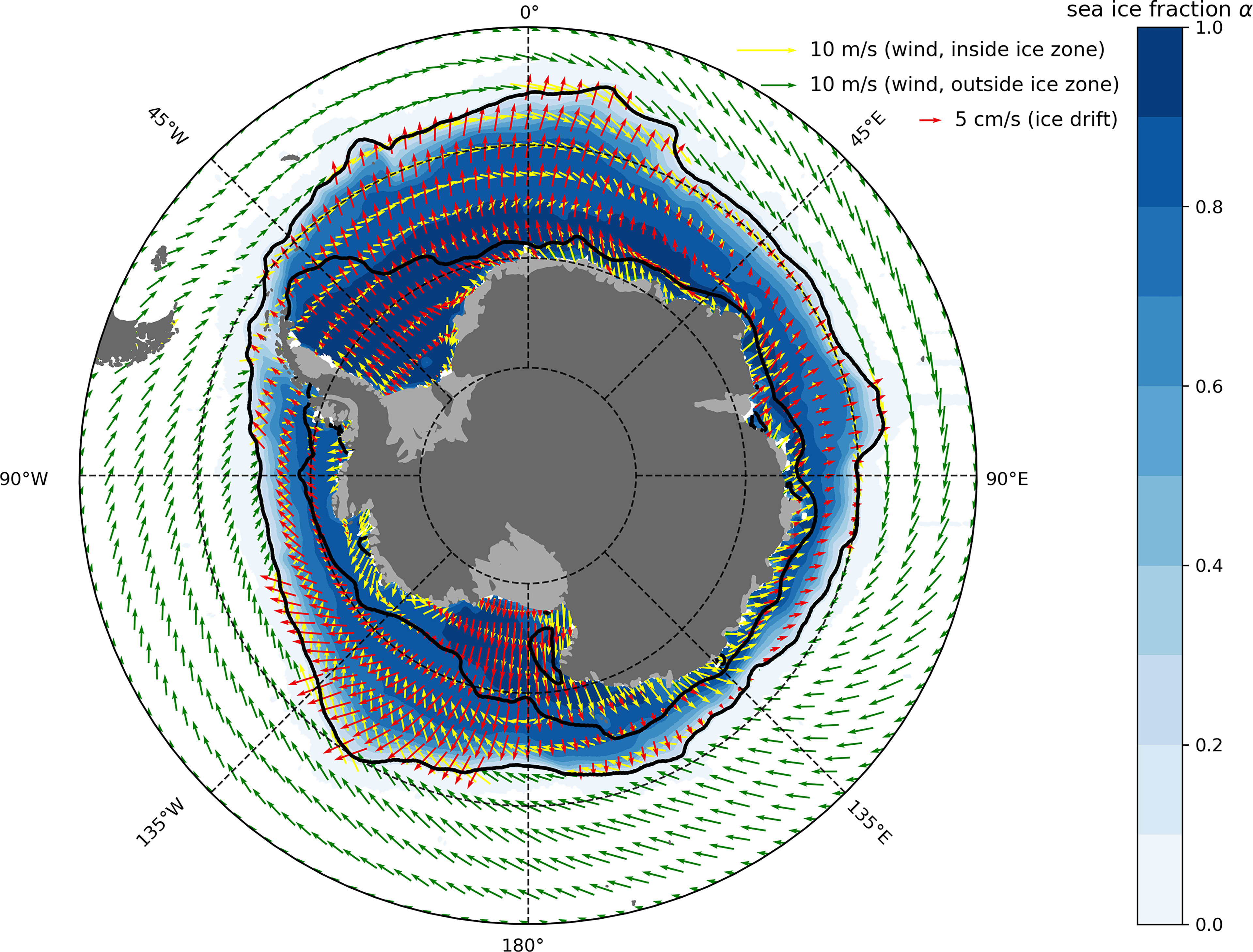
Figure 1 Key observations in the Antarctic SIZ for the austral winter months (JAS) for the period 2011–2016. Sea ice fraction α is contoured and shaded in blue. The 10m wind velocity vector field is plotted using green arrows outside the SIZ and yellow arrows inside the SIZ (the arrows inside the ice zone are twice the length as the arrows outside the ice zone for clarity). The sea ice drift velocity vector field is plotted using red arrows. The two black contours indicate the climatological positions of the September (maximum extent) and February (minimum extent) sea ice edge as defined by the location of 15% sea ice fraction contour.

Previous studies of the climatological state of the upper ocean around Antarctica, such as those by Abernathey et al. (2016) and (Pellichero et al. 2017; 2018), have taken a buoyancy budget and water transformation perspective, with an emphasis on the role of freshwater and sea-ice formation/export in sustaining the upper cell of the MOC. There has also been important work on trends in circumpolar properties. Holland and Kwok (2012) report on wind-driven trends in Antarctic sea ice drift in the context of the slight areal expansion of Antarctic sea ice cover in recent decades. Haumann et al. (2016) explores the role of sea ice transport in driving Southern Ocean salinity and its recent trends, which are among the most prominent signals of climate change in the global ocean. In this study we bring in a dynamical perspective by exploring the important role of winds and particularly sea ice which, in the SIZ, mediates the stress imparted by the winds to the underlying ocean. We use observations of surface winds, sea ice fraction, sea ice drift velocity, and geostrophic ocean currents, to estimate the stress applied to the ocean surface in the SIZ both by the surface wind and the motion of the ice driven by those winds. The resulting fields help us to map out the geography of the Antarctic Divergence zone, Ekman transport, and Ekman pumping rates in the SIZ.

In a recent observational study of the Beaufort Gyre of the Arctic ocean by (Meneghello et al. 2017; 2018), the presence of surface geostrophic flow had a marked effect on estimates of ice-ocean stress. There, sea ice, driven by the wind, drags the ocean along and the ocean currents ‘catch the ice up’, reducing the ice-ocean stress. This feedback between ice drift and surface currents was dubbed the ‘ice-ocean governor’. The Antarctic is rather different from the Arctic in that the sea-ice is thinner (order 1m) than the multi-year ice that grows in the closed basin of the Arctic Ocean, and is generally more mobile and loosely packed. Nevertheless one might expect that, as in the Arctic, estimates of stress in the SIZ could be very different if surface geostrophic currents are taken in to account. Our study can also be considered to be an extension of the regional mapping of Dotto et al. (2018) in the Ross Gyre. They assess its circulation using satellite altimetry and compute the surface stress and stress curl acting on the gyre, but do not consider the role of surface geostrophic flow or take a circumpolar view.

Our paper is set out as follows. In section 2 we describe the observational datasets used and the manner in which the data is processed. In section 3 we present maps of surface ocean stresses in the SIZ taking into account the effect of the surface ocean geostrophic flow rubbing against the ice in modulating the surface stress. In section 4 we present maps of Ekman pumping rates including its seasonal cycle. In section 5 we discuss some of the implications of our study and conclude.

2 Observational Data and Methods

Figure 1 (data sources used are described in detail below) shows key observations of the July-August-September (JAS) mean surface winds, sea ice drift velocity, and sea ice fraction, together with the position of the summer and winter ice edges around Antarctica. We see the generally eastward surface winds blowing over the open ocean to the north (green arrows). The winds continue to blow eastward as one enters the SIZ (yellow arrows), but change over to westward right in to Antarctica. The red arrows show the observed ice drift. Note how the ice is generally moving northward close in to Antarctica, but swings around in a clockwise sense to acquire a slight eastward component further out. The ice fraction (shaded in blue) reveals complete ice cover close to Antarctica which decays to zero in the open ocean north of the winter ice edge. Daily values of these fields are used to compute the stress acting on the ocean, directly from the wind in the open ocean, and through the motion of the ice over the interior ocean in the SIZ. The method we used is now described.

We follow the approach of (Yang 2006; 2009) and Meneghello et al. (2017) where the surface ocean stress τ is estimated using a linear combination of the ice-ocean and air-ocean stresses weighted by the observed local sea ice fraction 0 ≤ α ≤ 1:

$\begin{array}{ll}\tau =\alpha {\mathit{\tau }}_{io}+\left(1-\alpha \right){\mathit{\tau }}_{ao}& (1)\end{array}$

Here the ice-ocean stress τ_io and the atmosphere-ocean stress felt between sea ice floes τ_ao are computed using the following quadratic bulk drag laws

$\begin{array}{ll}\begin{array}{cc}{\mathit{\tau }}_{io}={\rho }_o{C}_{io}\left|{\mathit{u}}_r\right|{\mathit{u}}_r,& {\mathit{\tau }}_{ao}={\rho }_a{C}_{ao}\left|{\mathit{u}}_a\right|{\mathit{u}}_a\end{array}& (2)\end{array}$

where ρ_a = 1.25 kg m^-3 and ρ_o = 1027.5 kg m^-3 are atmospheric air and surface ocean water densities (assumed constant), respectively. The ice-ocean drag coefficient C_io varies considerably, by over an order of magnitude, due to under-ice topography and other factors (Cole et al., 2014). However, in the absence of the observational data required to diagnose C_io we will assume a constant C_io = 0.0055 to facilitate comparisons with previous studies and which was found to be close to the modal value obtained in the observational study of Cole et al. (2014). The air-ocean drag coefficient C_ao depends on the sea ice fraction, and thus the season, as well as the surface morphology (Lüpkes et al., 2012); however we again assume a constant C_io = 0.00125 (Lüpkes and Birnbaum, 2005) following previous studies. The 10m atmospheric wind velocity vector is denoted by u_a while u_r is the relative velocity between the ice and ocean

$\begin{array}{ll}{\mathit{u}}_r={\mathit{u}}_i-{\mathit{u}}_o=\{\begin{array}{ll}{\mathit{u}}_i-{\mathit{u}}_e,\hfill & \text{if}\hspace{0.17em}\text{geostrophic}\hspace{0.17em}\text{currents}\hspace{0.17em}\text{are}\hspace{0.17em}\text{neglected}\hfill \\ {\mathit{u}}_i-\left({\mathit{u}}_e+{\mathit{u}}_g\right),\hfill & \text{if}\hspace{0.17em}\text{geostrophic}\hspace{0.17em}\text{currents}\hspace{0.17em}\text{are}\hspace{0.17em}\text{included}\hfill \end{array}& (3)\end{array}$

where u_o is the surface ocean velocity, u_i is the sea ice drift velocity, u_e is the Ekman velocity, and u_g is the geostrophic ocean current velocity. Note how the ocean velocity [(10 cm/s), see Figure 3] is neglected with respect to the much larger wind velocity [(10 m/s) , see Figure 1], but not with respect to the comparable ice velocity [(10 cm/s), also see Figure 3].

We make two choices for the reference ocean velocity; first we set u_o = u_e and later include surface geostrophic current effects, u_o = u_g + u_e. To estimate the Ekman component of the surface ocean velocity we use the surface Ekman velocity (which is 45° to the left of the surface stress in the Southern Hemisphere)

$\begin{array}{ll}{\mathit{u}}_{\mathit{e}}\left(z=0\right)=\frac{\sqrt{2}{e}^{-i\pi /4}}{f{\rho }_o{D}_e}\mathit{\tau },& (4)\end{array}$

where f is the Coriolis parameter and we assume a fixed Ekman layer depth D_e = 20 m following previous studies: see (Yang, 2006; Yang, 2009).¹

Equations (1)–(4) form a nonlinear system of equations for τ and u_e, which we solve using the stationary (or modified) Richardson iteration with constant parameter [see Richardson (1911) for the original description and Ryaben’kii and Tsynkov (2006) for a modern treatment]. Using a Richardson relaxation parameter of 0.01 the procedure always converges after (10) iterations within an absolute tolerance of | τ^(k)−τ^(k−1) |< 10⁻⁵N m⁻² where τ^(k) is the iterate produced at iteration k.

In the above procedure we must make use of several observational datasets. The 10 m atmospheric surface winds u_a are obtained from the National Center for Environmental Prediction/National Center for Atmospheric Research (NCEP/NCAR) Reanalysis 1 (Kalnay et al., 1996). Observations of sea ice fraction, α, are obtained from the Nimbus-7 SMMR and DMSP SSM/I-SSMIS Passive Microwave Data Version 1 (Cavalieri et al., 1996). Sea ice velocity vectors u_i are obtained from the Polar Pathfinder Daily 25 km EASE-Grid Sea Ice Motion Vectors version 3 (Tschudi et al., 2016)². When used, geostrophic ocean current velocities u_g are obtained from monthly composites of dynamic ocean topography and sea level anomalies from CryoSat-2 covering both the ice-covered and ice-free regions of the Southern Ocean spanning 2011–2016 (Armitage et al., 2018)³. Observations of neutral density γⁿ, averaged over the mixed layer are obtained from monthly climatological fields produced using ship observations, Argo floats, and animal-borne sensors (mainly Southern elephant seals) (Pellichero et al., 2017; Pellichero et al., 2018). Before going on we should note that a number of atmospheric reanalysis products are available, but we chose NCEP/NCAR not least because it was the one used in deriving sea-ice velocity estimates.

Daily surface stress and Ekman transport fields are calculated on a 0.25° × 0.25° latitude-longitude grid from 40°S to 80°S over the period 2011–2016. To facilitate this calculation the individual daily data sets are linearly interpolated onto a 0.25° × 0.25° latitude-longitude grid. Climatologies are computed by summing the daily fields and dividing by the number of days of available data at each geographical position. We now present and describe the resulting maps of surface ocean stress.

3 Distribution of Surface Stresses Acting on the Ocean

3.1 Stresses Neglecting Geostrophic Currents

Figure 2 shows a winter climatology (JAS) of the surface ocean stress in the absence of geostrophic ocean currents, corresponding to an ocean velocity u_o = u_e where u_e is given by equation (4). Note that the zonal component of the surface stress dominates outside the sea ice zone, a consequence of the prevailing zonal westerlies, while both the zonal and meridional components of the ice-ocean stress are important in the SIZ. Typical stress magnitudes in the SIZ are 0.1 N m^-2.

FIGURE 2

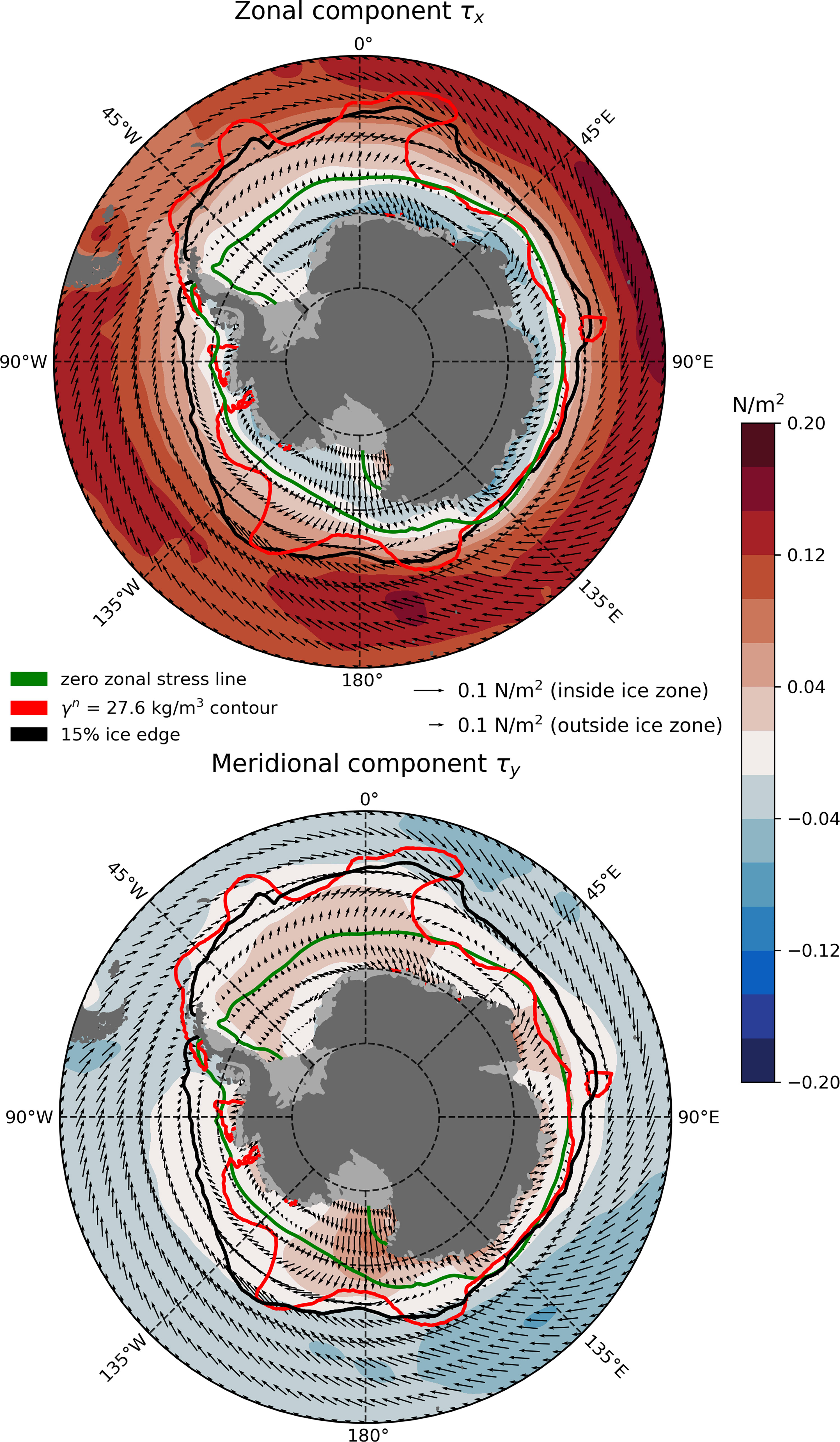
Figure 2 Winter (JAS) climatologies of the zonal (top) and meridional (bottom) components of the surface ocean stress τ over the period 2011–2016. Eastward zonal stresses and northward meridional stresses are positive. The green contour indicates the zero zonal stress line while the black contour indicates the sea ice edge as defined by the location of 15% sea ice fraction contour. The red contour indicates the position of the γⁿ = 27.6 kg m^-3 neutral density contour averaged over the mixed layer. These surface stress fields are calculated assuming no geostrophic ocean currents (u_o = u_e) .

The zonal component of surface ocean stress changes sign from eastward to westward between the ice edge and the Antarctic continent. We define this as the Divergence line, and is marked by the thick green line shown in Figure 2. This Divergence line exists almost everywhere around the Antarctic continent except at the Antarctic Peninsula, and circumscribes the Antarctic continent well within the SIZ, typically 500 km off shore. As the Divergence line lies between the Antarctic continent and the ice edge, its position consequently varies with the seasonal ice cycle. Figure 2 (top) shows that close to the Antarctic coast, the stress is directed westward (blue shading in the figure) and drives flow westwards. North of the Divergence, the stress is eastward.

The red line shown in the two panels of Figure 2 is the climatological position of the γⁿ = 27.6 kg m^-3 neutral density contour as it outcrops into the mixed layer. Marshall and Speer (2012) argue that this can be taken as the separatrix between the upper and lower cells. Note that there is very rough correspondence between the outcrop and the Divergence line around Antarctica except in the region of the Weddell and Ross Sea gyres where it meanders considerably. We now include geostrophic ocean currents in our estimates and discuss their effect on modulating the surface ocean stress field.

3.2 Effect of Surface Geostrophic Currents

Figure 3 shows winter climatologies of the zonal and meridional components of both the geostrophic current velocity u_g and the sea ice drift velocity u_i. Note that the geostrophic ocean current field, even in the climatological mean, exhibits a high frequency meridional variability. This is due perhaps to the dominant presence of mesoscale eddies in the Southern Ocean and the meandering path of the ACC, or perhaps it is the effect of the bathymetry on the ACC. In the SIZ, the geostrophic ocean currents are slower than outside the SIZ but u_g and u_i are of roughly the same magnitude. The ice velocity field exhibits a more robust pattern: eastward zonal drift in the northern half of the SIZ and westward zonal drift in the southern half of the SIZ following the wind patterns (Figure 1) which tend to blow the ice around. The sea ice drifts northward in the climatological mean. This is to be expected from a simple picture of sea ice forming near the Antarctic continent, being blown northward by the wind patterns, and melting near the ice edge where sea surface temperatures are above freezing.

FIGURE 3

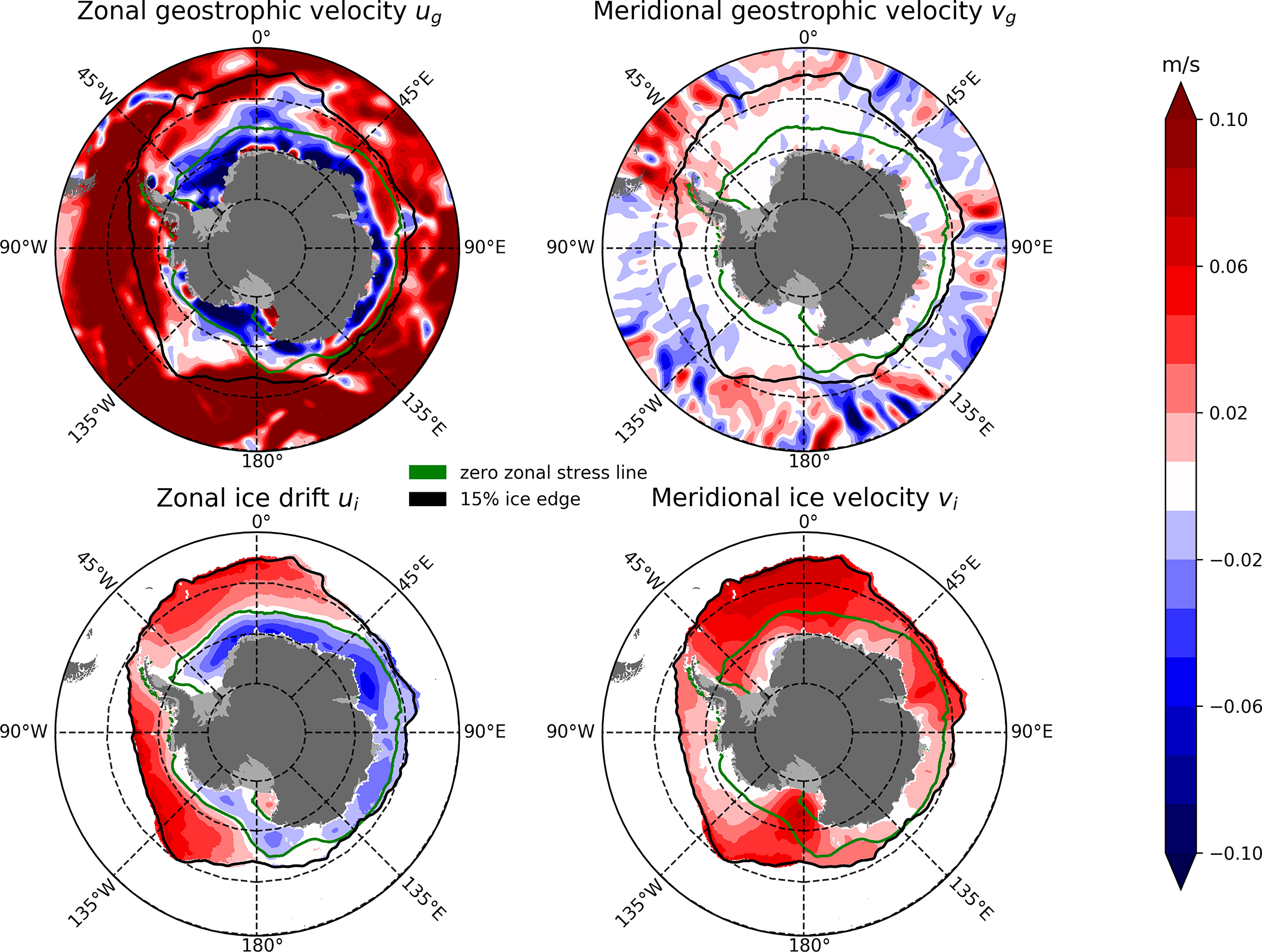
Figure 3 Winter (JAS) climatologies of the zonal (top left) and meridional (top right) components of the geostrophic current velocity u_g over the period 2011–2016, and the zonal (bottom left) and meridional (bottom right) ice drift velocities u_i over the period 2011–2016. Eastward zonal velocities and northward meridional velocities are positive. The green contour indicates the zero zonal stress line while the black contour indicates the sea ice edge as defined by the location of 15% sea ice fraction contour. The geostrophic ocean velocity fields have been smoothed using a 5-point 2D box filter.

With the inclusion of its geostrophic component, the surface ocean current is u_o = u_e + u_g. The geostrophic currents affect the surface ocean stress within the SIZ where the speed of ocean currents and ice drift are comparable. The resulting surface ocean stress fields are presented in Figure 4. The inclusion of the geostrophic currents introduces additional spatial structure to the surface ocean stress field which in turn complicates the position of the Divergence line. The line is less distinct than before and meanders in position within the SIZ, often moving right in toward the coast. This is evidence of the ice-ocean governor in action around Antarctica, a consequence of the ocean currents and sea-ice having comparable speeds, resulting in the frequent vanishing of the ice-ocean stress.

FIGURE 4

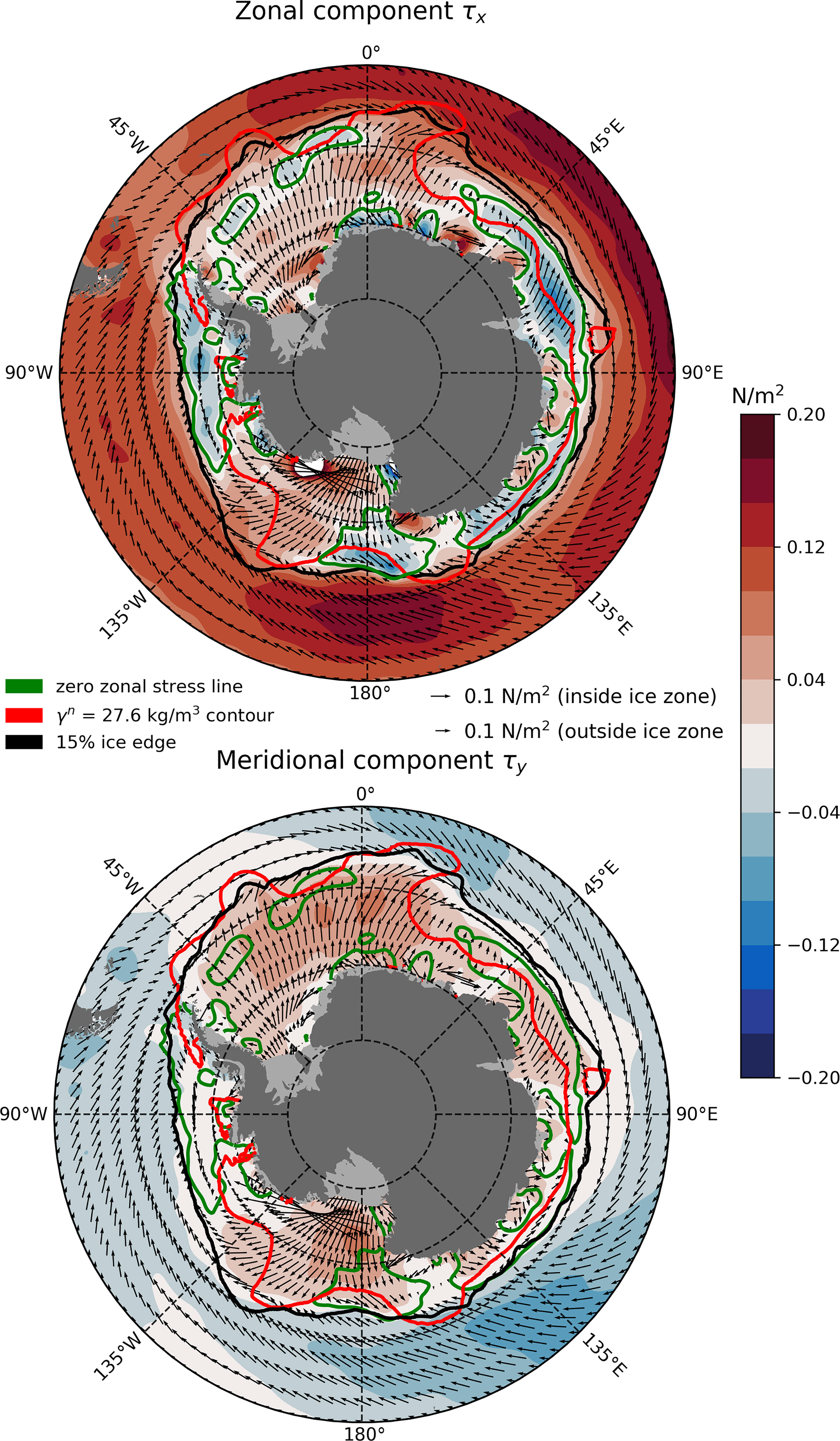
Figure 4 Same as Figure 2 but using climatological geostrophic ocean currents (u_o = u_e + u_g) The fields have been smoothed using a 5-point 2D box filter.

4 Pattern of Ekman Currents and Associated Ekman Pumping

Maps of the winter-mean (JAS) Ekman transport U_e, which is 90° to the left of the surface stress in the Southern Hemisphere,

$\begin{array}{ll}{\mathbf{U}}_e={\displaystyle {\int }_0^{\infty }{\mathbf{u}}_e\left(z\right)dz}=\frac{1}{f{\rho }_o}\left(\begin{array}{c}{\tau }_y\\ -{\tau }_x\end{array}\right)& (5)\end{array}$

are presented in Figure 5. We see a northward Ekman transport north of the Divergence, and a southward transport south of the Divergence. This is particularly clear in Figure 5 (left) where the effect of the underlying ocean circulation is not included. When such effects are included, however, as in Figure 5 (right), the large-scale pattern remains largely the same, albeit with more small-scale variation. The meridional component of the Ekman transport dominates outside the SIZ. Both zonal and meridional Ekman components are equally important in the SIZ where the flow is weaker and predominantly towards the southwest, as expected from an inspection of the surface stress maps (the mean Ekman transport is 90° to the left of the surface stress).

FIGURE 5

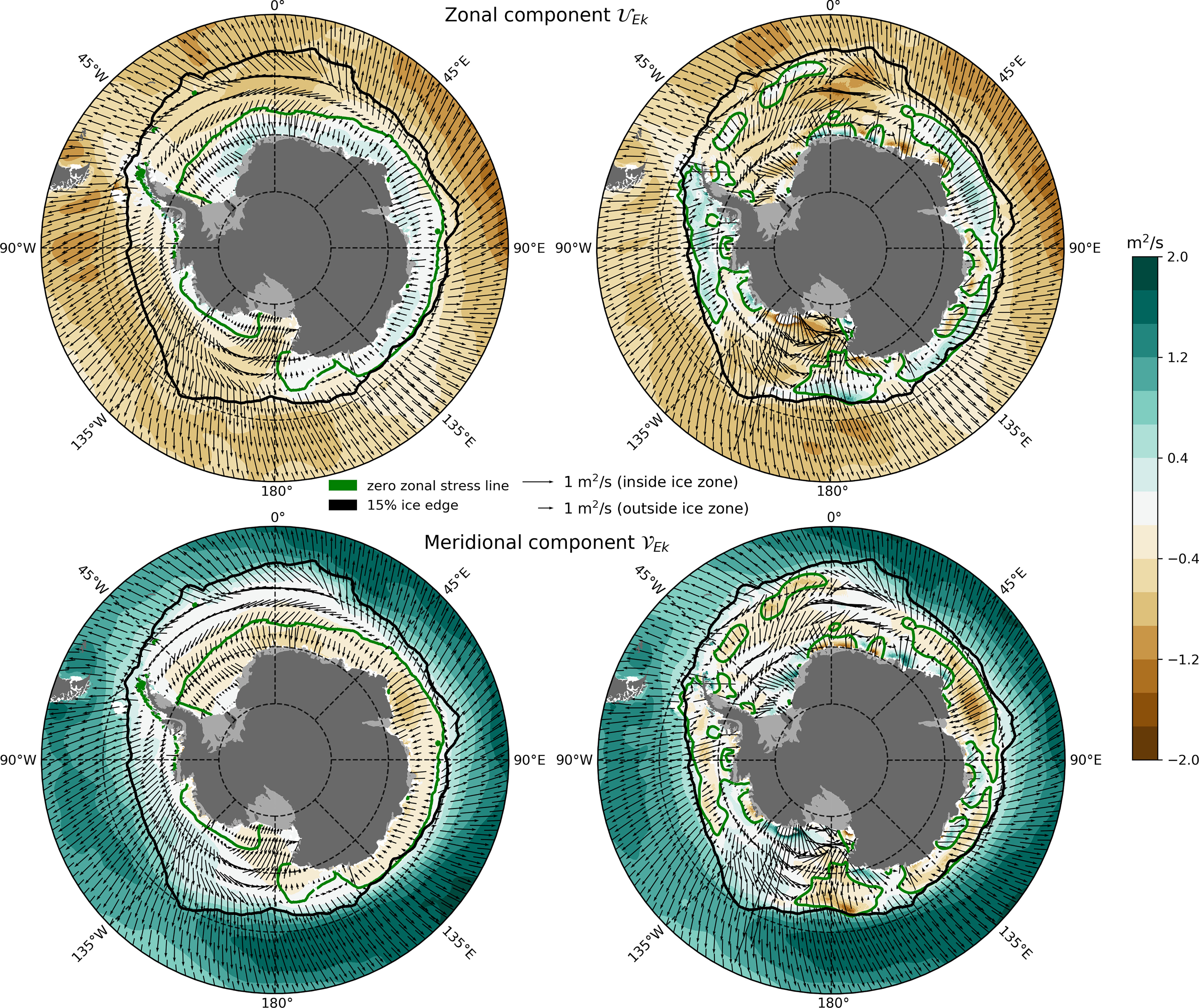
Figure 5 Winter (JAS) climatologies of the zonal (top) and meridional (bottom) components of the Ekman transport U_e with over the period 2011–2016. The left hand column shows the case where u_g = 0 and the right hand column where u_i is included in the calculation. As before, the green contour indicates the zero zonal stress line while the black contours indicate the minimum and maximum extent of the sea ice edge as defined by the location of 15% sea ice fraction contour. The fields plotted on the right have been smoothed using a 5-point 2D box filter.

The Ekman pumping rate

$\begin{array}{ll}{w}_e=\nabla \times \left(\frac{\mathit{\tau }}{{\rho }_{o}f}\right)& (6)\end{array}$

associated with the ocean surface stress in the Southern Ocean is plotted in Figure 6 in the absence and presence of geostrophic ocean currents. The maps reveal large-scale upwelling within the SIZ but with many smaller-scale features appearing where the effect of ocean currents is of importance. It should be noted that equation (6) assumes that the Rossby number is small, allowing neglect of the contribution of the relative vorticity considered by Stern (1965) and Gaube et al. (2015). Computation of the Rossby number from the monthly-mean surface geostrophic currents (not shown) indicates that this is indeed small (less than 0.1) in the seasonal ice zone, at the resolution of the available data. Thus equation 6 is a very good approximation.

FIGURE 6

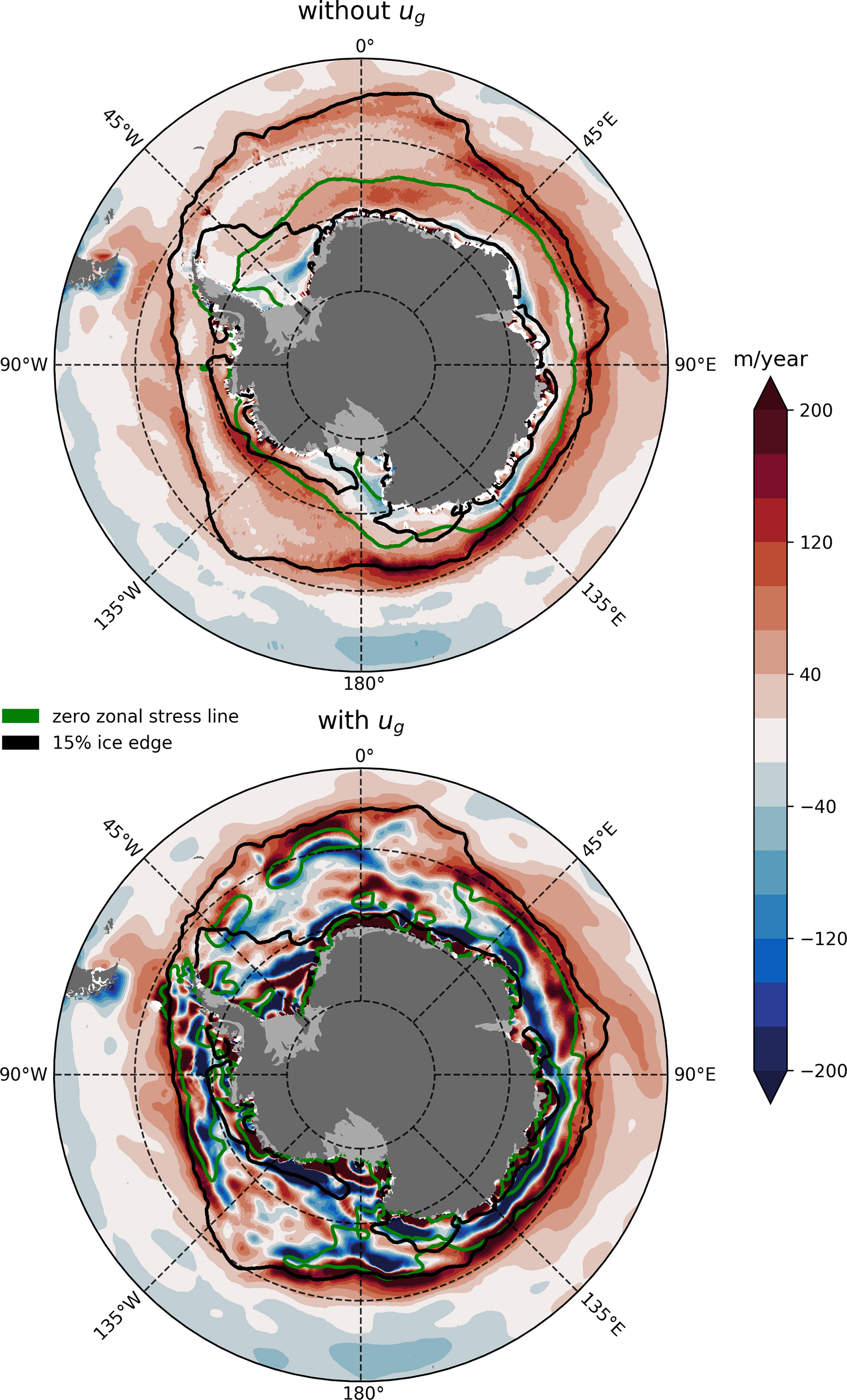
Figure 6 Winter (JAS) climatologies of Ekman pumping in the absence of geostrophic ocean currents (top) and with their inclusion (bottom) over the period 2011–2016. The green contour indicates the zero zonal stress line while the black contours indicates the minimum and maximum sea ice edge as defined by the location of 15% sea ice fraction contour. The plot on the bottom has been smoothed using a 5-point 2D box filter.

A striking feature, appearing both in the absence and presence of geostrophic ocean currents, is the zone of upwelling that follows the sea ice edge being especially prominent in the Eastern Hemisphere. A sharp decrease in sea ice fraction (Figure 1), and thus in the ice-ocean stress, occurs as the ice edge is traversed northward, which in turn produces a large divergence of stress at the ocean surface around the ice edge bringing up ocean water from depth. A second feature, prominent in the absence of geostrophic ocean currents, is a second zone of upwelling closely following the zero zonal stress line. This is where the zonal component, and to a lesser extent the meridional component, of the surface stress (Figure 2), changes sign and produces a large gradient in the surface stress perpendicular to the zero zonal stress line, again leading to a divergence of stress and subsequent upwelling. Note how, in the presence of u_g, Ekman pumping has changed sign — from upwelling to downwelling — over large parts of the Weddell Sea. There is also a region of pronounced downwelling all the way around the continental margin which is almost entirely absent when the effects of ocean currents are neglected.

In summary, then, in the presence of surface ocean currents, the SIZ is a region of large-scale upwelling in the wintertime with typical values of 40 m yr^-1 which is intensified to values in excess of 100 m yr^-1 near the ice edge. This is balanced by a circumpolar band of intense downwelling adjacent to the boundary where rates in excess of 200 m yr^-1 are found.

Figure 7 shows the Ekman pumping field season by season. Note that in the top left panel (already presented in Figure 6) the SIZ is at its largest winter extent (JAS). The spring pattern (OND) is broadly similar with upwelling over the outer flank of the SIZ, with downwelling on the inside. In the summer (JFM) ice has been replaced by open ocean and there is broad upwelling over almost all of the circumpolar domain. Downwelling in the inner circumpolar domain returns in the fall (AMJ). The ice edge in all seasons coincides with a region of strong upwelling, a consequence of the change of the stress across the ice edge, inducing a large curl.

FIGURE 7

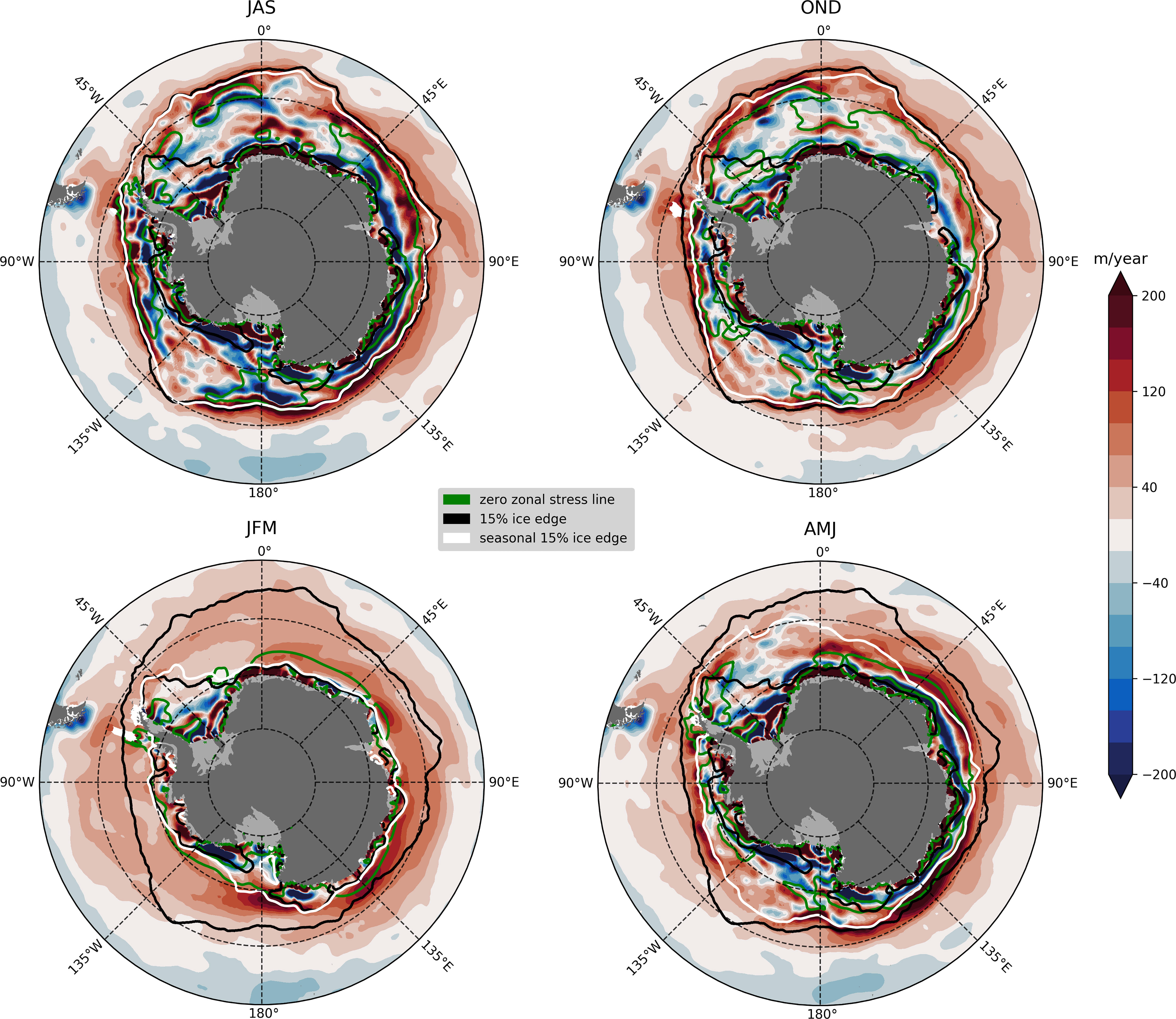
Figure 7 Seasonal cycle of Ekman pumping including the effect of geostrophic ocean currents averaged over the period 2011–2016. Clockwise from top left: JAS, OND, JFM and AMJ. Red indicates upwelling and blue downwelling. The green contour indicates the zero zonal stress line while the black contours indicates the minimum and maximum sea ice edge as defined by the location of 15% sea ice fraction contour. The white contour marks the ice edge in that season. The fields plotted have been smoothed using a 5-point 2D box filter.

For completeness, Figure 8 shows the annual mean climatology of zonal surface stress and Ekman pumping. The main patterns of the winter (JAS) mean Ekman pumping field — distributed upwelling over the SIZ balanced by intense downwelling around the continent — imprint themselves on the annual mean, but amplitudes are diminished due to the temporal averaging. The Divergence meanders considerably over the SIZ, often approaching the Antarctic margin. Thus ice-ocean effects appear to be important in climatological means, not just in the winter season.

FIGURE 8

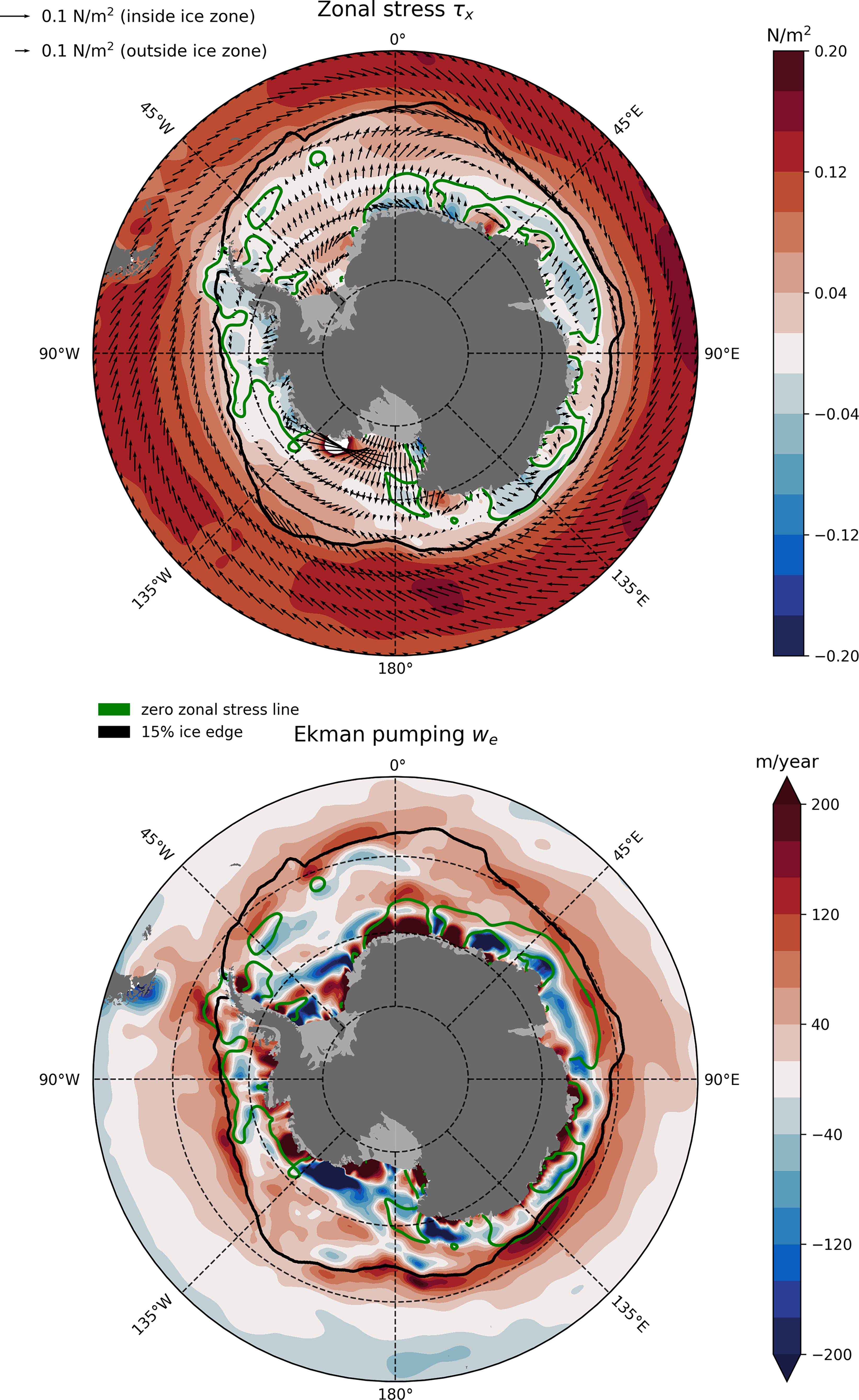
Figure 8 (Top) Similar to Figure 4 but showing an annual mean climatology of zonal surface stress. (Bottom) Similar to Figure 7 but showing an annual mean climatology of Ekman pumping. The fields plotted have been smoothed using a 5-point 2D box filter.

5 Discussion and Conclusions

We have attempted to infer from observations patterns of stress applied by atmospheric winds to the ocean below, as mediated by the presence of ice in the SIZ around Antarctica. Unlike previous studies, for example the regional study of Dotto et al. (2018), we have explored the role of surface geostrophic currents in setting the amplitude and pattern of Ekman pumping and brought a circumpolar Antarctic perspective.

Our main conclusions are:

1. If surface currents are neglected, the climatological position of the Antarctic Divergence in JAS (the line at which the zonal stress changes sign) is contiguous and circumnavigates the globe roughly 500 km off shore, within the SIZ.

2. Inclusion of surface geostrophic currents makes a zero-order contribution to estimates of surface stress and Ekman pumping. The Antarctic Divergence is no longer contiguous or organized, but instead meanders within the SIZ. This is because surface current speeds approach that of the drifting sea-ice above, tending to ‘turn off’ the ice-ocean stress. In this sense there is a generalised ‘ice-ocean governor’ in operation around Antarctica in which surface currents and sea-ice drifts are comparable to one-another.

3. The SIZ is found to be a region of generalised upwelling, typically 40 m yr^-1, enhanced near the sea-ice edge where it can exceed 100 m yr^-1. This is balanced by a band of intense downwelling close in to the boundary, all the way around Antarctica, which can reach several 100 m yr^-1.

Finally, the current study is suggestive of several lines of further enquiry to answer questions that stem from it. What are the uncertainties in our estimates and do similar patterns emerge if different reanalysis products are used? If true, what are the consequences for the large-scale ocean circulation of the new and rather different Ekman pumping patterns presented here? The geostrophic gyre structure as revealed by altimetry ought to reflect the actual forcing which must include the sea-ice influences explored here. Are monthly geostrophic currents consistent with the implied geostrophic flow due to the (modified) integrated wind stress curl? Can we connect the wind driven upwelling, particularly near the ice edge, to heave or vertical motion of isopycnals from Argo data? All these and more would seem to be valuable areas for future enquiry.

Data Availability Statement

The datasets presented in this study can be found in online repositories. The datasets used are described and referenced in section 2.

Author Contributions

JM conceived and designed the study. AR performed the analysis, prepared the figures, and wrote the first draft of the manuscript. All authors contributed to the interpretation of the results. All authors contributed to manuscript revision, read, and approved the submitted version.

Funding

We would like to thank endowed funds at MIT for partial support of the work described here and also the Physical Oceanography program of NASA.

Conflict of Interest

The authors declare that the research was conducted in the absence of any commercial or financial relationships that could be construed as a potential conflict of interest.

Publisher’s Note

All claims expressed in this article are solely those of the authors and do not necessarily represent those of their affiliated organizations, or those of the publisher, the editors and the reviewers. Any product that may be evaluated in this article, or claim that may be made by its manufacturer, is not guaranteed or endorsed by the publisher.

Acknowledgments

We thank Edward Doddridge for helpful discussions during the early stages of this work. We also thank the three reviewers for their very helpful comments.

Footnotes

1. ^ These previous studies investigated the dynamics of the Arctic Ocean. We assume the same value of D_e pertains in the Southern Ocean.
2. ^ Persistent Eulerian and Lagrangian artifacts have been found in this dataset related to the incorporation of buoy data which especially impacts the Arctic. This mainly impacts the evaluation of sea ice motion gradients (Szanyi et al., 2016)
3. ^ Armitage et al., (2018) identify north-south striping artifacts in the sea level anomaly field, but these seem to be confined to the region of the Weddell Gyre.

References

Abernathey R. P., Cerovecki I., Holland P. R., Newsom E., Mazloff M., Talley L. D. (2016). Water-Mass Transformation by Sea Ice in the Upper Branch of the Southern Ocean Overturning. Nat. Geosci. 9 (8), 596–601. doi: 10.1038/ngeo2749

CrossRef Full Text | Google Scholar

Armitage T. W. K., Kwok R., Thompson A. F., Cunningham G. (2018). Dynamic Topography and Sea Level Anomalies of the Southern Ocean: Variability and Teleconnections. J. Geophys. Res.: Ocean. 123 (1), 613–630. doi: 10.1002/2017JC013534

CrossRef Full Text | Google Scholar

Cavalieri D. J., Parkinson C. L., Gloersen P., Zwally H. J. (1996). Sea Ice Concentrations From Nimbus-7 SMMR and DMSP SSM/I-SSMIS Passive Microwave Data, Version 1. Boulder. Colorad. U. S. A. NASA. Natl. Snow. Ice. Data Cent. Distrib. Act. Arch. Cent. doi: 10.5067/8GQ8LZQVL0VL

CrossRef Full Text | Google Scholar

Cole S. T., Timmermans M.-L., Toole J. M., Krishfield R. A., Thwaites F. T. (2014). Ekman Veering, Internal Waves, and Turbulence Observed Under Arctic Sea Ice. J. Phys. Oceanogr. 44 (5), 1306–1328. doi: 10.1175/JPO-D-12-0191.1

CrossRef Full Text | Google Scholar

Deacon G. E. (1933). A General Account of the Hydrology of the South Atlantic Ocean. Discovery Rep. 7, 171–238.

Google Scholar

Deacon G. E. (1937). The Hydrology of the Southern Ocean. Discovery Rep. 15, 3–122.

Google Scholar

Dotto T. S., Naveira Garabato A., Bacon S., Tsamados M., Holland P. R., Hooley J., et al. (2018). Variability of the Ross Gyre, Southern Ocean: Drivers and Responses Revealed by Satellite Altimetry. Geophys. Res. Lett. 45 (12), 6195–6204. doi: 10.1029/2018GL078607

CrossRef Full Text | Google Scholar

Gaube P., Chelton D. B., Samelson R. M., Schlax M. G., O’Neill L. W. (2015). Satellite Observations of Mesoscale Eddy-Induced Ekman Pumping. J. Phys. Oceanogr. 45 (1), 104–132. doi: 10.1175/JPO-D-14-0032.1

CrossRef Full Text | Google Scholar

Haumann F. A., Gruber N., Münnich M., Frenger I., Kern S. (2016). Sea-Ice Transport Driving Southern Ocean Salinity and Its Recent Trends. Nature 537 (7618), 89–92. doi: 10.1038/nature19101

PubMed Abstract | CrossRef Full Text | Google Scholar

Holland P. R., Kwok R. (2012). Wind-Driven Trends in Antarctic Sea-Ice Drift. Nat. Geosci. 5 (12), 872–875. doi: 10.1038/ngeo1627

CrossRef Full Text | Google Scholar

Kalnay E., Kanamitsu M., Kistler R., Collins W., Deaven D., Gandin L., et al. (1996). The NCEP/NCAR 40-Year Reanalysis Project. Bull. Am. Meteorolog. Soc. 77 (3), 437–471. doi: 10.1175/1520-0477(1996)077<0437:TNYRP>2.0.CO;2

CrossRef Full Text | Google Scholar

Lüpkes C., Birnbaum G. (2005). Surface Drag in the Arctic Marginal Sea-Ice Zone: A Comparison of Different Parameterisation Concepts. Bound-Lay. Meteorol. 117 (2), 179–211. doi: 10.1007/s10546-005-1445-8

CrossRef Full Text | Google Scholar

Lüpkes C., Gryanik V. M., Hartmann J., Andreas E. L. (2012). A Parametrization, Based on Sea Ice Morphology, of the Neutral Atmospheric Drag Coefficients for Weather Prediction and Climate Models. J. Geophys. Res.: Atmos. 117 (D13), D13112. doi: 10.1029/2012JD017630

CrossRef Full Text | Google Scholar

Marshall J., Speer K. (2012). Closure of the Meridional Overturning Circulation Through Southern Ocean Upwelling. Nat. Geosci. 5 (3), 171–180. doi: 10.1038/ngeo1391

CrossRef Full Text | Google Scholar

Meneghello G., Marshall J., Cole S. T., Timmermans M.-L. (2017). Observational Inferences of Lateral Eddy Diffusivity in the Halocline of the Beaufort Gyre. Geophys. Res. Lett. 44 (24), 12331–12338. doi: 10.1002/2017GL075126

CrossRef Full Text | Google Scholar

Meneghello G., Marshall J., Timmermans M.-L., Scott J. (2018). Observations of Seasonal Upwelling and Downwelling in the Beaufort Sea Mediated by Sea Ice. J. Phys. Oceanogr. 48 (4), 795–805. doi: 10.1175/JPO-D-17-0188.1

CrossRef Full Text | Google Scholar

Pellichero V., Sallée J.-B., Chapman C. C., Downes S. M. (2018). The Southern Ocean Meridional Overturning in the Sea-Ice Sector is Driven by Freshwater Fluxes. Nat. Commun. 9 (1), 1–9. doi: 10.1038/s41467-018-04101-2

PubMed Abstract | CrossRef Full Text | Google Scholar

Pellichero V., Sallée J.-B., Schmidtko S., Roquet F., Charrassin J.-B. (2017). The Ocean Mixed Layer Under Southern Ocean Sea-Ice: Seasonal Cycle and Forcing. J. Geophys. Res.: Ocean. 122 (2), 1608–1633. doi: 10.1002/2016JC011970

CrossRef Full Text | Google Scholar

Richardson L. F. (1911). The Approximate Arithmetical Solution by Finite Differences of Physical Problems Involving Differential Equations, With an Application to the Stresses in a Masonry Dam. Philos. Trans. R. Soc. Lond. Ser. A. Contain. Pap. Math. Phys. Charact. 210, 307–357. doi: 10.1098/rsta.1911.0009

CrossRef Full Text | Google Scholar

Ryaben’kii V. S., Tsynkov S. V. (2006). A Theoretical Introduction to Numerical Analysis (Boca Raton, FL:Chapman and Hall/CRC.(Section 6.1).

Google Scholar

Stern M. E. (1965). Interaction of a Uniform Wind Stress With a Geostrophic Vortex. Deep. Sea. Res. Oceanogr. Abstr. 12 (3), 355–367. doi: 10.1016/0011-7471(65)90007-0

CrossRef Full Text | Google Scholar

Szanyi S., Lukovich J. V., Barber D. G., Haller G. (2016). Persistent Artifacts in the NSIDC Ice Motion Data Set and Their Implications for Analysis. Geophys. Res. Lett. 43 (20), 10800–10807. doi: 10.1002/2016GL069799

CrossRef Full Text | Google Scholar

Tschudi M., Fowler C., Maslanik J., Stewart J. S., Meier W. (2016). Polar Pathfinder Daily 25 Km EASE-Grid Sea Ice Motion Vectors, Version 3. Boulder, Colorado USA. NASA. Natl. Snow. Ice. Data Cent. Distrib. Act. Arch. Cent. doi: 10.5067/O57VAIT2AYYY

CrossRef Full Text | Google Scholar

Wyrtki K. (1960a). The Antarctic Circumpolar Current and the Antarctic Polar Front. Deutsch. Hydrograf. Z. 13 (4), 153–174. doi: 10.1007/BF02226197

CrossRef Full Text | Google Scholar

Wyrtki K. (1960b). The Antarctic Convergence–and Divergence. Nature 187, 581–582. doi: 10.1038/187581a0

CrossRef Full Text | Google Scholar

Yang J. (2006). The Seasonal Variability of the Arctic Ocean Ekman Transport and its Role in the Mixed Layer Heat and Salt Fluxes. J. Climate 19 (20), 5366–5387. doi: 10.1175/JCLI3892.1

CrossRef Full Text | Google Scholar

Yang J. (2009). Seasonal and Interannual Variability of Downwelling in the Beaufort Sea. J. Geophys. Res.: Ocean. 114 (C1), C00A14.doi: 10.1029/2008JC005084

CrossRef Full Text | Google Scholar