Movements and diving behavior of Risso’s dolphins in the Southern California Bight

Introduction

Risso’s dolphins (Grampus griseus, hereafter referred to as “Risso’s”) are a medium-sized, cosmopolitan odontocete found in temperate and tropical waters. They typically occur between latitudes 60°N to 60°S where sea surface temperatures are greater than 10°C; however, the highest numbers of individuals are found between 30° and 45° latitudes, in waters 15–20°C (Kruse et al., 1999; Baird, 2002; Jefferson et al., 2014b). In the eastern Pacific, Risso’s are abundant and widely dispersed year-round (Leatherwood et al., 1980). They can be found as far north as the Gulf of Alaska and south to Tierra del Fuego (Baird, 2002; Jefferson et al., 2014b). Risso’s are most often associated with shelf-edge and upper continental slope habitat, in areas of steep bottom topography with average depths ranging from 100 to 1000 m (Kruse, 1989; Baumgartner, 1997; Kruse et al., 1999; Baird, 2002; Cañadas et al., 2002; Jefferson et al., 2006; Azzellino et al., 2008). Although highest densities are found along this shelf/slope region, they utilize a wide range of habitats, from shallow, coastal areas (Boer et al., 2013; Jefferson et al., 2014b) to offshore pelagic waters (Baird, 2016). Group size is typically 10–50, although singletons and groups upwards of 4,000 individuals have been documented (Leatherwood et al., 1980; Baird, 2002; Baird, 2016).

Currently, the population abundance of Risso’s along the coasts of Washington, Oregon, and California is estimated at 6,336 (CV = 0.32) individuals (Carretta et al., 2020). Movement patterns within this population have been discerned through sightings and acoustic detections. It is thought that Risso’s in this region demonstrate broadscale seasonal shifts northward from California into Oregon/Washington in the spring/summer months coincident with rising water temperatures (Green et al., 1992). High inter-annual seasonal variability north of (Dohl et al., 1983; Kruse, 1989; Soldevilla et al., 2010), and year-round presence within, the Southern California Bight (Soldevilla et al., 2010), a productive oceanographic region off the coast of the southwestern United States (U.S.), have been documented. Long–term changes in the abundance and distribution of Risso’s have also been documented in the Southern California Bight. In the late 1950s, they were rarely encountered there (Norris and Prescott, 1961). Between 1972 and 1975, sightings increased in frequency as their distribution shifted inshore (Leatherwood et al., 1980). Starting in the El Niño years of 1982–83, occurrence further increased in the Bight and Santa Catalina Island was identified as particularly important habitat (Shane, 1995b). They continue to be regularly documented there both visually and acoustically (Soldevilla et al., 2010; Jefferson et al., 2014a; Bacon et al., 2017).

Risso’s have a primarily teuthophagus diet consisting of both squid and octopus (Clarke, 1996; Baird, 2002; Blanco et al., 2006; Jefferson et al., 2006; Bearzi et al., 2011; Yates and Palavecino-Sepúlveda, 2011; Bloch, 2012; Milani et al., 2017; Luna et al., 2021), though they also feed on fish and crustaceans (Reeves et al., 2002; Bloch, 2012). With the exception of octopus in the western Mediterranean (Blanco et al., 2006), squid appear to be their preferred cephalopod prey (Clarke, 1996; Bearzi et al., 2011; Yates and Palavecino-Sepúlveda, 2011; Bloch, 2012). In California waters, some species of squid that have been identified as important prey for Risso’s, including jumbo squid (Dosidicus gigas) (Orr, 1966; Gilly et al., 2006) and market squid (Loligo opalescens) (Kruse, 1989), perform diurnal vertical migrations (Watanabe et al., 2006). These species serve as both prey and predators within the ecosystem, feeding on deep-, mid-, and shallow-water organisms such as krill and other crustaceans, small fish, and even other cephalopods, with observations suggesting they may feed at the surface in the early evening (Markaida and Sosa-Nishizaki, 2003). Jumbo squid in particular have demonstrated daytime depths exceeding 250 m, near-surface depths at dusk, and variable depths throughout the night (Gilly et al., 2006).

Our understanding of foraging behavior of Risso’s has advanced markedly in recent years. Initial observational studies suggested Risso’s rested or traveled during the day and foraged at night (Shane, 1995b). An increase in both click rates and bouts at night suggested Risso’s foraging activity is related to diurnal patterns in squid behavior (Soldevilla et al., 2010). Most recent work indicates that Risso’s perform foraging dives during the day as well as at night (Benoit-Bird et al., 2017; Arranz et al., 2018; Benoit-Bird et al., 2019) with maximum depths exceeding 500 m particularly common during the day (Benoit-Bird et al., 2019). They regularly switch predation tactics between a near-surface generalist and deep-water squid specialist even within a single dive (Benoit-Bird et al., 2019). They plan foraging dives based on knowledge attained on previous dives (Arranz et al., 2018, Visser et al., 2021) and use a spin dive strategy to decrease transit time to exploit the diurnal mesopelagic layer (Visser et al., 2021).

Reliable assessments of Risso’s movements and diving behavior are challenging yet essential for understanding population structure, stock boundaries, habitat use, and potential exposure to anthropogenic impacts. Satellite tags can provide a more objective, detailed depiction of individual movements and behavior than visual or acoustic surveys alone. As part of a long-term research effort to examine cetacean movements, habitat use, and ecology within the Southern California Bight, we remotely deployed 16 Argos-linked satellite tags on Risso’s between 2009 and 2019, and here report on habitat use, dive behavior, and movements of these tagged individuals.

Materials and methods

Data collection

Tag data collection and processing

Fieldwork was undertaken in the Southern California Bight, primarily off San Clemente and Santa Catalina Islands, from 2009 to 2019 (Figure 1). Satellite tags in the Low Impact Minimally Percutaneous External-electronics Transmitter (LIMPET) configuration were deployed on or near the dorsal fin using a Dan-Inject modified air rifle. Tags were affixed by two 3.4 cm medical-grade titanium barbed darts which were gas sterilized prior to attachment (Andrews et al., 2019). The tags contained either Wildlife Computers’ (Redmond, WA) SPOT5 location-only, or SPLASH10-A or SPLASH10-F location and dive reporting transmitters. The age class of each tagged individual was estimated based on the relative size and level of scarring (Kruse et al., 1999; Hartman et al., 2016).

FIGURE 1

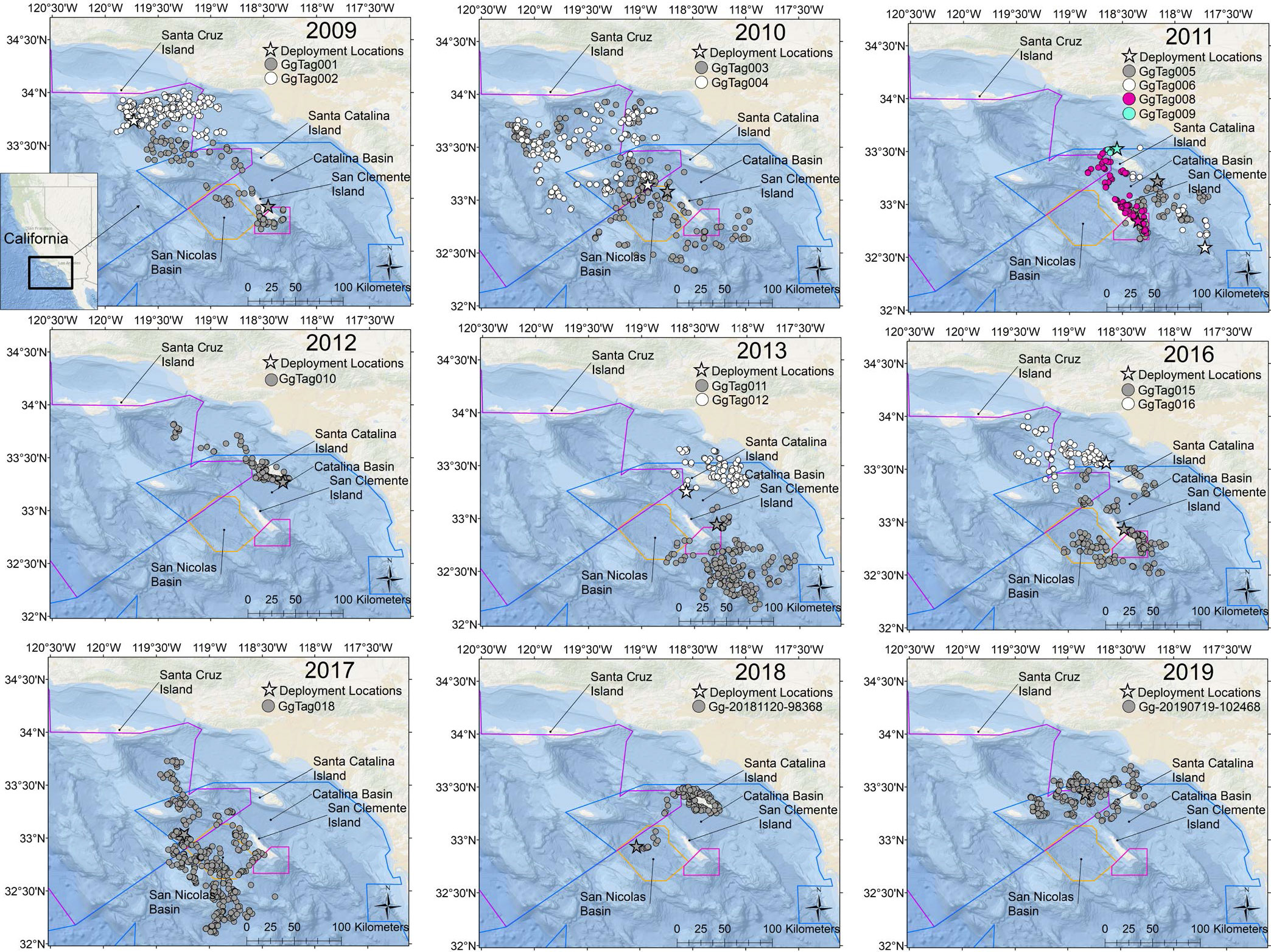
Figure 1 Maps of the study area with filtered locations of Risso’s dolphins tagged within the Southern California Bight annually. The inset shows the study area in a broader geographic context of the state of California. Range Polygons: Blue = Southern California Range Complex; Purple = Point Mugu Sea Range; Orange = Southern California Anti-submarine Warfare Range; Pink = Shore Bombardment Area.

SPLASH10-A tags transmitted a record of diving behavior in the form of a behavior log (BL). BL data were received via the Argos satellite system and from a land-based Argos receiving station (Wildlife Computers Mote) installed on San Clemente Island in 2014 (Jeanniard-du-Dot et al., 2017). BL data consisted of summarized dive and surfacing events and included event start and end times and the maximum depth of dives. As the number of tag deployments grew, our understanding of Risso’s dive behavior improved. Thus, adjustments to tag programming were made during the course of study to maximize the quantity and relevance of BL data captured while minimizing data gaps. Dive events were defined as any submergence that exceeded either 30 m (6 tags) or 50 m (2 tags) depth and lasted more than 30 s (3 tags) or 1 min (5 tags) (Table 1). Depth accuracy for the pressure transducers in these tags was independently verified in a pressure chamber to 3,000 m, resulting in a maximum error of <+/- 2.5% of the recorded value (Schorr et al., 2014). Initially, start and end times were determined by crossing the 5 m depth threshold upon descent or ascent of a qualifying dive for the first two tags. After assessment of tag performance, the next six tags were programmed with start and end times determined by the transition from wet to dry when the tag broke the surface during a typical breath, and therefore this programming regimen allowed for a more accurate assessment of dive and surfacing times (Table 1). The single SPLASH10-F tag that was deployed during this study was programmed to collect only maximum dive depth histogram data (https://wildlifecomputers.com/our-tags/splash-archiving-tags/splash10-f/) to prioritize the collection of higher resolution Fastloc GPS location data in addition to Argos location data, and thus was excluded from dive analyses.

TABLE 1

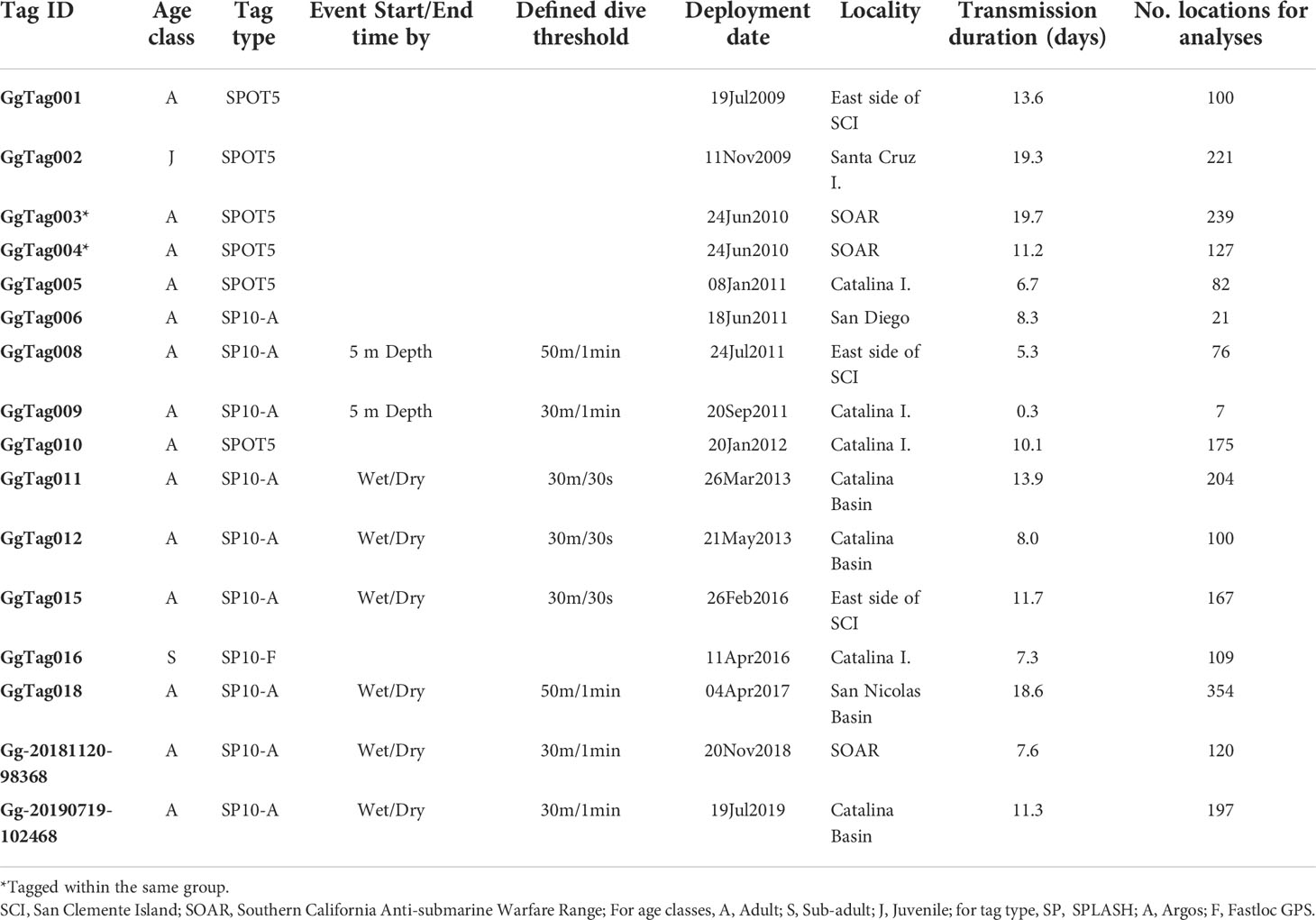
Table 1 Details of Risso’s dolphin satellite tag deployments by individual.

Locations received via Argos satellite were re-processed by Argos using the Kalman filter to improve location accuracy (Lopez et al., 2014), uploaded to Movebank (www.movebank.org), and then processed using the Douglas Argos-Filter (v10.5.2) with the ‘distance-angle-rate’ filter (Douglas et al., 2012). Filtering parameters were set as follows: maximum-redundant-distance at 3 km, maximum sustainable rate at 15 km h^-1, and the rate coefficient (the angle created by three subsequent points, Ratecoef) at the default of 25. Argos location classes 2 and 3 have an estimated error from Argos of < 500 m (Argos User’s Manual) and were automatically retained. Filtered SPLASH-10F tag Fastloc GPS locations (locations with residuals > 35 or time error > +/- 3 min removed) were combined with the tag’s Douglas-filtered Argos data to provide the highest resolution location data available for this individual. The cumulative distance traveled during each tag transmission and the straight-line distance from the deployment location were calculated using all locations that passed the filter, regardless of quality.

For dive behavior analyses, Douglas-filtered locations were fit by a continuous-time correlated random walk model (Johnson et al., 2008) that incorporated Argos ellipse errors (McClintock et al., 2015) using the crawl (v2.2.1) R package (Johnson and London, 2018; R Core Team, 2021) to estimate the animal’s position at the start time of every dive. Although standard errors ranged from 0 to 26 km for model-estimated locations, a function of Argos location qualities and time between consecutive Douglas-filtered locations, they were considered the best estimate of the animal’s position at the start time of each dive. Given these inherent sources of error or uncertainty in our spatial data, we exercised caution when interpreting results associated with data derived from both model-estimated and Douglas-filtered locations.

Environmental data collection

A series of ArcGIS layers were created containing bathymetric, remote sensing, land, and Navy range boundaries. Depth, slope, distances to nearest shore (either islands or mainland) and to the mainland, and assessment of locations within range boundaries were extracted by overlaying tag location data onto raster surfaces or in relation to polygons in ArcGIS v10.7.1 (NAD 1983 UTM Zone 11N) (ESRI, 2019). Less than 1% of location estimates were on land according to the raster surfaces—a result of poor-quality locations and Risso’s use of steep near-shore bathymetry; these were removed from subsequent movement and dive behavioral analyses. For analyses of depth and slope, only Douglas-filtered locations of qualities 2 and 3 were included, given the size of error ellipses associated with lesser quality Argos positions (Lopez et al., 2014) and the variable nature of depth and slope over a limited geographic area. Bathymetric data were obtained from the 2-min Gridded Global Relief Data (ETOPO2v2) (National Centers for Environmental Information, 2006). The slope raster was created using the slope surface tool available in ArcGIS Spatial Analyst.

Remote sensing data from the CoastWatch ERDAP server (https://coastwatch.pfeg.noaa.gov/erddap) were extracted using the xtractomatic (v3.3.2) package (Mendelssohn, 2017) in R, and associated with each Douglas-filtered location for general habitat description and with each dive’s crawl-modeled location for dive models. Mean sea surface temperature (°C) was extracted from the National Oceanic and Atmospheric Administration (Optimum Interpolation Sea Surface Temperature 0.25˚ resolution) with the Advanced Very High Resolution Radiometer sensor which combines both satellite and in-situ data to produce daily gap-free composites (Reynolds et al., 2007). Mean chlorophyll-a concentration (mg m^-3), an indicator of primary productivity, was obtained from the Moderate Resolution Imaging Spectroradiometer on board the Aqua satellite (West U.S., 0.0125˚ resolution); eight-day composites were used to fill in data gaps due to cloud cover. Median values are reported to minimize the effects of outliers.

Solar elevation and lunar phase were calculated for Douglas-filtered and crawl-modeled locations using the oce (v1.4-0) package (Kelley and Richards, 2020) in R. A time-of-day classifier was assigned to each record: day (solar elevation ≥ -12˚ below the horizon, inclusive of nautical dawn and twilight) and night (< -12˚ below the horizon). Lunar phase was incorporated into each model as a pair of cyclical predictors using the sine and cosine of the calculated lunar phase to estimate the amplitude and phase angle of lunar effects (DeBruyn and Meeuwig, 2001). To do this, calculated lunar phases were converted into radians where a lunar phase of 0 was 0 radians, 0.5 was π radians, and 1 was 2π radians. Effects from the cosine term describe phase shifts near new and full moons, while effects from the sine term describe phase shifts near the first and last quarters. Seasonal influence was investigated using month (for movement models) and sea surface temperature and residuals from the linear regression of chlorophyll-a against sea surface temperature (for dive models), referred to as chlorophyll-a residuals (Soldevilla et al., 2011). The calculation of chlorophyll-a residuals was performed using the glmmTMB (v1.1.3) R package (Brooks et al., 2017) and included a random effect to account for differing oceanographic measurements across tagged individuals due to different deployment dates and movements for each individual.

Data analysis

Movements

Areas of common use were approximated using 50% and 95% kernel density estimation based on the Douglas-filtered locations from all tags using the adehabitatHR (v0.4.19) package (Calenge, 2006) in R. The adehabitatHR ad hoc method (function input h = “href”) for computing the smoothing parameter was used, along with all other default function inputs. For days with more than one filtered location per individual, an average daily position was used to reduce the influence of autocorrelation between multiple locations in a day (Heide-Jørgensen et al., 2002). These kernel density isopleths were plotted in ArcGIS v10.7.1.

Inshore/offshore movements were evaluated using two metrics: distance to shore (included mainland and islands) and distance to mainland (west coast only, excluded islands). These movements were modeled as a function of cyclical lunar phase, month, and time of day using generalized linear mixed models from the glmmTMB package (Brooks et al., 2017). Models were fit as gamma distributions with log link functions and used the maximum likelihood parameter estimation method. Two movement models were created: one with distance to shore as the response variable and the other with distance to mainland as the response variable. To account for autocorrelation within individuals, a random effect was included in all models specifying the tagged individual (or pair of tagged individuals if from the same group). We tagged two individuals within the same encounter, although these individuals were not observed to be closely associated at the time of tagging (tagged 32 min apart, group size = 45, group spread = 300 x 400 m). Following inspection of the animals’ movements, we used a random effect value indicating periods of associated movements to minimize autocorrelation within this apparent social group. Inspection of a plot of the residual autocorrelation function indicated that this random effect did not sufficiently reduce temporal residual autocorrelation. Thus, we incorporated secondary, nested random effects of different time increments (1, 2, 3, 4, 6, 8, and 12 h) within individuals to account for temporal autocorrelation, selecting the time period that minimized Akaike’s information criterion (AIC) for each model. After determining the nested effect that minimized AIC, separate models were created for each possible combination of lunar phase predictors (only cosine, only sine, both cosine and sine), and the model that minimized AIC was chosen as the best-fit model that most accurately described the lunar phase shift.

Within each best-fit model, predictor significance was determined using a Type II Wald Chi-Square Test (α < 0.05) using the ANOVA function from the car (v3.0-12) R package (Fox and Weisberg, 2019). Model predictions were created for the average individual by setting all random effects to zero using the predict.glmmTMB function from the glmmTMB package (Brooks et al., 2017) in R. Prediction plots were created to display the effects of each significant predictor on the response variables using the patchwork (v1.1.1), ggplot2 (v3.3.5) and ggformula (v0.10.1) packages (Wickham, 2016; Kaplan and Pruim, 2020; Pedersen, 2020) in R. For these plots, as stated in each figure’s caption, the values for other predictors in each model were fixed at the median (continuous variables) or modal value (categorical variables).

Dives

Dive rates were calculated within each day and night period by dividing the number of dives recorded by the duration of BL messages received during the respective day/night periods. We used the maptools (v1.1-4) R package (Bivand and Lewin-Koh, 2022) to determine the times at which the sun crossed the -12 degrees threshold to separate the day and night periods. We then created a generalized linear mixed model of dive rates as a function of time of day (day or night) using the maximum likelihood parameter estimation method from the glmmTMB package (Brooks et al., 2017). This model included a random effect of tagged individual to account for autocorrelation in dive rates, and modeled data were limited to day/night periods during which less than 50% of the period included BL data gaps (n = 25 day and 32 night periods modeled).

Dive duration and maximum depth were each modeled separately using generalized additive mixed models fit as gamma distributions with log link functions using the gamm4 (v0.2-6) and MuMIn (v1.43.17) R packages (Barton, 2020; Wood and Scheipl, 2020) and the maximum likelihood parameter estimation method. Dive duration and depth were both modeled as a function of time of day, cyclical lunar phase (as used in the movement models), distance to shore (including islands), sea surface temperature, chlorophyll-a residuals, and a smoothed term of either dive depth or duration, respectively, formed via shrinkage cubic regression splines with four dimensions of the basis. Dive depth and duration models included the same implementation of nested random effects, and we used the same AIC selection strategy for detecting lunar phase shifts as was used for the movement models described above. Predictor significance was determined using Wald F Tests (α < 0.05) from the mgcv (v1.8-38) R package (Wood, 2011) and model prediction plots were created for the average individual by excluding all random effects using the predict.gam function from the mgcv package (Wood, 2011).

Results

Movements

Location data were obtained from 16 Risso’s tagged within the Southern California Bight (Table 1; Figure 1). Location data were collected across nine years with data collected from every month except October (Figure 2). Fourteen individuals were tagged near San Clemente or Santa Catalina Islands. Of the two remaining tags, one was deployed near San Diego and one south of Santa Cruz Island (Table 1; Figure 1). Individuals of three age classes were tagged: adult (n = 14), sub-adult (n = 1), and juvenile (n = 1). Animals were tracked for a median duration of 10.7 days (range = 0.3–19.7) with a combined total of 2,299 locations after Douglas filtering (Table 1). All Risso’s remained within the Southern California Bight throughout the duration of tag deployments (Figure 1). Cumulative straight-line distances between consecutive locations per tag ranged from 14.5 km with an average speed of 0.5 km h^-1 to 1,836.2 km at 3.9 km h^-1 (Table 2).

FIGURE 2

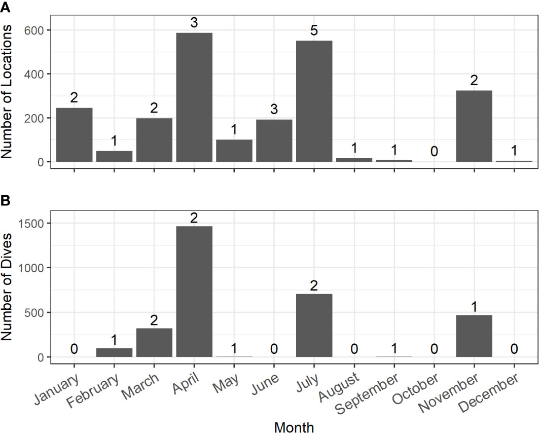
Figure 2 Distribution of filtered locations (A, from 16 tags) and dives (B, from 8 tags) across months from satellite tags deployed on Risso’s dolphins in the Southern California Bight between 2009 – 2019. The number of tags that contribute to monthly data are denoted above each bar.

TABLE 2

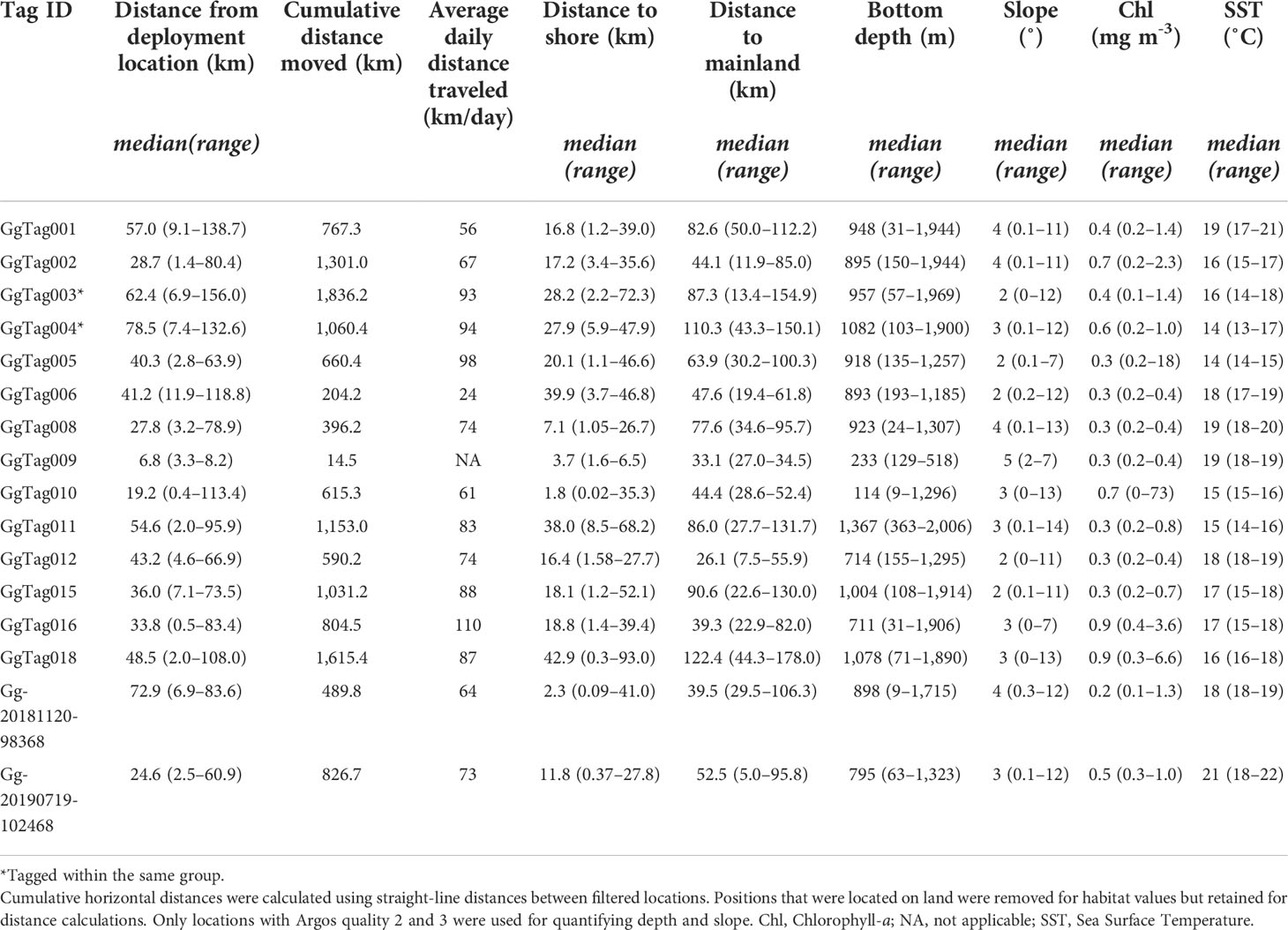
Table 2 Summary of habitat characteristics at filtered Argos locations for individual Risso’s dolphins.

Movements revealed by satellite tracking showed individual variation within the Southern California Bight: some animals ranged broadly throughout the Bight, while others remained more localized (Figure 1). Risso’s utilized most of the Bight with the 50% core use centered around San Clemente and Santa Catalina Islands and the surrounding basins (Figure 3), a pattern likely influenced by tagging location. Tagged dolphins utilized habitat within the boundaries of all four U.S. Navy ranges considered (Figure 1). All tags but one were deployed within either the Southern California Range Complex or Point Mugu Sea Range training areas, and 89% of locations fell within these areas, spanning all 11 months that tags transmitted. Fourteen percent of locations fell within the Southern California Anti-submarine Warfare Range and the Shore Bombardment Areas specifically, and dolphins utilized these areas during seven different months of the year.

FIGURE 3

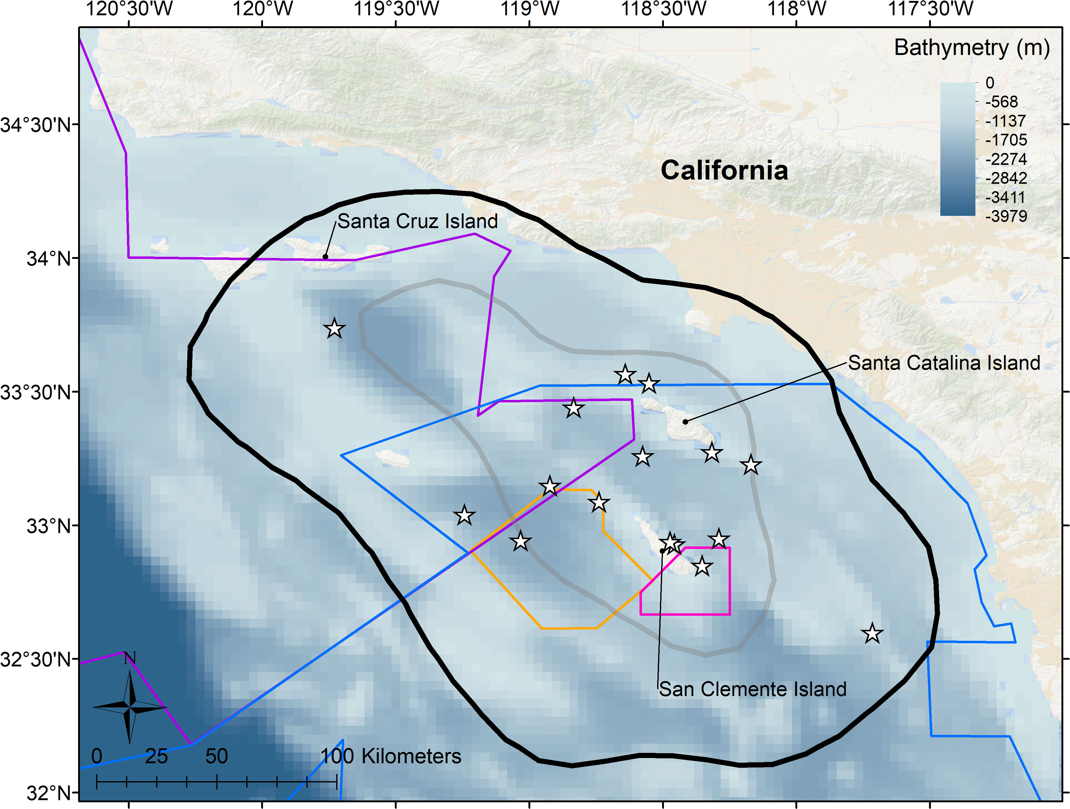
Figure 3 Core use areas for 16 Risso’s dolphins tagged in the Southern California Bight from 2009–2019 as indicated by 50% (gray line) and 95% (black line) kernel density estimates of the combined location data across tags. Stars represent deployment locations. Kernel density isopleths were derived from one average daily position to minimize autocorrelation bias, and are overlayed on high resolution ETOPOv2 bathymetry in meters. Military training ranges are indicated by colored polygons as follows: Blue = Southern California Range Complex; Purple = Point Mugu Sea Range; Orange = Southern California Anti-submarine Warfare Range; Pink = Shore Bombardment Area.

Details of movement model parameter estimation and significance testing are provided in Table 3. Distance from mainland was significantly predicted by time of day, month, and sine of lunar phase (Figures 4A, B, D), while distance from shore was significantly predicted by month and cosine of lunar phase (Figures 4C, E). Animals were found closer to the mainland during first quarter lunar phase and furthest during the last quarter phase (Figure 4D). Animals were predicted to be farther from shore during a full moon compared to during a new moon (Figure 4E), although 95% confidence intervals were large across all lunar phases. Time of day helped explain differences in distance to mainland, although minimally, with animals closer to mainland during the daylight hours versus night (Figure 4A). Seasonality influenced movements with some variability. Animals were generally closer to land (both mainland and shore) in fall and early winter (Figures 4B, C), with closest distances occurring near the islands during that time (Figure 4C).

TABLE 3

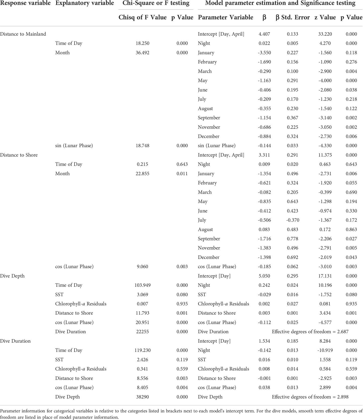
Table 3 Model results including type II Wald chi-square (movement models) or Wald F (dive models) testing and parameter estimation with associated significance testing.

FIGURE 4

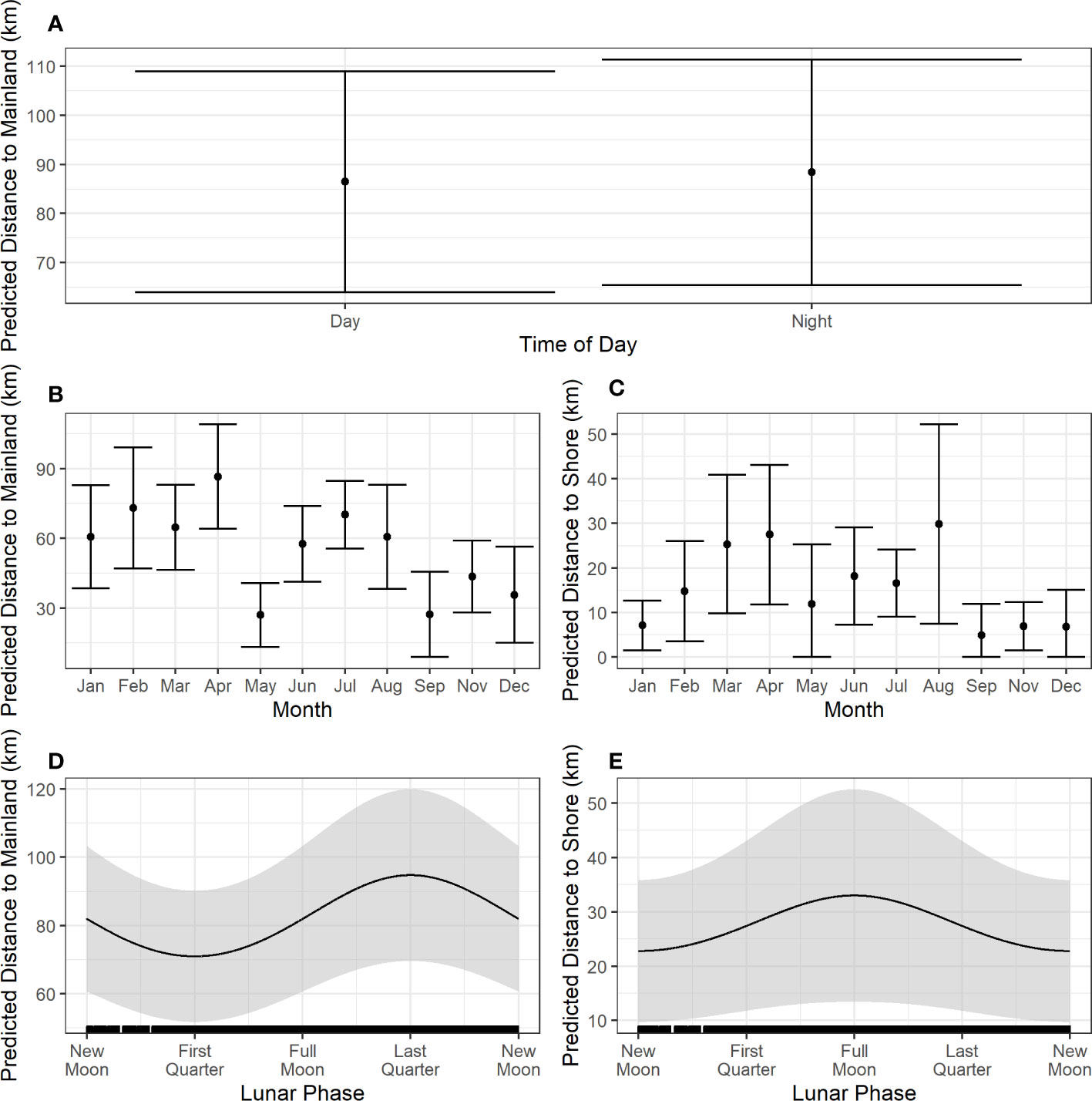
Figure 4 Prediction plots from the fitted models for distance to mainland (A, B, D) and distance to shore (C, E). Solid black lines/dots represent mean predicted values with shaded areas/error bars representing the 95% CI. Hash marks along the x-axis shows the spread of data. For the creation of these plots, values for other predictors in each model were set at the median or modal value as follows: time of day = day, month = April, sine of lunar phase = -0.370, cosine of lunar phase = -0.010.

Dives

A total of 1,469 h of BL data were recorded (n = 8 tags, range = 0.87–428.3 h per tag) (Table 4). Dive data were collected in seven different months across five years from eight of the 16 tagged individuals (Table 1; Figure 2). These data were comprised of 3,071 dives with a grand median (median of all tag medians) depth of 101 m (max = 528 m) and a grand median dive duration of 5.6 min (max = 11.1 min) (Table 4). The maximum dive depth recorded for each dolphin ranged from 148–656 m (Table 4); the longest dive, 16.1 min, was down to 64 m at night. Dives beyond 500 m depth were conducted during both day and night hours, as demonstrated by a sample two-day dive trace (Figure 5A), with comparable frequency (7% of total dives in each period). Animals dove more frequently at night than during the day (p = 8.14e-07), with night and day dive rates at 5.21 (SE = 0.5) and 2.73 (SE = 0.5) dives per hour, respectively. Shallow dives (< 100 m) were more frequent during the day (63%, Figure 5B) versus night (35%, Figure 5B). Across all years and months, Risso’s were documented in median sea surface temperatures of 17˚C (range = 13–22˚C), with the coolest temperatures in June 2010 and warmest in July 2019 (Table 2). The median chlorophyll-a concentration was 0.4 mg m^-3 (range = 0–73) with the lowest and highest concentrations in January 2012 (Table 2).

TABLE 4

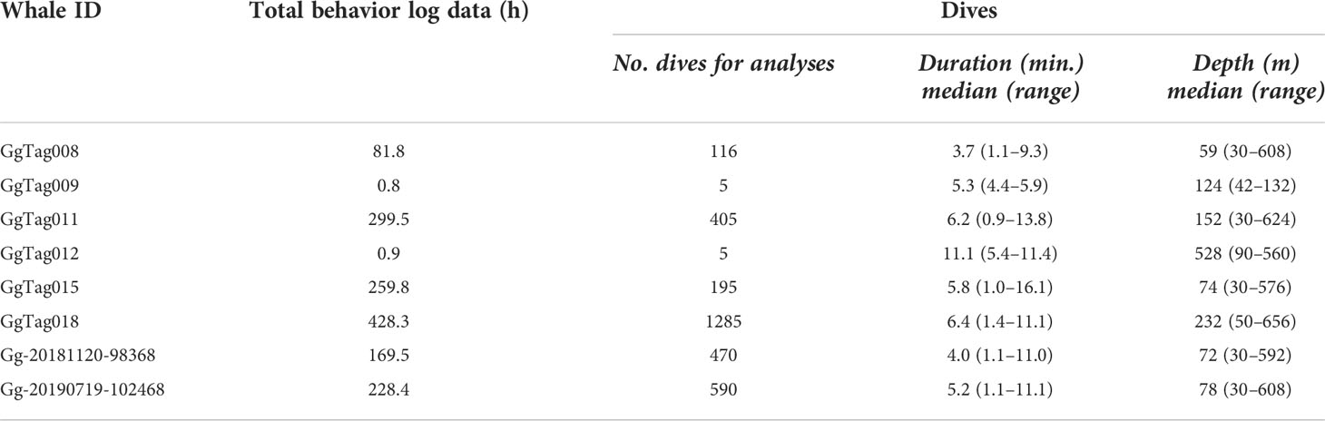
Table 4 Summary of dive parameters by individual of eight Risso’s dolphins satellite-tagged within the Southern California Bight.

FIGURE 5

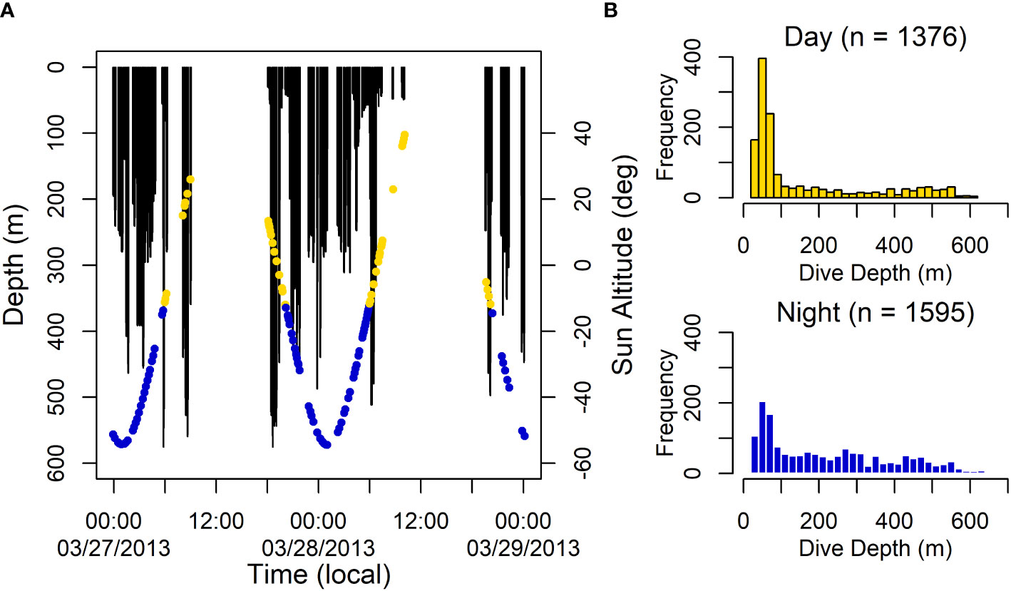
Figure 5 (A) Sample two-day dive trace from a Risso’s dolphin in the Southern California Bight with the time of day denoted by dots for day (yellow) and night (blue). Blanks indicate periods where there are gaps in the data. Extended surface time is indicated by a straight horizontal line along 0 m. (B) Distribution of dive depth estimates for all dive tags during the day and night. For both plots, time of day was defined by a solar altitude (≥ -12 degrees for day and < -12 degrees for night), which was calculated for every dive start at the modeled location estimate closest in time.

Details of dive model parameter estimation and significance testing are provided in Table 3. Dive depth was significantly predicted by dive duration, time of day, distance to shore, and cosine of the lunar phase (Figure 6). Dive duration was significantly predicted by dive depth, time of day, distance to shore, and cosine of lunar phase (Figure 7). Dives were deeper and shorter at night than during the day (Figures 6B, 7B), when dolphins were further offshore (Figures 6C, 7C), and during a full versus a new moon, respectively (Figures 6D, 7D). Wide 95% confidence intervals for dive depth and duration as a function of lunar phase reflect low sample sizes at some lunar phases (see hash marks along x-axis of (Figures 6D, 7D).

FIGURE 6

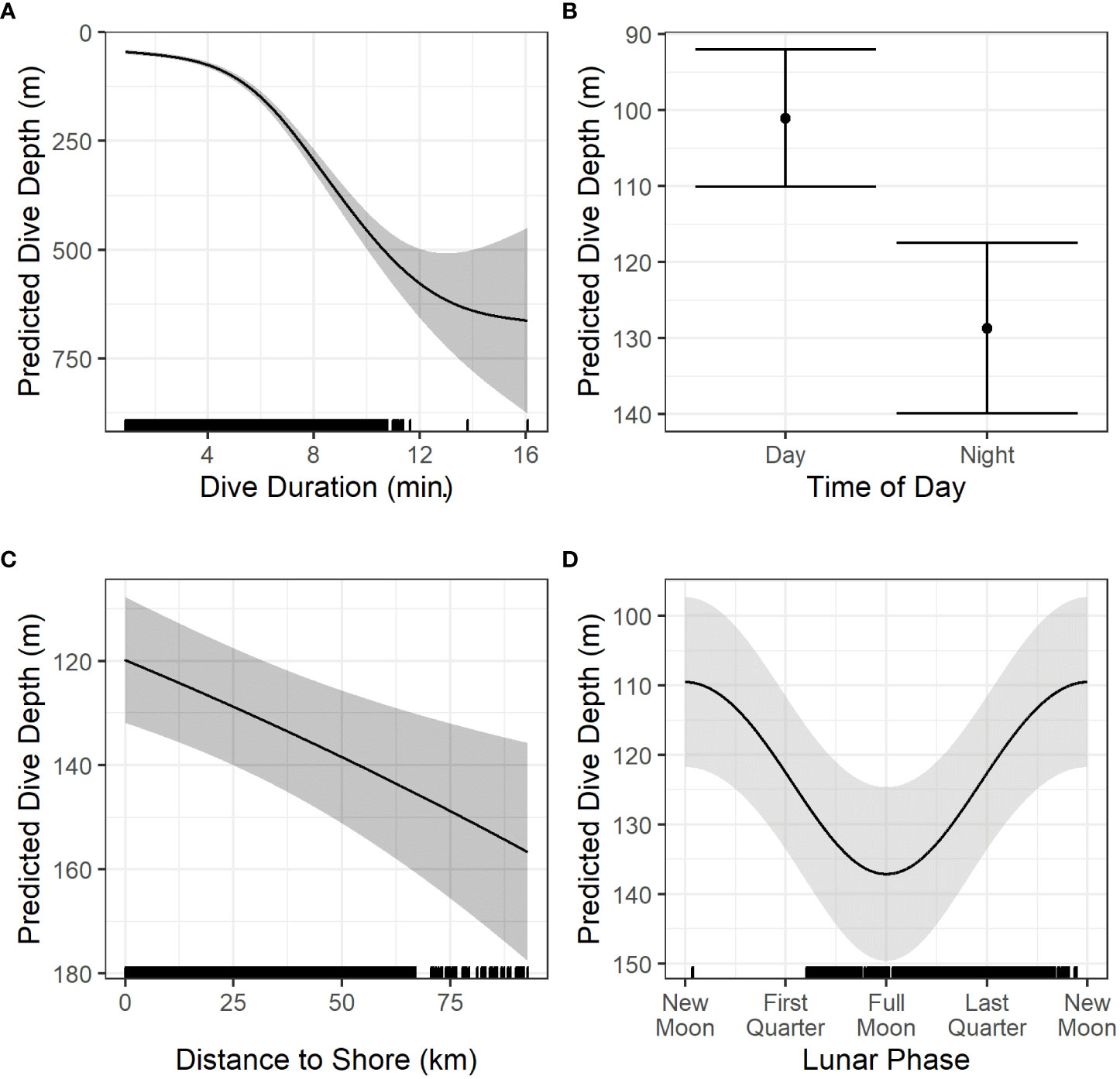
Figure 6 Prediction plots of significant variables (A–D) from the models of dive depth. Solid black lines/dots represent mean predicted values with shaded areas/error bars representing the 95% CI. Hash marks along the x-axis shows the spread of data. For the creation of these plots, values for other predictors in each model were set at the median or modal value as follows: time of day = night, Chl residuals = -0.008, SST = 15.81, distance to shore = 24.68 km, sine of lunar phase = -0.736, cosine of lunar phase = -0.435, dive duration = 5.6 min. Chl, Chlorophyll-a (mg m-3); SST, Sea Surface Temperature (°C).

FIGURE 7

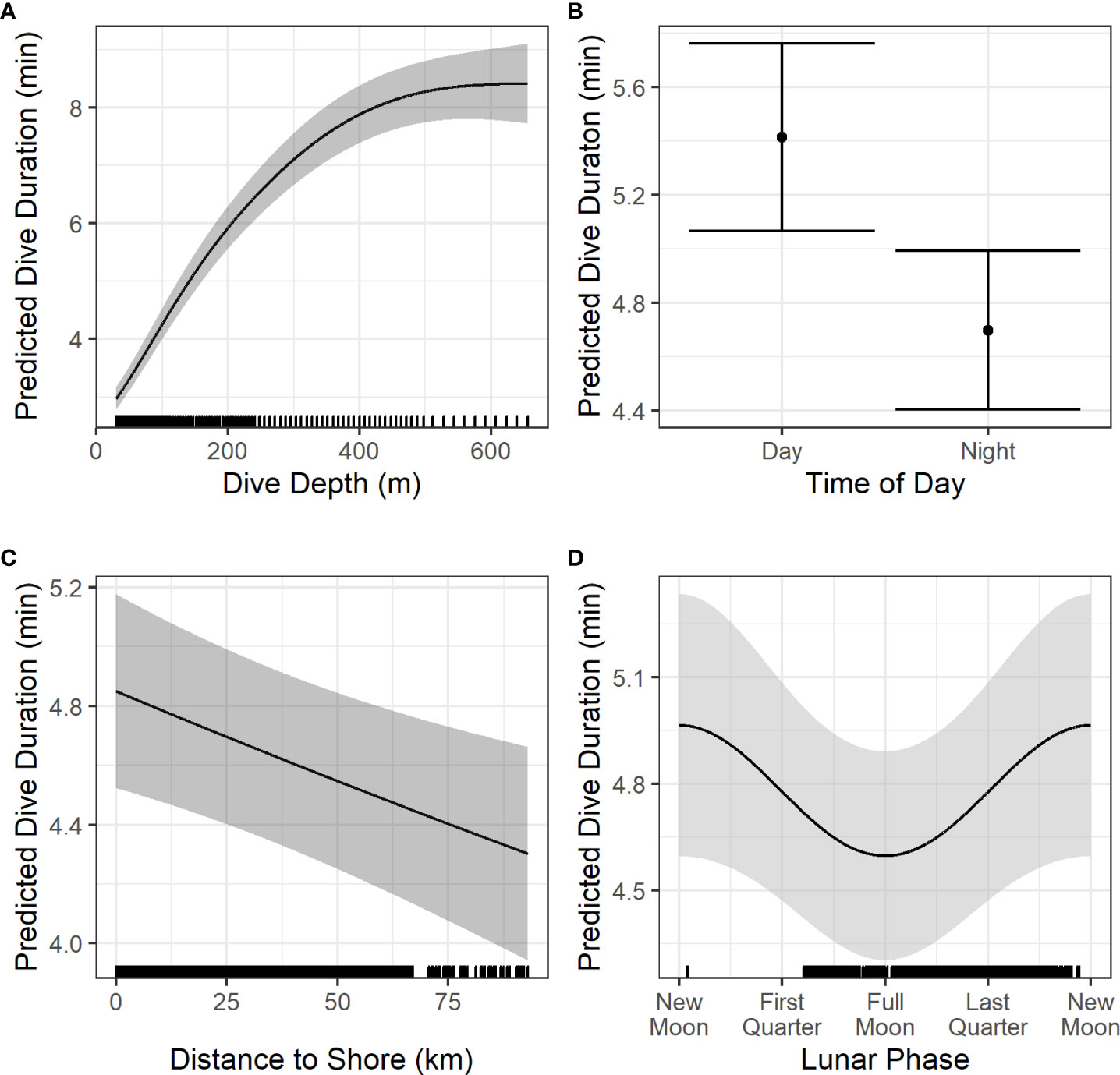
Figure 7 Prediction plots of significant variables (A–D) from the models of dive duration. Solid black lines/dots represent mean predicted values with shaded areas/error bars representing the 95% CI. Hash marks along the x-axis shows the spread of data. For the creation of these plots, values for other predictors in each model were set at the median or modal value as follows: time of day = night, Chl residuals = -0.008, SST = 15.81, distance to shore = 24.68 km, cosine of lunar phase = -0. 435, dive depth = 123.5 m. Chl, Chlorophyll-a (mg m-3); SST, Sea Surface Temperature (°C).

Discussion

As regular inhabitants of the Southern California Bight, Risso’s have been frequently documented on line-transect surveys throughout the region (e.g., Barlow and Forney, 2007; Jefferson et al., 2014a) and across seasons in recent years (e.g., Schorr et al., 2019). Habitat used by tagged dolphins in this study ranged from the deep waters of the numerous basins to the shallow waters inshore of San Clemente and Santa Catalina Islands along the mainland coast (9–2,006 m), with Argos locations sometimes clustered around steep slope features (Figure 1). Globally, densities of Risso’s appear higher over the outer continental shelf and upper regions of the continental slope (Jefferson et al., 2014b). The patchy distribution and local abundance of this species may be driven by enhanced productivity associated with currents and upwellings characteristic of these steep topographic areas (Kruse et al., 1999). Outside of the Southern California Bight, they are documented in various habitats ranging from shallow waters such as 2–5 m in Monterey Bay, CA (Jefferson et al., 2014b) to offshore pelagic waters of Hawai'i in depths exceeding 3,000 m (Baird, 2016). In the Azores around Pico Island, they can be found from 0–10 km from shore (Hartman et al., 2016) where steeply sloped nearshore topography results in water depths increasing from 200 m to 1000 m within 5 km (Hartman et al., 2008).

While relatively short deployment durations of this study preclude any meaningful discussion of large-scale movements into and out of the Southern California Bight, they do provide new insights into localized movements. Changes in Risso’s density indicate latitudinal seasonal shifts occur along the U.S. west coast (Green et al., 1992; Forney and Barlow, 1998). In the Bight, Santa Catalina Island has repeatedly been identified as important habitat for Risso’s (Shane, 1995a; Shane, 1995b; Soldevilla et al., 2010), with acoustic detections occurring on 75% of the days at a site on the south end of the island (Soldevilla et al., 2010). The near year-round acoustic presence at Santa Catalina Island may suggest that an island-associated population exists and/or a greater Southern California Bight resident population, with possible seasonal influx from a larger migratory population (Soldevilla et al., 2010). In this study, all Risso’s were tagged in the outer waters (defined as waters offshore of the mainland coast) of the Southern California Bight, mainly in the greater surrounding waters of the outer Channel Islands. Nearly all individuals spent at least some of their time within the shallower nearshore waters of these islands (Figure 1). Of the 16 Risso’s, 12 approached within 20 km of Santa Catalina Island (Figure 1), in all seasons and in eight different years. Of these 12, only half were tagged within 20 km of this island (min = 3 km). All but one of these six tags also left this island; the brief transmission for the sixth tag prevents further discussion of its movements. In fact, the only animal out of the 16 that demonstrated close association with Santa Catalina Island for most of its tag transmission was actually tagged in the San Nicolas Basin on the west side of San Clemente Island. While these tags may not confirm or refute the presence of island-associated individuals or populations, they do further demonstrate the importance of Santa Catalina Island for the broader, regional population throughout the year.

While animals in this study were tagged in all but one month of the year, all remained within the Southern California Bight despite demonstrating varied and often highly mobile movement patterns, and most remained relatively local to their tagging location (Figure 3), suggesting year-round residence within the Bight is plausible. Alternatively, if some of these individuals were members of the larger Washington-Oregon-California migratory stock, it is entirely feasible that the limited number of tags and their generally short durations simply did not capture movements out of this region. Unfortunately, durations like these are not uncommon for remotely deployed tags on small cetaceans, where factors including surface activity, interactions with conspecifics, and the challenge of achieving optimal tag placement often lead to premature detachments.

The seasonality of inshore/offshore movements were most apparent when considering distance to any landmass, rather than to the mainland coast. According to our models, Risso’s were significantly closer to land, though this was typically an island, from September through January (p < 0.05). Although market squid spawn in the Southern California Bight year-round (Navarro et al., 2018), concentrated spawning aggregations occur nearshore over shallow sandy substrate in southern California along the mainland coast and the Channel Islands (Zeidberg et al., 2012; Van Noord, 2017) from October through April/May (Fields, 1965). Past observational research suggested that both Risso’s and short-finned pilot whales (Globicephala macrorhynchus), another squid-eating species common within the Southern California Bight prior to the 1982–83 El Niño event, shift into the Channel Islands during the winter months to feed on spawning market squid (Sinclair, 1992; Shane, 1995b). Our data suggest this seasonal, prey-driven shift has continued in the decades since. These may be fine-scale, localized shifts by animals that remain within the greater Southern California Bight throughout the year, those of migratory animals shifting into the Bight, or both.

While earlier research in the Bight suggested that Risso’s foraged at night (Shane 1995a; Soldevilla et al., 2010) with slow travel/rest the predominant daytime behaviors (Shane, 1995b; Smultea et al., 2018), more recent studies have documented daytime foraging excursions (Arranz et al., 2018; Arranz et al., 2019; Benoit-Bird et al., 2019). Dives in excess of 500 m recorded on these tags occurred across all times of day (max = 607 m day, 656 m night) (Figure 5B) and are comparable to results from Benoit-Bird et al. (2019). Dives were predicted to be 1.27 times deeper (e^β; β = 0.24, SE = 0.02, p-value < 2e-16) and 4.70 times shorter (e^β; β = -0.14, SE = 0.01, p-value < 2e-16) at night versus day (Figures 6B, 7B), and to occur nearly twice as often. This depth difference is potentially driven by both a greater number of dives at < 100 m depth during the day (63% day versus 35% night) and > 100 m at night (65% night versus 37% day) (Figure 5B). These results would align with increased nighttime foraging activities that have been described previously (Soldevilla et al., 2010; Arranz et al., 2019; Benoit-Bird et al., 2019). While Benoit-Bird et al. (2019) documented elevated Risso’s echolocation in shallow waters at night, we are unable to make further comparisons due to the limited temporal and spatial coverage of acoustic data and the lack of nighttime tag data from that study.

Described as dynamic foragers, Risso’s target different prey layers, switching between shallow water generalist and deep water specialist strategies (Benoit-Bird et al., 2019) and appear to consider optimal energy investments and tradeoffs prior to the next dive (Arranz et al., 2018; Visser et al., 2021). Jumbo squid are at depths > 250 m during the day, travel to near-surface waters at dusk, and then demonstrate highly variable dive behavior until they presumably find a zone to exploit for food (Gilly et al., 2006). In Hawai'i, the mesopelagic layer migrates from the 400–700 m depth during daylight hours to 0–400 m at night, though pilot whales appear to target the deeper 400 m layer at night, potentially in search of higher caloric prey (Owen et al., 2019). In the Azores, Risso’s target two deep scattering layers, a broad one at 500–700 m and a narrow one at 400 m, with both layers performing diel vertical migration (Visser et al., 2021). Off Santa Catalina Island, Risso’s were detected in three layers: a deep static layer at 450 m, a mid-water migrating layer at 100–300 m, and an intermittent shallow layer at 50 m along with scattered patches consisting of fish and squid (Benoit-Bird et al., 2019). It’s possible that Risso’s utilize the photic advantage of daylight to capitalize on the low energetic costs of shallow layer exploitation in between bouts of deep layer explorations (the switching behavior documented in Benoit-Bird et al., 2019) and thereby conserve energy for nighttime hunts that are directed at preferential prey, such as jumbo squid, that while vertically migratory, are not necessarily reaching shallow waters throughout the nighttime hours.

Lunar phase has been linked to changes in zooplankton biomass (Hernández-León et al., 2002) and depth (Boden and Kampa, 1967) and horizontal displacement in the mesopelagic layer in Hawaiʻi (Benoit-Bird et al., 2009). In this study, lunar phase predicted both horizontal and vertical shifts, albeit with large confidence intervals. Risso’s were located 1.45 times further away from shore (including islands) (Figure 4E) during a full moon than a new moon, a pattern similar to that observed in Hawaiian pilot whales (Owen et al., 2019). Lunar phase has been associated with changing use of the water column in Cuvier’s beaked whales (Ziphius cavirostris) (Barlow et al., 2020) and jumbo squid (Gilly et al., 2006), and like the Risso’s tagged in this study, pilot whales (Owen et al., 2019), Galápagos fur seals (Arctocephalus galapagoensis) (Horning and Trillmich, 1999), and bigeye tuna (Thunnus obesus) (Musyl et al., 2003) all appear to use deeper waters during a full moon. Full moon light levels at 100–150 m are equivalent to mid-day light levels at ~500 m (Clarke and Denton, 1962). Deep scattering layer species seek lower light levels to avoid predators, and are thus found at deeper depths during brightly moonlit nights (Boden and Kampa, 1967), increasing use of near-surface waters at night as the moon wanes (Hernández-León et al., 2002). It may be a cost-effective strategy for Risso’s to pursue prey at deeper depths around a full moon—as suggested by our model—when layers may provide additional biomass to target. The question also should be raised whether changes in dive behavior associated with lunar phases are driven by illumination levels themselves, or whether they are the result of an endogenous signal that is associated with the 29.5 day lunar cycle, or a combination of both. It seems plausible that light may have significant biological influence on marine systems with predominantly clear water and skies but in geographic locations where waters are more turbid and skies are obscured by clouds for at least part of the year, as they are in the Southern California Bight (e.g., Rastogi et al., 2016), an endogenous cue may play a more significant role. In (Benoit-Bird et al., 2009), lunar phase accounted for more variability in micronekton migration than surface irradiance, suggesting that lunar effects other than light levels effect these prey, and in turn, the predators that pursue them.

Results from this study suggest seasonal trends in movements, demonstrate year-round presence within the Bight, and further describes lunar and diel influences on behavior. We have presented our statistical findings and suggest biological explanations based on findings in the literature. However, we must acknowledge that statistical significance according to model output should be interpreted with caution from a biological perspective, as these data have limitations. Although several of these tags lasted nearly three weeks, the kernel density analysis was likely biased by deployment location. In addition to sample size limitations, some of these data included gaps from failed transmission and from short tag durations that didn’t span across seasons and lunar phases. The effects of Argos location quality and resolution, and the resulting prediction errors from modeled animal tracks based on Argos data, further limit interpretation of these results. While we filtered Argos locations to reduce error before using them in standardized movement models, predicted locations had standard errors ranging from 0 to 26 km. There were occasional adjustments to tag programming to optimize data collection that may have affected some statistics. When looking at environmental variables such as sea surface temperature and chlorophyll-a, in-situ measurements collected around an animal is the only way to provide accurate, real-time representation of that variable with high resolution, but this was not available for these tags. Remote sensing can capture patterns in these data over a broad spatial region, but cloud cover is an inherent limitation. Although we were able to combine a remote sensing and an in-situ dataset to derive sea surface temperature at modeled locations, we had to create 8-day averaged composites for chlorophyll-a to create gap free composites. This mismatch in resolution between animal location estimates and environmental variables is another potential source of error. It should be noted that remote sensing can underestimate values for chlorophyll-a and sea surface temperature (Gomez et al., 2020; Keates et al., 2020), and absolute values should be interpreted with caution. These aforementioned factors may have influenced the significance of these predictors in the dive models.

We believe one of the greatest values of these analyses are their ability to aid formulation of new hypotheses and research directions. Additional targeted data collection will strengthen model results and allow for more concrete biological interpretations of these findings. Deployments in other regions of the Southern California Bight as well as during specific periods where data gaps currently exist [e.g., gaps in month (Figure 2) and lunar phase (Figure 6)] would provide a more comprehensive regional dataset. The short duration of these tags highlights the need for more tag development to improve attachment while continuing to minimize impact. A regional photo-identification catalog, genetic analyses, and the use of medium-duration, dart attached archival acoustic tags (e.g., Sweeney et al., 2022) along with prey mapping would provide meaningful connections between the existing research within this region. It is our hope that this work will foster purposeful discussions and ideas for future work to manage and protect this species.

Data availability statement

The raw data supporting the conclusions of this article will be made available by the authors, without undue reservation.

Ethics statement

The animal study was reviewed and approved by Cascadia Research Collective Institutional Animal Care and Use Committee.

Author contributions

BR, EF, GS, and SW conducted the fieldwork. BR, GS, and DS conducted the data analysis. All authors contributed to the article and approved the submitted version.

Funding

Funding for fieldwork and tags was provided by the U.S. Navy, Pacific Fleet (N66604-14-C-0145, N66604-18-P-2187) and via the Californian Cooperative Ecosystems Studies Unit (N62473-19-2-0025), the Chief of Naval Operations Environmental Readiness Division (N45) via a grant from the Naval Postgraduate School (Grant No. N000244-10-1-0050) and the Environmental Security Technology Certification Program (N66604-14-C-2438). Additional support was provided by the Office of Naval Research and the Living Marine Resources program.

Acknowledgments

We would like to thank the U.S. Navy, Pacific Fleet, N45, the Environmental Security Technology Certification Program, the Living Marine Resources program, and the Office of Naval Research for support of this research. We thank all participants from the Marine Mammal Monitoring on Navy Ranges program at the Naval Undersea Warfare Center, Jeff Foster for contributions in the field, and the Naval Postgraduate School and Californian Cooperative Ecosystems Studies Unit for contract facilitation. We thank Stacy DeRuiter for assistance with analyses and Chip Johnson, Jessica Chen, and Shannon Coates and three reviewers for their thoughtful comments and suggestions. This study was conducted under U.S. National Marine Fisheries permits No. 540-1811, 16111, 15330, 20605. Tagging was approved by the Cascadia Research Collective Institutional Animal Care and Use Committee.

Conflict of interest

The authors declare that the research was conducted in the absence of any commercial or financial relationships that could be construed as a potential conflict of interest.

Publisher’s note

All claims expressed in this article are solely those of the authors and do not necessarily represent those of their affiliated organizations, or those of the publisher, the editors and the reviewers. Any product that may be evaluated in this article, or claim that may be made by its manufacturer, is not guaranteed or endorsed by the publisher.

References

Andrews R. D., Baird R. W., Calambokidis J., Goertz C. E. C., Gulland F. M. D., Heide-Jørgensen M. P., et al. (2019). Best practice guidelines for cetacean tagging. J. Cetacean Res. Manage, 27–66. doi: 10.47536/jcrm.v20i1.237

CrossRef Full Text | Google Scholar

Arranz P., Benoit-Bird K. J., Friedlaender A. S., Hazen E. L., Goldbogen J. A., Stimpert A. K., et al. (2019). Diving behavior and fine-scale kinematics of free-ranging risso’s dolphins foraging in shallow and deep-water habitats. Front. Ecol. Evol. 7. doi: 10.3389/fevo.2019.00053

CrossRef Full Text | Google Scholar

Arranz P., Benoit-Bird K. J., Southall B. L., Calambokidis J., Friedlaender A. S., Tyack P. (2018). Risso’s dolphins plan foraging dives. J. Exp. Biol. 221, 1–9. doi: 10.1242/jeb.165209

CrossRef Full Text | Google Scholar

Azzellino A., Gaspari S., Airoldi S., Nani B. (2008). Habitat use and preferences of cetaceans along the continental slope and the adjacent pelagic waters in the western ligurian Sea. Deep Sea Res. Part Oceanogr. Res. Pap. 55, 296–323. doi: 10.1016/j.dsr.2007.11.006

CrossRef Full Text | Google Scholar

Bacon C. E., Smultea M. A., Fertl D., Würsig B., Burgess E. A., Hawks-Johnson S. (2017). Mixed-species associations of marine mammals in the southern California bight, with emphasis on Risso’s dolphins (Grampus griseus). Aquat. Mamm. 43, 177–184. doi: 10.1578/AM.43.2.2017.177

CrossRef Full Text | Google Scholar

Baird R. W. (2002). Risso’s dolphin. Encycl. Mar. Mamm. Acad. Press San Diego CA, 1037–1039.

Google Scholar

Baird R. W. (2016). The lives of hawai‘i’s dolphins and whales: Natural History and Conservation (Honolulu, hawai‘i’: University of hawai‘i’ Press).

Google Scholar

Barlow J., Forney K. A. (2007). Abundance and population density of cetaceans in the California Current ecosystem. Fish. Bull. 105, 509–526.

Google Scholar

Barlow J., Schorr G., Falcone E., Moretti D. (2020). Variation in dive behavior of Cuvier’s beaked whales with seafloor depth, time-of-day, and lunar illumination. Mar. Ecol. Prog. Ser. 644, 199–214. doi: 10.3354/meps13350

CrossRef Full Text | Google Scholar

Barton M (2019). R Package version 1.43.17. https://CRAN.R-project.org/package=MuMIn.

Google Scholar

Baumgartner M. E. (1997). The distribution of Risso’s dolphin (Grampus griseus) with respect to the physiography of the northern Gulf of Mexico. Mar. Mammal Sci. 13, 614–638. doi: 10.1111/j.1748-7692.1997.tb00087.x

CrossRef Full Text | Google Scholar

Bearzi G., Reeves R. R., Remonato E., Pierantonio N., Airoldi S. (2011). Risso’s dolphin Grampus griseus in the Mediterranean Sea. Mamm. Biol. - Z. Für Säugetierkd. 76, 385–400. doi: 10.1016/j.mambio.2010.06.003

CrossRef Full Text | Google Scholar

Benoit-Bird K. J., Au W. W. L., Wisdoma D. W. (2009). Nocturnal light and lunar cycle effects on diel migration of micronekton. Limnol. Oceanogr. 54, 1789–1800. doi: 10.4319/lo.2009.54.5.1789

CrossRef Full Text | Google Scholar

Benoit-Bird K. J., Moline M. A., Southall B. L. (2017). Prey in oceanic sound scattering layers organize to get a little help from their friends: Schooling within sound scattering layers. Limnol. Oceanogr. 62, 2788–2798. doi: 10.1002/lno.10606

CrossRef Full Text | Google Scholar

Benoit-Bird K., Southall B., Moline M. (2019). Dynamic foraging by Risso’s dolphins revealed in four dimensions. Mar. Ecol. Prog. Ser. 632, 221–234. doi: 10.3354/meps13157

CrossRef Full Text | Google Scholar

Bivand R., Lewin-Koh N. (2022) Maptools: Tools for handling spatial objects. Available at: https://CRAN.R-project.org/package=maptools.

Google Scholar

Blanco C., Raduán M. Á., Raga J. A. (2006). Diet of Risso’s dolphin (Grampus griseus) in the western Mediterranean Sea. Sci. Mar. 70, 407–411. doi: 10.3989/scimar.2006.70n3407

CrossRef Full Text | Google Scholar

Bloch D. (2012). Life history of Risso’s dolphin (Grampus griseus) (G. cuvier 1812) in the Faroe Islands. Aquat. Mamm. 38, 250–266. doi: 10.1578/AM.38.3.2012.250

CrossRef Full Text | Google Scholar

Boden B. P., Kampa E. M. (1967). The influence of natural light on the vertical migrations of an animal community in the seas. Symp Zool Soc. Lond 19, 15–26.

Google Scholar

Boer M. N., Clark J., Leopold M. F., Simmonds M. P., Reijnders P. J. H. (2013). Photo-identification methods reveal seasonal and long-term site-fidelity of Risso’s dolphins (Grampus griseus) in shallow waters (Cardigan Bay, Wales). Open J. Mar. Sci. 03, 66–75. doi: 10.4236/ojms.2013.32A007

CrossRef Full Text | Google Scholar

Brooks M. E., Kristensen K., van Benthem K. J., Magnusson A., Berg C., Nielsen A., et al. (2017). glmmTMB balances speed and flexibility among packages for zero-inflated generalized linear mixed modeling. R J. 9, 378–400. doi: 10.32614/RJ-2017-066

CrossRef Full Text | Google Scholar

Calenge C. (2006). The package adehabitat for the R software: a tool for the analysis of space and habitat use by animals. Ecol. Model. 197, 516–519. doi: 10.1016/j.ecolmodel.2006.03.017

CrossRef Full Text | Google Scholar

Cañadas A., Sagarminaga R., Garcıa-Tiscar S. (2002). Cetacean distribution related with depth and slope in the Mediterranean waters off southern Spain. Deep Sea Res. Part Oceanogr. Res. Pap. 49, 2053–2073. doi: 10.1016/S0967-0637(02)00123-1

CrossRef Full Text | Google Scholar

Carretta J., Forney K. A, Oleson E. M, Weller D. W., Lang A. R., Baker J., et al. (2020). U.S pacific marine mammal stock assessments: 2019 La Jolla, CA:U.S. Department of Commerce, NOAA Technical Memorandum NMFS-SWFSC-629.

Google Scholar

Clarke M. R. (1996). Cephalopods as prey. III. Cetaceans. Philos. Trans. R. Soc Lond. B Biol. Sci. 351, 1053–1065. doi: 10.1098/rstb.1996.0093

CrossRef Full Text | Google Scholar

Clarke G. W., Denton E. J. (1962). “Light and animal life,” in The Sea. Ed. Hill M. N. (New York, NY: Interscience), 456–468.

Google Scholar

DeBruyn A. M. H., Meeuwig J. J. (2001). Detecting lunar cycles in marine ecology: Periodic regression versus categorical ANOVA. Mar. Ecol. Prog. Ser. 214, 307–310. doi: 10.3354/meps214307

CrossRef Full Text | Google Scholar

Dohl T., Guess R., Duman M., Helm R. (1983). Cetaceans of central and northern californirnia 1980–1983: Status, abundance, and distribution (Pacific OCS Region, Minerals Management Service, U.S. Dept. of the Interior).

Google Scholar

Douglas D. C., Weinzierl R., C Davidson S., Kays R., Wikelski M., Bohrer G. (2012). Moderating Argos location errors in animal tracking data. Methods Ecol. Evol. 3, 999–1007. doi: 10.1111/j.2041-210X.2012.00245.x

CrossRef Full Text | Google Scholar

Environmental Systems Research Institute ESRI (2019). ArcGIS Desktop: Release 10.7.1 (Redlands, CA:Environmental Systems Research Institute).

Google Scholar

Fields W. G. (1965). The structure, development, food relations, reproduction, and life history of the squid Loligo opalescens Berry. Calif. Dep. Fish Game Fish. Bull. 131, 109.

Google Scholar

Forney K. A., Barlow J. (1998). Seasonal patterns in the abundance and distribution of California cetaceans 1991–1992. Mar. Mammal Sci. 14, 460–489. doi: 10.1111/j.1748-7692.1998.tb00737.x

CrossRef Full Text | Google Scholar

Fox J., Weisberg S. (2019). An R Companion to Applied Regression. 3rd ed. (Thousand Oaks, California, USA: Sage).

Google Scholar

Gilly W., Markaida U., Baxter C., Block B., Boustany A., Zeidberg L., et al. (2006). Vertical and horizontal migrations by the jumbo squid Dosidicus gigas revealed by electronic tagging. Mar. Ecol. Prog. Ser. 324, 1–17. doi: 10.3354/meps324001

CrossRef Full Text | Google Scholar

Gomez A. M., McDonald K. C., Shein K., DeVries S., Armstrong R. A., Hernandez W. J., et al. (2020). Comparison of satellite-based sea surface temperature to in situ observations surrounding coral reefs in La Parguera, Puerto Rico. J. Mar. Sci. Eng. 8, 453. doi: 10.3390/jmse8060453

CrossRef Full Text | Google Scholar

Green G., Brueggeman J., Grotefendt R., Bowlby C., Bonnell M., Balcomb ,. K. III (1992). “Cetacean distribution and abundance off Oregon and Washington,” in Oregon and Washington Marine Mammal and Seabird Surveys: Final report (Los Angeles, Calif: Pacific OCS Region, Minerals Management Service, U.S. Dept. of the Interior).

Google Scholar

Hartman K. L., Visser F., Hendriks A. J. E. (2008). Social structure of Risso’s dolphins (Grampus griseus) at the Azores: A stratified community based on highly associated social units. Can. J. Zool. 86, 294–306. doi: 10.1139/Z07-138

CrossRef Full Text | Google Scholar

Hartman K. L., Wittich A., Cai J. J., van der Meulen F. H., Azevedo J. M. N. (2016). Estimating the age of Risso’s dolphins (Grampus griseus) based on skin appearance. J. Mammal. 97 (2), 490–502.

Google Scholar

Heide-Jørgensen M., Dietz R., Laidre K., Richard P. (2002). Autumn movements, home ranges, and winter density of narwhals (Monodon monoceros) tagged in tremblay sound, Baffin island. Polar Biol. 25, 331–341. doi: 10.1007/s00300-001-0347-6

CrossRef Full Text | Google Scholar

Hernández-León S., Almeida C., Yebra L., Arístegui J. (2002). Lunar cycle of zooplankton biomass in subtropical waters: Biogeochemical implications. J. Plankton Res. 24, 935–939. doi: 10.1093/plankt/24.9.935

CrossRef Full Text | Google Scholar

Horning M., Trillmich F. (1999). Lunar cycles in diel prey migrations exert a stronger effect on the diving of juveniles than adult Galápagos fur seals 6. doi: 10.1098/rspb.1999.0753

CrossRef Full Text | Google Scholar

Jeanniard-du-Dot T., Holland K., Schorr G. S., Vo D. (2017). Motes enhance data recovery from satellite-relayed biologgers and can facilitate collaborative research into marine habitat utilisation. Anim. Biotelem. 5, 1–15. doi: 10.1186/s40317-017-0132-0

CrossRef Full Text | Google Scholar

Jefferson T. A., Smultea M. A., Bacon C. E. (2014a). Southern California Bight marine mammal density and abundance from aerial surveys 2008-2013. J. Mar. Anim. Their Ecol. 7, 14–30.

Google Scholar

Jefferson T. A., Webber M. A., Pitman R. L. (2006). Marine Mammals of the World, a Comprehensive Guide to their Identification (Amsterdam: Elsevier).

Google Scholar

Jefferson T. A., Weir C. R., Anderson R. C., Ballance L. T., Kenney R. D., Kiszka J. J. (2014b). Global distribution of Risso’s dolphin Grampus griseus : A review and critical evaluation. Mammal Rev. 44, 56–68. doi: 10.1111/mam.12008

CrossRef Full Text | Google Scholar

Johnson D., London J. (2018). Crawl: An R package for fitting continuous-time correlated random walk models to animal movement data. Available at: https://CRAN.R-project.org/package=crawl.

Google Scholar

Johnson D. S., London J. M., Lea M.-A., Durban J. W. (2008). Continuous-time correlated random walk model for animal telemetry data. Ecology 89, 1208–1215. doi: 10.1890/07-1032.1

PubMed Abstract | CrossRef Full Text | Google Scholar

Kaplan D., Pruim R. (2020). Ggformula: Formula interface to the grammar of graphics. Available at: https://CRAN.R-project.org/package=ggformula.

Google Scholar

Keates T. R., Kudela R. M., Holser R. R., Hückstädt L. A., Simmons S. E., Costa D. P. (2020). Chlorophyll fluorescence as measured in situ by animal-borne instruments in the northeastern Pacific Ocean. J. Mar. Syst. 203, 103265. doi: 10.1016/j.jmarsys.2019.103265

CrossRef Full Text | Google Scholar

Kelley D., Richards C. (2020). Oce: Analysis of oceanographic data. Available at:https://cran.r-project.org/web/packages/oce/.

Google Scholar

Kruse S. L. (1989). Aspects of the biology, ecology, and behavior of Risso’s dolphins (Grampus griseus) off the California coast (Santa Cruz, CA: University of California).

Google Scholar

Kruse S., Caldwell D. K., Caldwell M. C. (1999). “Risso’s dolphin Grampus griseus,” in Handbook of Marine Mammals. Eds. Ridgeway S. H., Harrison R. (San Diego, California, USA: Academic Press), 183–212.

Google Scholar

Leatherwood S., Perrin W. F., Kirby V. L., Hubbs C. L., Dahlheim M. (1980). Distribution and movements of Risso’s dolphin, Grampus griseus, in the eastern North Pacific. Fish. Bull. 77, 951–963.

Google Scholar

Lopez R., Malarde J.-P., Royer F., Gaspar P. (2014). Improving Argos Doppler location using multiple-model kalman filtering. IEEE Trans. Geosci. Remote Sens. 52, 4744–4755. doi: 10.1109/TGRS.2013.2284293

CrossRef Full Text | Google Scholar

Luna A., Sanchez P., Chicote C., Gazo M. (2021). Cephalopods in the diet of Risso’s dolphin (Grampus griseus) from the Mediterranean Sea: A review. Mar. Mammal Sci. 38, 725–741.

Google Scholar

Markaida U., Sosa-Nishizaki O. (2003). Food and feeding habits of jumbo squid Dosidicus gigas (Cephalopoda: Ommastrephidae) from the Gulf of California, Mexico. J. Mar. Biol. Assoc. U. K. 83, 507–522. doi: 10.1017/S0025315403007434h

CrossRef Full Text | Google Scholar

McClintock B. T., London J. M., Cameron M. F., Boveng P. L. (2015). Modelling animal movement using the Argos satellite telemetry location error ellipse. Methods Ecol. Evol. 6, 266–277. doi: 10.1111/2041-210X.12311

CrossRef Full Text | Google Scholar

Mendelssohn (2017) Xtractomatic: Accessing environmental data from ERD’s ERDDAP server. Available at: https://CRAN.R-project.org/package=xtractomatic.

Google Scholar

Milani C. B., Vella A., Vidoris P., Christidis A., Koutrakis E., Frantzis A, et al (2017). Cetacean stranding and diet analyses in the North Aegean Sea (Greece). J. Mar. Biolog. Assoc U.K. 98 (5), 1011–1028.

Google Scholar

Musyl M. K., Brill R. W., Boggs C. H., Curran D. S., Kazama T. K., Seki M. P. (2003). Vertical movements of bigeye tuna (Thunnus obesus) associated with islands, buoys, and seamounts near the main Hawaiian islands from archival tagging data. Fish. Oceanogr. 12, 152–169. doi: 10.1046/j.1365-2419.2003.00229.x

CrossRef Full Text | Google Scholar

National Centers for Environmental Information (2006) Two-minute gridded global relief data (ETOPO2v2). Available at: https://ngdc.noaa.gov/mgg/global/etopo2.html.

Google Scholar

Navarro M. O., Parnell P. E., Levin L. A. (2018). Essential market squid (Doryteuthis opalescens) embryo habitat: A baseline for anticipated ocean climate change. J. Shellfish Res. 37, 601–614. doi: 10.2983/035.037.0313

CrossRef Full Text | Google Scholar

Norris K. S., Prescott J. (1961). Observations on Pacific cetaceans of Californian and Mexican waters. Univ. Calif. Publs. Zool. 63, 291–402.

Google Scholar

Orr R. T. (1966). Risso’s dolphin on the Pacific coast of North America. J. Mammal. 47, 341–343. doi: 10.2307/1378142

CrossRef Full Text | Google Scholar

Owen K., Andrews R., Baird R., Schorr G., Webster D. (2019). Lunar cycles influence the diving behavior and habitat use of short-finned pilot whales around the main Hawaiian islands. Mar. Ecol. Prog. Ser. 629, 193–206. doi: 10.3354/meps13123

CrossRef Full Text | Google Scholar

Pedersen T. L. (2020) Patchwork: The composer of plots. Available at: https://CRAN.R-project.org/package=patchwork.

Google Scholar

Rastogi B., Williams A. P., Fischer D. T., Iacobellis S. F., McEachern K., Carvalho L., et al. (2016). Spatial and temporal patterns of cloud cover and fog inundation in coastal California: Ecological implications. Earth Interact. 20, 1–19. doi: 10.1175/EI-D-15-0033.1

PubMed Abstract | CrossRef Full Text | Google Scholar

R Core Team. (2021). R: A language and environment for statistical computing. R Foundation Stat. computing (Vienna, Austria). Available at: https://www.Rproject.org/

Google Scholar

Reeves R. R., Stewart B. S., Clapham P. J., Powell J. A. (2002). Guide to Marine Mammals of the World (New York: Alfred A. Knopf).

Google Scholar

Reynolds R. W., Smith T. M., Liu C., Chelton D. B., Casey K. S., Schlax M. G. (2007). Daily high-resolution-blended analyses for sea surface temperature. J. Clim. 20, 5473–5496. doi: 10.1175/2007JCLI1824.1

CrossRef Full Text | Google Scholar

Schorr G. S., Falcone E. A., Moretti D. J., Andrews R. D. (2014). First long-term behavioral records from Cuvier’s beaked whales (Ziphius cavirostris) reveal record-breaking dives. PloS One 9, e92633. doi: 10.1371/journal.pone.0092633

PubMed Abstract | CrossRef Full Text | Google Scholar

Schorr G. S., Rone B. K., Falcone E. A., Keene E. L., Sweeney D. A. (2019). Cuvier’s beaked whale and fin whale surveys at the Southern California Anti-submarine Warfare Range (SOAR). Final Report to the 1753, US Navy Pacific Fleet Integrated Comprehensive Monitoring Program, 54.

Google Scholar

Shane S. H. (1995a). Behavior patterns of pilot whales and Risso’s dolphins off Santa Catalina Island, California. Aquat. Mamm. 21, 195–197.

Google Scholar

Shane S. H. (1995b). Relationship between pilot whales and Risso’s dolphins at Santa Catalina Island, California, USA. Mar. Ecol. Prog. Ser. 123, 5–11. doi: 10.3354/meps123005

CrossRef Full Text | Google Scholar

Sinclair E. H. (1992). Stomach contents of four short-finned pilot whales (Globicephala macroryhnchus) from the Southern California Bight. Mar. Mammal Sci. 8, 76–81. doi: 10.1111/j.1748-7692.1992.tb00127.x

CrossRef Full Text | Google Scholar

Smultea M. A., Lomac-MacNair K., Nations C. S., McDonald T., Würsig B. (2018). Behavior of Risso’s dolphins (Grampus griseus) in the Southern California Bight: An Aerial Perspective. Aquat. Mamm. 44, 653–667. doi: 10.1578/AM.44.6.2018.653

CrossRef Full Text | Google Scholar

Soldevilla M. S., Wiggins S. M., Hildebrand J. A. (2010). Spatial and temporal patterns of Risso’s dolphin echolocation in the Southern California Bight. J. Acoust. Soc Am. 127, 124–132. doi: 10.1121/1.3257586

PubMed Abstract | CrossRef Full Text | Google Scholar

Soldevilla M. S., Wiggins S. M., Hildebrand J. A., Oleson E. M., Ferguson M. C. (2011). Risso’s and Pacific white-sided dolphin habitat modeling from passive acoustic monitoring. Mar. Ecol. Prog. Ser. 423, 247–260. doi: 10.3354/meps08927

CrossRef Full Text | Google Scholar

Sweeney D. A., Schorr G. S., Falcone E. A., Rone B. K., Andrews R. D., Coates S. N., et al. (2022). Cuvier’s beaked whale foraging dives identified via machine learning using depth and triaxial acceleration. Mar. Ecol. Prog. Ser. 692, 195–208. doi: 10.3354/meps14068

CrossRef Full Text | Google Scholar

Van Noord J. E. (2017). Dynamic spawning patterns in the California market squid (Doryteuthis opalescens) inferred through paralarval observation in the Southern California Bight–2019. Mar. Ecol. 41 (4), e12598.

Google Scholar

Visser F., Keller O. A., Oudejans M. G., Nowacek D. P., Kok A. C. M., Huisman J., et al. (2021). Risso’s dolphins perform spin dives to target deep-dwelling prey. R. Soc. Open Sci. 8, 202320. doi: 10.1098/rsos.202320

PubMed Abstract | CrossRef Full Text | Google Scholar

Watanabe H., Kubodera T., Moku M., Kawaguchi K. (2006). Diel vertical migration of squid in the warm core ring and cold water masses in the transition region of the western North Pacific. Mar. Ecol. Prog. Ser. 315, 187–197. doi: 10.3354/meps315187

CrossRef Full Text | Google Scholar

Wickham H. (2016). ggplot2: Elegant graphics for data analysis (New York: Springer-Verlag).

Google Scholar

Wood S. N. (2011). Fast stable restricted maximum likelihood and marginal likelihood estimation of semiparametric generalized linear models. J. R. Stat. Soc Ser. B Stat. Methodol. 73, 3–36. doi: 10.1111/j.1467-9868.2010.00749.x

CrossRef Full Text | Google Scholar

Wood S., Scheipl F. (2020). gamm4: Generalized Additive Mixed Models using “mgcv” and “lme4”. Available at: https://CRAN.R-project.org/package=gamm4.

Google Scholar

Yates O., Palavecino-Sepúlveda P. (2011). On the stomach contents of a Risso’s dolphin (Grampus griseus) from Chile, southeast Pacific. Lat. Am. J. Aquat. Mamm. 9, 171–173. doi: 10.5597/lajam00185

CrossRef Full Text | Google Scholar

Zeidberg L. D., Butler J. L., Ramon D., Cossio A., Stierhoff K. L., Henry A. (2012). Estimation of spawning habitats of market squid (Doryteuthis opalescens) from field surveys of eggs off central and southern California. Mar. Ecol. 33, 326–336.

Google Scholar