Long-Term Monitoring of In-Water Abundance of Juvenile Pelagic Loggerhead Sea Turtles (Caretta caretta): Population Trends in Relation to North Atlantic Oscillation and Nesting

1 Introduction

Marine megavertebrates are a vulnerable and threatened group of organisms (Peltier and Ridoux, 2015). Widely migrating megavertebrates deserve special attention  (Furey et al., 2018) because of their longevity, the inaccessibility and international character of their habitat. This makes it more difficult to take coordinated protective actions  (Lascelles et al., 2014). Understanding their demographics is essential for the population assessments and the implementation of protective actions. Reliable long-term indicators of their abundances are needed, measured throughout their distributional and habitat range, allowing to assess the possible causes that may affect such abundances.

Sea turtles have complex life histories that involve ontogenetic habitat shifts and large scale migrations  (Hays and Scott, 2013), the usage of terrestrial, coastal and oceanic habitats and the passage through territorial waters of different countries. All species are classified as endangered. After emerging from their terrestrial nests, loggerhead sea turtles (Caretta caretta) typically move offshore as juvenile oceanic foragers and then shift to more coastal habitats as they mature  (Bolten, 2003a; Bolten, 2003b). They are found in all tropical and temperate seas worldwide with 10 subpopulations recognized by the IUCN  (Wallace et al., 2010; Wallace et al., 2011; Casale and Tucker, 2017). The North Eastern (NE) Atlantic where Madeira Island is situated is used exclusively by what is called the juvenile developmental oceanic life stage  (Dellinger, 1998; Bolten, 2003a; Saavedra et al., 2018). Around Madeira at least 3 different subpopulations are found: Western Atlantic (45%), Cape Verde (5%) and mixed origins (48%) that may include Mediterranean turtles  (Monzón-Argüello et al., 2009; Pipa et al., 2019). These proportions may vary seasonally in Madeiran waters  (Freitas et al., 2018).

Sea turtle population assessments are based on numbers of nesting females and their nests  (National Research Council, 2010; Casale and Tucker, 2017). Other life stages are used to estimate partial mortalities, though important knowledge gaps exist regarding the recruitment to the oceanic stage and the mortality during this stage. Although sea turtles can be monitored by in-water and remote sensing studies  (Kobayashi et al., 2008), most of these studies do not address long-term population abundances.

Juvenile mortality is thought to be high for small juveniles that recruit into the oceanic stage  (Bjorndal et al., 2003b; Sasso and Epperly, 2007; Salmon and Scholl, 2014) but rather low for animals during this life stage  (Bjorndal et al., 2003b). Survival during the oceanic stage is deemed critical for population maintenance and growth  (Crouse et al., 1987), however the oceanic stage is the least known and understood  (Bolten, 2003b). Previous studies in Madeira Island indicated that turtles remain in this stage on average for 7 years  (Bjorndal et al., 2003a). Individuals are thought to make the transition from the pelagic to the neritic life-stage at a minimum of 40 cm curved-carapace-length (CCL)  (Witherington et al., 2006) which would correspond to an estimated age of around 6 years  (Bjorndal et al., 2003a), although having the variable size and age  (McClellan and Read, 2007; Casale et al., 2008; Avens et al., 2013). Since the mean age at sexual maturity for the Western Atlantic sub-population was estimated as 36 – 42 years  (Avens et al., 2015), any variation in abundance during the oceanic stage will strongly affect the recruitment into the following life stages. Ideally, demographic parameters should be monitored across all life stages, but most importantly for the oceanic stage, as this would allow for a timely identification of potential threats.  (Turtle Expert Working Group, 2009; Bjorndal et al., 2011).

Study objective. Obtaining data for spatio-temporal distribution during oceanic stage remains notoriously challenging  (Carr, 1987; Putman et al., 2020). Oceanic stage turtles distribute widely on a basin-wide scale  (Bolten et al., 1998; Dellinger, 1998; McCarthy et al., 2010; Putman et al., 2020). Reasons for local abundance changes can be due to spatial shifts or actual abundance changes. To address these questions we monitored loggerhead turtles on a single location within their distribution range for the period of 15 years. We used these data to test various variables that could influence both abundance as well as spatial shifts. Madeira Archipelago is situated within the NE Atlantic oceanic developmental area that includes the Azores, Madeira and the Canary Islands. We used the growing local touristic whale watching activities  (IFAW, 2009; Sequeira et al., 2009; Krasovskaya, 2018; Radeta et al., 2018; Nunes et al., 2020) as platforms of opportunity to monitor the pelagic loggerhead sea turtles since year 2007 for the period of 15 years. Using spectral analysis we found climatic factors that correlate with abundance variations and indicate area shifts of turtle distribution, while the correlation with nesting data hint at abundance variations. These results contribute to a better understanding of the oceanic stage ecology, highlight the importance of hemisphere-wide influences on ocean life, and point to cost-effective methods capable of monitoring widely dispersed low-density species such as sea turtles.

2 Methods

2.1 Study Location

The study was carried out in Madeira Island, Portugal (32°45’N, 17°00’W) located in the NE deep Atlantic Ocean. Since the conditions on the leeward marine area south of Madeira Island are more protected and warmer  (Caldeira et al., 2002; Caldeira and Sangra, 2012; Alves et al., 2020), large traction of touristic activities focus on these areas  (Sambolino et al., 2022). The insular platform of Madeira is rather steep  (Geldmacher et al., 2000), such that whale-watching activities are mostly conducted over deep water and trenches reaching depths of up to 2000 m. Waters are oligotrophic with some localized small-scale upwelling cells at the island’s flanks. They also include enriched mesoscale eddies of oceanic origin that interact with the islands  (Caldeira, 2019; Narciso et al., 2019). Turtles mostly use the calmer and warmer southern waters to bask at the surface and are thus more easily spotted  (Dellinger et al., 1997; Dellinger, 1998).

2.2 In-Water Monitoring

The crews from commercial whale watching boats were asked to record sea turtle sightings (STS) during each of their trips, primarily conducted once daily. Observers were instructed verbally by the authors of the study, while given a small booklet with all relevant information including a sea turtle identification key and the observation forms. Emphasis was placed on the request to record every trip, even if no turtles were seen.

In a separate dataset of the Madeira Turtle Project (MTP 1994-ongoing), turtles are sampled regularly by trained researchers (using methods as those described in Dellinger et al. (1997) and Delgado et al. (2010), where the frequencies of other species except loggerheads are negligible (99.83% of 1800 sightings and captures). Thus all turtle sightings were considered loggerheads, and the boat crew abilities were not rigorously validated as in other studies  (Houghton et al., 2003). For instance, Leatherback-turtles (Dermochelys coriacea), Hawksbills (Eretmochelys coriacea) and Kemp’s Ridleys (Lepidochelys kempii) are easily distinguished as different, however their frequencies, as recorded by an experienced researcher (TD), are in Madeira Island below 0.06%. Conversely, Greens (Chelonia mydas) are rare (~ 5 residents), only appeared regularly at Madeira since 2018, tend to stay close to the shore, and thus do not frequent the same areas as the boats. Most crew members were very experienced local seafarers and would register any turtle as different if they spotted it, since the observation form included specific areas for “other species”.

We used 3 different whale watching companies, two based at Funchal marina (32°38.7’N, 16°54.6’W), and one at Calheta marina (32°43.1’N, 17°10.3’W) further westward (Figure 1). On average, single trip duration was generally between 2.5 - 3 hours. Crews consisted of 2 - 3 persons, with the one completing the observation forms typically being a marine biologist. Used sea vessels varied and included: rigid inflatable boats (RIB 9m), a wooden former fishing boat (12m), and large catamarans (20 – 24m). The distributed observation forms were printed on paper and were kept succinct, not to overload crew-members with data registration. Crew members performing the data entries were asked to write down the number of sighted turtles during the trip. Additional data registered included weather, the Beaufort scale (0-12, byWorld Meterological Organization, 2012), including the estimates of maximum distance to shore and average distance to the shore during the trip, but were not used in this study. Furthermore, crews were asked to record other important species for turtles such as jellyfish (as food species). In the remainder of the paper, to all of the observed loggerhead turtles by the boat crew, we will refer to as sea-turtle sightings (STS).

FIGURE 1

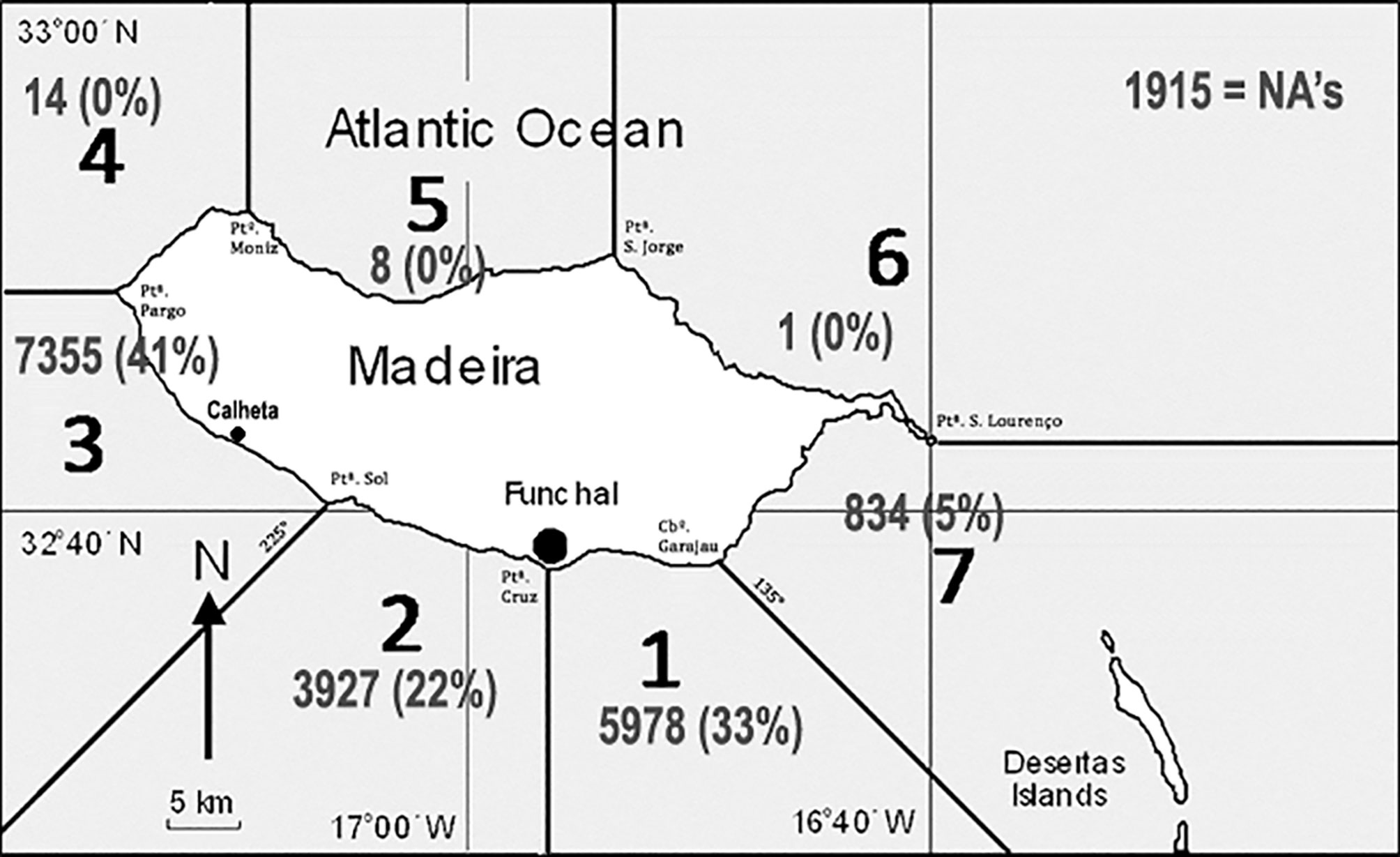
Figure 1 Map of Madeira Island showing the divisions into counting sectors as well as the locations of the marinas of Funchal and Calheta. The numbers represent sampling effort in each sector as number of trips and percent of all trips (NA indicates trips with no recorded sector).

The observation form was improved through time. Until 2009, we solely recorded trip starting time since the average duration of whale-watching trips had a little variation. In 2009, we started recording return times and were thus able to compute the actual time-at-sea for each trip. We furthermore subdivided the island into 7 radial sectors based on conspicuous shoreline features (Figure 1). All crews were asked to register their visited sectors during each single trip. Starting in 2011, the observers were asked to record the data based on times spent in each sector for each trip. The last version was integrated into the local law on marine vertebrate observation  (Regional da Madeira, 2013). In summary, turtle abundance is available in the collected database as “sightings per trip” (complete set), “sightings per hour at sea” (available since 2009), or “sightings per hour and sector” (available since 2011). Though all sectors were sampled, sampling of sectors 4 - 6 was negligible, as most sampling occurred in sectors 1 - 3 and to a lesser extent in sector 7.

2.3 Data Pre-Processing

We use the spectral decomposition by wavelets  (Torrence and Compo, 1998) and Fast Fourier Transform  (Brigham and Morrow, 1967) – WT and FFT, as well as DSP techniques to isolate, analyze, and correlate the most dominant periods in the time series of observed STS against Hurrell North Atlantic Oscillation (NAO) index  (Hurrell and Deser, 2010) and Florida Index Nesting Beach Survey of loggerhead sea turtles nesting (NEST) by the Fish and Wildlife Research Institute’s (FWRI). All three signals (Figure 2) were matched to the same period of the complete STS set (from 2007 - 01 to 2021 - 07).

FIGURE 2

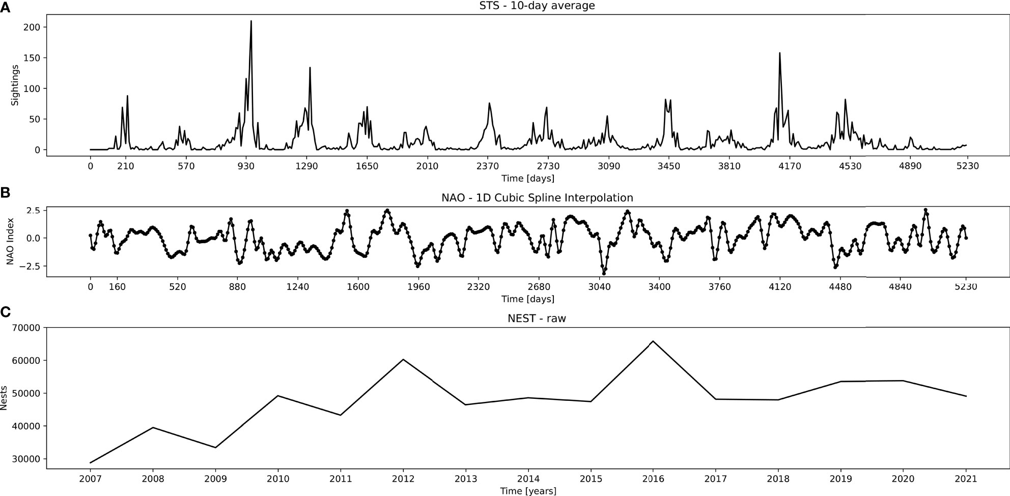
Figure 2 Used datasets, top to bottom: (A) STS – 10-day average points of sea turtle sightings, (B) NAO – interpolated NAO index average air pressure, and (C) NEST – yearly nesting of loggerhead sea turtles in peninsular Florida. Abscissa depicts points matching the sampled STS period (from 2007 - 01 to 2021 - 07).

STS Dataset. During 15 years of sampling, a total of 20032 records were obtained, representing 5300 days. Out of these, 1554 days had no surveying trips, 691 days had only a single record, while all remainder days had more than 1 record up to 28 records per day. Raw data were summarized by month and 10-day blocks by adding all turtles sighted in the period. The last block of a month can vary between 8-11 days. A maximum of 523 data points (i.e. 5230 days, Figure 2A) were formed. STS further contained 15 missing records which were linearly interpolated from nearby points.

NAO Dataset. NAO signal was obtained from its online repository.¹ Since the NAO signal points were given as a monthly average, we boosted the signal time resolution by applying a cubic spline interpolation on in-between points (Figure 2B). This way we introduced 10-day average points after each succeeding monthly point, thus matching the STS time series format. Due to this, in the analysis of NAO signal we neglected any time periods shorter than the original time resolution of 1 month.

NEST Dataset. This dataset was also obtained from its online repository². The default NEST contained the number of loggerhead turtle nests counted on core index beaches in peninsular Florida. The signal contained yearly plots with sampling during a 109-day time window (May 15 through August 31). Since the dataset is given solely as an image, we used R software to extract the data points from the obtained graph (Figure 2C).

2.4 STL Decomposition

We perform an initial signal decomposition using STL  (Cleveland et al., 1990), pointing to the limitations of its use in the present case. For the initial data transformations and STL decomposition we used “R”  (R Development Core Team, 2021) as well as various packages, i.e.: dplyr  (Wickham et al., 2022), reshape  (Wickham, 2007), TSA (Chan and Ripley, 2020), car (Fox and Weisberg, 2019). To avoid problems arising from the present zeros, a value of 1 was added to each value of the time series  (Cowpertweit and Metcalfe, 2009). Seasonal decomposition and trend extraction was done using STL  (Cleveland et al., 1990), a locally weighted loess regression technique  (Cowpertweit and Metcalfe, 2009).

2.5 Spectral Analysis

Since STL decomposition is limited, we propose a method of using DSP in signal decomposition. The spectral analysis is conducted on STS, NAO and NEST datasets, including the cross-correlations between them. At first we analyze all signals time series by isolating the most dominant signal periods using DSP. We inspect how they are related to each other, to distinguish whether individually observed periods correspond to higher harmonics of fundamental modes, or whether they appear as independent oscillations in the time series. For that purpose we use Wavelet Transform (WT) allowing us to recognize patterns of most dominant periods, and time intervals of their appearance in the signal. By applying digital filters (high-, low-, and band- pass respectively, hereinafter abbreviated as HP, LP and BP), as well as smoothing average, we isolate characteristic periods from the signal, presented in following section.

3 Results

3.1 STL Decomposition

The turtle abundance (STS) has a strong seasonal pattern showing peaks during the summer months. By using STL decomposition on the span of 36 annual 10 day blocks for the loess window for seasonal extraction, the time series was divided into seasonal, trend and remaining components (see Supplementary Figure 1 in Supplemental Data). To ensure that the sampling effort did not influence our STS signal the same analysis was performed using only boat effort measured as hours-at-sea (Figure 3, left plot). The population trend and boat effort are uncorrelated, thus effectively showing a consistent relative population abundance index for oceanic loggerhead turtles off Madeira. Since STL provides solely seasonal components (Supplementary Figure 1), it cannot be sensitive to other important modes in the signal which can be modulated. Moreover, STL analysis of STS seasonal mode $\left(T_s^{STS}\right)$ provides a monotonic and repetitive signal which is caused by the digital filtering from the libraries that were used. Such signals are typically not found in natural processes, thus we propose the usage of a detailed spectral analysis using the wavelet and Fast Fourier Transforms in combination with DSP techniques.

FIGURE 3

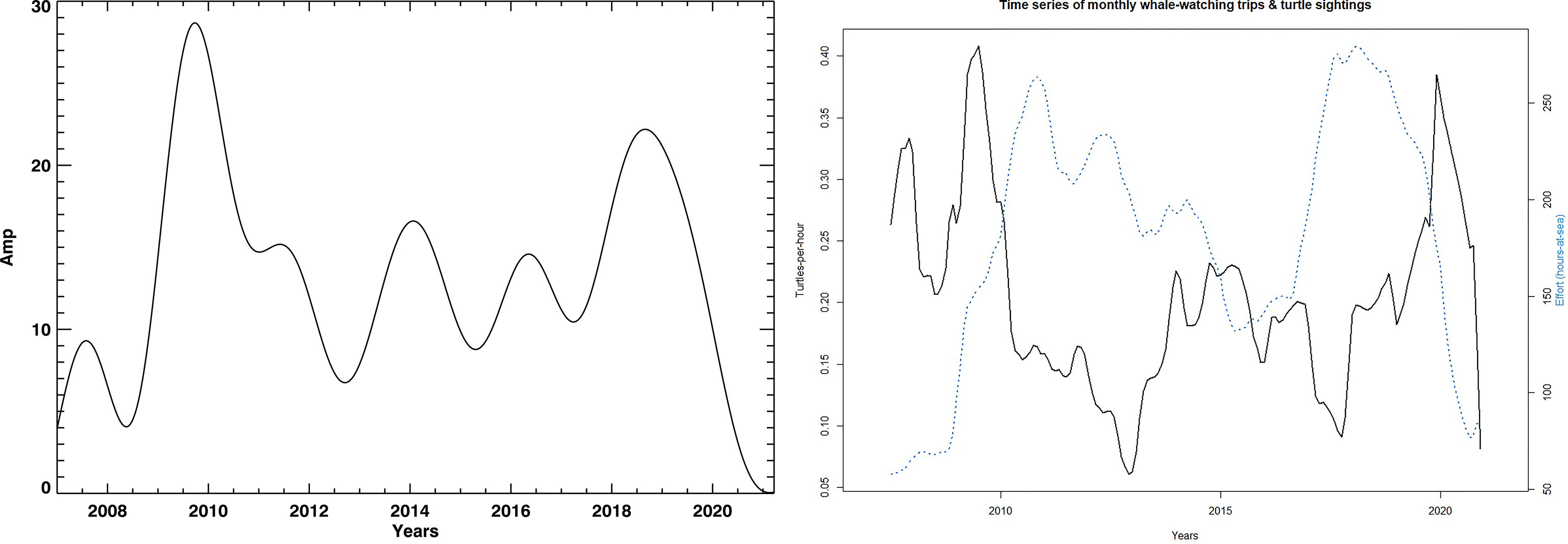
Figure 3 The left plot shows STL decomposition trend lines and boating search effort measured as hour-at-sea (blue) and turtle sightings (black). The right plot shows the trend extracted by using the spectral analysis. It shows a long-period variation in the number of turtle sightings. All trends are shown for the whole interval: 01.01.2007. — 01.07.2021.

3.2 Spectral Analysis

STS Signal Components. The wavelet spectra of the STS signal is shown in Figure 4. It is possible to notice the strong seasonal component which appears as an oscillation with the fundamental period of T_s ~ 365 days, and represents the most dominant component in the signal. This component however includes also the higher harmonic groups around T_s / 2, T_s / 3, and T_s / 4 modes. These higher harmonics are added to the fundamental mode in a way that keeps the integrity of the whole seasonal component. It means that the seasonal component is thus presented (see Supplementary Figure 2 in Supplemental Data) by a periodic change over one year (the fundamental mode) which has a peaked rather than sine-like shape (due to the distortion induced by its higher harmonics). In Supplementary Figure 2, we also show a strong monthly variation (with T_m ~ 30 days) that we isolated from the signal (by HP filtering with T_cut ~ 50 days).

FIGURE 4

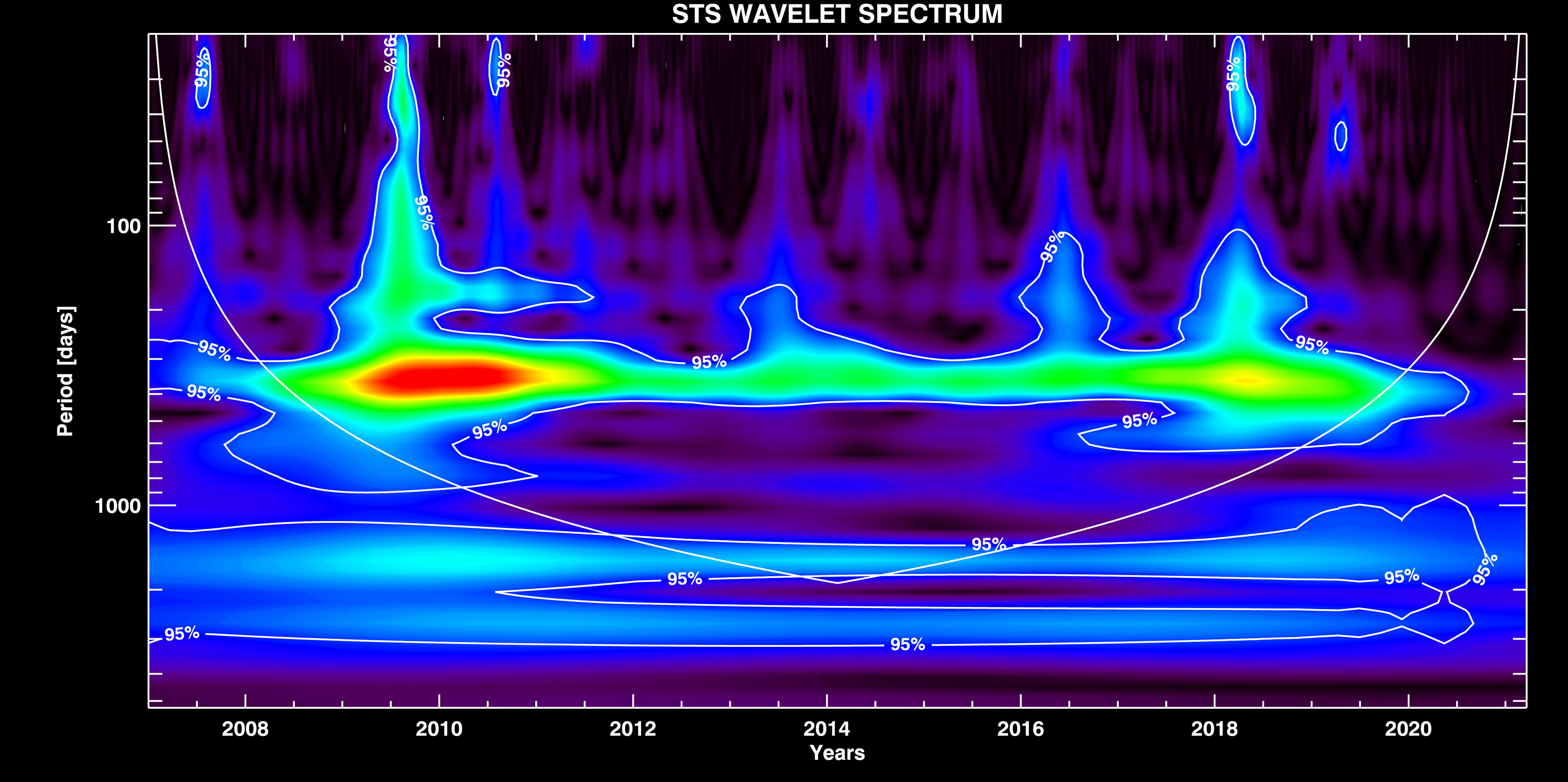
Figure 4 WT of the STS signal with overplotted contours of the significance interval of 0.95 %, and the confidence interval (COI) curve.

As expected, the seasonal component is amplitude modulated (AM) by longer period components which constitute a general long-periodic trend (see Figure 3, right). This trend naturally emerges here as a long period band which is actually the part of the amplitude modulated seasonal component.³ In Supplementary Figure 4, we show the result of cross-correlation between the envelope of the STS seasonal component amplitude change that we get after the demodulation of T_s mode, and, the STS long-period trend. High correlation coefficient (R ~ 0.94) and negligible (relative to T_cut) differential phase shift⁴ imply that the long-period trend is the modulating signal, and T_s mode is the carrier signal in this case. It means that the original long period trend (the low-frequency band of the envelope) can be simply extracted from the signal by using the LP filtering. The advantage of using the spectral analysis over STL resides in the fact that the STL technique is used to extract the constant amplitude seasonal component, thus pronouncing the remaining long period part as a trend. This however induces the appearance of artificial shorter period components in the trend (as seen in Figure 3, left), for which, the spectral analysis is immune. In Supplementary Figure 3, we show the trend decomposition to the individual wave modes. One of the trend components has the period T_nino ~ 1700 days ~ 4.7 years which is likely to be caused by El Niño cycle (Trenberth, 1997). It is the same component that we also found in the NAO signal (presented in the following section). Beside the possible El Niño mode, the long-period trend is also composed of one extra long T_long ~ 2600 days ~ 7 years, and one mid-period T_mid ~850 days period components. Although, the largest period component together with the constant background falls out of the confidence interval (COI) curve (Figure 4), it can still be isolated from the trend by applying the LP filter (bottom plot in Supplementary Figure 3). Its presence in the signal may be attributed to some long scale climate change which is unknown to us at the present moment. The mode with T_mid, though looking like being a first harmonic of T_nino, actually appears as superimposed over it.⁵ Therefore, we argue that T_mid component could possibly be related to some shorter period climate variation such as La Niña, or to some other nature factor.⁶

NAO Signal Components. The WT of NAO signal is depicted in Figure 5. As in the STS case, here we also notice the strong seasonal variation T_s ~ 365 days, and the mid-period component T_mid ~ 850 days that is similar to the STS one. Both components are amplitude modulated (AM). The interesting property which shows up in the NAO case is that the modes T_nino and T_long actually modulate the T_s and T_mid components, respectively. The presence of El Niño and extra-long period climate variations in the NAO signal we therefore find by demodulating the seasonal and mid-range components, since the former do not appear directly as independent components in the NAO signal.

FIGURE 5

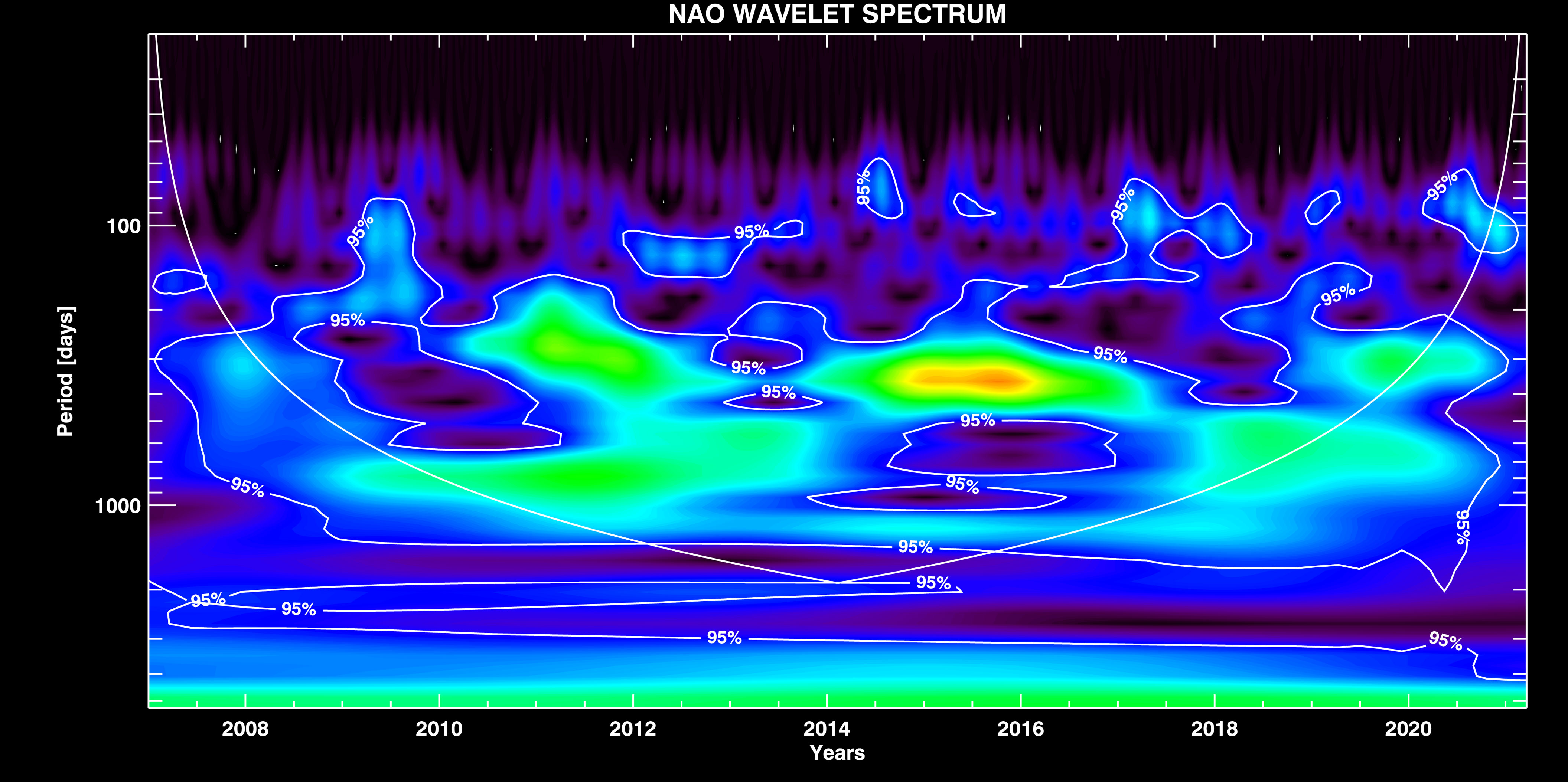
Figure 5 WT of the NAO signal with overplotted contours of the significance interval of 0.95 %, and the confidence interval (COI) curve.

The isolated seasonal and mid-period components are shown in Supplementary Figure 5, together with their envelopes (the periods T_nino and T_long, respectively) which are extracted by demodulation. It is interesting to note that T_long mode modulates T_mid component which, together with T_nino mode, both modulate the amplitude of the seasonal component, resulting in the wavelet spectra observed in Figure 5.

3.3 Signal Correlations

To find relations between the climate component (NAO) and the measured turtle components (STS, NEST) we use only the strong seasonal components in NAO and STS data, since they show a great statistical significance. Therefore, in STS and NAO signals, we detect and isolate the seasonal carrier signal (the unmodified 1 year period mode), as well as, its envelope (composed of the longer period modes, and represents the rate of change of the carrier mode amplitude), and then cross-correlate them mutually and with NEST data. In this process, we search for the highest obtained correlation coefficients (Pearson’s R) found by shifting the STS and NAO signal components in time.⁷ Conversely, terms “components”, “modes” and “trends” indicate the same word for a filtered signal. Coefficients of determination (R²) are also depicted including the error in days within 1 σ. All obtained correlations are depicted in Table 1.

TABLE 1

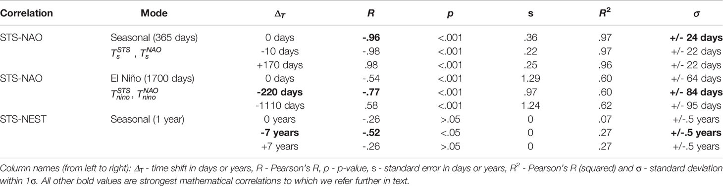
Table 1 Correlation between sea turtle sightings (STS) in Madeira, Hurrell North Atlantic Oscilation Index (NAO) and nests on core index beaches in peninsular Florida (NEST).

STS-NAO Correlation (seasonal mode). To verify interdependence between two signals, we apply a linear regression method based on the least squares, to STS (as dependent variable) and NAO (as independent variable). Both STS and NAO signals were filtered to extract their amplitude modulated seasonal components (T_s = 365 days). $T_s^{STS}$ and $T_s^{NAO}$ were filtered out by using 1 × BP 350 - 380 days. The very narrow band window is used in order to extract the unmodified seasonal components (which does not represent the full signal). The obtained correlation results are depicted in Table 1 and Supplementary Figure 6 respectively. The correlation coefficient dependence on the time shift is shown in Supplementary Figure 6A. Without any STS shift, a strong negative linear relationship is observed (R = - .96, p < .001, Supplementary Figure 6B), where p is the p-value statistical significance. Further obtained R-squared was computed (R² = .97) with the standard deviation σ = ± 24 days (Supplementary Figure 6C). The STS time shift Δ_T = -10 days (R = - .98, p < .001, Supplementary Figure 6D) does not deviate significantly relative to the non-shifted case. On the other hand, a strong positive correlation was found for Δ_T = + 170 days (R = 0.98, p < .001, Supplementary Figure 6F) with uncertainty of 1 σ = ± 22 days. The components used in cross-correlation $T_s^{STS}$ and $T_s^{NAO}$ are shown in Supplementary Figure 6. These results indicate that there is a strong anti-correlation present between the STS and NAO signals. The loggerhead sea turtles thus increase traction with the decrease of NAO (T_m), which implies their migration to the locations with calm weather.

STS-NAO Correlation (El Niño mode). As in the previous correlation, we analyze the relation between the seasonal components in STS and NAO data. The difference here is in that we now cross-correlate the El Niño modes (T_nino ~ 1700 days ~ 4.7 years) which we detect in the envelopes of seasonal components. The STS component $T_{nino}^{STS}$ was obtained with the following procedure: (i) 1 × BP 240 - 750 days; (ii) 1 × LP 1400 days - with demodulation; (iii) 1 × LP 1400 days; and (iv) 7 × HP 3000 days. Conversely, for the NAO component $T_{nino}^{NAO}$ we used similar steps: (i) 1 × BP 260 - 570 days; (ii) LP 1400 days - using the envelope of the signal (demodulation); (iii) LP 1400 days - additional low-pass to clear further interference from other side lobes; (iv) 5 × HP 3000 days - clearing large periods; and (v) 2 × HP 1500 days - solving further harmonic issues. Such strict band limits are used in order to encompass all components of the AM seasonal signal (the carrier and both side lobes), and also to filter out the specific mode from the envelope. The correlation coefficients in the case without and with STS shifts of T_nino modes are depicted in Figure 6A. Obtained correlations are given in Table 1 and in Figure 6 respectively. Moderate negative linear relationship was observed (R = - .54, p < .001, Figure 6B) with no STS shift with R² = .6, a = ± 64 days (Figure 6C), where again the NAO troughs match the peaks of STS, indicating loggerhead sea turtle increase as a response to lower NAO. Very strong negative relationship is also observed with the time shift of STS signal Δ_T = - 220 days (R = - .77, p < .001 seen in Figure 6D and R² = .6, σ = ± 84 days seen in Figure 6E). We also find a moderate strong positive relationship with STS time shift Δ_T = - 1110 days (R = - .58, p < .001 in Figure 6F and R² = .62, σ = ± 95 days in Figure 6G). STS peaks are seen as delayed reactions to NAO troughs and vice-versa (Figure 6H).

FIGURE 6

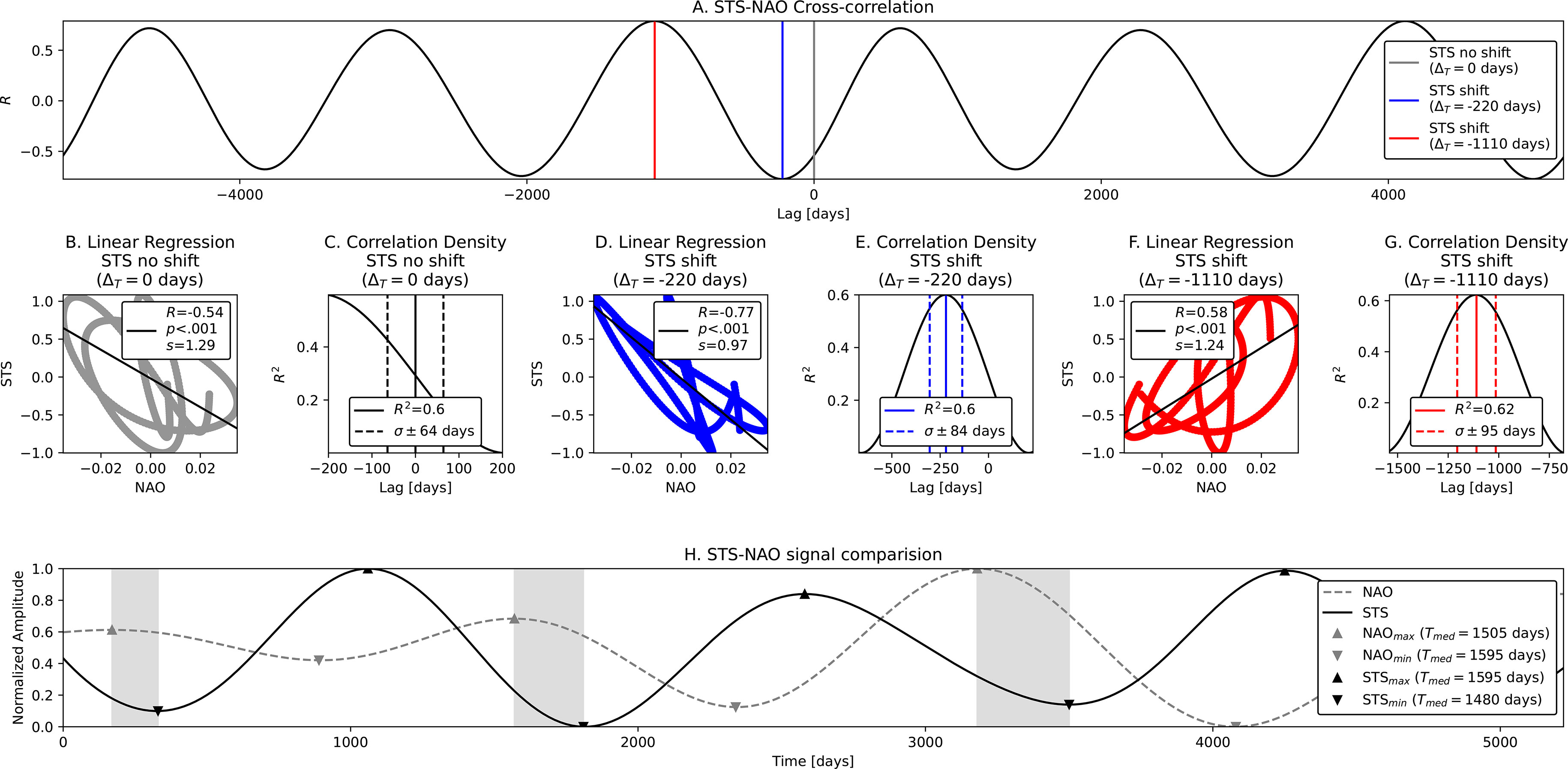
Figure 6 STS-NAO Cross-correlation and linear regression of El Niño modes – T_nino ~ 1700 days ~ 4.7 years. From top to bottom, left to right: (A) Correlation coefficients R for default STS (no shift) and shifted STS signals; (B–G) Linear regression results including coefficients of determination (R²) and error in days within 1σ; and (H) Positions of NAO peaks and STS troughs. Both El Niño modes are anticorrelated.

STS-NEST Correlation. Finally, we compare the STS signals with the loggerhead sea turtles nesting from Florida peninsula (NEST) using the yearly points of STS centered at July 1st (as the NEST data collection period). STS signal was filtered with following steps: (i) 1 × BP 240 - 750 days; (ii) 1 × LP 600 days - with demodulation; (iii) 3 × LP 1400 days; and (iv) 3 × HP 3000 days. Conversely, NEST signal was filtered with 3 × HP 10 years. Obtained correlations are depicted in Supplementary Figure 7 and Table 1, with highest correlation coefficient (R) shifts with Δ_T = 7 days (Supplementary Figure 7B). Using linear regression with no time shift (Δ_T = 0), although there is a mild correlation present (R = - .26 and R² = .07 in Supplementary Figure 7B, C), there is no statistically significant correlation (p > .5). Such is expected as sea turtles can not travel the greater distance from Florida to Madeira Island. However, 7-year time shift (Δ_T = - 7 years) provides statistical significance and strong negative correlation (R = - .52, R² = .27) as seen in Supplementary Figures 7D, E. Such indicates that sea turtles may have 7-year period since nesting until to be observed in Madeira Island. Additional correlation with Δ_T = 7 years showed mild negative correlation (R = - .26, R² = .27), however being not statistically significant (p > .05) as seen in Supplementary Figures 7F, G. Additional position of default and shifted STS signals, relative to NEST is seen in Supplementary Figure 7G, where the troughs of NEST match the STS peaks and vice-versa.

4 Discussion

This study provides a first in-water assessment of relative abundance of oceanic stage loggerhead turtles around Madeira Island, and the second for the North-Atlantic developmental habitats (Vandeperre et al., 2019), though a preliminary version of reported results was already integrated into the 1^st Portuguese National Report for the EU Marine Strategy Framework Directive  (S.R.A, 2014). Our relative abundance trend spans almost 15 years and provides an opportunity to study influencing factors. We show the direct evidence of basin-wide influence of climatic and oceanographic factors on local loggerhead abundance and distribution, emphasizing the fact that turtle conservation has to be addressed on basin-wide international levels. The oceanic life stage is the least studied life stage among all, where the quantitative assessment of abundance and distribution is key to understand turtle recruitment into subsequent life stages and habitats.

In both STS and NAO datasets, we found the strong seasonal component to be amplitude modulated by the longer (than one year) period modes. We detected the long period trend in STS data, and showed that it is composed of few independent periods of 850, 1700, and 2600 days, which altogether modulate the seasonal change in the number of turtle sightings. By the measured period, the first two components we relate to La Niña and El Niño, respectively. We refer to the longest period one as to some possibly new, still unexplained or undetected climate change trend. We also found the same long period components to appear in the envelope of the seasonal change in NAO index. Apart from the seasonal component and long periodicities, in STS time series we also detected an independent monthly oscillation which is being amplitude modulated by the seasonal and long period components.

The strong anti-correlation between the unmodified and non-shifted STS and NAO seasonal components, implies that loggerhead sea turtles increase traction with the decrease of NAO index (less turtles are sighted when NAO is positive), meaning that their migration is directed toward the warmer weather locations. Indeed, performed cross-correlation analysis between El Niño components which were previously detected in the envelopes of STS and NAO signals, showed the appearance of two maxima – one at the lag of ~ 7 months, and the other at the time shift of ~ 3 years. The shorter lag implies an anti-correlation between STS and NAO signals, suggesting the larger traction of loggerhead sea turtles with the decrease of air pressure difference. With an average turtle speed of half a knot, one circuit of the midocean North Atlantic Gyre would take around 440 days  (Carr, 1987). Since Florida to Madeira travel time would be half of this period, it may explain the detected ~ 7 months lag. On the other hand, the longer lag which leads to the positive correlation between STS and NAO signals, represents about half the time that turtles spend in oceanic life stage.

Interestingly, the rather strong maximum in the cross-correlation coefficient of cumulative NEST and STS time series reveals the time lag of ~ 7 years which finely coincides with the period of 7–9 years during which turtles stay in the eastern side of the Atlantic. The oscillation with the same period of ~ 7 years is also present in the long period pool of both, STS and NAO time series.

4.1 Index Credibility

Our relative abundance index took advantage of platforms of opportunity and records the number of turtles sighted per time spent searching per island sector, thus configuring a catch-per-unit-effort type of index. Giving that whale-watching companies have often more than 1 daily offshore trip, our temporal sampling density exceeds by greater extent most other applied methodologies, for instance distance sampling as in (Vandeperre et al., 2019), adding to statistical credibility. Since whale-watching trips varied little in their trip time, we have essentially a constant-effort scheme  (Quinn and Deriso, 1999) and thus a reliable and cost-effective population sampling methodology, for an otherwise challenging oceanic life stage sampling. For turtles, these types of indices have previously been used mainly to access bycatch rates  (Coelho et al., 2013; Carlson et al., 2016) and only recently have citizen science studies addressed population distribution and abundance  (Hof et al., 2017; Casale et al., 2020; Hanna et al., 2021). It furthermore represents an example of the contribution of ecotourism to conservation. However, since data recording was done by trained biologists or boat captains, our data cannot be considered citizen science proper (see Vohland et al. (2021) for definitions).

4.2 Population Trend

The population trend was derived using two very different methodologies (Figure 3). Both essentially coincided in overall curve shape, showing low population counts between 2010 and 2018 with marked lows in 2013 and 2018. Comparable datasets are from the Azores  (Vandeperre et al., 2019) and the Florida nesting (aforementioned NEST). The Azores dataset shows lows between 2005 and 2012 with a 3 year time lag to the Florida nesting data. Given the large distributional area of juvenile oceanic loggerheads from the Great Banks down to Mauritania  (Brazner and McMillan, 2008; McCarthy et al., 2010; Varo-Cruz et al., 2016; Freitas et al., 2018; Chambault et al., 2019; Freitas et al., 2019), local changes in population abundance can be caused by two complementary reasons: (1) a lower migration rate to oceanic habitats by juveniles from the production beaches or (2) spatial rearrangements due to oceanic conditions. Furthermore, different populations may use the waters in different ways.

4.3 Ocean-Atmosphere Influences

As widely roaming ectotherms sea turtles are sensitive to temperature variations and thus climate forcing and change  (Patrício et al., 2021). Our data indicate a strong STS and NAO seasonal trend components ($T_s^{STS}$ and $T_s^{NAO}$). Indeed, STS and NAO are anti-correlated, meaning that during positive NAO phases less turtles are sighted around Madeira. The influence of NAO on western Atlantic and Gulf pelagic communities is known (Stenseth et al., 2003; Roberts et al., 2019). Moreover, Johns et al. (2020) showed that Sargassum can be transported eastward during negative NAO phases and under extreme anomalous NAO conditions can reach the Canaries and Gibraltar. DuBois et al. (2020) described the influence of hurricanes on turtle hatchling dispersal within the Gulf of Mexico. Positive NAO indices are associated with more storms, where strengthened westerly winds are moved northwards and produce increased temperatures over northern Europe. Such causes dry anomalies and cooler than usual temperatures in the Mediterranean, while negative indices with the roughly the inverse  (Stenseth et al., 2003; Herceg-Bulić and Kucharski, 2014). The NAO index thus correlates with sea surface temperature (SST) in specific areas showing the tripole aspect of the NAO with negative correlation centers south of Greenland and in the western subtropics and a positive center off the US east coast  (Rodwell et al., 1999). Storm-forced dispersal of loggerheads, though not linked to NAO, was shown by Monzón-Argüello et al. (2012). They are also associated with reduced water surface layer thickness and higher stratification in the western part of the subtropical gyre and the Sargasso Sea  (Visbeck et al., 2003). Off New England positive NAO raises SST and affects local cod recruitment  (Meng et al., 2016). Warmer SST can induce turtles to migrate further North as found by  (Griffin et al., 2019), and thus be prone to a higher probability of cold-stunning when conditions change. Migrating further North may also be a behavioral adaptation to search for more productive colder waters as found by Plotkin (2010) for Olive Ridley’s in the eastern tropical Pacific. On the eastern North Atlantic and Mediterranean, positive NAO phases are associated with increased turtle stranding events  (Báez et al., 2011). NAO even seems to influence turtles in the eastern tropical Atlantic further south  (Báez et al., 2018).

We here found El Niño components in both STS and NAO signals ($T_{nino}^{STS}$ and $T_{nino}^{NAO}$) using the same WT/FFT spectral analysis and DSP techniques. These components are being lagged at ~ 7 months (anti-correlation) and ~ 3 years (correlation). The El Niño Southern Oscillation (ENSO) has global effects that also influence the North Atlantic, for instance affecting the path of the Gulf Stream with a time lag of 2 years  (Taylor and Stephens, 1998; Taylor et al., 1998). Bjorndal et al. (2017) showed that ecological regime shifts were influenced by unusually strong ENSO events and reduced turtle growth rates in the North and South Atlantic. As DuBois et al. (2020) wrote: “Both subtle differences in the position of oceanographic features (such as meandering currents) and major disturbances (such as hurricanes) can greatly alter dispersal outcomes.” As a result this will affect local abundances of sea turtles as those we measured in Madeira waters in the present study, driven by basin wide and larger climatic forcing. This is specially true if we consider that turtles are active swimmers, and not passive dispersers  (Dellinger, 1998; McCarthy et al., 2010; Putman and Mansfield, 2015; Freitas et al., 2018; Freitas et al., 2019) and will look up their best habitat given the environmental cues available to them.

4.4 Nesting Data and STS

Our STS data appears to be correlated with the NEST data form the Florida Index Nesting Beaches. However, in contrast to the findings of Vandeperre et al. (2019) who found a time lag of ~ 3 years, our time lag was double that amount with its ~ 7 years. This coincides with 7+ year average duration of the oceanic life stage (Bjorndal et al., 2003a). Why this might be so is unclear to us. The production beaches add on average 1/7^th each year to the oceanic turtle population, producing a regular turnover, and thus one year’s production should not influence overall abundance too much. However, Madeira waters serve as confluence developmental habitat for turtle from other origins as well, namely the Cape Verde Islands  (Lino et al., 2010; Marco et al., 2012; Marco, 2013), and these inputs probably influence the sightings at Madeira. Our satellite tracking data  (McCarthy et al., 2010; Freitas et al., 2018; Freitas et al., 2019) showed clearly that turtles tagged at summer onset migrated preferentially northward towards the Azores, while those tagged after the summer preferentially migrated SE towards the Canary Islands and Cape Verde. Interestingly enough the oscillation with very similar period of ~ 7 years was detected in the long period pool of both, STS and NAO time series.

4.5 Limitations and Future Work

Several planned studies can expand the present analysis. Some potential explanatory variables need testing: (1) the Cape Verde nesting data are needed which we could not secure for our time window, (2) lunar cycles may also prove relevant and (3) we should also check for longer timescale oscillations like the Arctic Oscillation (AO) that influences synchronously the whole Northern Hemisphere  (Beaugrand et al., 2015). Furthermore, since estimated turtle size was recorded, it would be important to check if size classes are affected differentially by climatic forcing or if the smallest size class has a stronger influence from nesting beaches  (Mansfield et al., 2014). Oceanic stage turtle movements are still poorly understood. Combined individual decisions results in collective movements through the interaction of biological processes and physical processes. Passive drift and active swimming (Polovina et al., 2000; Putman and Mansfield 2015) maintain turtles within appropriate habitat boundaries (Putman et al., 2012). Overall, and mainly for conservation purposes, it would be important to obtain a better picture of more or less synchronous area shifts of oceanic turtles within the North Atlantic which the present paper hints to, and for this more locations should be sampled in comparative ways.

4.6 Conclusions

Turtle populations are typically monitored by using the nesting data, including in-water and remote sensing studies  (Kobayashi et al., 2008; National Research Council, 2010). Such species are large organisms with long lifespans which produce large numbers of unnurtured offspring  (Hendrickson, 1980). A high mortality seems to occur around the transition to pelagic life  (Bjorndal et al., 2003b; Sasso and Epperly, 2007; Salmon and Scholl, 2014), thus making the monitoring of oceanic turtles an important tool to access both, their population status, as well as, the good environmental status of the high seas. To do this effectively, natural causes of the variation have to be understood and separated from anthropogenic causes. The present paper shows that in-water monitoring of juvenile oceanic loggerheads is feasible by using the platforms of opportunity and relative abundances. This points the way toward the implementation of more monitoring programs. Indeed, such programs can cover the wider spatial areas, since relative abundances are much more cost-effective to acquire, compared to the absolute abundances. Our results point to possible natural causes of the detected variation. These different variation time scales were only detectable by using the spectral analysis, a method not typically used in population assessments. Understanding natural causes of the population abundance variation is therefore critical to address anthropogenic factors more directly, e.g. fisheries bycatch or marine litter impact.

Data Availability Statement

The raw data supporting the conclusions of this article will be made available by the authors, without undue reservation.

Ethics Statement

Ethical review and approval was not required for the animal study because turtles were not handled, only spotted and counted, thus obviating the need for ethics approval according to legislation.

Author Contributions

TD designed the study, sampled the data and conducted STL analysis. VZ and MR performed spectral analysis, performing cross-correlation and applying Digital Signal Processing (DSP) techniques. All authors contributed to the article and approved the submitted version.

Funding

The work of MR was partially supported by the grants LARGESCALE (PTDC/CCICIF/32474/2017), INTERWHALE (PTDC/CCI-COM/0450/2020) and INTERTAGUA (MAC2/1.1.a/385) by FCT, MCTES, PIDDAC, and MAC-INTERREG funding respectively. The work of VZ was financially supported by the Ministry of Education, Science and Technological Development of the Republic of Serbia through the contract No. 451-03-68/2022-14/200104. This study had the support of FCT through the strategic project UIDB/04292/2020 awarded to MARE and through project LA/P/0069/2020 granted to the Associate Laboratory ARNET. Work is cofunded by the project NORTE-01-0246-FEDER-000063, supported by Norte Portugal Regional Operational Programme (NORTE2020), under the PORTUGAL 2020 Partnership Agreement, through the European Regional Development Fund (ERDF).

Conflict of Interest

The authors declare that the research was conducted in the absence of any commercial or financial relationships that could be construed as a potential conflict of interest.

Publisher’s Note

All claims expressed in this article are solely those of the authors and do not necessarily represent those of their affiliated organizations, or those of the publisher, the editors and the reviewers. Any product that may be evaluated in this article, or claim that may be made by its manufacturer, is not guaranteed or endorsed by the publisher.

Acknowledgments

Authors are thankful for the suggestions by the anonymous reviewers. We are most grateful to the companies Lobosonda, VMT and Rota dos Cetáceos, their managers, and mainly their crews for providing the original data.

Supplementary Material

The Supplementary Material for this article can be found online at: https://www.frontiersin.org/articles/10.3389/fmars.2022.877636/full#supplementary-material

Footnotes

1. ^ NAO dataset: http://www.cpc.ncep.noaa.gov/products/precip/CWlink/pna/norm.nao.monthly.b5001.current.ascii.
2. ^ NEST dataset: https://myfwc.com/research/wildlife/sea-turtles/nesting/beach-survey-totals/
3. ^ The spectrum of the amplitude modulated signal whose average value is zero, is composed of a carrier and two side lobes. If the modulated signal has no negative part (thus having the constant and positive average value), the frequency information of the modulating signal (the envelope spectrum) is not only contained in the two side lobes, but it is also present as an additional low-frequency band in its original form.
4. ^ A time delay introduced between the signals, for which their cross-correlation coefficient reaches its maximum value.
5. ^ The criteria that we used to determine whether some period is a harmonic or an independent mode, lies in the property of the phase of the mode itself, i.e. if the mode is coupled to the observed fundamental period as its harmonic – it thus makes the fundamental oscillation to appear as a more sharp change, or, if the mode is superimposed over that period – it therefore appears as being simply added over the fundamental oscillation.
6. ^ La Niña has a period of 2–4 years, while El Niño is 2–7 years.
7. ^ We use terms ”shift” and “lag” for the same meaning indicating the delay of the signal by amount of time (Δ_T).

References

Alves J. M., Caldeira R. M., Miranda P. M. (2020). Dynamics and Oceanic Response of the Madeira Tip-Jets. Q. J. R. Meteorol. Soc. 146, 3048–3063. doi: 10.1002/qj.3825

CrossRef Full Text | Google Scholar

Avens L., Goshe L., Coggins L., Snover M., Pajuelo M., Bjorndal K., et al. (2015). Age and Size at Maturation and Adult-Stage Duration for Loggerhead Sea Turtles in the Western North Atlantic. Mar. Biol. 162, 1749–1767. doi: 10.1007/s00227-015-2705-x

CrossRef Full Text | Google Scholar

Avens L., Goshe L. R., Pajuelo M., Bjorndal K. A., MacDonald B. D., Lemons G. E., et al. (2013). Complementary Skeletochronology and Stable Isotope Analyses Offer New Insight Into Juvenile Loggerhead Sea Turtle Oceanic Stage Duration and Growth Dynamics. Mar. Ecol. Prog. Ser. 491, 235–251. doi: 10.3354/meps10454

CrossRef Full Text | Google Scholar

Báez J. C., Bellido J. J., Ferri-Yáñez F., Castillo J. J., Mart´ın J. J., Mons J. L., et al. (2011). The North Atlantic Oscillation and Sea Surface Temperature Affect Loggerhead Abundance Around the Strait of Gibraltar. Sci. Mar. 75, 571–575. doi: 10.3989/scimar.2011.75n3571

CrossRef Full Text | Google Scholar

Ba´ez J. C., Macías D., Puerto M. A., Camin˜ as J. A., Ortiz de Urbina J. M. (2018). North Atlantic Oscillation Leads to the Differential Interannual Pattern Distribution of Sea Turtles From Tropical Atlantic Ocean. Collect. Vol. Sci. Pap. ICCAT 74, 3692–3697.

Google Scholar

Beaugrand G., Conversi A., Chiba S., Edwards M., Fonda-Umani S., Greene C., et al. (2015). Synchronous Marine Pelagic Regime Shifts in the Northern Hemisphere. Philos. Trans. R. Soc. B.: Biol. Sci. 370, 20130272. doi: 10.1098/rstb.2013.0272

CrossRef Full Text | Google Scholar

Bjorndal K. A., Bolten A. B., Chaloupka M., Saba V. S., Bellini C., Marcovaldi M. A. G., et al. (2017). Ecological Regime Shift Drives Declining Growth Rates of Sea Turtles Throughout the West Atlantic. Glob. Chang. Biol. 23, 4556–4568. doi: 10.1111/gcb.13712

PubMed Abstract | CrossRef Full Text | Google Scholar

Bjorndal K. A., Bolten A. B., Dellinger T., Delgado C., Martins H. R. (2003a). Compensatory Growth in Oceanic Loggerhead Sea Turtles: Response to a Stochastic Environment. Ecology 84, 1237–1249. doi: 10.1890/0012-9658(2003)084[1237:CGIOLS]2.0.CO;2

CrossRef Full Text | Google Scholar

Bjorndal K. A., Bolten A. B., Martins H. R. (2003b). Estimates of Survival Probabilities for Oceanic-Stage Loggerhead Sea Turtles (Caretta Caretta) in the North Atlantic. Fish. Bull. 101, 732–736.

Google Scholar

Bjorndal K., Bowen B., Chaloupka M., Crowder L., Heppell S., Jones C., et al. (2011). Better Science Needed for Restoration in the Gulf of Mexico. Science 331, 537–538. doi: 10.1126/science.1199935

PubMed Abstract | CrossRef Full Text | Google Scholar

Bolten A. B. (2003a). “Active Swimmers - Passive Drifters,” in The Oceanic Juvenile Stage of Loggerheads in the Atlantic System (Chapter 4) (Washington, D.C., USA: Smithsonian Institution Press), 63–78.

Google Scholar

Bolten A. B. (2003b). “Variation in Sea Turtle Life History Patterns,” in Neritic vs. Oceanic Developmental Stages(Chpt. 9), vol. vol. II. (Boca Raton, USA: CRC Press), 243–257.

Google Scholar

Bolten A. B., Bjorndal K. A., Martins H. R., Dellinger T., Biscoito M. J., Encalada S. E., et al. (1998). Transatlantic Developmental Migrations of Loggerhead Sea Turtles Demonstrated by Mtdna Sequence Analysis. Ecol. Appl. 8, 1–7. doi: 10.1890/1051-0761(1998)008[0001:TDMOLS]2.0.CO;2

CrossRef Full Text | Google Scholar

Brazner J. C., McMillan J. (2008). Loggerhead Turtle (Caretta Caretta) Bycatch in Canadian Pelagic Longline Fisheries: Relative Importance in the Western North Atlantic and Opportunities for Mitigation. Fish. Res. 91, 310–324. doi: 10.1016/j.fishres.2007.12.023

CrossRef Full Text | Google Scholar

Brigham E. O., Morrow R. (1967). The Fast Fourier Transform. IEEE Spectr. 4, 63–70. doi: 10.1109/MSPEC.1967.5217220

CrossRef Full Text | Google Scholar

Caldeira R. M. A. (2019). Island Wakes. 3rd ed (Oxford: Academic Press), 83–91. doi: 10.1016/B978-0-12-409548-9.11614-8

CrossRef Full Text | Google Scholar

Caldeira R. M. A., Groom S., Miller P., Pilgrim D., Nezlin N. P. (2002). Sea-Surface Signatures of the Island Mass Effect Phenomena Around Madeira Island, Northeast Atlantic. Remote Sens. Environ. 80, 336–360. doi: 10.1016/S0034-4257(01)00316-9

CrossRef Full Text | Google Scholar

Caldeira R. M. A., Sangra P. (2012). Complex Geophysical Wake Flows. Ocean. Dyn. 62, 683–700. doi: 10.1007/s10236-012-0528-6

CrossRef Full Text | Google Scholar

Carlson J. K., Gulak S. J. B., Enzenauer M. P., Stokes L. W., Richards P. M. (2016). Characterizing Loggerhead Sea Turtle, Caretta Caretta, Bycatch in the Us Shark Bottom Longline Fishery. Bull. Mar. Sci. 92, 513–525. doi: 10.5343/bms.2016.1022

CrossRef Full Text | Google Scholar

Carr A. (1987). New Perspectives on the Pelagic Stage of Sea Turtle Development. Conserv. Biol. 1, 103–121. doi: 10.1111/j.1523-1739.1987.tb00020.x

CrossRef Full Text | Google Scholar

Casale P., Abbate G., Freggi D., Conte N., Oliverio M., Argano R. (2008). Foraging Ecology of Loggerhead Sea Turtles Caretta Caretta In the Central Mediterranean Sea: Evidence for a Relaxed Life History Model. Mar. Ecol. Prog. Ser. 372, 265–276. doi: 10.3354/meps07702

CrossRef Full Text | Google Scholar

Casale P., Ciccocioppo A., Vagnoli G., Rigoli A., Freggi D., Tolve L., et al. (2020). Citizen Science Helps Assessing Spatio-Temporal Distribution of Sea Turtles In Foraging Areas. Aquat. Conserv.: Mar. Freshw. Ecosyst. 30, 123–130. doi: 10.1002/aqc.3228

CrossRef Full Text | Google Scholar

Casale P., Tucker A. D. (2017). Caretta caretta (amended version of 2015 assessment). The IUCN Red List of Threatened Species 2017 e.t3897a119333622. doi: 10.2305/IUCN.UK.2017-2.RLTS,T3897A119333622.en

CrossRef Full Text | Google Scholar

Chambault P., Baudena A., Bjorndal K. A., Ar Santos M., Bolten A. B., Vandeperre F. (2019). Swirling in the Ocean: Immature Loggerhead Turtles Seasonally Target Old Anticyclonic Eddies at the Fringe of the North Atlantic Gyre. Prog. Oceanogr. 175, 345–358. doi: 10.1016/j.pocean.2019.05.005

CrossRef Full Text | Google Scholar

Chan K.-S., Ripley B. (2020). Tsa: Time Series Analysis. R Package Version 1.3 at https://CRAN.Rproject.org/package=TSA.

Google Scholar

Cleveland R. B., Cleveland W. S., McRae J. E., Terpenning I. (1990). Stl: A Seasonal-Trend Decomposition Procedure Based on Loess. J. Off. Stat 6, 3–73.

Google Scholar

Coelho R., Fernandez-Carvalho J., Santos M. N. (2013). A Review of Methods for Assessing the Impact of Fisheries On Sea Turtles. Collect. Vol. Sci. Pap. ICCAT 69, 1828–1859.

Google Scholar

Cowpertweit P. S. P., Metcalfe A. V. (2009). Introductory Time Series With R. Use R! (Dordrecht, NL: Springer). doi: 10.1007/978-0-387-88698-5

CrossRef Full Text | Google Scholar

Crouse D. T., Crowder L. B., Caswell H. (1987). A Stage-Based Population Model for Loggerhead Sea Turtles and Implications for Conservation. Ecology 6, 1412–1423. doi: 10.2307/1939225

CrossRef Full Text | Google Scholar

Delgado C., Canário A., Dellinger T. (2010). Sex Ratios of Loggerhead Sea Turtles Caretta Caretta During the Juvenile Pelagic Stage. Mar. Biol. 157, 979–990. doi: 10.1007/s00227-009-1378-8

CrossRef Full Text | Google Scholar

Dellinger T. (1998). The Wandering Turtles of the Atlantic. Sci. Am. Present. 9, 88–91.

Google Scholar

Dellinger T., Davenport J., Wirtz P. (1997). Comparisons of Social Structure of Columbus Crabs Living on Loggerhead Sea Turtles and Inanimate Flotsam. J. Mar. Biol. Assoc. Uni. Kingd. 77, 185–194. doi: 10.1017/S0025315400033865

CrossRef Full Text | Google Scholar

DuBois M. J., Putman N. F., Piacenza S. E. (2020). Hurricane Frequency and Intensity may Decrease Dispersal of Kemp’s Ridley Sea Turtle Hatchlings in the Gulf of Mexico. Front. Mar. Sci. 7. doi: 10.3389/fmars.2020.00301

CrossRef Full Text | Google Scholar

Fox J., Weisberg S. (2019). An R Companion to Applied Regression. 3rd ed (Thousand Oaks, CA: SAGE Publications).

Google Scholar

Freitas C., Caldeira R., Dellinger T. (2019). Surface Behavior of Pelagic Juvenile Loggerhead Sea Turtles in the Eastern North Atlantic. J. Exp. Mar. Biol. Ecol. 510, 73–80. doi: 10.1016/j.jembe.2018.10.006

CrossRef Full Text | Google Scholar

Freitas C., Caldeira R., Reis J., Dellinger T. (2018). Foraging Behavior of Juvenile Loggerhead Sea Turtles in the Open Ocean: From Levy Exploration to Area-Restricted Search. Mar. Ecol. Prog. Ser. 595, 203–215. doi: 10.3354/meps12581

CrossRef Full Text | Google Scholar

Furey N. B., Armstrong J. B., Beauchamp D. A., Hinch S. G. (2018). Migratory Coupling Between Predators and Prey. Nat. Ecol. Evol. 2, 1846–1853. doi: 10.1038/s41559-018-0711-3

PubMed Abstract | CrossRef Full Text | Google Scholar

Geldmacher J., Bogaard P., Hoernle K., Schmincke H. (2000). The 40ar/39ar Age Dating of the Madeira Archipelago and Hotspot Track (Eastern North Atlantic). Geochem. Geophys. Geosyst. 1, 109–122. doi: 10.1029/1999GC000018

CrossRef Full Text | Google Scholar

Griffin L. P., Griffin C. R., Finn J. T., Prescott R. L., Faherty M., Still B. M., et al. (2019). Warming Seas Increase Cold-Stunning Events for Kemp’s Ridley Sea Turtles in the Northwest Atlantic. PLoS One 14, e0211503. doi: 10.1371/journal.pone.0211503

PubMed Abstract | CrossRef Full Text | Google Scholar

Hanna M. E., Chandler E. M., Semmens B. X., Eguchi T., Lemons G. E., Seminoff J. A. (2021). Citizen-Sourced Sightings and Underwater Photography Reveal Novel Insights About Green Sea Turtle Distribution and Ecology in Southern California. Front. Mar. Sci. 8. doi: 10.3389/fmars.2021.671061

PubMed Abstract | CrossRef Full Text | Google Scholar

Hays G. C., Scott R. (2013). Global Patterns for Upper Ceilings on Migration Distance in Sea Turtles and Comparisons With Fish, Birds and Mammals. Funct. Ecol. 27, 748–756. doi: 10.1111/1365-2435.12073

CrossRef Full Text | Google Scholar

Hendrickson J. R. (1980). The Ecological Strategies of Sea Turtles. Am. Zool. 20, 597–608. doi: 10.1093/icb/20.3.597

CrossRef Full Text | Google Scholar

Herceg-Bulić I., Kucharski F. (2014). North Atlantic Ssts as a Link Between the Wintertime Nao and the Following Spring Climate. J. Climate 27, 186–201. doi: 10.1175/jcli-d-12-00273.1

CrossRef Full Text | Google Scholar

Hof C. A. M., Smallwood E., Meager J., Bell I. P. (2017). First Citizen-Science Population Abundance and Growth Rate Estimates for Green Sea Turtles Chelonia Mydas Foraging in the Northern Great Barrier Reef, Australia. Mar. Ecol. Prog. Ser. 574, 181–191. doi: 10.3354/meps12173

CrossRef Full Text | Google Scholar

Houghton J. D., Callow M. J., Hays G. C. (2003). Habitat Utilization by Juvenile Hawksbill Turtles (Eretmochelys Imbricata, Linnaeus 1766) Around a Shallow Water Coral Reef. J. Natural Histor. 37, 1269–1280. doi: 10.1080/00222930110104276

CrossRef Full Text | Google Scholar

Hurrell J. W., Deser C. (2010). North Atlantic Climate Variability: The Role of the North Atlantic Oscillation. J. Mar. Syst. 79, 231–244. doi: 10.1016/j.jmarsys.2009.11.002

CrossRef Full Text | Google Scholar

IFAW (2009). “Whale Watching Worldwide,” in Tourism Numbers, Expenditures and Expanding Economic Benefits (Yarmouth Port, MA:International Fund for Animal Welfare). Available at: http://www.ifaw.org/Publications/Program_Publications/Whales/asset_upload_file841_55365.pdf

Google Scholar

Johns E. M., Lumpkin R., Putman N. F., Smith R. H., Muller-Karger F. E., T. Rueda-Roa D., et al. (2020). The Establishment of a Pelagic Sargassum Population in the Tropical Atlantic: Biological Consequences of a Basin-Scale Long Distance Dispersal Event. Prog. Oceanogr. 182, 102269. doi: 10.1016/j.pocean.2020.102269

CrossRef Full Text | Google Scholar

Kobayashi D. R., Polovina J. J., Parker D. M., Kamezaki N., Cheng I.-J., Uchida I., et al. (2008). Pelagic Habitat Characterization of Loggerhead Sea Turtles, Caretta Caretta, in the North Pacific Ocean, (1997–2006): Insights From Satellite Tag Tracking and Remotely Sensed Data. J. Exp. Mar. Biol. Ecol. 356, 96–114. doi: 10.1016/j.jembe.2007.12.019

CrossRef Full Text | Google Scholar

Krasovskaya S. (2018). Economic Contribution of the Whale-Watching Industry for the Madeira Archipelago (Masters Thesis in Ecotourism, University of Madeira:Funchal, Portugal) at https://digituma.uma.pt/bitstream/10400.13/1852/1/MestradoSvetlana%20Krasovskaya.pdf

Google Scholar

Lascelles B., Notarbartolo Di Sciara G., Agardy T., Cuttelod A., Eckert S., Glowka L., et al. (2014). Migratory Marine Species: Their Status, Threats and Conservation Management Needs. Aquat. Conserv.: Mar. Freshw. Ecosyst. 24, 111–127. doi: 10.1002/aqc.2512

CrossRef Full Text | Google Scholar

Lino S. P. P., Gonc¸alves E., Cozens J. (2010). The Loggerhead Sea Turtle (Caretta Caretta) on Sal Island, Cape Verde: Nesting Activity and Beach Surveillance In 2009. Arquipe´lag - Life Mar. Sci. 27, 59–63.

Google Scholar

Mansfield K. L., Wyneken J., Porter W. P., Luo J. (2014). First Satellite Tracks of Neonate Sea Turtles Redefine the ‘Lost Years’ Oceanic Niche. Proc. R. Soc. Lond. Ser. B.: Biol. Sci. 281, 1–9. doi: 10.1098/rspb.2013.3039

CrossRef Full Text | Google Scholar

Marco A. (2013). The 2013 Loggerhead Nesting Season in Boavista. Zool. News 3, 2.

Google Scholar

Marco A., Abella E., Liria-Loza A., Martins S., Lopez O., Jimenez-Bordon S., et al. (2012). Abundance and Exploitation of Loggerhead Turtles Nesting in Boa Vista Island, Cape Verde: The Only Substantial Rookery in the Eastern Atlantic. Anim. Conserv. 15, 351–360. doi: 10.1111/j.1469-1795.2012.00547.x

CrossRef Full Text | Google Scholar

McCarthy A. L., Heppell S., Royer F., Freitas C., Dellinger T. (2010). Identification of Likely Foraging Habitat of Pelagic Loggerhead Sea Turtles (Caretta Caretta) in the North Atlantic Through Analysis of Telemetry Track Sinuosity. Prog. In. Oceanogr. 86, 224–231. doi: 10.1016/j.pocean.2010.04.009

CrossRef Full Text | Google Scholar

McClellan C. M., Read A. J. (2007). Complexity and Variation in Loggerhead Sea Turtle Life History. Biol. Lett. 3, 592–594. doi: 10.1098/rsbl.2007.0355

PubMed Abstract | CrossRef Full Text | Google Scholar

Meng K., Oremus K., Gaines S. (2016). New England Cod Collapse and the Climate. PLoS One 11, e0158487. doi: 10.1371/journal.pone.0158487

PubMed Abstract | CrossRef Full Text | Google Scholar

Monzón-Argüello C., Dell’Amico F., Moriniere P., Marco A., Lopez-Jurado L. F., Hays G. C., et al. (2012). Lost at Sea: Genetic, Oceanographic and Meteorological Evidence for Storm-Forced Dispersal. J. R. Soc. Interface 9, 1725–1732. doi: 10.1098/rsif.2011.0788

PubMed Abstract | CrossRef Full Text | Google Scholar

Monzón-Argüello C., Rico C., Carreras C., Calabuig P., Marco A., Felipe Lopez-Jurado L. (2009). Variation in Spatial Distribution of Juvenile Loggerhead Turtles in the Eastern Atlantic and Western Mediterranean Sea. J. Exp. Mar. Biol. Ecol. 373, 79–86. doi: 10.1016/j.jembe.2009.03.007

CrossRef Full Text | Google Scholar

Narciso A., Caldeira R., Reis J., Hoppenrath M., Cacha˜o M., Kaufmann M. (2019). The Effect of a Transient Frontal Zone on the Spatial Distribution of Extant Coccolithophores Around the Madeira Archipelago (Northeast Atlantic). Estuar. Coast. Shelf. Sci. 223, 25–38. doi: 10.1016/j.ecss.2019.04.014

CrossRef Full Text | Google Scholar

National Research Council (2010). Assessment of Sea-Turtle Status and Trends: Integrating Demography and Abundance (Washington, DC: National Academies Press). doi: 10.17226/12889

CrossRef Full Text | Google Scholar

Nunes N. J., Radeta M., Nisi V. (2020). “Enhancing Whale Watching With Mobile Apps and Streaming Passive Acoustics,” in International Conference on Entertainment Computing (Springer), 205–222. doi: 10.1007/978-3-030-65736-9_18

CrossRef Full Text | Google Scholar

Patrício A. R., Hawkes L. A., Monsinjon J. R., Godley B. J., Fuentes M. (2021). Climate Change and Marine Turtles: Recent Advances and Future Directions. Endang. Specie. Res. 44, 363–395. doi: 10.3354/esr01110

CrossRef Full Text | Google Scholar

Peltier H., Ridoux V. (2015). Marine Megavertebrates Adrift: A Framework for the Interpretation of Stranding Data in Perspective of the European Marine Strategy Framework Directive and Other Regional Agreements. Environ. Sci. Policy 54, 240–247. doi: 10.1016/j.envsci.2015.07.013

CrossRef Full Text | Google Scholar

Pipa T., Atchoi E., Silva C., Be´cares J., Gil M., Freitas L., et al. (2019). “MISTIC SEAS II: Applying a Subregional Coherent and Coordinated Approach to the Monitoring and Assessment of Marine Biodiversity in Macaronesia for the Second Cycle of the MSFD. Final Technical Report (TRWP1): Workpackage 1 - Monitoring Programs and Data Gathering,” in Tech. Rep., European Commission, pp.339. doi: 10.13140/RG.2.2.17231.10407

CrossRef Full Text | Google Scholar

Plotkin P. T. (2010). Nomadic Behaviour of the Highly Migratory Olive Ridley Sea Turtle Lepidochelys Olivacea in the Eastern Tropical Pacific Ocean. Endang. Specie. Res. 13, 33–40. doi: 10.3354/esr00314

CrossRef Full Text | Google Scholar

Polovina J. J., Kobayashi D. R., Parker D. M., Seki M. P., Balazs G. H. (2000). Turtles on the Edge: Movement of Loggerhead Turtles (Caretta Caretta) Along Oceanic Fronts, Spanning Longline Fishing Grounds in the Central North Pacific 1997–1998. Fish. Oceanogr. 9, 71–82. doi: 10.1046/j.1365-2419.2000.00123.x

CrossRef Full Text | Google Scholar

Putman N., Mansfield K. (2015). Direct Evidence of Swimming Demonstrates Active Dispersal in the Sea Turtle “Lost Years”. Curr. Biol. 25, 1221–1227. doi: 10.1016/j.cub.2015.03.014

PubMed Abstract | CrossRef Full Text | Google Scholar

Putman N. F., Seney E. E., Verley P., Shaver D. J., Lo´ pez-Castro M. C., Cook M., et al. (2020). Predicted Distributions and Abundances of the Sea Turtle ‘Lost Years’ in the Western North Atlantic Ocean. Ecography 43, 506–517. doi: 10.1111/ecog.04929

CrossRef Full Text | Google Scholar

Putman N. F., Verley P., Shay T. J., Lohmann K. J. (2012). Simulating Transoceanic Migrations of Young Loggerhead Sea Turtles: Merging Magnetic Navigation Behavior With an Ocean Circulation Model. J. Exp. Biol. 215, 1863–1870. doi: 10.1242/jeb.067587

PubMed Abstract | CrossRef Full Text | Google Scholar

Quinn T. J., Deriso R. B. (1999). “Quantitative Fish Dynamics,” in Biological Resource Management Series (New York, NY: Oxford University Press).

Google Scholar

Radeta M., Nunes N. J., Vasconcelos D., Nisi V. (2018). “Poseidon-Passive-Acoustic Ocean Sensor for Entertainment and Interactive Data-Gathering in Opportunistic Nautical-Activities,” in Proceedings of the2018 Designing Interactive Systems Conference. 999–1011. doi: 10.1145/3196709.3196752

CrossRef Full Text | Google Scholar

R Development Core Team (2021). R Language Definition, Version 4.1.2 (2021-11-01. R Foundation for Statistical Computing. http://cran.r-project.org/doc/manuals/R-lang.pdf

Google Scholar

Regional da Madeira A. (2013). Decreto Legislativo Regional N.° 15/2013/M De 14 De Maio: Aprova O Regulamento Da Atividade De Observac¸A˜o De Vertebrados Marinhos Na Regia˜o Auto´ Noma Da Madeira. Jorn. Oficial. Da. Regia˜. O. Auto´. Noma. Da. Madeira. I. Se´rie. 57, 2–12.

Google Scholar

Roberts S. M., Boustany A. M., Halpin P. N., Rykaczewski R. R. (2019). Cyclical Climate Oscillation Alters Species Statistical Relationships With Local Habitat. Mar. Ecol. Prog. Ser. 614, 159–171. doi: 10.3354/meps12890

CrossRef Full Text | Google Scholar

Rodwell M., Rowell D., Folland C. (1999). Oceanic Forcing of the Wintertime North Atlantic Oscillation and European Climate. Nature 398, 320–323. doi: 10.1038/18648

CrossRef Full Text | Google Scholar

Saavedra C., Begoña Santos M., Valcarce P., Freitas L., Silva M., Pipa T., et al. (2018). “MISTIC SEAS Ii,” in Macaronesia Roof Report. Tech. Rep., European Commission, pp. 116 at https://misticseas3.com/sites/default/files/materialdivulgativo/macaronesian_roof_report_en.pdf

Google Scholar

Salmon M., Scholl J. (2014). Allometric Growth in Juvenile Marine Turtles: Possible Role as an Antipredator Adaptation. Zoology 117, 131–138. doi: 10.1016/j.zool.2013.11.004

PubMed Abstract | CrossRef Full Text | Google Scholar

Sambolino A., Alves F., Fernandez M., Krakauer A. B., Ferreira R., Dinis A. (2022). Spatial and Temporal Characterization of the Exposure of Island-Associated Cetacean Populations To Whale- Watching in Madeira Island (Ne Atlantic). Reg. Stud. Mar. Sci. 49, 102084. doi: 10.1016/j.rsma.2021.102084

CrossRef Full Text | Google Scholar

Sasso C. R., Epperly S. P. (2007). Survival of Pelagic Juvenile Loggerhead Turtles in the Open Ocean. J. Wildl. Manage. 71, 1830–1835. doi: 10.2193/2006-448

CrossRef Full Text | Google Scholar

Sequeira M., Elejabeitia C., Silva M., Dinis A., Stephanis R., Urquiola E., et al. (2009). Review of Whalewatching Activities in Mainland Portugal, the Azores, Madeira and Canary Archipelagos and the Strait of Gibraltar J Cetacean Res. Manage SC61/WW11

Google Scholar

S.R.A (2014). Diretiva Quadro Estrate´gia Marinha: Estrate´gia Marinha Para a Subdivisa˜ O Da Madeira (Funchal:Secretaria Regional do Ambiente e dos Recursos Naturais), pp. 463. Available at: https://www.dgrm.mm.gov.pt/as-pem-diretiva-quadro-estrategiamarinha#collapse__com_liferay_journal_content_web_portlet_JournalContentPortlet_INSTANCE_QFjQWpm5JsNv__3

Google Scholar

Stenseth N. C., Ottersen G., Hurrell J. W., Mysterud A., Lima M., Chan K. S., et al. (2003). Studying Climate Effects on Ecology Through the Use of Climate Indices: The North Atlantic Oscillation, El Nin˜ O Southern Oscillation and Beyond. Proc. R. Soc. Lond. Ser. B.: Biol. Sci. 270, 2087–2096.

Google Scholar

Taylor A. H., Jordan M. B., Stephens J. A. (1998). Gulf Stream Shifts Following Enso Events. Nature 393, 638. doi: 10.1038/31380

CrossRef Full Text | Google Scholar

Taylor A. H., Stephens J. A. (1998). The North Atlantic Oscillation and the Latitude of the Gulf Stream. Tellu. A.: Dyn. Meteorol. Oceanogr. 50, 134–142. doi: 10.3402/tellusa.v50i1.14517

CrossRef Full Text | Google Scholar

Torrence C., Compo G. P. (1998). A Practical Guide to Wavelet Analysis. Bull. Amer. Meteor. Soc 79, 61–78. doi: 10.1175/1520-0477(1998)079<0061:APGTWA>2.0.CO;2

CrossRef Full Text | Google Scholar

Trenberth K. E. (1997). The Definition of El Nino. Bull. Am. Meteorol. Soc. 78, 2771–2778. doi: 10.1175/1520-0477(1997)078<2771:TDOENO>2.0.CO;2

CrossRef Full Text | Google Scholar

Turtle Expert Working Group (2009). An Assessment of the Loggerhead Turtle Population in the Western Northern Atlantic Ocean, a Report of the Turtle Expert Working Group. NOAA Technical Memorandu NMFS-SEFSC 575, pp.1–131. https://repository.library.noaa.gov/view/noaa/3714.

Google Scholar

Vandeperre F., Parra H., Pham C. K., Machete M., Santos M., Bjorndal K. A., et al. (2019). Relative Abundance of Oceanic Juvenile Loggerhead Sea Turtles in Relation to Nest Production at Source Rookeries: Implications for Recruitment Dynamics. Sci. Rep. 9, 13019. doi: 10.1038/s41598-019-49434-0

PubMed Abstract | CrossRef Full Text | Google Scholar

Varo-Cruz N., Bermejo J. A., Calabuig P., Cejudo D., Godley B. J., Lo´ pez-Jurado L. F., et al. (2016). New Findings About the Spatial and Temporal Use of the Eastern Atlantic Ocean by Large Juvenile Loggerhead Turtles. Diversity Distri. 22, 481–492. doi: 10.1111/ddi.12413

CrossRef Full Text | Google Scholar

Visbeck M., Chassignet E. P., Curry R., Delworth T., Dickson B., Krahmann G. (2003). The Ocean’s Response to North Atlantic Oscillation Variability (Washington, DC: American Geophysical Union), 113–145. doi: 10.1029/GM134

CrossRef Full Text | Google Scholar

Vohland K., Land-Zandstra A., Ceccaroni L., Lemmens R., Perello´ J., Ponti M., et al. (2021). The Science of Citizen Science (Cham, Switzerland: Springer). doi: 10.1007/978-3-030-58278-4

CrossRef Full Text | Google Scholar

Wallace B. P., DiMatteo A. D., Bolten A. B., Chaloupka M. Y., Hutchinson B. J., Abreu-Grobois F. A., et al. (2011). Global Conservation Priorities for Marine Turtles. PLoS One 6(9), 1–14. doi: 10.1371/journal.pone.0024510

CrossRef Full Text | Google Scholar

Wallace B. P., DiMatteo A. D., Hurley B. J., Finkbeiner E. M., Bolten A. B., Chaloupka M. Y., et al. (2010). Regional Management Units for Marine Turtles: A Novel Framework for Prioritizing Conservation and Research Across Multiple Scales. PLoS One 5, 15465. doi: 10.1371/journal.pone.0015465

CrossRef Full Text | Google Scholar

Wickham H. (2007). Reshaping Data With the Reshape Package. J. Stat. Softw. 21, 1–20. doi: 10.18637/jss.v021.i12

CrossRef Full Text | Google Scholar

Wickham H., Franc¸ois R., Henry L., Mu¨ ller K. (2022). Dplyr: A Grammar of Data Manipulation. R Package Version 1.0.8.

Google Scholar

Witherington B., Herren R. M., Bresette M. (2006). Caretta Caretta – Loggerhead Sea Turtle (Lunenburg, MA: Chelonian Research Foundation), 74–89.

Google Scholar

World Meterological Organization (2012). Manual on Marine Meteorological Services. Vol. 2 – Regional Aspects (Geneva, Switzerland: WMO).

Google Scholar