Chasing the offshore wind farm wind-wake-induced upwelling/downwelling dipole

Introduction

The pelagic effects of offshore wind farm (OWF) foundations in the stratified North Sea have been analyzed by a combination of empirical and modeling studies (Carpenter et al., 2016; Floeter et al., 2017; Schultze et al., 2020; Dorrell et al., 2022). There are currently few empirical data showing how the presence of an OWF, which changes the wind stress at the sea surface, affects the upper ocean and pelagic ecosystem. Offshore wind farms (OWFs) convert kinetic wind energy into electricity, creating regions of reduced wind speed and high atmospheric turbulence intensity downstream of wind turbine arrays. Christiansen and Hasager (2005); Christiansen and Hasager (2006) were the first to describe these wind-wakes by synthetic aperture radar (SAR)-derived wind speed images and well-known wind farm wake photographs (Hasager et al., 2013). Numerical analyses by Broström (2008) triggered a series of modeling studies (Paskyabi and Fer, 2012; Paskyabi, 2015; Ludewig, 2015), which all predicted that a wind speed of 5–10 m s^-1 generates so-called upwelling/downwelling dipoles in a stratified ocean with vertical velocities exceeding 1 m day^-1. The generated oceanic response is predicted to extend several kilometers around the OWFs and to be strong enough to influence the local pelagic ecosystem, especially the surface mixed layer (SML). These studies formulated prerequisite conditions for the generation of an OWF wind-wake-induced upwelling/downwelling dipole: the characteristic width of the wind-wake has to be at least the internal radius of deformation (Broström, 2008), which is fulfilled for OWFs in the German Bight of the North Sea, as both are ~10 km (Chelton et al., 1998; Platis et al., 2018). An almost constant wind direction for at least ~8–10 h with moderate speeds (5–10 m s^-1) is the second condition which needs to be met (Ludewig, 2015). Other theoretically derived factors likely to influence the vertical velocities in OWF wind-wake-induced upwelling/downwelling dipoles are the size of the wind farm (Broström, 2008), surface waves and tidal advection (Paskyabi and Fer, 2012), and atmospheric stability (Platis et al., 2018).

Christiansen et al. (2022) forced a cross-scale hydrodynamic unstructured-grid model with a realistic temporally changing wind field. The authors observed that individual upwelling/downwelling dipoles shift their spatial positions, following the directional changes of their causative wind-wakes. Thereby in some cases, specific dipoles superimposed, either combining their effect or canceling/mitigating each other. Consequently, on the monthly average time scale Christiansen et al. (2022) obtained large-scale surface elevation dipoles with spatial dimensions of up to hundreds of kilometers in the German Bight, strong enough to structurally change the seasonal course of stratification strength.

Due to their ephemeral nature, empirical evidence of the underlying specific OWF wind-wake-induced upwelling/downwelling dipoles is lacking. Besides the necessary atmospheric and hydrodynamic conditions (i.e., stratification), contrasting quasi-synoptic water column surveys of the leeward area are required to fill this gap. In June 2016, we deployed a high-speed remotely operated towed vehicle (ROTV) to investigate the offshore wind farm wind-wake-induced upwelling/downwelling dipole.

Materials and methods

Data analysis

Data analysis and visualization were conducted using the software program R (R Core Team, 2022), the R-packages ‘‘ggplot2” Wickham (2016), “scales” (Wickham and Seidel, 2019), “NISTunits” (Gama, 2016), and “lubridate” (Grolemund and Wickham, 2011) as well as Ocean Data View 5.40 (ODV, Schlitzer, 2021). Data were gridded using the ODV-weighted average or ODV/DIVA method with automatic scale lengths (Troupin et al., 2012). We used the cmocean color maps within ODV following the guidelines of Thyng et al. (2016).

OWF operation

The two OWFs that were surveyed, Global Tech I (GTI) and BARD Offshore 1 (BARD), are located at a water depth of around 40 m in the German EEZ, and a distance of approximately 100 km offshore. Both OWFs had 80 wind power plants installed, whereby the number of turbines ready to operate varied over time (Figure 1). The available turbines start to operate, i.e., turn the blades and generate a wind-wake, at a wind speed of 4 m s⁻¹. On June 26, all GTI turbines had to be stopped around noon due to a technical reason. This complete GTI shutdown lasted for ~33 h until 9:00 UTC on June 27. During June 28, the number of operating turbines was stepwise increased to 59 and further on to 60–67 during the following 2 days. The number of operating turbines in BARD was quite stable over the entire survey time (mean: 72.64, cv: 2.4%, min: 69, max: 75), creating contrasting situations for our investigations: on June 27, BARD was generating a wind-wake, whereas the neighboring OWF GTI did not. During the subsequent days June 29 and June 30, both OWFs generated wind-wakes.

FIGURE 1

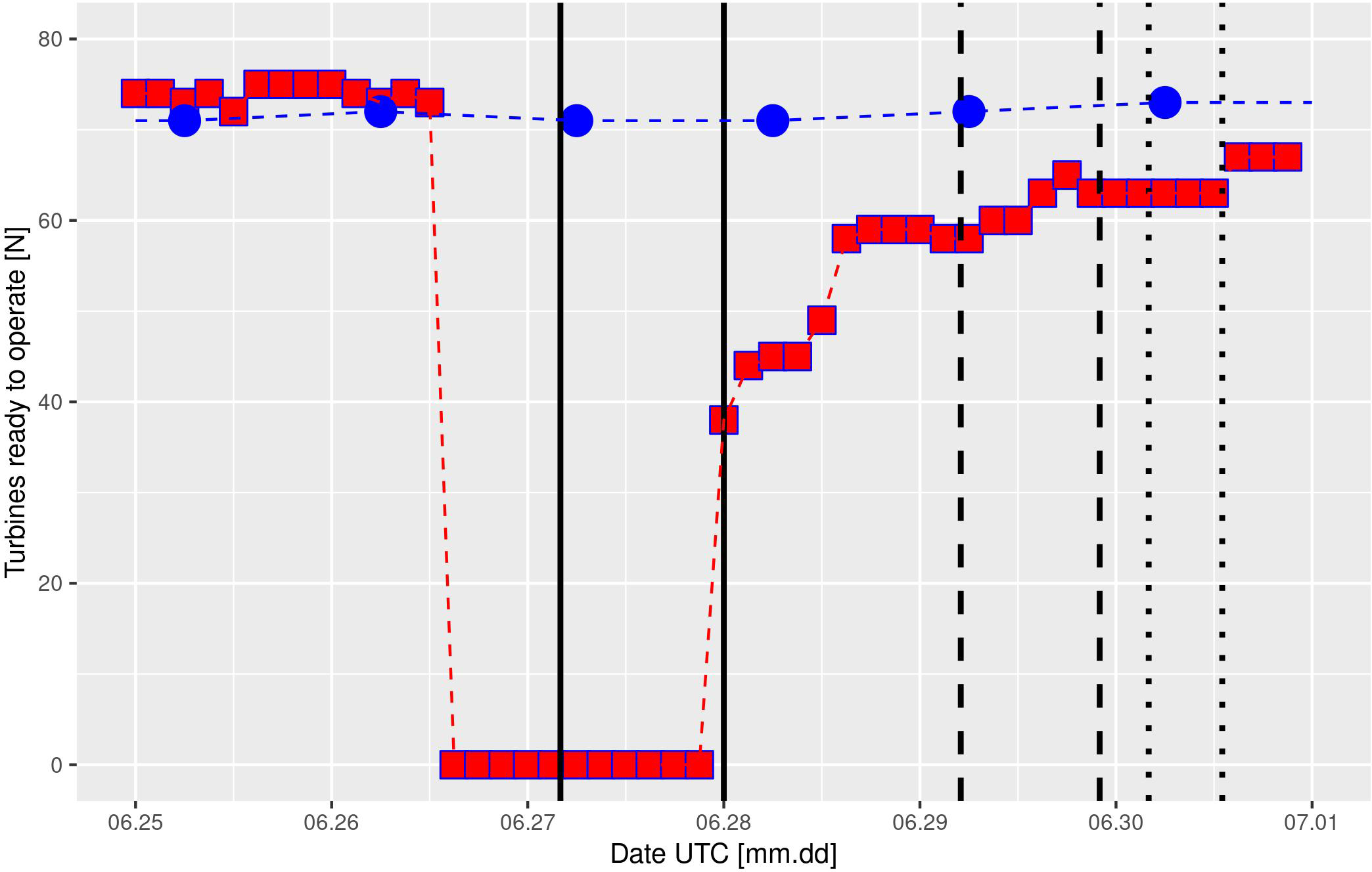
Figure 1 Numbers of wind energy turbines ready to operate during the HE466 survey period. The OWF GTI (red squares) provided data with a temporal resolution of 3 h, whereby BARD (blue circles) had a daily reporting at 5 a.m. The vertical black lines indicate the TRIAXUS ROTV field measurement periods (solid: June 27, dashed: June 29, dotted: June 30).

Satellite measurements

Moderate Resolution Imaging Spectroradiometer (MODIS) sea surface temperature (SST) data and chlorophyll-a concentrations originally obtained from the Physical Oceanography Distributed Active Archive Centre (PODAAC, ftp://podaac-ftp.jpl.nasa.gov/) were provided by the Integrated Climate Data Centre (ICDC, icdc.cen.uni-hamburg.de) University of Hamburg, Hamburg, Germany. Due to extensive cloud coverage, only data from 3 days could be analyzed (June 21, 30, July 3).

Water currents

Regional tidally and meteorologically forced currents were obtained from the baroclinic 3D ocean circulation model BSHcmod with a horizontal resolution of ~5 km and an output time step of 0.25 h (Dick et al., 2001).

Wind

Wind speed [m s^-1] and direction [°] measurements at 100-m hub height within the GTI OWF were provided by GTI with a temporal resolution of 10 min. The relative wind speed and direction at vessel height were measured with an anemometer maintained by Deutscher Wetterdienst (DWD) onboard RV Heincke. From these data, absolute wind speed and direction were calculated in real time by the onboard DShip system (Werum Software & Systems, Lüneburg, Germany).

Survey

North Sea field measurements were conducted during a summer cruise (HE466, June, 2016) with the RV Heincke (Alfred-Wegener-Institut Helmholtz-Zentrum für Polar- und Meeresforschung, 2017).

High-speed hydrographic transect measurements were conducted with a MacArtney TRIAXUS ROTV equipped with a calibrated pumped Seabird SBE 49 FastCAT CTD. Data were recorded at a frequency of 1 Hz, and the ROTV was towed at a speed of 8 knots (4.1 m s^-1) with a 3° lateral offset to lessen any disturbance from the vessel wake. The ROTV was undulating with a vertical speed of 0.1 m s^-1 from ~4 m below the sea surface to ~8 m above the sea floor. This results in vertical data spacing of 0.3 m and a horizontal resolution of around 560 m between two surface undulation turning points.

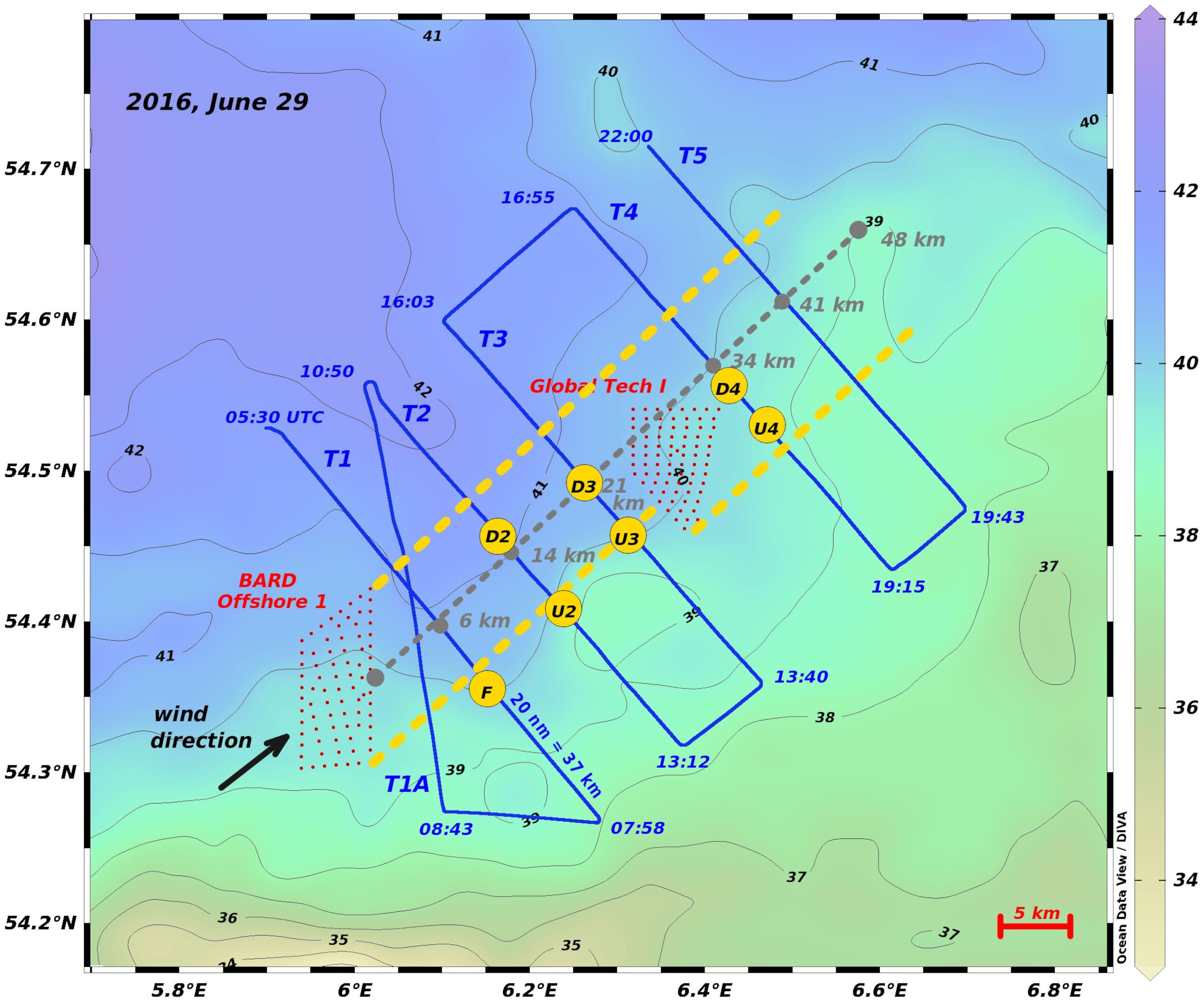
The survey started on June 27 with seven 20-nm (~37 km) TRIAXUS transects (T0–T6) which were orthogonally aligned to the initial average 220° southwesterly wind direction. The distances between the center of the transects and the center of the eastern border of BARD increased from 6 to 21 km at the leeward side of BARD and further on to 16 km at the leeward side of GTI (Figure 2). To also cover the southern leeward area of BARD, an eighth transect (T1A) was added on 29 June 2016, with a continuous approximate distance of 4 km to the eastern OWF border (Figure 6). During the third TRIAXUS measurements on June 30, only three (T1, T2, T3) transects could be covered (Figure 8).

FIGURE 2

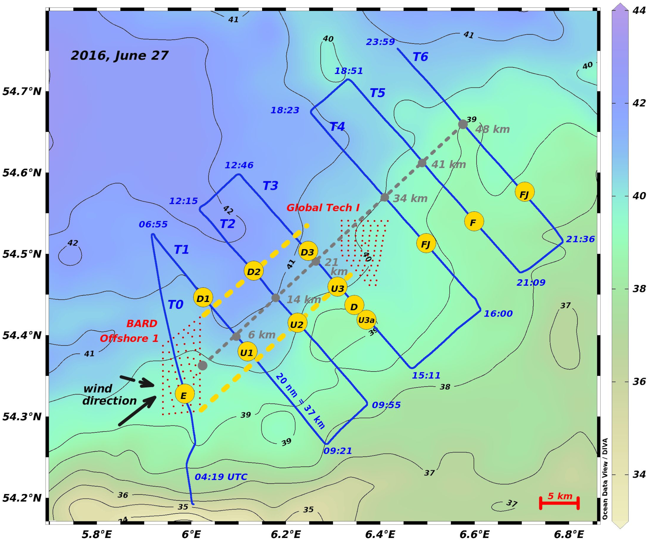
Figure 2 2016 June 27 TRIAXUS transects (blue lines, T0–T6, 04:19–23:59 UTC) in relation to the BARD and GTI wind turbines (red dots) overlaying color contours of the local bathymetry [m] of the survey area. The black arrows indicate the southwest-westerly directions in which the wind blew. The yellow-dotted lines mark the wind wake during the measurements along T0–T2. The letters “U” depict upwelling, “D” downwelling, “E” excursions of the thermocline, “F” tidal mixing front, and “FJ” frontal jet. The dashed gray line shows the distances [km] of the transects from the center of the eastern row of BARD turbines. The centers of transects T4–T6 have a ca. distance of 2, 9, and 16 km to the most eastern turbine of GTI.

Results

In summer, water temperature is affecting density more than salinity in this region. In all transects, the thermal pattern generally resembled water density; therefore, most salinity and density profiles are provided in Supplementary Material.

The average wind speed during the survey was 7.23 m s^-1 (cv: 44.7%, min: 0.7 m s^-1, max: 15.4 m s^-1) coming predominantly from the Southwest with an average direction of 221.67° (cv: 24.75%). The average southwesterly wind direction during the 24-h period preceding the first TRIAXUS tow was 234° at a speed of 8 m s^-1 (Figure 3). We hypothesize that the ambient wind conditions would produce three distinct phases (A, B, C) suitable to create wind-wake-induced upwelling/downwelling dipoles during the survey period:

FIGURE 3

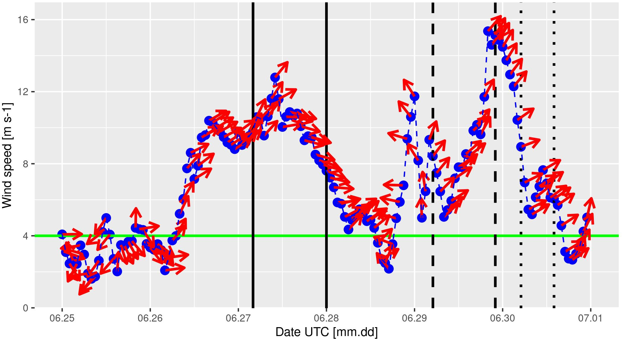
Figure 3 Average hourly wind speed [m s^-1] and direction [°] at 100-m hub height within the GTI OWF during the field measurements. Arrows point toward the direction in which the wind blew. The horizontal green line depicts the wind speed threshold of 4 [m s^-1] at which the turbines start to operate. The vertical black lines indicate the TRIAXUS ROTV field measurement periods (solid: June 27, dashed: June 29, dotted: June 30).

Phase A: Potential for an established dipole on June 27

Phase B: Potential for a developing dipole on June 29

Phase C: Potential for an eroding dipole on June 30

Phase A: potential for an established dipole on June 27

In the ~20 h preceding the ROTV measurements, the stable southwesterly wind blew with 4–5 Beaufort [~5–8 m s^-1], so that any potential upwelling/downwelling dipole should have been manifested at the leeward side of BARD (Figures 2, 3). Contrastingly, due to the complete GTI shutdown (Figure 1) we did not expect to observe a dipole at its lee side.

During the June 27 TRIAXUS transects, the wind direction changed from southwesterly 220° at the start of T0 to westerly 280° toward the end of T6 (Figures 2, 3). Wind speed at vessel height first increased from ~9 to 13 m s^-1 during T0 and T1 but decreased to ~8 m s^-1 from T3 onward (Supplementary Figures 1, 2). The 20-nm (~37-km)-long T0 transect through BARD (Figure 2) surveyed from 04:19 UTC to 06:55 UTC revealed the latitudinal transition between an intense and a weak thermally stratified water column (Figure 4). The vertical temperature difference was ~1.0°C at the shallower (36 m) southern starting position close to the border of the German Bight traffic separation scheme (TSS), which prohibited ROTV sampling, and 3.48°C at the deeper (41 m) northern end of the transect. Enhanced vertical mixing caused wiggly excursions (“E” in Figure 4) of the thermocline (~12.5°C–14.5°C) within the OWF, but a consistent upward bending (“doming effect”, Floeter et al., 2017) was missing. From the latitudinal stratification trend along T0, it was obvious that a tidal mixing front was located further south, most likely within the TSS.

FIGURE 4

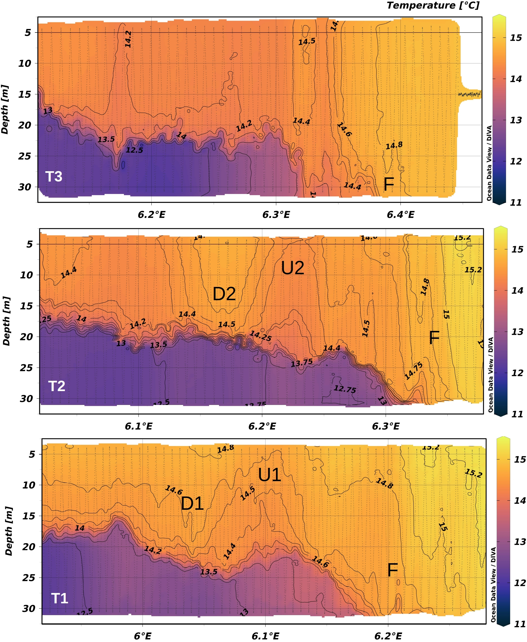
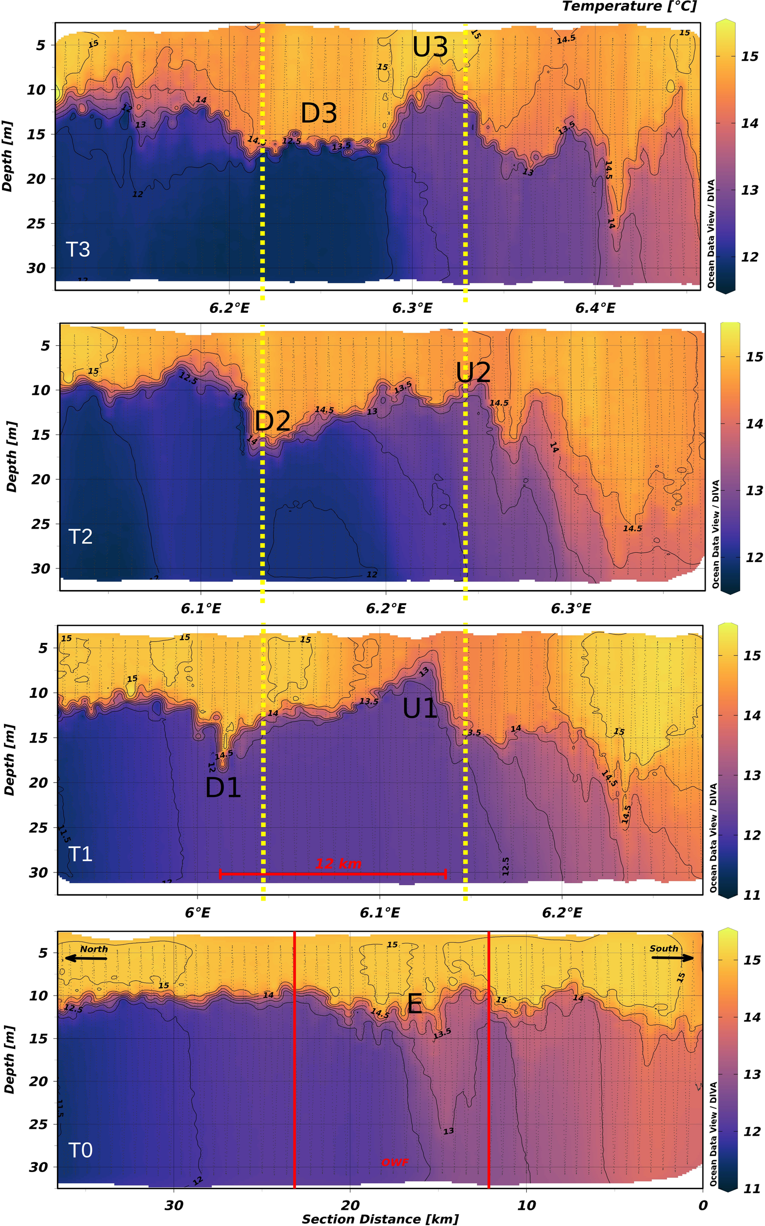
Figure 4 Water temperature color contours of transects T0–T3 on 27 June 2016. The vertical red lines mark the edges of the OWF. The yellow-dotted lines mark the wind-wake during the measurements along T0–T2. The letters “U” depict upwelling, “D” downwelling, and “E” excursions of the thermocline. The thin black lines depict the TRIAXUS undulation path. Transects T1–T3 centers have a ca. distance of 6, 14, and 21 km to the eastern border of BARD (see Figure 2).

A pronounced upwelling/downwelling dipole was observed along transect T1 at a distance of ~6 km to the eastern BARD border (Figure 2). The mixed layer depth of 12 m in the well-stratified northern transect part exhibited a downward excursion to ~19 m followed by an upward excursion to ~5 m, i.e., a vertical displacement range of ~14 m, leading to a pronounced diagonal thermocline course (Figure 4). The horizontal distance between the upwelling peak (“U1” in Figure 4) and the downwelling trough (“D1”) of the dipole eddies was ~12 km. A ~10-km-wide cooler surface patch between 6.1°E and 6.2°E exhibited a horizontal temperature difference of ~1°C in relation to the surrounding water. The surface-to-bottom temperature difference south of the upwelling eddy (~6.25°E) was >1.3°C, i.e., substantially higher than the mean 0.5°C threshold, which indicates the transition from stratified to mixed waters (Holt and Umlauf, 2008; Skogen et al., 2011; Christiansen et al., 2022). Therefore, the tidal mixing front was, as at T0, located further south and the upwelling/downwelling dipole was created by the OWF-induced wind-wake in a previously stratified water column.

Transect T2 revealed a similar dipole pattern as T1, but the downwelling trough (“D2” in Figure 4) of the dipole was larger and more pronounced than the eroded upwelling cell (“U2”), confirming the asymmetries predicted by models (Paskyabi and Fer, 2012; Ludewig, 2015). Further, a reduction in wind deficit with increasing distance from the OWF (Platis et al., 2018) leads to lower horizontal and vertical water velocities, which increases the impact of surface wind-wave-induced vertical mixing, eroding pointy upwelling signatures.

On transect T3 (Figure 2), the diagonal thermocline of T1 and T2 was replaced by an ~8-km-wide downwelling trough (“D3” in Figure 4) followed by an ~5-km broad upwelling peak (“U3”). Further south, from 6.35°E to 6.42°E a cooler patch with a horizontal temperature difference of ~0.3°C was above a feature that resembled a miniature dipole structure (“DU3a”). Around June 27 noon, the wind speed slowed down to ~10 m s^-1 and turned from southwest to west and later northwesterly directions. This led to a southeasterly shift of the expected upwelling/downwelling area as well an advection of the upper water body into this direction. Thus, the observed displacements of the hydrographic dipole signatures had been caused by these changes in the wind field, as found in modeling studies (Paskyabi and Fer, 2012; Christiansen et al., 2022).

During the June 27 survey of transects T4–T6 (Figure 2) at the lee side of the shutdown GTI, we did not expect any OWF-induced wind-wake and hence no upwelling/downwelling dipole. In the entire region leeward of GTI, we observed a horizontal salinity gradient from coastal water masses (PSU <34) to North Sea water (PSU >34, Lee, 1980; Otto et al., 1990). This led to a tidal mixing front with thermal and salinity-driven features: in the salinity profiles, frontal jets (“FJ” in Figure 5, Simpson, 1981) were visible at T4 (6.52°E) and T6 (6.7°E). As expected, upwelling/downwelling dipole signatures did not occur.

FIGURE 5

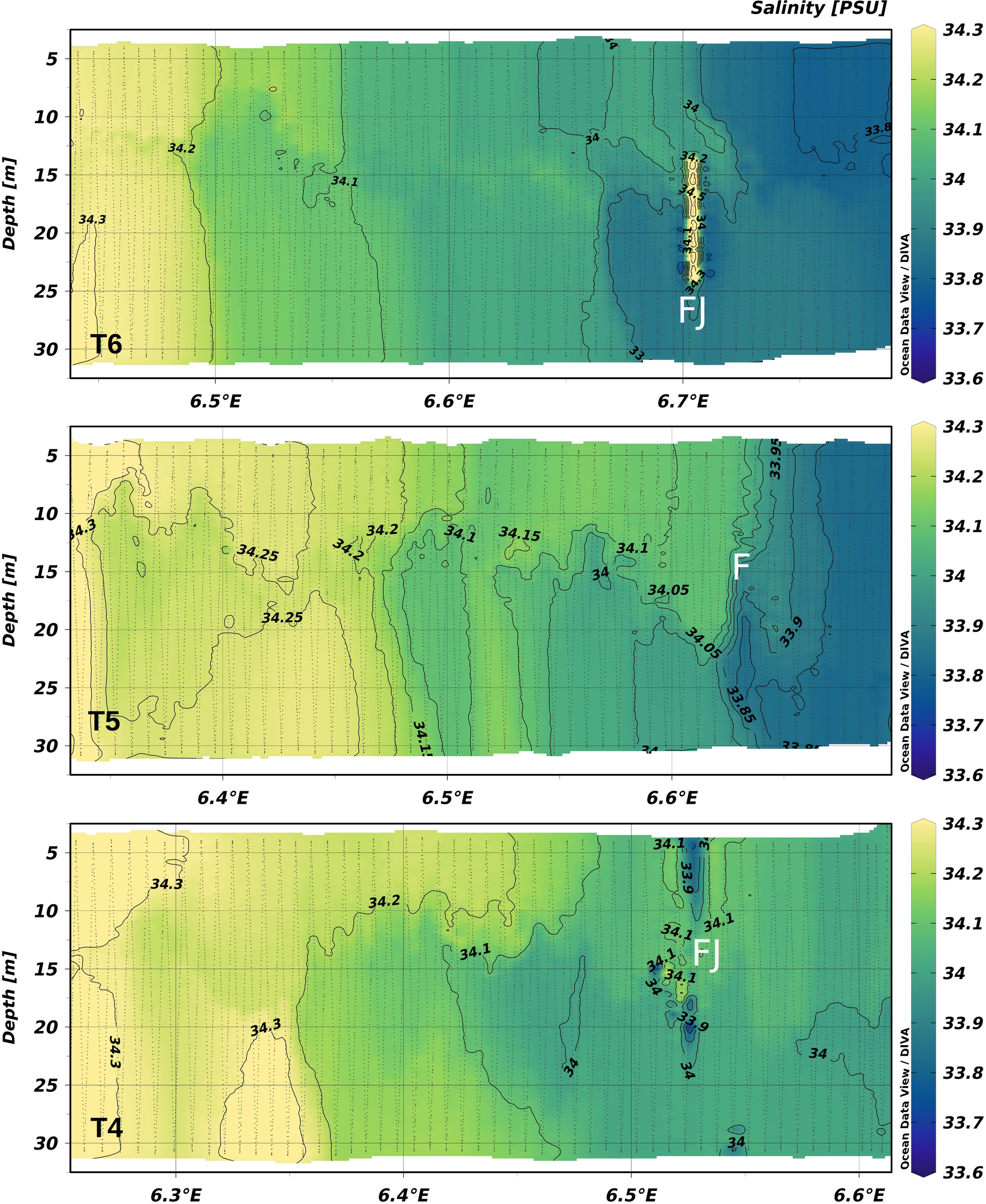
Figure 5 Salinity color contours of transects T4–T6 on 27 June 2016. The thin black lines depict the TRIAXUS undulation path. Transect T4–T6 centers have a ca. distance of 34, 41, and 48 km to the eastern border of BARD (see Figure 2). The letters “F” depict the location of a tidal mixing front, and “FJ” the occurrence of a frontal jet.

The field measurements supported our working hypothesis of an upwelling/downwelling dipole occurring leeward of BARD but not of GTI. A 12-h period with stable wind of ~10 m s^-1 generated an upwelling/downwelling dipole in a stratified water column with a vertical temperature difference of ~3°C, leading to a ~14-m vertical excursion of the thermocline, confirming previous model results (Ludewig, 2015). The spatial dimensions of the dipole observed on June 27 are depicted in Figure 4. The area affected by the dipole was ~2–3 times the size of the OWF BARD; the distance between the upwelling peak and the downwelling trough was ~12–14 km. The downwelling trough was observed at a distance of ~2 km from the eastern turbine row of BARD. The respective distance for the upwelling peak was ~6 km, most likely closer, but we did not survey transect T1A on June 27. The dipole region extended ~20 km from the OWF, close to the border of the neighboring OWF GTI (Figure 2).

Phase B: potential for a developing dipole on June 29

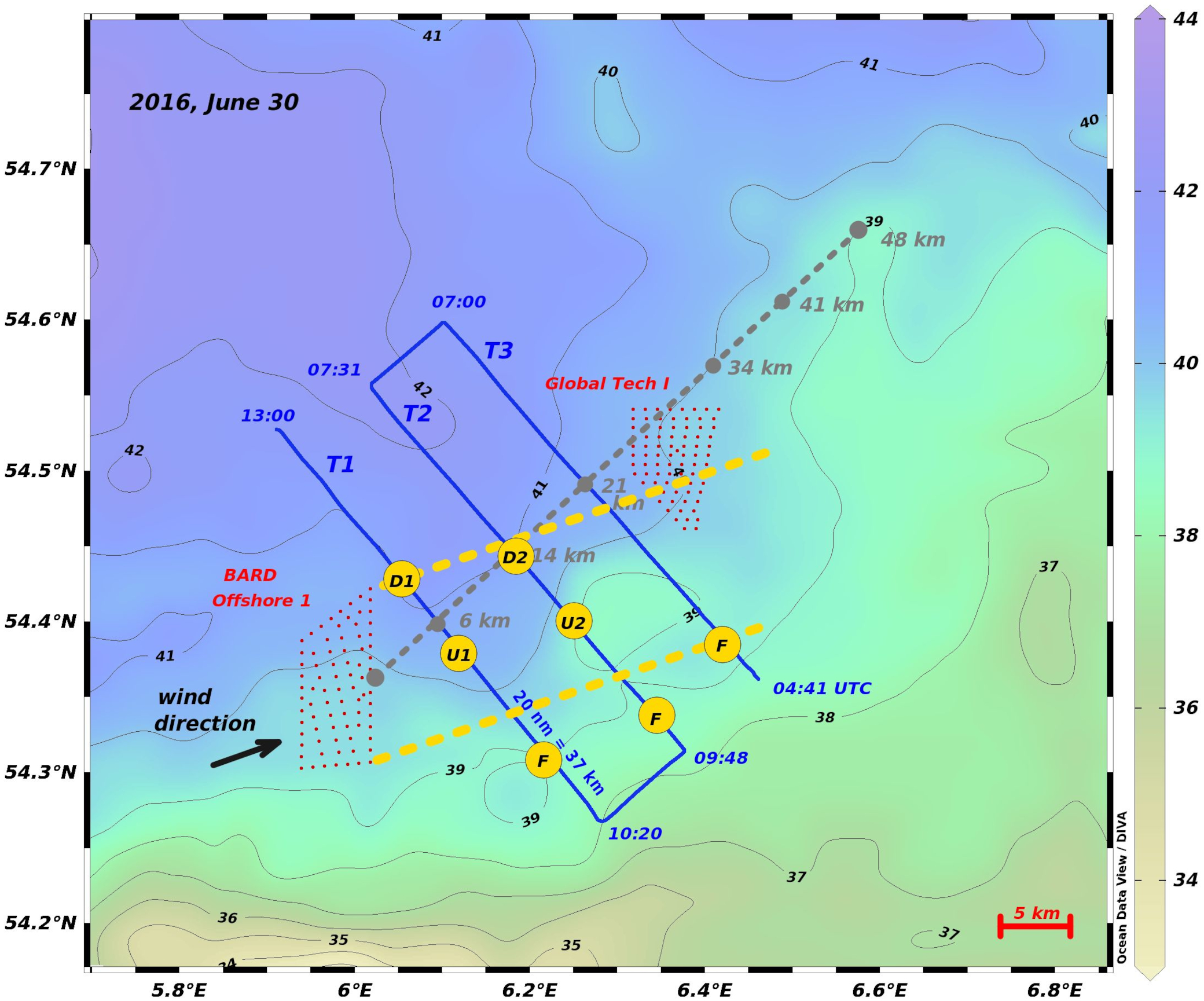
On June 28, the wind speed continued to decrease to levels below the 4-m s^-1 turbine operation threshold while its direction shifted back to Southwest. In the evening, the wind direction shifted further so that it blew for 9 h from easterly directions while increasing rapidly up to ~12 m s^-1 (6 Beaufort) and erasing the previously existing upwelling/downwelling dipole in our survey area. Subsequently, the steadily increasing southwest-westerly wind (Figure 3) should have enabled the observation of the different developmental stages of an emerging upwelling/downwelling dipole: around 5:00 on June 29, it shifted back to Southwest again, so that the TRIAXUS transects which started at 5:30 could be conducted at a quiet stable southwesterly wind direction until ca. 18:00 (223.61°, cv: 4.07%). Hereby, the wind speed at hub height within GTI was decreasing for 4 h to around 5 m s^-1 but then it increased steadily until midnight (average 7.73 m s^-1, cv: 20.7%), and from 20:00 onward it reached a speed of 15 m s^-1 (Figure 3). The resulting sea state prevented high-speed ROTV undulations as well as its recovery back onboard from 22:00 (end of T5, Figure 6) until the next morning (June 30, 4:45), so the TRIAXUS had to be towed slowly at a stable safety depth of 15 m.

FIGURE 6

Figure 6 29 June 2016 TRIAXUS transects (blue lines, T1–T5, 05:30–22:00 UTC) in relation to the BARD and GTI wind turbines (red dots) overlaying color contours of the local bathymetry [m] of the survey area. The black arrow points toward the southwesterly direction in which the wind blew. The yellow-dotted lines mark the wind wake during the measurements. The letters “U” depict upwelling, “D” downwelling, and “F” tidal mixing front. The dashed gray line shows the distances [km] of the transects from the center of the eastern row of BARD turbines. The centers of transects T4 and T5 have a ca. distance of 2 and 9 km to the most eastern turbine of GTI.

The first transect T1 started at the time when the wind direction shifted to Southwest, creating a wind-wake northeast of BARD (Figure 6). The T1 measurements took 2.5 h, a period too short to establish a dipole (Ludewig, 2015). The northern half of the transect was highly stratified, and the vertical temperature difference was about 3.1°C (Figure 7). From 6.1°E to 6.175°E, we observed an upward excursion of the thermocline, which intensified eastward and descended to the bottom. As the surface-to-bottom temperature difference at 6.25°E was small (<0.5°C), this pattern indicated a naturally occurring shelf sea tidal mixing front (“F” in Figure 7, Hill et al., 1993), e.g., as described by Munk (1993) for the southern North Sea. A “cold-belt” is a typical surface signature of upwelling at a tidal mixing front (Hill et al., 1993), which was seen as colder (~14.7°C) surface water at ~6.15°E (“CB” in Figure 7), whereas the neighboring northern (~14.9°C) and southern (~15°C) surface waters were warmer. In deviation to the classic schematic tidal mixing front circulation paradigm (Sharples and Simpson, 2019) and to the dipole-related upwelling patch on June 27, we observed an increasing trend of surface water temperature toward the coast. Under the assumption of nearly constant atmospheric heating over short distances, a shallow surface layer becomes warmer than a deeper one (Otto et al., 1990; Pohlmann, 1996).

FIGURE 7

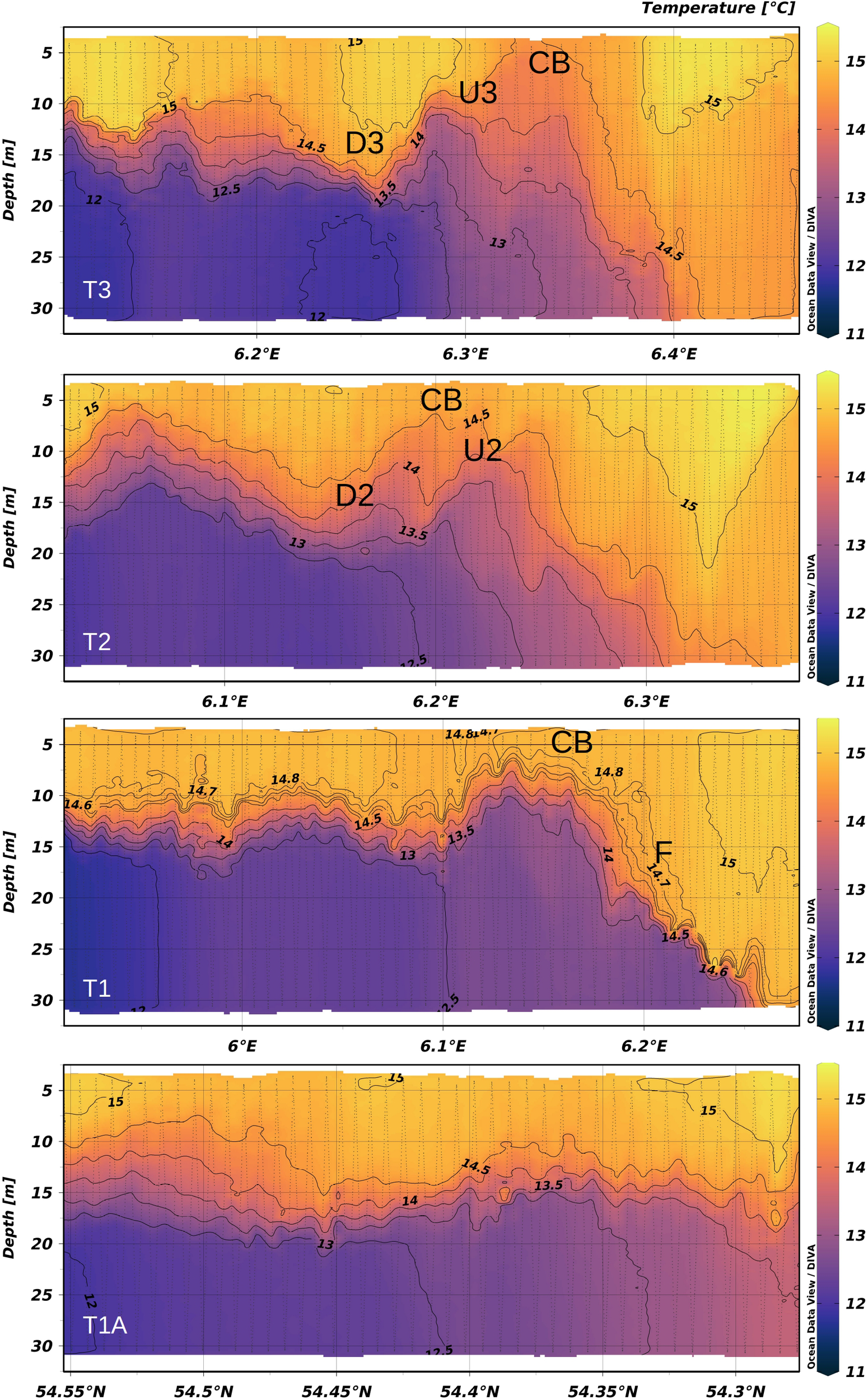
Figure 7 Water temperature color contours of transects T1A–T3 on 29 June 2016. The thin black lines depict the TRIAXUS undulation path. The letters “U” depict upwelling, “D” downwelling, and “CB” cold belt. Transect T1A–T3 centers have a ca. distance of 4, 6, 14, and 21 km to the eastern border of BARD (see Figure 6).

The second transect T1A with a distance of ~4 km to the eastern BARD border showed thermally stratified water with vertical temperature differences of 2.5°C–3°C over a broad, wiggly thermocline (Figure 7). Toward the southern end, stratification weakened (vertical difference ~1.7°C) and the horizontal surface temperature gradients were in the range of 0.1°C km^-1. Thus, it can be deduced that the frontal transition zone was further south, outside of T1A within the TSS.

Transect T2 with a distance ~14 km to the eastern BARD border revealed a frontal situation like in T1, but with less sharp vertical temperature differences (Figure 7). The “cold belt” (~14.7°C) was wider (~6.18–6.23°E, “CB” in Figure 7) compared to T1. The salinity profile (Supplementary Figure 3) revealed sharp vertical and horizontal salinity gradients, indicating a frontal jet (Simpson, 1981) next to the “cold belt” at ~6.16°E. Less dense <25.4 kg m^-3 surface water (Supplementary Figure 4) was downwelled (“D2” in Figure 7) to 12.5 m around 6.17°E. Therefore, in contrast to T1 we observed stronger upwelling (“U2” in Figure 7) and downwelling signals within the tidal mixing front, which matches with the longer (5-h) period of stable southwesterly wind.

In transect T3 (Figure 7, ~21-km distance to BARD), the “cold belt” between 6.3 and 6.4°E was sharply separated from the SML in the stratified water column (<6.3°E) and the almost mixed (vertical temperature difference <1°C) water body (>6.3°E) south of the front. Approximately 10 h after the onset of the wind-wake, we observed a diagonal shallowing of the thermocline (13.5°C–14.5°C) depth from ~20 to ~10 m between 6.25°E and 6.3°E. Both upwelling (“U3” in Figure 7) and downwelling (“D3”) regions were more defined by steeper temperature gradients.

The combined hydrography of all three transects revealed a meandering tidal front, which was generally supported by MODIS satellite-derived SST maps of the three cloud-free non-surveyed days (Supplementary Figures 5–7) and which can be explained by the local bathymetry (Figure 6): water depth is slowly but continuously decreasing along T1 and T1A, whereas the southern parts of T2 and T3 ran over a steeper depth gradient toward a small plateau (<39 m) with a trench of slightly (~0.5 m) deeper water south of it. In combination with the previously blown southeasterly wind, this led to the creation of a tidal mixing front at the southern parts of T1–T3, whereas in the region of T1A the frontal transition zone was further south. The upwelling/downwelling signatures gained intensity from T1 to T2 and T3 (Figure 7), whereby T1 was measured during the first 2.5 h after the onset of the wind-wake. The T2 hydrography was recorded 5–8 h and T3 9–11 h after the start of the atmospheric forces supposed to create an upwelling/downwelling dipole at the lee side of BARD. We interpret T1 as a naturally occurring tidal mixing front, whereas the front-related upwelling/downwelling signatures of T2 and T3 were caused by a mixture of natural bathymetric effects and the increasing anthropogenic OWF-induced wind-wake. The co-incidence of wind-wake duration, strengthened dipole signatures, and changing bathymetry along the survey route prevented the differentiation of their respective impacts.

At the lee side of the GTI transect, T4 showed a similar hydrographic characteristic as T2, a tidal mixing front with small vertical temperature differences and a weakly marked “cold belt” between 6.4°E and 6.5°E. Upwelling (“U4” in Figure 6) and downwelling (“D4”) signatures were visible, although the further increasing wind speed (>12–15 m s^-1) had already caused substantial surface waves increasing the mixed layer depth and eroding the thermocline (Supplementary Figure 8). The shallowest (water depth 38–41 m, Figure 6) transect T5 with the least steep depth gradient showed the smallest vertical temperature differences and a deep, weakly defined thermocline. Due to the high sea state, the ROTV high-speed undulations had to stop at the end of this transect.

Phase C: potential for an eroding dipole on June 30

As the wind blew from southwest with 5–15 m s^-1 for a 25-h period preceding the survey of T1, T2, and T3 at the lee side of BARD on June 30 (Figure 8), the subsequent survey period enabled the observation of possible changes in an upwelling/downwelling dipole due to wind wave-induced turbulence in the SML. The high sea state due to wind speeds up to 7 Beaufort [15 m s^-1] prevented the ROTV operation for 7 h, but then the wind speed at hub height within GTI calmed down from 10 to 6 m s^-1 t (mean: 7.05 m s^-1, cv: 22.7%, min: 5.2 m s^-1, max: 10.4 m s^-1, Figure 3) enabling high-speed TRIAXUS undulations during still stable southwesterly wind directions (238.63°, cv: 2.29%) until the end of the research cruise.

FIGURE 8

Figure 8 30 June 2016 TRIAXUS transects (blue lines, T1–T3, 04:41–13:00 UTC) in relation to the BARD and GTI wind turbines (red dots) overlaying color contours of the local bathymetry [m] of the survey area. The black arrow points toward the southwesterly direction in which the wind blew. The dashed gray line shows the distances [km] of the transects from the center of the eastern row of BARD turbines.

The resulting sea state caused intense vertical mixing, which led to a deepening of the SML from previously ~15 m (Figure 7) to ~20–25 m (Figure 9). The courses of the thermoclines exhibited neither the diagonal nor the pointy features we saw on June 27 (Figure 4). However, in T1 and T2 upwelling/downwelling signatures were visible within the SML (“U”, “D”, Figure 9). The temperature isolines at T1 indicated a tidal mixing front (“F”) at ~6.2°E, upwelling around 6.1°E (“U1”), and downwelling at ~6.05°E (“D2”), which created a warm signature in the MODIS SST measurements (Supplementary Figure 6). On T2, we saw upwelling features within the SML at ~6.2–6.25°E (“U2”) and a downwelling signature at ~6.15°E (“D2”). Transect T3 revealed rather unstructured, wiggly patterns within and above the deep thermocline.

FIGURE 9

Figure 9 Water temperature color contours of transects T1–T3 on 30 June 2016. The thin black lines depict the TRIAXUS undulation path. Transect T1–T3 centers have a ca. distance of 6, 14, and 21 km to the eastern border of BARD (see Figure 8).

The working hypothesis of an erosion of the upwelling/downwelling dipole due to increased surface-wave-induced turbulence in the SML was supported by our measurements, which again revealed the coexistence of a tidal mixing front in this region.

Discussion

Our working hypotheses of observing three different phases of an upwelling/downwelling dipole life cycle, i.e., early development, established and eroding phases, were generally confirmed. The coexistence of a tidal mixing front on June 29–30 in our investigation area prevented the observation of an undisturbed OWF wind-wake-induced development and decay of dipoles.

Wind-wakes

In situ wind and turbulence measurements of far-field OWF wakes (Platis et al., 2018) confirmed previous model- (Dörenkämper et al., 2015) and SAR-derived results (Li and Lehner, 2013; Djath et al., 2018; Djath and Schulz-Stellenfleth, 2019) that higher atmospheric stability, i.e., the absence of thermally produced turbulence, increases wake dimensions. However, we do not know the atmospheric stability during our survey.

SAR images quantifying wind-wake dimensions in a specific situation are rare, as the repeat cycle of the satellite is about 11–12 days (Platis et al., 2018), but promising (Elyouncha et al., 2021). Airborne observational data showed that in the German Bight stable atmospheric situations are most probable for southwesterly wind directions, as in our survey period, from which Platis et al. (2018) inferred that this is the most likely direction producing long wakes. However, even in unstable and neutral atmospheric situations, Platis et al. (2018); Platis et al. (2020); Platis et al. (2021) frequently observed wind-wakes with lengths between 5 and at least 35 km in our study area. Therefore, we deduced that the southwesterly wind with speeds >4 m s^-1 which prevailed during our study generated wind-wakes at the leeward regions of BARD and GTI, with lengths between 5 and ~35 km. Observations of absolute (Figure 10) and normalized (Supplementary Figure 9) wind speeds recorded at FS Heincke revealed for June 27 a clear wind deficit leeward of BARD only for T1 and T2—the transects with identified upwelling/downwelling dipoles. The wind speed deficit was ~3 m s^-1 or 30%, which is well in the range reported by Platis et al. (2018) for a similar-sized neighboring OWF. On June 29, wind-wakes with a deficit ~25% were detected at FS Heincke vessel height on transects T1, T2, T3, and T4 (Supplementary Figures 10, 11), supporting our analysis of the developing dipole. Hence, the June 27 onboard wind measurements suggest that the wind-wake had a length of ~14 km, and >20 km on June 29. On June 30, the wind-wake deficits were relatively larger (~46%) on T1 and T2 but on a lower absolute level (Supplementary Figures 12, 13).

FIGURE 10

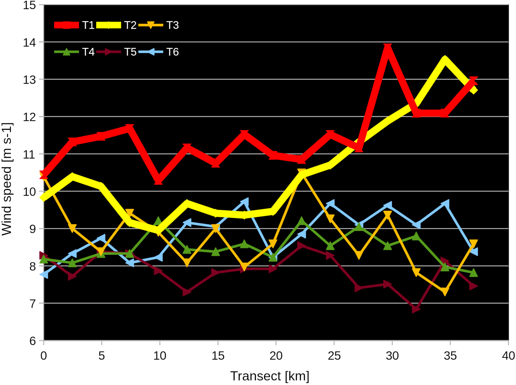
Figure 10 Absolute wind speed [m s^-1] measured at FS Heincke vessel height of transects T1–T6 on 27 June 2016. Transect T1–T3 centers have a ca. distance of 6, 14, and 21 km to the eastern border of BARD, and transect T4–T6 centers have a ca. distance of 34, 41, and 48 km to the eastern border of BARD and of 2, 9, and 16 km to the most eastern turbine of GTI (see Figure 2). Transect km 0 depicts the northern, offshore, side of the transects. The two transects T1, T2 with the identified upwelling/downwelling dipoles are depicted with bold lines.

Water currents

During the survey, maximum ambient currents in a depth of 15 m were in the order of 0.6 m s^-1, which is about one (Ludewig, 2015) to two (Christiansen et al., 2022) magnitudes higher than the mean wind-wake-induced changes in the horizontal surface water velocity field. Therefore, the spatial orientation of the tidal ellipse in relation to the direction of the wind-wake can be expected to enhance or weaken the development of an upwelling/downwelling dipole. Tidal excursions in this region have a magnitude of ~6–9 km in an east–west direction (Floeter et al., 2017), which was at an ~45° angle to the average wind-wake-induced Ekman transport during our study. Subsequently, the tidal phase can be expected to have an effect on the vertical velocities and the spatial locations of the dipoles. The BSHcmod-derived wind- and tide-driven ambient currents were similar during the comparative measurements of T1 on June 27 and 29, exhibiting a westward water movement with velocities around 0.2–0.3 m s^-1 (Figure 11). However, the tidal phase was different as on June 27 the 280° westward currents persisted for 12 h before we surveyed T1, whereas the ambient current was eastward (100°) during the 12-h period prior to the TRIAXUS measurements of T1 on June 29. A hydrodynamic modeling analysis would be needed to assess how the different tidal histories contributed to the observed dipole shapes and dynamics.

FIGURE 11

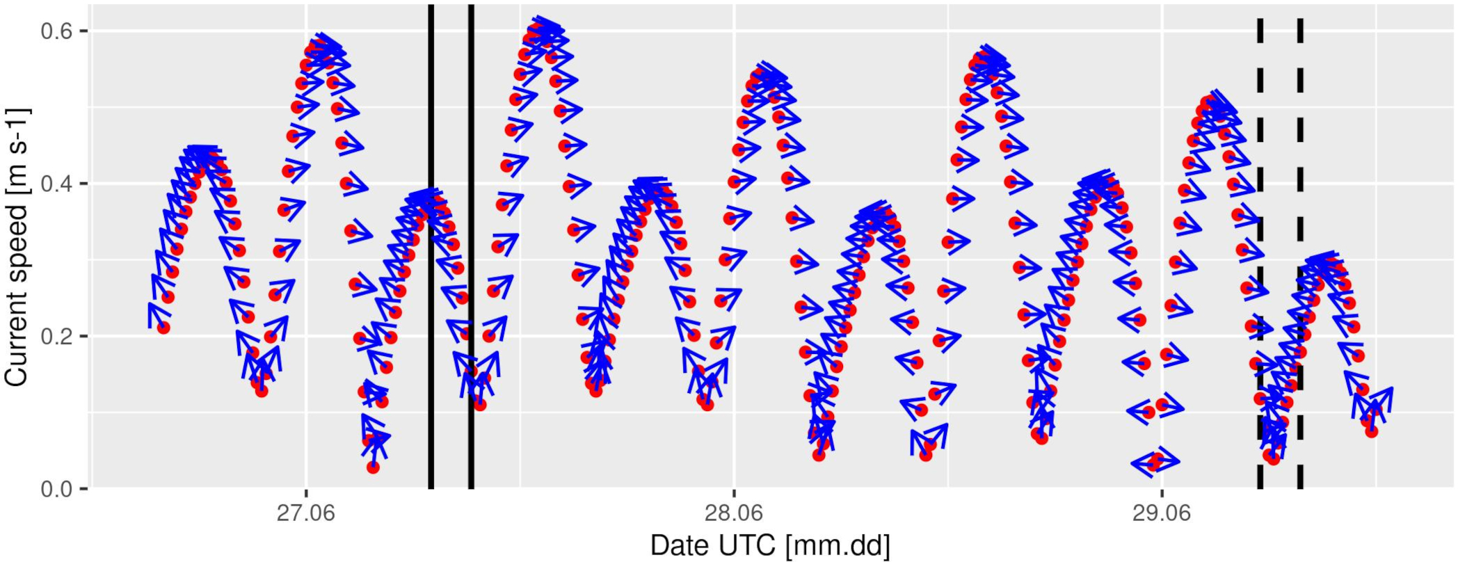
Figure 11 Time series of ambient water currents [m s^-1] in a depth of 15 m at 6.21°E 54.375°N, derived from the BSH operational circulation model. The vertical black lines indicate the T1 TRIAXUS ROTV field measurements periods (solid: June 27, dashed: June 29).

Wind-wake-induced changes in potential energy anomaly of the water column

Earlier model studies have demonstrated that OWF-induced disturbances to the wind field modulate tidal mixing front-related upwelling processes (Paskyabi, 2015) and change the upper ocean stratification pattern (Ludewig, 2015). To differentiate natural and anthropogenic effects, we calculated the potential energy anomaly of the 5–20-m envelope of the water column following the approach of Simpson (1981) by considering changes in the potential energy relative to the mixed condition [Eq. 2 in Simpson (1981)]. The calculation was based on the potential density anomalies [kg m^-3] of the transects, gridded with ODV-DIVA (Schlitzer, 2021; Troupin et al., 2012) applying a horizontal and vertical resolution of 250 m and 0.1 m.

All transects surveyed on June 27 and 29 revealed an overall north–south decrease in the potential energy anomaly, following the stratification trend from offshore to the coast (Figure 12). The trajectories of the transects with established OWF-induced upwelling/downwelling dipoles (June 27 T1, T2, and June 29 T3) were distinct from all others by showing abrupt changes in potential energy anomaly of ~4 kJ m^-3 over a short distance of ~2–4 km (Figure 12).

FIGURE 12

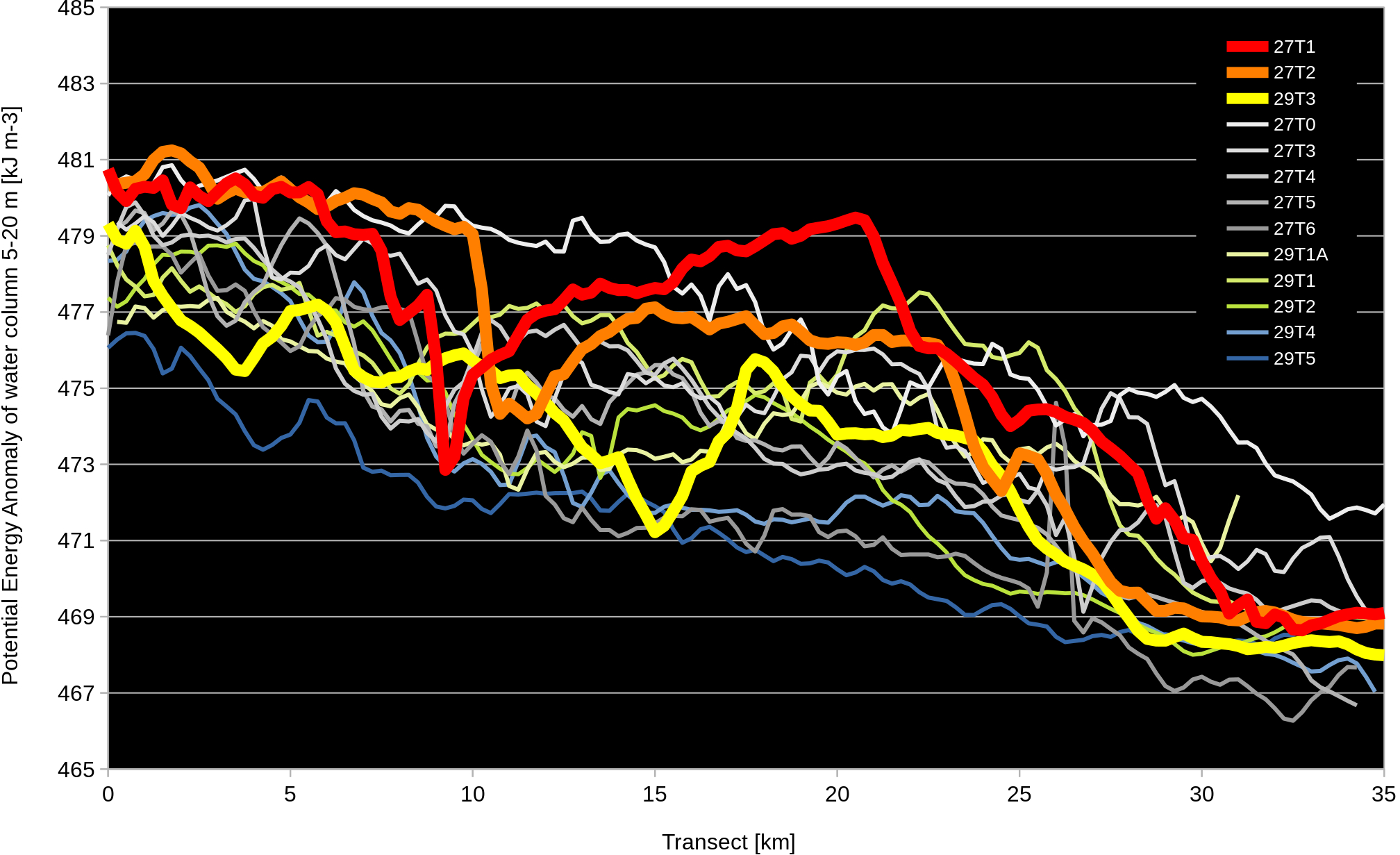
Figure 12 Potential energy anomaly [kJ m^-3] of the 5–20-m sections of the water columns along the TRIAXUS transects of June 27 and June 29. The transects start offshore at km 0 and the three clearly identified upwelling/downwelling dipoles are depicted in bold.

Characteristic signatures of the observed upwelling/downwelling dipoles

We identified two characteristic hydrographic signatures of OWF-induced dipoles:

a. Distinct changes in mixed layer depth and potential energy anomaly of the 5–20-m water column envelope over a distance <5 km

b. Diagonal excursion of the thermocline of ~10–14 m over a dipole dimension of ~10–12 km

Whether these anthropogenically induced changes in potential energy anomaly and mixed layer depth are significantly different from the corridor of natural variability awaits further investigations. The same applies to the representativity of the observed signatures.

Potential ecological consequences

In a modeling study, Christiansen et al. (2022) identified reduced vertical mixing of the upper water column due to the wind speed deficit in the OWF wake as the predominant process impacting on the pelagic environment of the German Bight. When the wind direction changes, the enhancement of stratification and shallowing of the SML is affecting varying areas. By analyzing monthly mean hydrodynamic results, Christiansen et al. (2022) concluded that OWF wind-wake-induced convergence and divergence of water masses lead to the formation of large-scale sea surface elevation dipoles, which generate structural changes in the stratification strength in the German Bight. However, because of almost constantly changing wind directions, the magnitude of the monthly averages is so low that it can hardly be distinguished from the interannual variability (Christiansen et al., 2022).

A shallowing of the nutrient-depleted summer SML (Topcu et al., 2011) brings the lower regions of the thermocline, and with it high concentrations of nutrients and phytoplankton cells (Richardson et al., 2000; Zhao et al., 2019) upward into more illuminated water depth levels. As some light for net primary production is available below the thermocline (Floeter et al., 2017), it can be expected that these phytoplankton organisms are viable and immediately increase their production.

Thus, when in a specific situation the wind direction is stable over at least ~10 h, like the ones we encountered on 2016 June 27 and 29, the shallowing of the mixed layer depth by distinct OWF wind-wakes has the potential to generate significant anthropogenic pulses of enhanced primary production at the lower spatial mesoscale (i.e., ~10–35 km). While Christiansen et al. (2022) confirmed the correlations between the sea-level dipole anomalies and changes in the vertical density and temperature distributions derived by Ludewig (2015), associated changes in the mean vertical velocity field, i.e. upwelling/downwelling dipoles were not detectable. The cause can be found in the different nature of the two main effects of OWF wind-wakes on the water column:

1) Wherever a wind-wake leads to reduced vertical mixing, the subsequent enhancement of the stratification is not reversed when the wake direction changes because the wind deficit prevails within the entire wake. Hence, the effects of this first process remain detectable in monthly average flow fields.

2) When a wind-wake directionally persists for some time, it generates an upwelling/downwelling dipole. When the wind direction changes, negative and positive vertical water velocities wipe out each other as the downwelling cell is shifted over the upwelling cell or vice versa. Hence, the effects of this second process are vanishing in monthly average flow fields.

The excursions of the thermocline due to this second wind-wake effect of upwelling/downwelling dipoles are substantially larger (~10–14 m, Figures 4, 7) than the shallowing of the mixed layer depth caused by reduced vertical mixing. Therefore, it can be expected that they generate more intense but ephemeral pulses of primary production with spatial dimensions at the lower meso-/upper submesoscale. Whether the magnitude of this anthropogenic primary production enhancement is similar to that of tidal mixing fronts awaits further investigations. At the current developmental stage of OWFs in the German Bight, their cumulative wind-wake-induced upwelling area is smaller than the tidal front region, but the potential of submesoscale features as drivers of biophysical coupling in the German Bight was already highlighted by North et al. (2016) and their location in stratified regions may make a difference.

The further fate of the manmade additional primary production, which fraction is cascading up the trophic chain (Lévy et al., 2018; Wang et al., 2018; Slavik et al., 2019; Twigg et al., 2020; Kaiser et al., 2021), how much will contribute to oxygen minimum zones (Topcu and Brockmann, 2015; Große et al., 2016; Queste et al., 2016), or the impact on fisheries resources (Methratta and Dardick, 2019; Methratta, 2020; van Berkel et al., 2020); add another level of complexity.

Data availability statement

The original contributions presented in the study are included in the article/Supplementary material. Further inquiries can be directed to the corresponding author.

Author contributions

Idea and coordination: JF. Data analysis and interpretation: JF and TP. Manuscript writing: JF, CM, and TP. TRIAXUS measurements: AH and JF. All authors contributed to the article and approved the submitted version.

Funding

The RV Heincke research cruise was supported by grant numbers AWI_HE466_00. This research did not receive any further specific grants from funding agencies in the public, commercial, or not-for-profit sectors.

Acknowledgments

We thank the captain, M. Petrikowski, and the crew of RV Heincke for their perfect support of our work. Further, we thank R. Kafemann (GTI) for the provision of the wind and turbine operation data, as well as him and C.-H. Hermanussen (BARD) for his invaluable support to obtain the permits to work inside the OWFs. Further, we thank T. Brüning (BSH) for the kind supply of BSHcmod current data and S. Kern (ICDC) for the MODIS data.

Conflict of interest

The authors declare that the research was conducted in the absence of any commercial or financial relationships that could be construed as a potential conflict of interest.

Publisher’s note

All claims expressed in this article are solely those of the authors and do not necessarily represent those of their affiliated organizations, or those of the publisher, the editors and the reviewers. Any product that may be evaluated in this article, or claim that may be made by its manufacturer, is not guaranteed or endorsed by the publisher.

Supplementary material

The Supplementary Material for this article can be found online at: https://www.frontiersin.org/articles/10.3389/fmars.2022.884943/full#supplementary-material

References

Alfred-Wegener-Institut Helmholtz-Zentrum für Polar- und Meeresforschung (2017). Research vessel HEINCKE operated by the Alfred-Wegener-Institute. J. large-scale Res. facilities 3, A120. doi: 10.17815/jlsrf-3-164

CrossRef Full Text | Google Scholar

Broström G. (2008). On the influence of large wind farms on the upper ocean circulation. J. Mar. Syst. 74, 585–591. doi: 10.1016/j.jmarsys.2008.05.001

CrossRef Full Text | Google Scholar

Carpenter J. R., Merckelbach L., Callies U., Clark S., Gaslikova L., Baschek B. (2016). Potential impacts of offshore wind farms on north Sea stratification. PLoS One 11, e0160830. doi: 10.1371/journal.pone.0160830

PubMed Abstract | CrossRef Full Text | Google Scholar

Chelton D. B., deSzoeke R. A., Schlax M. G., El Naggar K., Siwertz N. (1998). Geographical variability of the first-baroclinic rossby radius of deformation. J. Phys. Oceanogr. 28, 433–460. doi: 10.1175/1520-0485(1998)028<0433:GVOTFB>2.0.CO;2

CrossRef Full Text | Google Scholar

Christiansen N., Daewel U., Djath B., Schrum C. (2022). Emergence of large-scale hydrodynamic structures due to atmospheric offshore wind farm wakes. Front. Mar. Sci. 9. doi: 10.3389/fmars.2022.818501

PubMed Abstract | CrossRef Full Text | Google Scholar

Christiansen M. B., Hasager C. B. (2005). Wake effects of large offshore wind farms identified from satellite SAR. Remote Sens. Env. 98, 251–268. doi: 10.1016/j.rse.2005.07.009

CrossRef Full Text | Google Scholar

Christiansen M. B., Hasager C. B. (2006). Using airborne and satellite SAR for wake mapping offshore. Wind Energ. 9, 437–455. doi: 10.1002/we.196

CrossRef Full Text | Google Scholar

Dick S., Kleine E., Müller-Navarra S. H., Klein H., Komo H. (2001). The operational circulation model of BSH (BSHcmod)-model description and validation. Berichte Des. Bundesamtes für Seeschifffahrt und Hydrographie Nr 292001, 49.

Google Scholar

Djath B., Schulz-Stellenfleth J. (2019). Wind speed deficits downstream offshore wind parks? a new automised estimation technique based on satellite synthetic aperture radar data. Meteorologische Z. 28, 499–515. doi: 10.1127/metz/2019/0992

CrossRef Full Text | Google Scholar

Djath B., Schulz-Stellenfleth J., Cañadillas B. (2018). Impact of atmospheric stability on X-band and c-band synthetic aperture radar imagery of offshore windpark wakes. J. Renew. Sust. Energy 10, 43301. doi: 10.1063/1.5020437

CrossRef Full Text | Google Scholar

Dörenkämper M., Optis M., Monahan A., Steinfeld G. (2015). On the offshore advection of boundary-layer structures and the influence on offshore wind conditions. Boundary-Layer Meteorol. 155, 459–482. doi: 10.1007/s10546-015-0008-x

CrossRef Full Text | Google Scholar

Dorrell R. M., Lloyd C. J., Lincoln B. J., Rippeth T. P., Taylor J. R., Caulfield C. C.P., et al. (2022). Anthropogenic mixing in seasonally stratified shelf seas by offshore wind farm infrastructure Front. Mar. Sci. 9, 830927. doi: 10.3389/fmars.2022.830927/abstract

CrossRef Full Text | Google Scholar

Elyouncha A., Eriksson L. E. B., Broström G., Axell L., Ulander L. H. M. (2021). Joint retrieval of ocean surface wind and current vectors from satellite SAR data using a Bayesian inversion method. Remote Sens. Environ. 260, 112455. doi: 10.1016/j.rse.2021.112455

CrossRef Full Text | Google Scholar

Floeter J., van Beusekom J. E. E., Auch D., Callies U., Carpenter J., Dudeck T., et al. (2017). Pelagic effects of offshore wind farm foundations in the stratified north Sea. Prog. Oceanogr. 156, 154–173. doi: 10.1016/j.pocean.2017.07.003

CrossRef Full Text | Google Scholar

Gama J. (2016). NISTunits: Fundamental physical constants and unit conversions from NIST (R package version 1.0.1).

Google Scholar

Große F., Greenwood N., Kreus M., Lenhart H.-J., Machoczek D., Pätsch J., et al. (2016). Looking beyond stratification: a model-based analysis of the biological drivers of oxygen deficiency in the north Sea. Biogeosciences 13, 2511–2535. doi: 10.5194/bg-13-2511-2016

CrossRef Full Text | Google Scholar

Grolemund G., Wickham H. (2011). Dates and times made easy with lubridate. J. Stat. Software 40 (3), 1–25. doi: 10.18637/jss.v040.i03

CrossRef Full Text | Google Scholar

Hasager C. B., Rasmussen L., Peña A., Jensen L. E., Réthoré P.-E. (2013). Wind farm wake: The horns rev photo case. Energies. 6, 696–716. doi: 10.3390/en6020696

CrossRef Full Text | Google Scholar

Hill A. E., James I. D., Fredrick L. P., Matthews J. P., Prandle D., Simpson J. H., et al. (1993). Dynamics of tidal mixing fronts in the north sea. philosophical transactions of the royal society of London. Ser. A: Phys. Eng. Sci. 343, 431–446. doi: 10.1098/rsta.1993.0057

CrossRef Full Text | Google Scholar

Holt J., Umlauf L. (2008). Modelling the tidal mixing fronts and seasonal stratification of the northwest European continental shelf, cont. Shelf. Res. 28 (7), 887–903. doi: 10.1016/j.csr.2008.01.012

CrossRef Full Text | Google Scholar

Kaiser P., Hagen W., von Appen W.-J., Niehoff B., Hildebrandt N., Auel H. (2021). Effects of a submesoscale oceanographic filament on zooplankton dynamics in the arctic marginal ice zone. Front. Mar. Sci. 8. doi: 10.3389/fmars.2021.625395

PubMed Abstract | CrossRef Full Text | Google Scholar

Lee A. J. (1980). “North Sea: physical oceanography,” in The north-West European shelf seas: The Sea bed and the Sea in motion, vol. Vol. II . Eds. Banner F. T., Collins M. B., Massie K. S. (Amsterdam: Elsevier), 467–493.

Google Scholar

Lévy M., Franks P. J. S., Smith K. S. (2018). The role of submesoscale currents in structuring marine ecosystems. Nat. Commun. 9, 4758. doi: 10.1038/s41467-018-07059-3

PubMed Abstract | CrossRef Full Text | Google Scholar

Li X., Lehner S. (2013). Observation of TerraSAR-X for studies on offshore wind turbine wake in near and far fields. IEEE J. Sel. Top. Appl. Earth Observ. Rem. Sens. 6, 1757–1768. doi: 10.1109/JSTARS.2013.2263577

CrossRef Full Text | Google Scholar

Ludewig E. (2015). On the effect of offshore wind farms on the atmosphere and ocean dynamics (Springer International Publishing. Hamburg Studies), 162 pages. doi: 10.1007/978-3-319-08641-5

CrossRef Full Text | Google Scholar

Methratta E. T. (2020). Monitoring fisheries resources at offshore wind farms: BACI vs. BAG designs. ICES J. Mar. Sci. 77, 890–900. doi: 10.1093/icesjms/fsaa026

CrossRef Full Text | Google Scholar

Methratta E. T., Dardick W. R. (2019). Meta-analysis of finfish abundance at offshore wind farms. Rev. Fish. Sci. Aquac. 27, 242–260. doi: 10.1080/​23308249.2019.1584601

CrossRef Full Text | Google Scholar

Munk P. (1993). Differential growth of larval sprat sprattus sprattus across a tidal front in the eastern north Sea. Mar. Ecol. - Prog. Ser. 99 1-2, 17–27. doi: 10.3354/meps099017

CrossRef Full Text | Google Scholar

North R. P., Riethmüller R., Baschek B. (2016). Detecting small–scale horizontal gradients in the upper ocean using wavelet analysis. Estuar. Coast. Shelf. Sci. 180, 221–229. doi: 10.1016/j.ecss.2016.06.03

CrossRef Full Text | Google Scholar

Otto L., Zimmermann J. T. F., Furnes G. K., Mork M., Saetre R., Becker G. (1990). Review of the physical oceanography of the north Sea, neth. J. Sea Res. 26 (2–4), 161–238. doi: 10.1016/0077-7579(90)90091-T

CrossRef Full Text | Google Scholar

Paskyabi M. B. (2015). Offshore wind farm wake effect on stratification and coastal upwelling. in 12th deep Sea offshore wind R&D conference, EERA DeepWind, energy procedia Vol. Vol. 80 (Trondheim: Elsevier Ltd), 131–140. doi: 10.1016/j.egypro.2015.11.415

CrossRef Full Text | Google Scholar

Paskyabi B. M., Fer I. (2012). Upper ocean response to large wind farm effect in the presence of surface gravity waves. Energy Proc. 24, 245–254. doi: 10.1016/j.egypro.2012.06.106

CrossRef Full Text | Google Scholar

Platis A., Bange J., Bärfuss K., Cañadillas B., Hundhausen M., Djath B. (2020). Long-range modifications of the wind field by offshore wind parks? results of the project WIPAFF. Meteorologische Z. 29, 355–376. doi: 10.1127/metz/2020/1023

CrossRef Full Text | Google Scholar

Platis A., Hundhausen M., Mauz M., Siedersleben S., Lampert A., Bärfuss K. (2021). Evaluation of a simple analytical model for offshore wind farm wake recovery by in situ data and weather research and forecasting simulations. Wind Ener. 24, 212–228. doi: 10.1002/we.2568

CrossRef Full Text | Google Scholar

Platis A., Siedersleben S. K., Bange J., Lampert A., Bärfuss K., Hankers R. (2018). First in situ evidence of wakes in the far field behind offshore wind farms. Sci. Rep. 8, 2163. doi: 10.1038/s41598-018-20389-y

PubMed Abstract | CrossRef Full Text | Google Scholar

Pohlmann T. (1996). Calculating the development of the thermal vertical stratification in the north Sea with a three-dimensional baroclinic circulation model, cont. Shelf. Res. 16 (2), 163–194. doi: 10.1016/0278-4343(95)00018-V

CrossRef Full Text | Google Scholar

Queste B. Y., Fernand L., Jickells T. D., Heywood K. J., Hind A. J. (2016). Drivers of summer oxygen depletion in the central north Sea. Biogeosciences 13, 1209–1222. doi: 10.5194/bg-13-1209-2016

CrossRef Full Text | Google Scholar

R Core Team (2022). R: A language and environment for statistical computing (Vienna, Austria: R Foundation for Statistical Computing).

Google Scholar

Richardson K., Visser A. W., Bo Pedersen F. (2000). Subsurface phytoplankton blooms fuel pelagic production in the north Sea. J. Plankton Res. 22, 1663–1671. doi: 10.1093/plankt/22.9.1663

CrossRef Full Text | Google Scholar

Schlitzer R. (2021). Ocean data view, odv.awi.de. (Bremerhaven, Germany: Alfred-Wegener-Institut Helmholtz-Zentrum für Polar- und Meeresforschung).

Google Scholar

Schultze L. K. P., Merckelbach L. M., Horstmann J., Raasch S., Carpenter J. R. (2020). Increased mixing and turbulence in the wake of offshore wind farm foundations. J. Geophys. Res. Oceans 125, e2019JC015858. doi: 10.1029/2019JC015858

CrossRef Full Text | Google Scholar

Sharples J., Simpson J. H. (2019). Shelf sea and shelf slope fronts. reference module in earth systems and environmental sciences. Encyclopedia Ocean Sci. 12019, 24–34. doi: 10.1016/B978-0-12-409548-9.11457-5

CrossRef Full Text | Google Scholar

Simpson J. H. (1981). The shelf-sea fronts: implications of their existence and behaviour. Phil. Trans. R. Soc Lond. A 302, 531–546. doi: 10.1098/rsta.1981.0181

CrossRef Full Text | Google Scholar

Skogen M. D., Drinkwater K., Hjøllo S. S., Schrum C. (2011). North Sea sensitivity to atmospheric forcing. J. Mar. Syst. 85, 106–114. doi: 10.1016/j.Jmarsys.2010.12.008

CrossRef Full Text | Google Scholar

Slavik K., Lemmen C., Zhang W., Kerimoglu O., Klingbeil K., Wirtz K. W. (2019). The large-scale impact of offshore wind farm structures on pelagic primary productivity in the southern north Sea. Hydrobiologia 845, 35–53. doi: 10.1007/s10750-018-3653-5

CrossRef Full Text | Google Scholar

Thyng K. M., Greene C. A., Hetland R. D., Zimmerle H. M., DiMarco S. F. (2016). True colours of oceanography: guidelines for effective and accurate colourmap selection. Oceanography 29, 9–13. doi: 10.5670/oceanog.2016.66

CrossRef Full Text | Google Scholar

Topcu H. D., Behrendt H., Brockmann U. H., Claussen U. (2011). Natural background concentrations of nutrients in the German bight area (North Sea). Environ. Monit. Assess. 174, 361–388. doi: 10.1007/s10661-010-1463-y

PubMed Abstract | CrossRef Full Text | Google Scholar

Topcu H. D., Brockmann U. H. (2015). Seasonal oxygen depletion in the north Sea, a review. Mar. pollut. Bull. 99, 5–27. doi: 10.1016/j.marpolbul.2015.06.021

PubMed Abstract | CrossRef Full Text | Google Scholar

Troupin C., Barth A., Sirjacobs D., Ouberdous M., Brankart J.-M., Brasseur P., et al. (2012). Generation of analysis and consistent error fields using the data interpolating variational analysis (Diva). Ocean Model. 52–53, 90–101. doi: 10.1016/j.ocemod.2012.05.002

CrossRef Full Text | Google Scholar

Twigg E., Roberts S., Hofmann E. (2020). Introduction to the special issue on understanding the effects of offshore wind development on fisheries. Oceanography 33, 13–15. doi: 10.5670/oceanog.2020.401

CrossRef Full Text | Google Scholar

van Berkel J., Burchard H., Christensen A., Mortensen L. O., Svenstrup Petersen O., Thomsen F. (2020). The effects of offshore wind farms on hydrodynamics and implications for fishes. Oceanography 33, 108–117. doi: 10.5670/oceanog.2020.410

CrossRef Full Text | Google Scholar

Wang T., Yu W., Zou X., Zhang D., Li B., Wang J., et al. (2018). Zooplankton community responses and the relation to environmental factors from established offshore wind farms within the rudong coastal area of China. J. Coast. Res. 34, 843–855. doi: 10.2112/JCOASTRES-D-17-00058.1

CrossRef Full Text | Google Scholar

Wickham H. (2016). ggplot2: Elegant graphics for data analysis (New York: Springer-Verlag).

Google Scholar

Wickham H., Seidel D. (2019). Scales: Scale functions for visualization (R package version 1.1.0).

Google Scholar

Zhao C., Maerz J., Hofmeister R., Röttgers R., Wirtz K., Riethmüller R., et al. (2019). Characterizing the vertical distribution of chlorophyll a in the German bight. Cont. Shelf. Res. 175, 127–146. doi: 10.1016/j.csr.2019.01.012

CrossRef Full Text | Google Scholar