Modeling drift and fate of microplastics in the Baltic Sea

Marine plastic litter has been recognized as a growing problem and a threat to the marine environment and ecosystems, although its impacts on the marine life are still largely unknown. Marine protection and conservation actions require a detailed knowledge of the marine pathways, sources, and sinks of land-emitted plastic pollution. Model-based assessments provide a systematic way to map the occurrence of microplastics in the marine environment and to link the coastal sources to the accumulation zones in the sea. New modeling capacities have been developed, which include relevant key processes, i.e., current- and wave-induced horizontal and vertical transport, biofilm growth on the particle surface, sinking, and sedimentation. The core engine is the HIROMB-BOOS ocean circulation model, which has been set up for the Baltic Sea in a high, eddy-permitting resolution of approximately 900 m. We introduce the three-dimensional modeling tool for microplastics and demonstrate its ability to reproduce the drift pattern of microplastics in the Baltic Sea. The results of a multiyear run 2014–2019 provide the basis for an extensive validation study, which allows the evaluation of the model quality. The assessments focus on three types of microplastics, from car tires and household products, with different densities and particle sizes, which cover a broad range of land-emitted microplastic pollution. We show that the model is applicable to the task of identifying high concentration zones in the Baltic Sea and that it can be a useful tool to support the study of the environmental impacts of microplastics in the Baltic Sea. Our results suggest that microplastic concentrations in coastal regions close to major sources reach values above 0.0001 g/m3 near the surface, dependent on the buoyancy of the plastic material and the amount of discharge. The comparison with observations shows that the model is able to reproduce the average concentrations of measured microplastics in the size class of 300 μm with statistical significance, but it underestimates the very high concentrations associated either with flooding or high river-runoff events or generated by sub-mesoscale transport. The model is able to reproduce the seasonal dynamic in Latvian and Estonian waters, except for October, when the increase of modelled microplastics in the ocean is too slow. But the general spatial patterns are sufficiently well reproduced, which makes the developed model a tool sufficient for the assessment of microplastic transport and accumulation pattern.

Introduction

The marine plastic pollution of the marine environment is a severe problem that has developed into a thread since mass production started in the 1970s. Despite efforts to control the use of plastics, it is expected that global annual plastic waste production is increasing over the coming years (Kaza et al., 2018; Brandon et al., 2019; Borrelle et al., 2020). This has been recognized by the United Nations (UN), whose sustainable development goal 14.1 aims to prevent or at least significantly reduce the marine pollution by 2025, including plastics. In Europe, the Marine Strategy Framework Directive (MSFD) (Directive 2008/56/EC) (EU Commission, 2008) identified anthropogenic litter as a dominant pressure and main source of impact on coastal habitats. The MSFD sets conditions for European member states to achieve good environmental status, i.e., when the properties and quantities of marine litter do not cause harm to the marine environment (MSFD, descriptor D10).

Reaching this goal requires implementing effective legislative and management measures, as well as technological solutions to combat plastic pollution in the ocean. A deeper understanding of the sources, pathways, and sinks of plastic litter is required to effectively implement these measures (Halle et al., 2016; Geyer et al., 2017; Siegfried et al., 2017). The EU-H2020 project CLAIM develops new technologies for the prevention and in situ management of plastic pollution, including modeling capacities for microplastic transport and accumulation assessments.

Plastic debris is highly durable and tends to accumulate in the marine environment (Barnes et al., 2009). Its pathways depend on the buoyancy of the particles, which is a function of the material composition, density, and shape (Derraik, 2002). Most of the plastic items that are used in everyday applications are made from materials that are lighter than sea water and initially buoyant, when introduced to the marine environment, but some, like tire wear particles, are heavier than sea water (Parker-Jurd et al., 2021). Biofilm growth on the plastic surface is the key removal process that increases the density of initially floating plastic particles, leading eventually to sinking and sedimentation (Fischer et al., 2014; Dang and Lovell, 2015). However, it makes it also attractive for ingestion by animals such as zooplankton (Nerland et al., 2014).

The assessment presented in this study focuses on marine microplastics (<5-mm diameter) and studies the transport and accumulation in the Baltic Sea marine environment. Land-based microplastics, emitted from car tires (OSPAR et al., 2017), household products such as personal care and cosmetic products (PCCP), and fabric products, are entering the surface waters via air, surface runoff, and the effluents of wastewater treatment plants (WWTPs). The Baltic Sea is a semi-enclosed basin with a large catchment area, which is approximately four times the size of the sea (386,000 km²). Limited transport through the Danish straits, a significant runoff of 15,000 m³ s^-1 (HELCOM, 2019), and high concentrations of the population in the catchment area, of 84 million people, make the Baltic Sea vulnerable to environmental pressures from land-based sources, like plastic litter (HELCOM, 2009). Nearly half of the runoff drains into the Baltic Sea via the seven largest rivers, namely, the Neva, Vistula, Daugava, Nemunas, Kemijoki, Oder, and Göta Älv (HELCOM, 2019); all of them, except the Göta Älv, are rivers with significant microplastic loads (She et al., 2021). Estimates for the exports from the catchment to the Baltic Sea have been published, but they are either global and inadequate in resolution and coverage (Lebreton et al., 2017; Jambeck et al., 2015) or come to very different results. For this reason, the annual exports of tire wear and household microplastics to the Baltic Sea were reestimated in the Cleaning Litter by Developing and Applying Innovative Methods in European Seas (CLAIM) project, derived from national statistics, population density, and urbanization maps as well as river catchment maps (She et al., 2021). In this study, we mainly consider land-based microplastic emission to the Baltic Sea, generated by tire wear and the release of household products, based on the CLAIM source mapping results. The fragmentation and degradation of land-based macroplastic litter and microplastic inputs from paints and pellets are also important sources of marine microplastics but, for simplicity, are not included as sources in this modeling study.

Microplastic monitoring has strongly benefitted from recent research and the further development of observation techniques, as well as the intensification of the microplastic monitoring campaigns [e.g., Setälä et al. (2016); Karlsson et al. (2020); Aigars et al. (2021)]. However, the level of monitoring reached is not yet sufficient to enable a Baltic Sea–wide assessment of the spatial and temporal pattern of microplastic pollution. The studies lack spatial and temporal coverage and the regularity of annual monitoring assessments. Furthermore, a variety of monitoring and analysis methods have been used, which complicates the harmonization and integration of different data sets. The uncertainty in measured microplastic data sets have been assessed in She et al. (2022). The relative sampling errors have been found to be 40%–56% for replicate samples in the data sets.

Modeling has become an important tool for the assessment of pathways and spatiotemporal patterns of microplastics. Since the size of the particles is relatively small and their numbers are substantial, they can be treated as the concentrations of particulate matter using a Eulerian modeling framework, similar to the modeling of suspended particulate matter (SPM) (Pleskachevsky et al., 2005; Gayer et al., 2006). As such, their dynamic is affected by the baroclinic currents of the three-dimensional (3D) ocean model, horizontal and vertical mixing, the surface driving forces of the winds, and the waves and the sinking processes implemented for SPM tracers. Unlike SPM tracers, the density and sinking velocity of buoyant microplastic particles depends on the growth of a heavier biofilm shell surrounding the particles. Microplastic tracer transport studies have been carried out in the Baltic Sea by Schernewski et al. (2021) and Osinski et al. (2020) using the General Estuarine Transport Model (GETM) ocean circulation model, but their model did not include biofouling as a process to increase the density of initially floating microplastics and to remove them through sinking and sedimentation. Biofouling, sinking, and sedimentation are regarded as a major removal process for buoyant marine microplastic in the aquatic environment and must be taken into account by the model. Other modeling studies in the North Sea (e.g., Cuttat, 2018) and Mediterranean Sea (e.g., Tsiaras et al., 2021) have included the biofouling of microplastic particles. The results show that the models are capable of simulating the general spatial patterns of microplastics in the seas.

The biofouling of microplastic particles is a complex process (Fischer et al., 2014; Kooi et al., 2017). Cuttat (2018) used the Kooi biofouling parameterization for microplastic fragment transport from dolly ropes. Tsiaras et al. (2021) used a simulated concentration of specific bacteria species to parameterize the biofilm growth Cubarenko et al., 2016. In this paper, we employ a biofilm growth formulation that depends on chlorophyll-a (chl-a) concentrations in sea water to describe the strong seasonality of the biofilm growth rates obtained from fluorescence-based observations (Fischer et al., 2014). Strictly speaking, chl-a concentrations and biofilm growth activity through bacterial production are not directly linked. However, it is assumed that chl-a can be used as a proxy for the primary production, which, in turn, controls the generation of detritus. Abundant detritus in sea water can indirectly lead to the increased growth of bacteria that feed on the detritus. For this reason, we assume that chl-a concentrations can be used to determine the growth rates of biofouling in the model. An empirical biofilm growth model has been developed that uses chl-a concentrations from the Baltic Sea reanalysis product of the Copernicus Marine Environment Monitoring Service (CMEMS), provided by the ERGOM model. The model resolves the vertical dynamic by calculating the sinking velocity using the Stokes formula and by applying the sinking velocity to calculate a mass flux and associated concentration change. The velocity can be negative, for floating microplastics, in which case, the sinking term describes buoyant raising. The vertical velocity depends not only on the density and size of the combined particle and biofilm shell but also on the eddy viscosity, calculated by the model. For this reason, the particles will sink slower and remain longer in the mixed layer.

The model resolution and the ability to resolve the near coastal zone are important factors in simulating the transport of microplastic pollutants originating from land-based sources. High-resolution model simulations are required to resolve the discharge pattern realistically (Frishfelds et al., 2022). The computational efficiency of the applied ¹HBM ocean circulation and tracer transport model makes it possible to do multiyear simulations with a computationally affordable spatial horizontal resolution of approximately 926 m (≈ 0.5 nmi) in the entire Baltic Sea. This is a compromise between the available computational resources and the required resolution, which could be well below 100 m as was demonstrated by Frishfelds et al. (2022).

The wave-induced transport, mixing, and resuspension of microplastics that settle on the sediment are processes that need to be taken into account. Schernewski et al. (2021) applied wave-induced shear stress in the microplastic modeling. Tsiaras et al. (2021) included the wave-induced Stokes drift of microplastic particles. In this study, the wave-induced drift was implemented as wave-induced driving force in the momentum equation solver of the HBM ocean circulation model. This adds a non-negligible component to the transport of microplastic pollutants and might enhance long-shore transport and, in some cases, also on-shore transport, dependent on the direction of the waves in relation to the shoreline. Some of the microplastics wash ashore, but the process is more efficient for meso- and macroplastics (Hinata et al., 2017).

The objectives of our study are the 3D modeling of microplastic transport, behavior, and deposition in the Baltic Sea environment and the assessment of the spatial and temporal variability of microplastic concentration. We choose to use a Eulerian modeling framework, describing microplastics as concentrations rather than as individual particles. This allows to cover the Baltic Sea in adequate resolution and makes it easier to integrate at a later stage the microplastic model into the forecasting system of the Danish Meteorological Institute (DMI). The model results were compared with several observation data sets in the eastern Baltic Sea.

The paper is organized as follows: first, the coupled ocean circulation, wave, and microplastic transport model is described and the parameters and microplastic input data sets are introduced; next, the model results are analyzed to derive the temporal and spatial patterns of the modeled microplastic transport and accumulation in the Baltic Sea environment. The model results are compared with observations to assess its capacity to model the general dynamic of microplastics in the Baltic Sea. Finally, the results are discussed and conclusions are derived.

Materials and modeling methods

Specification of microplastic sources

Microplastics at sea cover a large range of materials and sizes, from a micrometer scale to 5 mm. This enormous range makes it necessary to identify the typical sizes and materials that can be treated in the context of drift and fate modeling. Ideally, it is possible to model a wide spectrum of microplastic particle sizes and densities. However, in this study, a simplified scenario regarding particle sizes and densities is applied. Three categories of spherical microplastic particles are selected: (1) the very small fraction with a size of 5 μm (MP1), (2) the medium- small, average fraction with a size of 42 μm (MP2) and (3) the larger fraction with a size of 300 μm (MP3). MP1 represents the tire wear microplastic particles, with a density of 1,250 kg/m³ (Kole et al., 2017). MP2 and MP3 are used to represent microplastics released from WWTPs. As shown in Vollertsen and Hansen (2017), the median value of the size of microplastic particles in the effluents of 12 Danish WWTPs is 42 μm, which is the particle size that was chosen for MP2. Microplastic particles larger than 300 μm are the ones that are usually monitored at sea. Here, we choose to include MP3 in the simulations to be able to compare model results with observations. Since household microplastics make up a large part of the microplastics released from WWTP and mainly consist of buoyant plastic materials with a lower density than seawater, a density value of 965 kg/m³ was chosen for MP2 and MP3.

The microplastic loads of tire wear particles and emissions from rivers and coastal catchments were calculated in the CLAIM project (She et al., 2021). The outcome was directly applied as an MP1 source input in the model simulations. For MP2 and MP3, the total discharge into the Baltic Sea was estimated based on an assessment of the microplastics released from WWTP. The method involves several steps. First, raw emission per capita are estimated from Danish WWTP data (Vollertsen and Hansen, 2017; Danish Environmental Protection Agency (EPA), 2015) second, a unified WWTP purification rate is applied to estimate the total emission from the Baltic Sea catchment. The total emission of the WWTPs to the Baltic Sea is estimated to be 887 tonnes per year (t/yr.) using a Danish WWTP purification rate of 99.66% (Vollertsen and Hansen, 2017), and 5,453 t/yr. by using a Finish purification rate of 97.8% (Talvitie et al., 2015). In this study, we choose to use 1,000 t/yr. microplastics entering the Baltic Sea from the WWTPs, among which, the MP2 load is 850 t/yr. and the MP3 load 150 t/yr. This distribution follows Vollertsen and Hansen (2017), who measured the size distribution of microplastics in the effluents of 12 Danish WWTPs. The results showed that 85% of microplastic particles larger than 20 μm fall in the average size class of 42 μm, represented by MP2, whereas 15% of the measured particles fall in the larger-size class, represented by MP3. The spatial distribution of MP2 and MP3 loads from rivers and costal catchment uses the spatial distribution of PCCP microplastics, which was calculated using PCCP microplastic raw emissions Magnusson and Wahlberg (2014), population density maps, river discharges, and a catchment model. Details can be found in a CLAIM report on marine plastic source mapping (She et al., 2021). The key parameters of the three microplastic categories are given in Table 1. The model used microplastic concentrations at a river inflow location (Figure 1), which are calculated from the annual discharge (t/yr.) and the annual mean fresh water runoff (m³/y) from the Swedish E-HYPE model.

TABLE 1

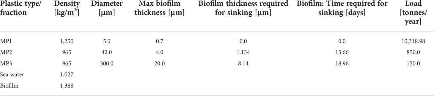
Table 1 Microplastic fractions, for tire wear microplastics MP1 and household microplastics MP2–MP3 .

FIGURE 1

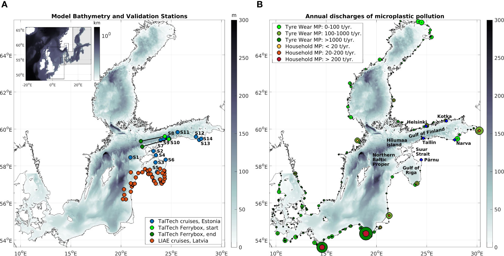
Figure 1 Model bathymetry and position of validation stations (A), as well as annual river discharges of 455 coastal sources in the Baltic Sea (B): Tire Wear MP1 microplastic loads (green) and household microplastics MP2+MP3 (red) in the units of tonnes per year.

Modeling microplastics, vertical dynamic, and removal processes: biofouling, sinking, and sedimentation

The modeling of microplastics involves the treatment of the advection and mixing processes, which are handled by the ocean circulation model HBM, as well as the treatment of vertical dynamic processes and weathering processes, i.e., biofouling, which are handled by the microplastic model implemented in the circulation model.

Plastic materials that are used in everyday life are often less dense than sea water. When they enter the marine environment, they are buoyant and float near the surface. There, they would accumulate, if weathering and removal processes would not act to reduce their concentrations. For marine microplastics, this includes the initial stages of biofouling, i.e., the settlement and the growth of algae on the particle surface, the development of a biofilm, and the removal processes of sinking and sedimentation of the particle. The time a plastic particle spends in the water column depends as much on the particle’s material characteristic, i.e., size, shape, and density, as it depends on the efficiency of the biofilm growth. The growth process is rather complex and depends on the environmental parameter. A model of proposed complexity is provided by Kooi et al. (2017). We choose to use a simpler empirical model for the biofilm thickness that would not require the tuning of too many growth parameters. The model features two tuning parameters: the maximum biofilm thickness and a time scale for growth. Initially thought to be a first approach to the problem, the simplified growth model has proven to provide stable seasonal solutions.

The implemented biofilm growth model simplifies the different stages of biofilm formation to one continuous process, focusing solely on the prediction of the floating time horizon, when, initially, lighter microplastics start sinking. The model deals with the problem in two steps: firstly, handling the growth of the biofilm thickness h_bf(x,t) , when suitable growth conditions are existent and secondly, the transport of the biofilm mass concentration using the Eulerian framework that is also employed for the microplastic concentrations. The biofilm concentration is a 3D field that is advected by the ocean currents. In its current formulation, biofouling has been implemented as a saturated growth process, using limiters for the maximum thickness h_max and the time scale of biofilm growth T_sat

$$\frac{\partial h_{bf}(x, t)}{\partial t}=\frac{h_{max}-h_{bf}(x, t)}{T_{sat}}$$

Here, bold characters indicate vectors: x being the position in space and t being the time. The density of the biofilm shell is considered to be constant and, with a value of 1,388 kg/m³, is approximately 35% larger than the density of sea water, which is 1,027 kg/m³. It is assumed that the biofilm shell surrounds the spherical particle evenly, which makes it possible to calculate the thickness of the biofilm required for sinking. The value is approximately 5.4% of the radius of the microplastic particle. Suitable parameters for the maximum biofilm thickness h_max and the growth time scale T_sat were defined empirically, on the basis of modeling experiments, but the values that have been found are in a realistic range when compared to observations (Fischer et al., 2014).

Multiyear simulations (July 2013 to December 2016) were performed to determine the set of parameters that would provide a stable overall seasonal dynamic, i.e., that would neither lead to a continuous accumulation of microplastics in the Baltic Sea nor would they lead to a complete evacuation of the Baltic Sea in summer, when biofilm growth is the strongest. Observations show that the measured concentrations during summer are non-zero. The argument for neglecting a positive trend in the entire Baltic Sea is based on the assumption that such a trend should be explained by a comparable increase in river discharges rather than by the interannual changes of the seasonal dynamic of drift and weathering processes. As the concentrations in the rivers remain constant, the amount of released microplastics is in fact a function of the river runoff, which is assumed to have no clear trend in the period of consideration. Spin-up effects play a role, but it has been found that microplastics spread very efficiently and that the 3.5-year simulation period is enough for the modeled concentrations to converge to a steady state in a weak sense, with microplastic concentrations from the sources held constant. A weakly steady state is characterized by seasonal variations, but there are no pronounced long-term trends of microplastic concentrations in the Baltic Sea environment, when the sources are kept constant. The residence time of microplastics in the ocean (not the environment) is relatively short: years rather than decades, and is determined by mass removal processes: biofilm growth, sinking, and sedimentation. The model dynamic is therefore less constrained by the initial conditions than by the boundary conditions, that is, by the coastal sources. The process with the largest uncertainty and the largest potential for model tuning is the efficiency of biofilm growth. Long-term simulations have been carried out to improve the parameterizations and to adopt the model to the harsh climate in the Northern Baltic Sea (Bay of Bothnia), where phytoplankton growth and related biofilm growth are limited to the summer seasons.

In the course of the model tuning, the time scale of biofilm growth for the large fraction of MP3 was reduced to facilitate the microplastic removal process. However, it is still in a range that compares to measurements at Kiel Fjord (54° 33’N 10° 14’E), in the south-western Baltic Sea (Fischer et al., 2014). The study involved biofilm growth measurements using optical sensors and found the cell density of diatoms or bacteriochlorophyll-a containing cells that reached the values of 10⁴ to 10⁵ cells/cm², toward the end of the measurement campaign, after 20 days. The values depend on the season: 100 10⁴ cells/cm² in October and 160 10⁴ cells/cm² in May. Assuming cells with a diameter of 10–20 μm, a surface coverage larger than 60% of hexagonally close packed cells in two layers is enough to let an MP3 particle of 300-μm diameter sink after 20 days. That is approximately the time, 18.96 days, that has been considered in the model simulations.

The model uses a combined CMEMS bio-reanalysis (BalMFC, 2019) and satellite (OC-TAC, 2019) product to determine seasonal growth conditions in the Baltic Sea. The implementation uses the local chl-a concentrations in sea water to determine the start and end of the biofilm growth season. The growth process is activated when the local chl-a concentration exceeds a critical limiter of 1.1 mg/m³, and it stops when the local concentration falls below this value. The limiter is a rather arbitrary parameter, the choice of which is justified only by its ability to represent the expected seasonal pattern of biofilm growth (Figure 2). The biofilm concentrations are advected by the flow field of the mean currents, as are the concentrations of microplastic particles to which they adhere. They can be transported out of the area of active biofilm growth but then remain inactive and do not increase their concentrations.

FIGURE 2

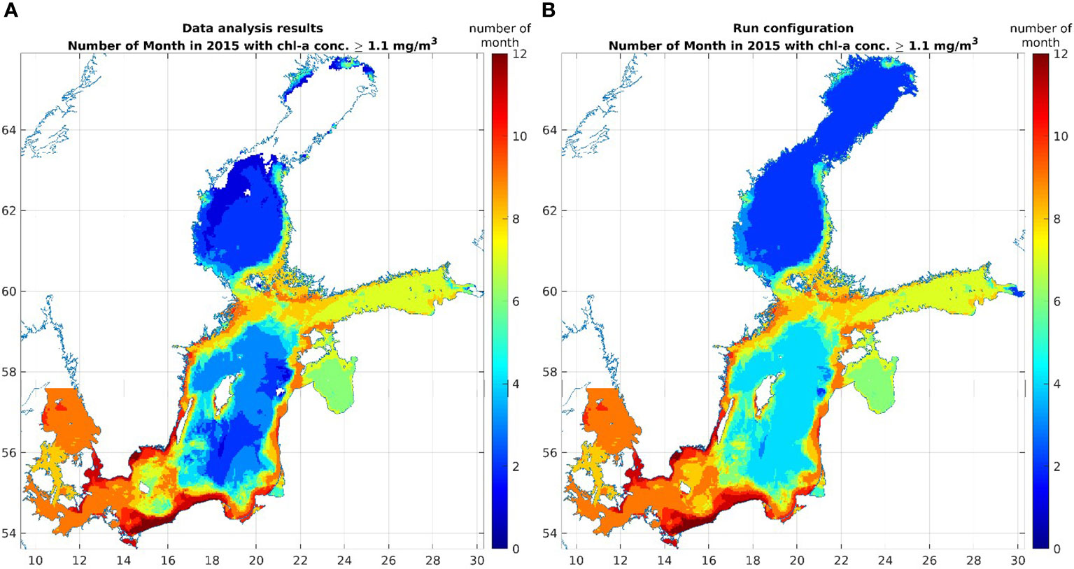
Figure 2 Seasonal pattern of biofilm growth: CMEMS bio-reanalysis (BalMFC, 2019) product (A) and combined reanalysis and satellite data (OC-TAC, 2019) product (B), with extended growth season: May–August in the entire Baltic Sea.

Biofilm growth and chl-a concentration increase through phytoplankton growth are only indirectly linked to each other. Chl-a serves as a proxy for the primary production in the ocean, which, in turn, controls the production of detritus, taken up by the bacteria involved in biofilm growth. It is assumed that seasonal changes in primary production and detritus abundancy can be used to describe the strong seasonality of biofilm growth observed in Fischer et al. (2014).

The vertical dynamic of microplastics, whether they rise to the surface or sink to the seabed, depends on their density in relation to the density of the surrounding sea water and eddy viscosity. The model applies the Stokes law for spherical particles to calculate the sinking velocity (w_sink ) as a function of the combined density of the microplastic particle and biofilm (ρ_pb ) in relation to the density of the surrounding water (ρ_w ). The model uses the eddy viscosity (μ) of the circulation model HBM, with a lower limit provided by the kinematic viscosity (ν) and fluid density (μ ≥ ν · ρ_water ).

$$w_{sink}=\frac{2}{9}\frac{{\rho }_{pb}-{\rho }_w}{\mu }g{R}^2$$

Here,R=R_p+h_b is the radius of the combined radius of the plastic particle and biofilm thickness and g is the gravitational constant. The density ρ_pb is a function of the biofilm thickness (h_b ).

$${\rho }_{pb}=\frac{R_p^3}{{\left(R_p+{\text{h}}_b\right)}^3}\left({\rho }_p-{\rho }_b\right)+{\rho }_b$$

During the floating phase, the particles accumulate in the mixed layer, from which they are removed during the sinking phase, when the particle density ρ_bf has increased sufficiently.

The vertical dynamics of sinking and rising has been implemented as a mass exchange process between vertically neighboring grid cells, which leads to a concentration change of ${\partial }_t{C}^{k+1}=\left(C^k·w_{sink}^k-C^{k+1}·w_{sink}^{k+1}\right)/h^{k+1}$ with $C^k=C^k\text{\hspace{0.17em}if\hspace{0.17em}}{w}_{sink}^k\ge 0\text{m}/\text{s}$ (in the case of sinking) and $C^k=C^{k+1}\text{\hspace{0.17em}if\hspace{0.17em}}{w}_{sink}^k<0\text{\hspace{0.17em}m}/\text{s}$(in the case of buoyant rising). Here, k is the vertical grid index, which increases with depth and h ^k+1 is the thickness of the k+1 grid cell. Mass conservation is ensured.

Sedimentation has been implemented as a sink for both microplastic particles and biofilm shells. The model uses the sinking velocity in the layer near the sediment (kb) to calculate the removal rate: ${\partial }_t{C}^{kb}=-S_{dep}=-C^{kb}·w_{sink}^{kb}/h^{kb}$ (Figure 4). Once removed from the water column, microplastic particles are permanently added to the sediment pool. Despite its limitations, the biofilm growth model is able to reproduce a seasonal dynamic for initially floating microplastics (Figure 3).

FIGURE 3

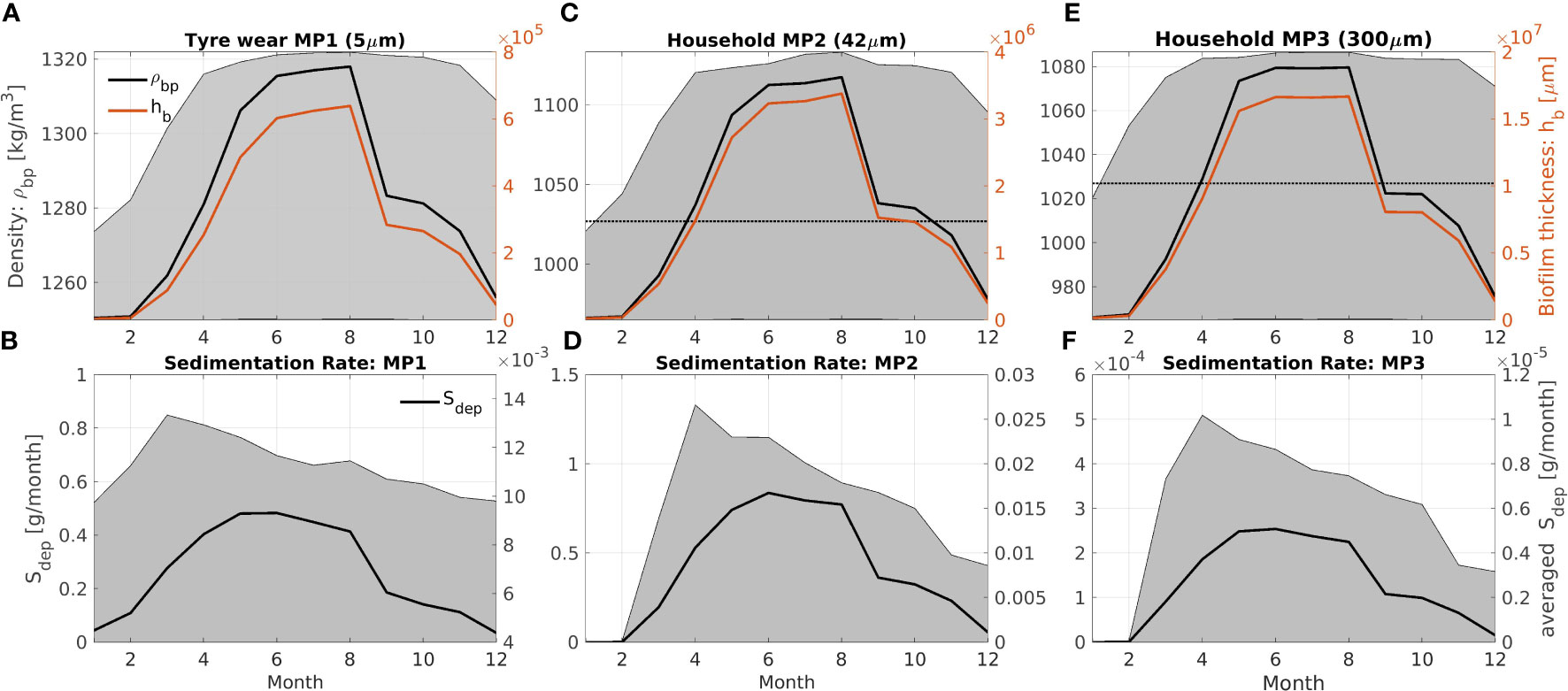
Figure 3 Monthly climatology (6-year data set: 2014–2019) of average biofilm thickness (red), density (black, panel A–C), and the range of density values (shaded areas) for tire wear microplastics MP1 (A, B) and household microplastics MP2 (C, D) and MP3 (E, F). The dotted line marks the density of sea water. Average, minimum, and maximum sedimentation rates are provided (black, panel B, D, F). Sinking velocities have been recalculated using kinematic viscosity.

Microplastic transport model

Microplastic transport simulations employ the operational ocean circulation and storm surge model HBM of the DMI. HBM is a 3D baroclinic ocean circulation and sea ice model suitable for the shelf-sea and coastal dynamics She and Murawski, 2018. It solves dynamic equations for momentum and mass, and budget equations for salinity, heat, and Eulerian tracers, on a spherical grid with a number of model levels at fixed depths in the vertical dimension. The free surface implementation allows for varying sea levels and the flooding and drying of grid cells. The horizontal advection and diffusion are modeled using a flux-corrected transport scheme. The Boussinesq approximation is applied. In the vertical direction, the model assumes hydrostatic balance and the incompressibility of sea water. Higher-order contributions to the dynamics are parameterized, following Smagorinsky (1963) in the horizontal direction and a k-ω turbulence closure scheme, which has been extended for buoyancy-affected geophysical flows in the vertical direction (Berg, 2012). The turbulence model includes a parameterization of breaking surface waves (Craig and Banner, 1994) and internal waves (Axell, 2002). Stability functions from Canuto et al. (2001) Canuto et al. (2002), Canuto et al. (2010) for the vertical eddy diffusivities of salinity, temperature, and momentum are applied. Additionally, the turbulence closure scheme considers realizability criteria (Brüning, 2020) to ensure the numerical stability of the model. HBM includes a thermodynamic and sea ice model, which describes the dynamic of free drifting ice and coastal fast ice. For more information on HBM, the reader is referred to Berg and Poulsen (2012); Poulsen et al., 2015; BalMFC group et al. (2014), and Poulsen and Berg (2012).

The HBM model was one-way coupled with the wave model WAM Cycle 4.5 (WAMDI Group, 1988; Komen et al., 1994) to improve the microplastic transport, especially in shallow waters. WAM and HBM run together as a weekly coupled system, exchanging files containing the hourly data of the wave-induced force, i.e., the divergence of the wave radiation stress, which is added to the wind-driven surface force in the HBM momentum solver. The wave surface force is a standard output of WAM Cycle 4.5. Both HBM and WAM use the same wind forcing and share the same horizontal model grid and resolution in the Baltic Sea to avoid interpolation between model grids.

The scheduling of the model system includes several sequential steps that are either performed as separate model runs of the wave and ocean circulation model or as sequential steps in the Eulerian tracer updating cycle. The first component to run is the wave model WAM, which provides hourly wave-induced drift components to the HBM model. It runs independently of HBM but uses identical meteorological forcing. The second component to run is HBM, which is reading the WAM input files every time the meteorological forcing is red. Both are provided as surface force to the momentum solver of the HBM model. After updating the 3D currents and transport, including microplastic tracers, the Eulerian tracer routine is called, which handles the growth of a biofilm on the particle surface, the associated increase in density and the resulting vertical dynamic of the microplastics. This is done every Eulerian coupler time step, i.e., every 25-s runtime. First, the model calculates the density dependent vertical velocities and the mass exchange between vertically stacked grid cells. Then, the microplastic concentrations are updated. In between the main model time steps, HBM is treating microplastics as passive tracers that are subject to advection and diffusion.

Model configuration and set-up

The HBM ocean and microplastic drift model covers the North Sea in 3-nautical mile (nmi) horizontal resolution (~5.4 km), the Wadden Sea/West Coast in 1.0 nmi (~1.8 km) and the Baltic Sea and the Transition Zone, south and east of Skagen in 0.5-nmi resolution (~900 m) (Figure 1). The setup is a further development of the DMI’s operational storm surge setup and features the same bathymetry and model configuration in the North Sea, Wadden Sea, and Transition Zone until approximately the longitude of Bornholm (14.7 °E). Further to the East and North, the setup has been extended in 0.5-nmi resolution, using publicly available bathymetry RTOPO-2 (Schaffer et al., 2016; Schaffer and Timmermann, 2016). The vertical model grid uses 122 layers in the Baltic Sea, with a varying thickness of 2 m at the surface, 1 m below the surface, and gradually increasing layer thickness of up to 50 m at layers below 100-m depth. The thickness of the lowest layer adapts to the position of the seabed. In the North Sea and Wadden Sea, the model features a thicker surface layer of 8 m, to include sea-level variations due to tides and surges, and subsurface layers of increasing thickness, of 2 m in the upper 82 m and up to 50 m below. At the open model boundaries toward the North Atlantic, between Scotland and Norway and in the English Chanel (Figure 1, inlet), the model uses tidal sea surface elevations based on 17 constituents and precalculated surges from a two-dimensional barotropic model covering the North Atlantic. The model uses boundary conditions and weather forcing from the operational forecasting system of the DMI, to ensure the good quality of the modeled ocean circulation in the Baltic Sea. HBM was forced by DMI’s high-resolution operational weather model DMI-HIRLAM until July 2018 and DMI Harmonie thereafter. The model was initialized using data from the Copernicus Marine Service CMEMS operational product, which was provided by DMI-HBM at the time. Daily freshwater runoff from the Swedish E-Hype model (Arheimer et al., 2019) is applied for 693 rivers, of which 455 are in the Baltic Sea (Figure 1).

The wave model WAM Cycle 4.5 runs in a nested sequence of three computational grids to ensure that remote swell from the North Atlantic is entering the North Sea and the Skagerrak. The large grid covers the North Atlantic from 69°W to 30°E and from 30°N to 78°N in ≈ 25-km resolution and the North Sea and Baltic Sea from 13°W to 30°E and from 47°N to 66°N in 5-km resolution. This setup provides boundary conditions for a third nested domain, which, in the operational configuration of the DMI, covers the seas around Denmark. In CLAIM, the third domain was extended eastwards and northwards, to cover the entire Baltic Sea in 900-m resolution. The full wave energy spectrum is transferred along the model interface of the WAM model boundary. The JONSWAP Spectra with a fetch of 30 km is applied to the open boundaries of the North Atlantic domain.

The Baltic Sea ocean-circulation model HBM and wave model WAM use a model grid with identical horizontal configuration and depth (Figure 1). This way, the two models can be coupled and information can be exchanged, without having to interpolate the data spatially between the different model grids. The only difference between the two model bathymetries is that WAM is using a minimum depth of 1 m, whereas there is no such limit in HBM. Another difference is related to the ice information that is used. Whereas HBM relies on its own thermodynamic and drift-ice and fast-ice dynamic routines to describe the development of the ice, the WAM model uses the satellite-derived OSTIA operational sea ice analysis product (Operational SST and Sea Ice Analysis), including OSI SAF data (Craig et al., 2011).

Modeling results analysis

Seasonal dynamic of modeled microplastics in the Baltic Sea

Baltic Sea wide assessments of microplastics pollution require model simulations on time scales that cover several years, to study offshore transport and accumulation in the deeper basins of the Baltic Sea. The here-presented assessment is based on a 6-year model simulation, covering the years 2014–2019. The model run was initialized on 1 July 2013 with realistic conditions for salinity and temperature and with microplastic concentrations from a previous 3-year run. The first half a year, until the 1st of January 2014, was used for spinning up the model. Data from this period are not taken into consideration for the model data analysis.

Figure 4 shows the seasonal dynamic of microplastics in the Baltic Sea. Highest microplastic concentrations occur near the surface and the seabed, which only make up a small fraction of the total volume of the Baltic Sea, approximately 4.3% of all grid points. The concentrations in the remaining part of the water column (95.7% of all grid points) are four-to-six times lower than the concentrations near the surface. The reason for this is that initially floating microplastic either drifts near the surface or sinks to the bottom of the sea, when biofilm growth has increased the density of the particles sufficiently enough. Figure 5 shows the modeled profile data at Bornholm Deep (station BMPK2). In the mixed layer near the surface, the microplastic concentration is quite homogeneous, at all seasons, except the biofilm-growing season: May to October, when the surface gets evacuated of MP2 and MP3 microplastics that sink to the deeper layers (Figures 4, 5: middle and lower panel). Microplastics that are heavier than sea water (Figures 4, 5: top panel) do not require the additional weight of the biofilm for sinking. Therefore, these initially sinking microplastics feature higher concentrations near the seabed, when compared with the surface concentration. The ratio of seabed-to-surface concentrations varies from 0.1 to 0.26 (large-fraction MP3, 300 μm) and from 0.15 to 0.35 (average-fraction MP2, 42 μm), to the values of 0.3 to 0.6 for the heavier but small fraction (MP1, 5 μm).

FIGURE 4

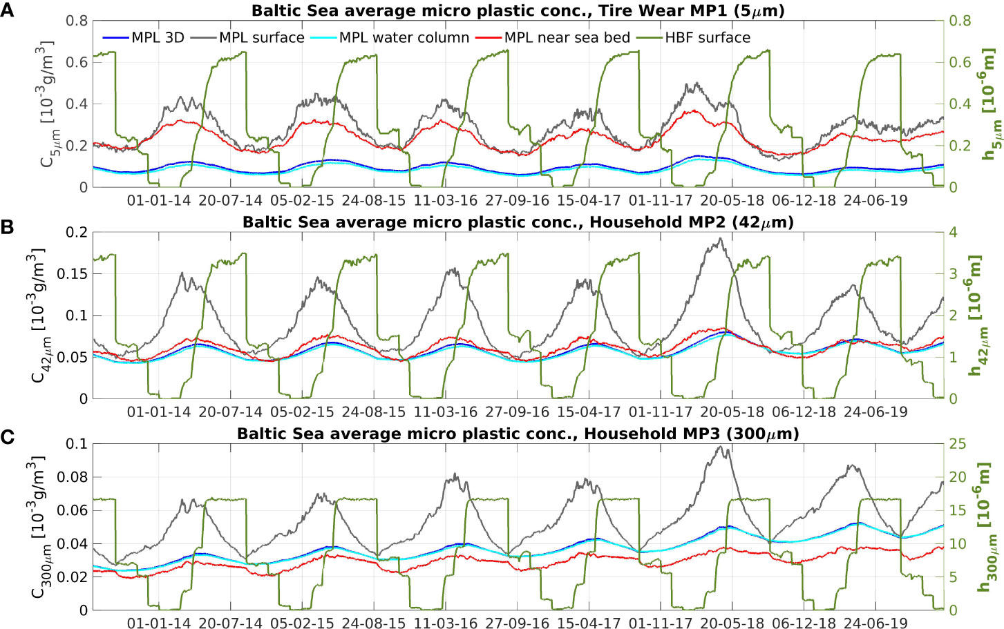
Figure 4 Time series of average microplastic concentration in the entire Baltic Sea: tire wear MP1 (A) and household microplastics MP2 (B) and MP3 (C). High concentrations exist at the sea surface (gray) and near the seabed (red), which account for 4.3% of the total number of grid points. The concentrations in the remaining part of the water column (light blue) are rather similar to the concentrations in the entire Baltic Sea (dark blue).

FIGURE 5

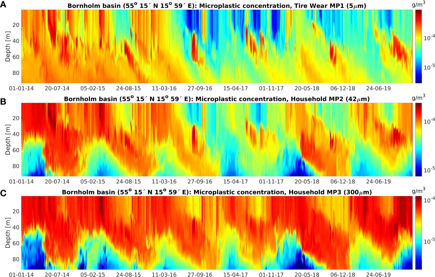
Figure 5 Profiles of microplastic concentration for tire wear MP1 (A), household microplastics MP2 (B) and MP3 (C) fragments at Bornholm deep, station BMPK2 (55° 15’ N 15° 59’ E), in the southern Baltic Sea.

The seasonal cycle of seaborne microplastic pollution is largely controlled by the river runoff and biofilm growth. The cycle starts in spring with the increase in river runoff and the related increase in microplastic discharges into the Baltic Sea. The continuous discharge and rather low activity of biofilm growth lead to a peak in the late spring or early summer season. The earliest to reach their maximum concentration are car tire particles (MP1), which are heavier than sea water and do not require biofilm growth for sinking. They reach their maximum average surface concentration of approximately 0.4–0.5 mg/m³ (1 mg/m³ = 10^-3g/m³) already in the first half of March. Initially floating particles MP2 and MP3 require more time until they develop a sufficient biofilm shell for sinking. MP2 particles reach their maximum average surface concentrations of 0.14–0.19 mg/m³ earlier, at the end of March or the beginning of April, than MP3 particles, which take longer, until latest the end of April to reach their maximum average surface concentrations 0.067–0.098 mg/m³. The peak season for microplastics near the surface ends in April for MP1, at the beginning of May for MP2, and in the middle of May for MP3, when the average surface concentration falls below the 90% level of the maximum average value. This is largely because May is the first month when biofilm growth is active in the entire region of the Baltic Sea. The Baltic Sea wide growth season ends in August, which leads to the minimum surface concentrations of MP2 and MP3 microplastics in early September.

Transport pattern of microplastics in the Baltic Sea

The mapping and visualization of microplastic pollution in the marine environment are one of the aims of drift and fate modeling. Observational data alone are too sparse, in space and time, to provide a comprehensive picture. Validated high-resolution modeling results can be used to fill the knowledge gaps and to identify the larger spatial and temporal pattern of microplastic transport.

Near-surface conditions (Figure 6) feature higher concentrations near significant coastal sources, i.e., rivers and coastal catchments. There, the surface concentrations reach the maximum values of 0.0001 g/m³ and above. Horizontal transport and mixing lead to the gradually decreasing distributions of relatively high surface concentrations near the sources (Figure 6). These surface patterns extend offshore, but they remain rather coastal. Offshore, horizontal patterns are determined by the transport of particles with the current- and wave-induced mean flow and the residence time in the upper layers of the water column. The latter is strongly affected by the efficiency of biofouling and the velocity of sinking. The small- sized but heavy-fraction MP1 (5 μm) features relatively low sinking velocity because the Stokes law depends quadratically on the particle radius. This and the relatively high amount of river discharge [roughly 10 times higher microplastic load than MP2 and MP3 together (Table 1)] lead to the pronounced pattern of MP1 in the downstream direction from the coastal sources. MP2 (42 μm) features a similar but less pronounced pattern than MP1, even though the amount of river discharge is much lower. This is due to the fact that initially floating microplastics (MP2 and 3) spread much further horizontally before the growth of a biofilm begins to affect their buoyancy, ultimately forcing them to sink to the seabed. The same is true for MP3 microplastics. However, the amount of discharged MP3 microplastics is much lower (approximately 5.6 times lower) than the discharge of MP2 microplastics. Therefore, the MP3 high-concentration pattern is much more coastal than the comparable MP2 pattern.

FIGURE 6

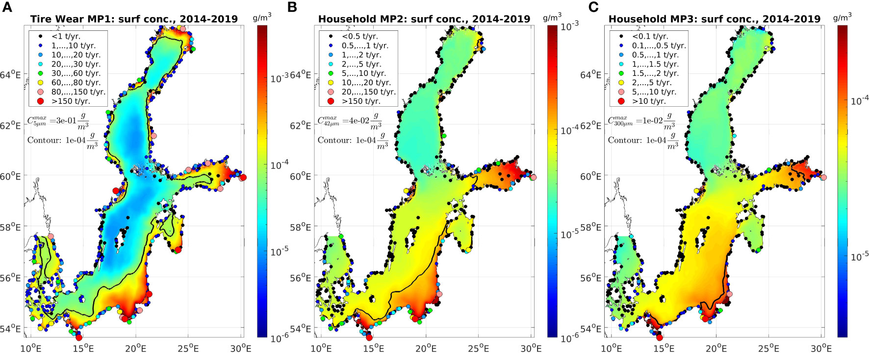
Figure 6 Surface pattern of microplastics from tire wear microplastics MP1 (A) and households microplastics MP2 (B) and MP3 (C), 6-year mean 2014–2019. Contours show the average concentrations of 10^-4 g/m³.

Oder and the Vistula are the two main riverine sources. From their estuaries in the southern Baltic Sea, the pollutants are transported away, by the generally cyclonic (counterclockwise) circulation, eastwards and northwards along the shores of Poland, Russia, Lithuania, and Latvia. At the entrance to the Bay of Riga, they mix with the plastic pollutants from the river Daugava, which enters the Baltic Sea at Riga. Further to the north and east, Neva, Baltic Sea’s largest river in terms of fresh water (2,750.14 m³/s), and the third largest in microplastic contribution, discharges its microplastic load into the Gulf of Finland (GoF). Other significant local sources are the towns of Helsinki, Kotka, Narva, and Tallin. The circulation in the GoF carries parts of the plastic pollutants out into the Baltic Proper. In the western Baltic Sea, Stockholm is a major source for microplastics. In the northern Baltic Sea, the Bay of Bothnia, Kemi, and Pori are two towns with significant river sources. That far north, biofilm growth is limited seasonally to the summer month.

Pollutant patterns near the seabed are affected by the release and transport of microplastics near the surface. High concentrations occur near the coast, in relatively shallow water and in the central Baltic Sea at Gothland Deep. While coastal patterns in shallow waters near the seabed are generated by the sinking or downwards mixing of surface concentration patterns, the generation of offshore patterns in the central Baltic Sea is mainly driven by water transport. The concentrations are therefore lower in the central Baltic Sea than they are in the coastal waters. Deeper sea transport, from the Oder banks into the Arkona Basin, around northern Bornholm and further on into the Bornholm Basin, through the Stolpe channel and into the Gothland Basin, supports the high concentration pattern in the central Baltic Sea. Tire wear microplastics MP1 follow this path more clearly, as can be seen in Figure 7 (left). The path of transport around Bornholm is visible, as is the path of the intruding high pollutions into the Gothland deep. Household microplastics MP2 follow this path somewhat after sinking. However, their larger buoyancy enables them to stay longer afloat near the surface and to spread more efficiently horizontally. Therefore, the subsurface transport pattern of submerged MP2 microplastics is not so pronounced.

FIGURE 7

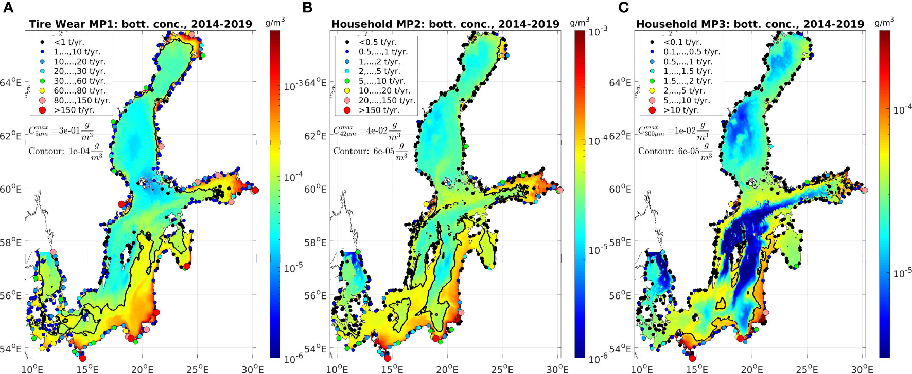
Figure 7 Near the seabed pattern of microplastics from tire wear microplastics MP1 (A) and household microplastics MP2 (B) and MP3 (C), 6 years mean 2014–2019. Contours show the average MP1 concentrations of 10^-4 g/m³ and MP2 and MP3 concentrations of 6·10^-5 g/m³.

Model quality assessment and comparison of modeled and measured particle concentrations

Model product quality assessments have been carried out to estimate the model’s skill in simulating the seasonal dynamic and spatial pattern of marine microplastic pollution. A direct comparison of the modeled and observed concentrations is difficult, as technical limitations and sampling errors lead to relatively high uncertainties in the observations, and models, on the other hand, are challenged to reproduce the observed microplastic size and density spectrum. Most of the microplastic observations in the Baltic Sea were measured by using filters with a mesh size of approximately 300 µm (She et al., 2022). Therefore, the observations include particles and fragments with a size range from 300 µm to 5 mm, made of materials with a variety of densities. The model uses a source term for the land-based discharge of a large and buoyant fraction of microplastics with a specific density of 965 kg/m³ and a size of 300 µm, added to represent measured particles with a size corresponding to the 300-µm mesh size. This makes it difficult to validate the model results by using existing observations. Therefore, we limit ourselves to the comparison of spatial and temporal patterns, focusing on the observed features and their representation by the model.

A recent study (She et al., 2022) has shown that existing observation products have several limitations thatsw4 should be taken into account when comparing model and observation data. The first is that, due to different monitoring standards used, different datasets may not be consistent. Microplastic concentration observations are more consistent in a single dataset than the multiple datasets, suggesting that using single dataset for model-observation intercomparison will reduce uncertainties comparing with blending multiple datasets. With this in mind, we select the eastern Baltic Sea as the study area, which has best spatiotemporal coverage of microplastic observations. The second is that the mean relative sampling error of microplastic samples is approximately 40%–56%, which means that even taking replicate samples they still show high uncertainty. The lack of surface flow correction will lead to additional 12% uncertainties. In addition, there also exist errors in analysis methods that can be high in some occasions (She et al., 2022). These results suggest that individual observations can have large uncertainties and may not be suitable for direct comparison with model data. With this in mind, we try to avoid a direct comparison of individual observations but focus on intercomparing some aggregated indexes, e.g., temporal mean for subregions and the mean values of individual cruises. It was also identified in She et al. (2022) that microplastic fiber observations may not be reliable due to its potential leakage from the filters; therefore, are not good for microplastic model validation. For this reason, we have focused the assessment on fragments alone.

Microplastic observations provide information about the number of particles per sampled volume of water, i.e., numerical particle concentration, whereas the outcomes of model simulations are microplastic mass concentrations in a unit of mass per unit volume. The conversion from the measured particle concentrations to modeled mass concentrations is unfortunately not trivial because the size of the observed particles is not available from the observation database. The only information of the size range is provided by the mesh size: 330–333 µm and the microplastic size limit of 5 mm. This provides a rather large uncertainty. We have chosen to use a standard particle size of 500 µm when converting the modeled mass concentrations to the numerical particle concentrations so that the modeled numerical particle concentration is at a similar concentration level as in the observation data. It is also reasonable to assume that the average particle size in the observation database is larger than the mesh size (330–333 µm), which only provides a minimum size limit.

Data sets

The model-observation intercomparison exercise uses data sources from (a) HELCOM and available publications, as well as (b) cruise data (Manta Net observations) that have been collected during the CLAIM project. Measurements using pumps have been removed from data sets. The model evaluation is limited by the availability of observation data sets, which makes it difficult to assess the model quality on spatial and temporal scales separately. We have therefore decided to do spatiotemporal assessments of the model–observation correlation coefficient by including all available data sets, sorted according to location. Furthermore, the best coverage of the data set is in the GoF and Estonian waters. We have therefore limited the assessment of correlation pattern to the GoF and the seas around Estonia.

The model–observation intercomparison area covers Latvia and Estonian waters in the GoF, Gulf of Riga (GoR), and open Eastern Baltic Sea. The GoF and GoR are connected by the Suur Strait (Figure 1). Three observation datasets are used: (a) a trawl dataset in Estonian waters made by the Tallin Technical University (TalTech; Mishra et al., 2022), (b) a trawl dataset in Latvian waters made by the Latvian Institute of Aquaculture and Ecology (LIAE; Aigars et al., 2021), and (c) a ferrybox dataset in southwestern GoF, provided by the CLAIM project. The spatial distribution of the stations is displayed in Figure 1.

Latvian institute of aquaculture and ecology data

This data set includes 43 samples from six cruises in June–September 2018 (Figures 1, 9). The data, covering southern GoR and eastern Baltic Latvian coastal and offshore waters, are publicly available from Aigars et al. (2021). The samples were collected by using manta trawling with a mesh size of 300 µm and analyzed with the Fourier-transform infrared spectroscopy (FTIR) method. Most of the stations only have one sample. More details of this data set can be obtained from Aigars et al. (2021).

TalTech data

This data set was collected during April 2016–August 2020, mainly during the summer half-year. The monitoring was carried out using the research vessel Salme with a manta trawl with a mesh size of 330 µm in a geographical area (20.9–28.0°E, 57.6–59.9°N) including southern GoF, Suur Strait, northern GoR, and Northern Baltic Proper (NBP) (Figure 1). In total, there are 14 stations and 121 valid samples (Table 2), which were analyzed with a visual and burning needle examination. More details on the TalTech dataset can be found in Mishra et al. (2022).

TABLE 2

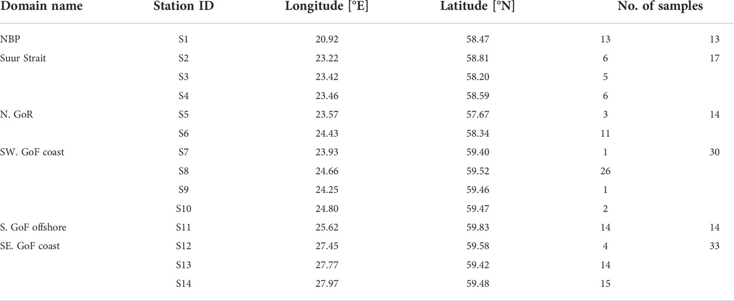
Table 2 The coverage and number of samples in the TalTech data set during April 2016–August 2020.

Some preprocessing of the data has been made to improve the homogeneity of the TalTech data. For 2017, three replicate samples are collected at each of the seven stations. The replicate samples are averaged before they are used in the analysis. Hence, the total number of TalTech reprocessed data is 106. In order to reduce the uncertainty in individual observations, we decided to group the 14 stations into six subregions, i.e., NBP, Suur Strait, northern GoR, southwestern GoF coastal waters, southern GoF offshore, and southeastern GoF coastal water (Table 2). The sample size per subregion ranges from 13 to 33, which makes the temporal mean of the subregions more representable.

Ferrybox data: CLAIM ferrybox data have been collected during two cruises in Estonian waters near the entrance to the GoF. All the cruises started in Tallinn, but only the earlier cruise stayed in coastal waters, going from Tallinn to the most western point of Hiiumaa island (Figure 1). The later cruises started in Tallinn but went to locations further offshore before starting the monitoring. The monitoring periods, 30.11.2020–01.12.2020 and 30.06.2021–01.07.2021, are not covered by the time period of the model data (2014–2019). Therefore, the model data have been extracted from a monthly mean climatology that has been derived from the 6-year model data set. It is expected that this adds to the model errors as the model data set does not reflect the metocean conditions that were present at the time of the observation.

The comparison between the model and ferrybox data is particular with regard to the fact that the duration and spatial extent of the cruise have to be taken into consideration. The model data were therefore averaged along the estimated track of the cruise, which has been estimated from the start and end location of the cruise. We extracted model data at three points, the start and end location of the monitoring, as well as a location in between. These values were averaged and compared to the observations, which represent the average state of microplastics for the entire cruise.

Spatiotemporal correlation analysis

Correlation analysis studies the degree to which a tendency in one data set (model data) is statistically related to a tendency in another data set (observations). Since the analyzed data sets are spatially and temporally distributed, these tendencies can relate to a spatial pattern: coastal-to-offshore transport, or a temporal pattern, representing the annual, seasonal, or diurnal variability in the data set. The correlation analysis is conducted for LIAE and TalTech datasets separately, using observed and modeled particle concentrations. The model concentrations have been derived from the outputted mass concentrations using an average particle size of 500 μm to calculate the mass of each particle.

The scatter diagram of modeled and observed values is shown in Figure 8. For the LIAE data, most of the observed microplastic fragment concentrations are lower than 0.4 pcs/m³ while the model concentrations are higher than 0.3 pcs/m³ and show less variability. Further analysis suggests that there is no significant correlation between the two data sets. This may be attributed to the lack of temporal sampling at the LIAE stations and a large uncertainty of individual samples due to sampling errors and missing surface flow correction. Surface flow correction accounts for the currents and wave-induced flow of water through the measuring device that is not accounted for when only the towing speed is considered in the calculation of the water volume.

FIGURE 8

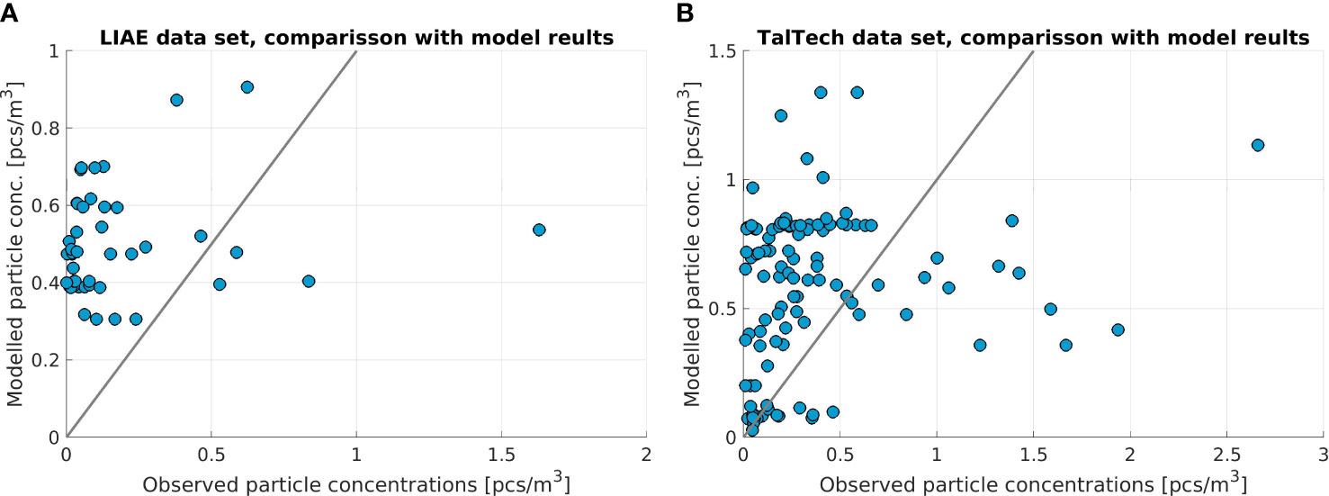
Figure 8 Scatter plot, i.e., a model–observation diagram, for the LIAE data set in June–September 2018 (A) and TalTech data set in 2016–2020 (B).

For the TalTech data, the observed concentration of microplastic fragments varies between 0 and 3.0 pcs/m³ while the simulated data ranges from 0 to 1.3 pcs/m³. The percentage of samples with concentrations of microplastic fragments below 1 pcs/m³ is 92%. Since the sampling period of the TalTech data covers the years 2016–2020, the correlation analysis represents the spatial and temporal relationship between the model and observed microplastic fragment concentration. The results show a correlation coefficient of 0.269, with a P-value of 0.005. If the data with observed microplastic concentrations larger than 1 pcs/m³ are removed, the correlation coefficient increases to 0.355 and the P-value decreases to 0.00035. Both correlations are significant at p< 0.01.

Spatial pattern

Spatial pattern analysis provides insight about the quality of the model and its ability to reproduce spatial features of the observed microplastic distribution. The spatial distribution of the mean microplastic fragment concentration from the model and observations and bias and centered Root Mean Square Error (cRMSE) are displayed in Figure 9. It should be noted that all three datasets are used, although the number of samples are quite different. The concentration values at TalTech stations represent a temporal mean, while those at LIAE stations and from the ferrybox contain both spatial and temporal (month by month) variability (Figs. 9A and 9B).

FIGURE 9

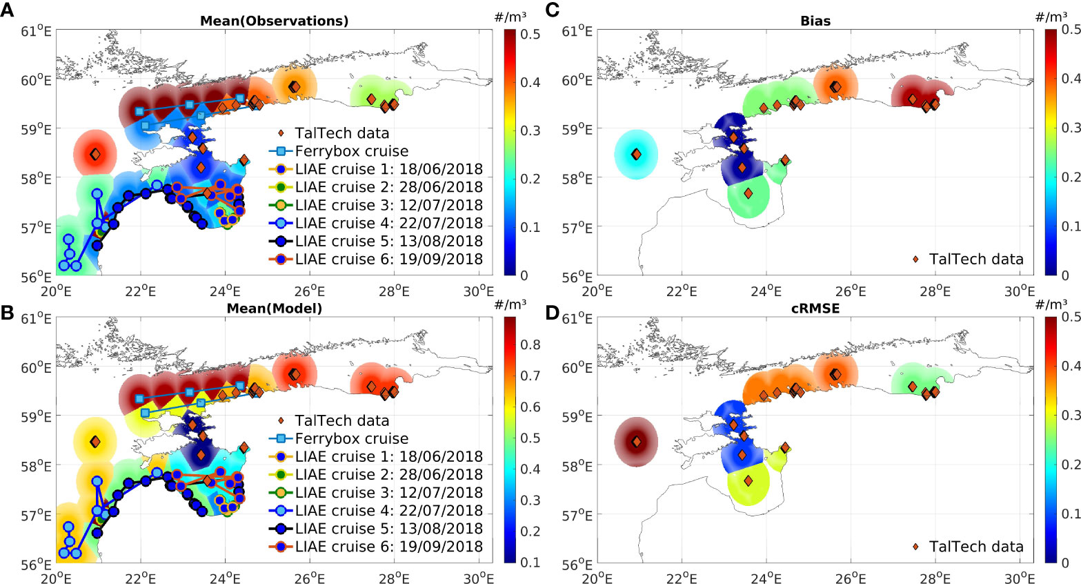
Figure 9 Left: Mean microplastic particle concentrations: Observed pattern (A) and modeled pattern (B). Right: Model error statistics for TalTech data sets: Bias (C) and centered RMSE (D). LIAE cruise data have been added in (A) and (B) but have not been used in the error analysis because of low statistical significance.

Figure 9A shows the observed spatial distribution of microplastic fragment concentration in the eastern Baltic Sea. In the Estonian waters, microplastic fragment concentrations are the highest in the NBP and southwestern GoF and the lowest in the Suur Strait and northern GoR. Ferrybox data show that, near the entrance of the GoF, the offshore winter concentration is higher than the coastal summer concentration. LIAE cruise data show higher values in western Latvian offshore, the entrance of GoR, and areas downstream the Daugava estuary. Near cities and coastal sources, at Tallin, Narva, and Riga (Daugava), the microplastic concentrations are consistently higher than the concentrations further offshore, except in areas that are affected by microplastic transport: the offshore locations in the GoF, for example.

The simulated spatial distribution (Figure 9B) also shows high concentrations in the NBP and southwestern GoF and low concentrations in the Suur Strait and northern GoR. However, the model data have the highest concentration in southeastern GoF, mainly affected by the Neva and Narva. The model data show a similar pattern when compared with ferrybox data and LIAE data. The comparison of spatial distribution in TalTech data can be further illustrated by using the subregional mean concentration (Figure 10). The analysis for the subregions shows that the NBP is the area with the highest mean observed concentration (0.42 pcs/m³), whereas the lowest observed concentrations are found in Suur Strait (0.08 pcs/m³). In the NE-GoR, including a station near Pärnu, the concentrations increase to 0.17 pcs/m³. Further to the North, in the GoF, the observed concentrations increase toward the Tallin coast (0.39 pcs/m³) and offshore (0.37 pcs/m³) and decrease toward Narva (SE-GoF) (0.27 pcs/m³). The model is able to reproduce the general features of the observed spatial pattern except for observed lows in the Narva area. The correlation between the averaged model and observation data sets for subregions is 0.81, with a P-value 0.051. In the GoF, the west-eastern trend is reversed, showing an increase of modeled concentrations from 0.64 pcs/m³ at Tallin coast to 0.75 pcs/m³ at Tallin offshore and Narva (SE-GoF). To analyze this further, the model bias and the cRMSE, the root-mean-square error (RMSE) of the debiased data sets, are analyzed in more detail (Figs. 9C and 9D). cRMSE represents the errors originating from the sample spread of model-observation differences and is therefore affected by individual sampling and model errors, especially when the sample size is small. Model error statistics, in particular the model biases, are affected by the conversion from modeled mass concentrations to measured particle concentrations.

FIGURE 10

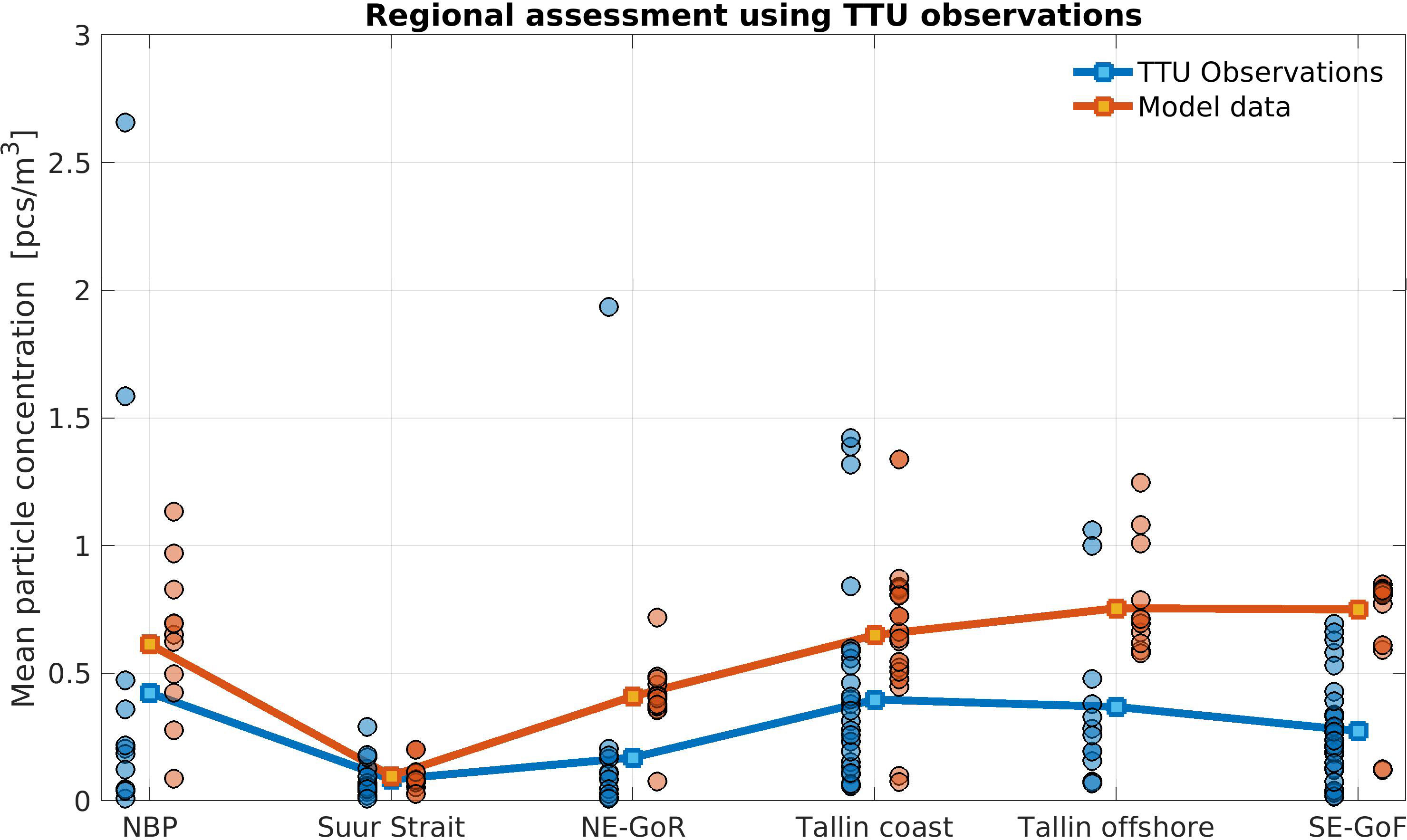
Figure 10 Comparison of modeled (red) and observed (blue) data sets from TalTech in Estonia. Regional averages are shown as solid lines, whereas individual observations and model data points are presented as red and blue dots.

The simulated spatial distribution (Figure 9B) also shows high concentrations in the NBP and southwestern GoF, and low concentrations in the Suur Strait and northern GoR. However, the model data have the highest concentration in southeastern GoF, mainly affected by the Neva and Narva. The model data show a similar pattern when compared with ferrybox data and LIAE data. The comparison of spatial distribution in TalTech data can be further illustrated by using subregional mean concentration (Figure 10). The analysis for the subregions shows that the NBP is the area with the highest mean observed concentration of 0.42 pcs/m³, whereas the lowest observed concentrations are found in Suur Strait 0.08 pcs/m³. In the NE-GoR, including a station near Pärnu, the concentrations increase to 0.17 pcs/m³. Further to the North, in the GoF, the observed concentrations increase toward Tallin coast 0.39 pcs/m³ and offshore 0.37 pcs/m³ and decrease toward Narva (SE-GoF) 0.27 pcs/m³. The model is able to reproduce the general features of the observed spatial pattern except for observed lows in the Narva area. The correlation between the averaged model and observation data sets for subregions is 0.81, with a P-value of 0.051. In the GoF, the west-eastern trend is reversed, showing an increase of modeled concentrations from 0.64 pcs/m³ at Tallin coast to 0.75 pcs/m³ at Tallin offshore and Narva (SE-GoF). To analyze this further, the model bias and the cRMSE, the root-mean-square error (RMSE) of the debiased data sets, are analyzed in more detail (Figs. 9C and 9D). cRMSE represents the errors originating from sample spread of model-observation differences, and is therefore affected by individual sampling and model errors, especially when the sample size is small. Model error statistics, in particular the model biases, are affected by the conversion from modeled mass concentrations to measured particle concentrations.

Near Tallin coast, in the southern Gulf of Finland (GoF), the cRMSE value is relatively large 0.37 pcs/m³, whereas the bias is 0.25 pcs/m³. Here, near the harbor, the variability across different samples is relatively high. The model cannot represent this. Further to the east, at Narva in the SE-GoF, the cRMSE is relatively low 0.24 pcs/m³, whereas the bias is larger 0.47 pcs/m³, indicating larger systematic differences between modeled and observed values. This might be due to an overestimation of the microplastic sources released by the Narva (river). The model biases in the Gulf of Finland near Narva (SE-GoF) are the highest in the entire study area. The second highest bias of 0.38 pcs/m³ occurs west of Narva, at Tallinn offshore station. Offshore transport with westerly currents from Narva station in the SE-GoF might affect the bias at the Tallin offshore station. The cRMSE 0.39 pcs/m³ is of the same size as the model bias, which indicates that the variability across samples is relatively large. The overestimation of riverine inputs of microplastic at Narva and the westwards transport of microplastics might be the reason why the model simulations show an increase of microplastic concentrations towards the east, from Tallin coast to Tallin offshore and SE-GoF (Figure 10), whereas the observed values are decreasing, along the southern side of the Gulf of Finland.

Seasonal variability

The seasonal pattern analysis provides an overview over the model’s ability to reproduce the seasonal dynamic in the Baltic Sea, controlled by river runoff and microplastic discharge as well as the seasonality of microplastic removal processes: biofouling, sinking, and sedimentation. For Estonian waters, an intercomparison of the monthly mean microplastic concentration of modeled and measured fragments is performed. Observations show a decrease of the microplastic fragment concentration from April to August and then an increase to September and October (Figure 11). The model data show a similar feature from April to September. However, the modeled concentration in October is lower than the one that is observed.

FIGURE 11

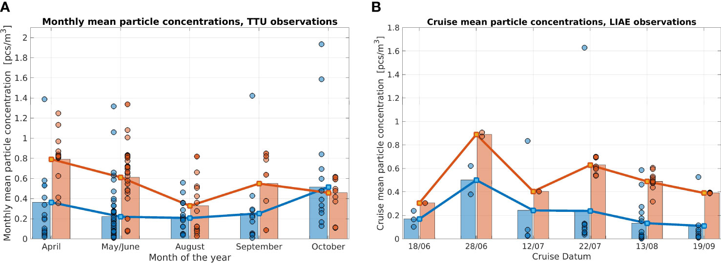
Figure 11 Comparison of observed (blue) and modeled (red) data sets from TalTech in Estonia (A) and from LIAE in Latvia (B). Monthly averages (left) and cruise averages (right) are shown as solid lines and bars, whereas individual observations and model data points are presented as red and blue dots.

For Latvia waters, an intercomparison was performed for the cruise mean microplastic fragment concentration, representing an averaged condition in the cruise-observed areas. Since the six cruises represent sampling from mid-June to late September in 2016, the comparison shows the model’s capacity on reproducing the microplastic variability in summer. The results show a similar pattern of temporal variation in summer 2018 between the model and observations: an increase of microplastic concentration from mid- to end of June, followed by a decrease to mid-July, an intermediate increase of modeled concentrations in the second half of July (cruise 4 in Figure 9) and a continuous decrease from August to September (Figure 11A). Cruise 4 in the second half of July extends offshore into the NBP. The P-value of the Pearson correlation test is 0.0145, which means that the correlation between the model and observed cruise means that the microplastic fragment concentration is significant at p< 0.05. It also means that the model is able to reconstruct a large part of the temporal variability of the mean microplastic condition in summer 2018 in the monitored areas.

Conclusions and discussions

In this work, a Eulerian model for the simulation of 3D transport and fate of microplastics in the marine environment has been introduced and assessed for the Baltic Sea. The model describes the wave- and current-induced transport of microplastics as well as the removal of microplastics through biofouling, sinking, and sedimentation processes. A multiyear model simulation in 2014–2019 was carried out, covering the entire Baltic Sea with an eddy-permitting resolution of 926 m to assess the spatial and seasonal pattern of microplastic pollution and to compare the model results with observations. Three categories of microplastic particles were considered: (1) small-sized particles with a diameter of 5 µm and density heavier than sea water, representing tire wear microplastics, (2) medium-sized particles with a diameter of 42 µm and density lighter than sea water, representing a majority of microplastic particles released from WWTPs, and (3) large-sized particles with a diameter of 300 µm and a density lighter than sea water, representing the large particle fraction released from WWTPs.

The model’s ability to reproduce the spatial pattern and the seasonal variability of observed microplastic pollution has been assessed for the large particle fraction. Since the model output is not exactly the same as the microplastic observations, a strict model validation is not possible in this paper. Only a model-observation intercomparison has been performed. It should be kept in mind that there are significant uncertainties in the individual observations, including 40%–56% sampling error, 12% surface flow correction error, and analysis error as shown in She et al. (2022). Statistically significant correlation was calculated for the modeled and observed TalTech data sets in 2016–2020. The results show that the model tends to be less good at simulating very high concentrations of microplastics than at simulating normal concentrations. The high microplastic concentration may be caused by flooding events near the shore or by submesoscale activities offshore, which require a higher model resolution and synoptic source information to be resolved.

Spatial patterns of modeled and observed distributions were analyzed for subregions, by grouping the data sets spatially to obtain more samples and to reduce the uncertainty of the intercomparison. The model is well able to reproduce the observed spatial pattern in the TalTech data set in the northern Baltic Proper, northern GoR, Suur Strait, and southwest GoF coastal waters. The coastal-offshore differences in the southwestern GoF, as observed by the ferrybox data, can also be simulated by the model. This suggests that model has a close-to-reality hydrodynamics, biofouling, and sedimentation in this part of the region. However, the discrepancy in the southeastern GoF coastal and offshore waters between the model and TalTech data suggests that improved circulation pattern in the eastern GoF and a better representation of the sources at Narva and the impacts of the Neva may be considered in more detail in the future studies.

The model is able to reconstruct the seasonal variability in summer months in both Latvian and Estonian waters. This suggests that the applied biofouling parameterization partially reflects the actual situation. The high microplastic concentration in October in Estonian waters is missed in the model data. One reason could be that the implemented biofilm growth model does not include processes such as grazing that remove biofilm from the particle surface. It is also noted that October is a month with peak activity on sub-mesoscale in this region (Karimova and Gade, 2015). The model setup in this study is too coarse to resolve submesoscales, which may be one of the reasons for the lower model skill in October.

Long-term simulations with constant microplastic concentrations in rivers have shown that the model converges to a seasonal quasi-equilibrium state in a weak sense, with removal processes balancing the coastal inputs into the Baltic Sea after an approximately 3.5-year spin-up, although a slight long-term trend still exists. The model has been tuned to reproduce the seasonal variability of microplastic in the Baltic Sea, the result of current- and wave-induced transport processes, mixing, and the seasonal dynamic of biofilm growth. A series of 3.5-year spin-up runs was performed to tune the removal processes of biofouling, sinking, and sedimentation. The tuning aimed at a stable seasonal cycle and a small (if not zero) long-term trend. There exist different results from monitoring data on the interannual variability of microplastic concentrations. Beer et al. (2018) found that the vertically integrated microplastic concentration have been “stationary” in the past 25 years in the Bornholm Basin, while a recent study showed that microplastic concentration in Estonian waters has decreased from year 2016 to year 2020 (Mishra et al., 2022). Further research, both from observation and modeling sides, is needed in order to identify the interannual variability of the microplastics in the sea.

Systematic microplastic transport assessments have been carried out to study the fate of microplastics at sea using the multiyear simulations. High concentrations were found near the surface in the vicinity of major coastal sources: large rivers, towns, and coastal outlets, particularly near WWTP, especially in metropolitan areas and other heavily populated regions. The entire Baltic Sea receives land-based microplastics from rivers and coastal catchments. In the southern and central Baltic Sea, the cyclonic circulation pattern spreads the plastic pollutants from main rivers: e.g., Oder and Vistula, and transports them along the shores of Poland, Lithuania, Latvia, and Estonia, eastwards and northwards to the sub-basins of the GoR, the GoF, and the Bay of Bothnia. Other heavy pollution patterns are found near major towns: e.g., Saint Petersburg, Helsinki, and Stockholm.

Offshore transport and sinking lead to the accumulation of microplastics in the deeper basins, mainly Bornholm Deep and Gothland Deep. Microplastics from major rivers in the southern Baltic Sea, Oder and Vistula, are gathered in the Bornholm Basin and are carried further into the Gothland Deep and further on into the GoF and the Bay of Bothnia. Household microplastics spread horizontally and settle onto the sediments in the biofilm growth season. First, it reaches the shallows, but, over time, it also fills the deeper basins. The annual cycle of river runoff and biofilm growth controls the modeled seasonality of seaborne microplastic pollution.

There are relatively large approximations in the implementations of modeling processes, and the specification of the land-based sources is simplified for the modeling study. The estimates for the amount of misused microplastics vary largely across different assessments. The cleaning capacities of WWTP needs to be taken into consideration to derive results adequate for detailed assessments. Another factor is the modeled size spectrum of microplastics, which reflects the average values obtained from bulk measurements in the effluents of WWTP and cannot represent the variability of microplastics in the marine environment. A broader spectrum of household microplastics with larger average sizes would better represent the observed particle concentrations in the ocean.

Uncertainties related to microplastic modeling are largely related to the implementation of biofouling, sedimentation/resuspension, and fragmentation processes. Household microplastics are introduced to the sea without a biofilm shell, which leads to somewhat-enhanced spreading while in their floating stage. High-resolution modeling on the estuary scale has shown that the modeling of biofouling and retention in rivers and estuaries can improve this (Frishfelds et al., 2022). Implementing an advanced biofilm growth model like in Kooi et al. (2014) should further advance this. The resuspension of microplastics in the sediment and fragmentation of macroplastics provide additional sources that have not been considered yet. Despite its shortcomings, the microplastic transport model and source mapping data set have been proven to provide a realistic drift pattern that can be used for the study of pathways of microplastic pollution.

Data availability statement

The raw data supporting the conclusions of this article will be made available by the authors, without undue reservation.

Author contributions

JM and JS designed the concept of the research. The HBM microplastic module and setup development and modeling experiment have been carried out by JM and VF. JS and JM specified microplastic sources and performed the validations. JS managed funding and administration. All authors contributed to the article and approved the submitted version.

Funding

The authors are grateful to be supported by the Horizon 2020 project “Cleaning Litter by developing and Applying Innovative Methods in European seas (CLAIM)” under Grant Agreement ID 774586. VF is grateful to be supported by the Latvian Fundamental and Applied Research Project lzp-2018/1-0162.

Conflict of interest

The authors declare that the research was conducted in the absence of any commercial or financial relationships that could be construed as a potential conflict of interest.

Publisher’s note

All claims expressed in this article are solely those of the authors and do not necessarily represent those of their affiliated organizations, or those of the publisher, the editors and the reviewers. Any product that may be evaluated in this article, or claim that may be made by its manufacturer, is not guaranteed or endorsed by the publisher.

References

Aigars J., Barone M., Suhareva N., Putna-Nimane I., Deimantovica-Dimante I. (2021). Occurrence and spatial distribution of microplastics in the surface waters of the baltic sea and the gulf of riga. Mar. pollut. Bull. 172, 112860. doi: 10.1016/j.marpolbul.2021.112860

PubMed Abstract | CrossRef Full Text | Google Scholar

Arheimer B., Pimentel R., Isberg K., Crochemore L., Andersson J. C. M., Hasan A., et al. (2019). Global catchment modelling using world-wide HYPE (WWH), open data and stepwise parameter estimation. Hydrol. Earth Syst. Sci. 24, 535–559. doi: 10.5194/hess-24-535-2020

CrossRef Full Text | Google Scholar

Axell L. B. (2002). Wind driven internal waves and langmuir circulations in a numerical ocean model of the southern Baltic Sea. J. Geophys. Res. 107 (C11), 3204. doi: 10.1029/2001JC000922

CrossRef Full Text | Google Scholar

BalMFC (2019) BALTICSEA_REANALYSIS_BIO_003_012: CMEMS Baltic Sea biogeochemistry reanalysis product, product user manual (PUM). Available at: http://marine.copernicus.eu/documents/PUM/CMEMS-BAL-PUM-003-012.pdf.

Google Scholar

BalMFC group, Leth O. K., Brüning T., Golbeck I., Jandt S., Janssen F., et al. (2014). My Ocean Baltic Sea Monitoring and Forecasting Centre, Conference: Operational Oceanography for Sustainable Blue Growth: The Seventh EuroGOOS Conference, 28-30 October 2014, At: Lisbon, Portugal, Volume: Proceedings of the seventh EuroGOOS Conference, Buch E, Antoniou Y, Eparkhina D, Nolan G (Eds.) ISBN 978-2-9601883-1-8, p33-42.

Google Scholar

Barnes D. K. A., Galgani F., Thompson R. C., Barlaz M. (2009). Accumulation and fragmentation of plastic debris in global environments. Philos. Trans. R. Soc B Biol. Sci. 364, 1985–1998. doi: 10.1098/rstb.2008.0205

CrossRef Full Text | Google Scholar

Beer S., Garm A., Huwer B., Dierking J., Nielsen T. G. (2018). No increase in marine microplastic concentration over the last three decades - a case study from the Baltic Sea. Sci. Total Environ. 621, 1272–1279. doi: 10.1016/j.scitotenv.2017.10.101

PubMed Abstract | CrossRef Full Text | Google Scholar

Berg P. (2012) Mixing in HBM. DMI scientific report no. 12-03. Available at: www.dmi.dk/file8admin/Rapporter/SR/sr12-03.pdf.

Google Scholar

Berg P., Poulsen J. W. (2012) Implementation details for HBM. DMI technical report no. Available at: www.dmi.dk/fileadmin/Rapporter/TR/tr12-11.pdf.

Google Scholar

Borrelle S. B., Ringma J., Law K. L., Monnahan C. C., Lebreton L., McGivern A., et al. (2020). Predicted growth in plastic waste exceeds efforts to mitigate plastic pollution. Science 369, 1515–1518. doi: 10.1126/science.aba3656

PubMed Abstract | CrossRef Full Text | Google Scholar

Brandon J. A., Jones W., Ohman M. D. (2019). Multidecadal increase in plastic particles in coastal ocean sediments. Sci. Adv. 5, eaax0587. doi: 10.1126/sciadv.aax0587

PubMed Abstract | CrossRef Full Text | Google Scholar

Brüning T. (2020). Improvements in turbulence model realizability for enhanced stability of ocean forecast and its importance for downstream components. Ocean Dynamics 70, 693–700. doi: 10.1007/s10236-020-01353-9

CrossRef Full Text | Google Scholar

Canuto V. M., Howard A., Cheng Y., Dubovikov S. (2001). Ocean turbulence. Part I: One-point closure model-momentum and heat vertical diffusivities. J. Phys. Oceanogr. 31, 240–264. doi: 10.1175/1520-0485(2001)031<1413:OTPIOP>2.0.CO;2

CrossRef Full Text | Google Scholar

Canuto V. M., Howard A., Cheng Y., Dubovikov S. (2002). Ocean turbulence. Part II: Vertical diffusivities of momentum, heat, salt, mass, and passive scalars. J. Phys. Oceanogr. 32, 240–264. doi: 10.1175/1520-0485(2002)032<0240:OTPIVD>2.0.CO;2

CrossRef Full Text | Google Scholar

Canuto V. M., Howard A. M., Cheng Y., Muller C. J., Leboissetier A., Jayne S. R. (2010). Ocean turbulence. III: New GISS vertical mixing scheme. Ocean Model. 34, 70–91. doi: 10.1016/j.ocemod.2010.04.006

CrossRef Full Text | Google Scholar

Craig P. D., Banner M. L. (1994). Modeling wave-enhanced turbulence in the ocean surface layer. J. Phys. Oceanogr. 24, 2546. doi: 10.1175/1520-0485(1994)024<2546:MWETIT>2.0.CO;2

CrossRef Full Text | Google Scholar

Craig D., Matthew M., John S., Jonah R.-J., Emma F., Werenfrid W., et al (2011). The Operational Sea Surface Temperature and Sea Ice Analysis (OSTIA) system. Remote Sensing of Environment 116, 114–158. doi: 10.1016/j.rse.2010.10.017

CrossRef Full Text | Google Scholar

Cubarenko I., Bagaev A., Zobkov M., Esiukova E. (2016). On some physical and dynamical properties of microplastic particles in marine environment. Mar. pollut. Bull. 108, 105–112. doi: 10.1016/j.marpolbul.2016.04.048

PubMed Abstract | CrossRef Full Text | Google Scholar

Cuttat F. M. R. (2018). Marine transport of plastic fragments from dolly ropes used in demersal fisheries in the north Sea (Denmark: DTU Aqua). Available at: http://infoscience.epfl.ch/record/264490

Google Scholar

Dang H., Lovell C. R. (2015). Microbial surface colonization and biofilm development in marine environments. ASM J. Microbiol. Mol. Biol. Rev. 80, 91–138. doi: 10.1128/MMBR.00037-15

CrossRef Full Text | Google Scholar

Danish Environmental Protection Agency (EPA) (2015). Microplastics occurrence, effects and sources of releases to the environment in Denmark environmental project no. 1793 (Copenhagen, Denmark: The Danish Environmental Protection Agency)

Google Scholar

Derraik J. G. (2002). The pollution of the marine environment by plastic debris: a review. Mar. pollut. Bull. (The Danish Environmental Protection Agency, Strandgade: Copenhagen K) 44, 842–852. doi: 10.1016/S0025-326X(02)00220-5. www.eng.mst.dk

PubMed Abstract | CrossRef Full Text | Google Scholar

EU Commission (2008). Directive 2008/56/EC of the European parliament and of the council. Of J. Eur. Union 164, 19–40. Available at: http://data.europa.eu/eli/dir/2008/56/oj

Google Scholar

Fischer M., Friedrichs G., Lachnit T. (2014). Fluorescence-based quasicontinuous and In situ monitoring of biofilm formation dynamics in natural marine environments. Appl. Environ. Microbiol 80 (12), 3721–3728. doi: 10.1128/AEM.00298-14

PubMed Abstract | CrossRef Full Text | Google Scholar

Frishfelds V., Murawski J., She J. (2022). Transport of microplastics from the daugava estuary to the Open Sea. American Society for Microbiology Applied and Environmental Microbiology 80 (12), 3721–3728. doi: 10.3389/fmars.2022.886775

CrossRef Full Text | Google Scholar

Gayer G., Dick S., A. Pleskachevsky A., Rosenthal W. (2006). Numerical modeling of suspended matter transport in the north sea. Ocean Dynamics 56, 62–77. doi: 10.1007/s10236-006-0070-5

CrossRef Full Text | Google Scholar

Geyer R., Jambeck J. R., Law K. L. (2017). Production, use, and fate of all plastics ever made. Sci. Adv. 3, e1700782. doi: 10.1126/sciadv.1700782

PubMed Abstract | CrossRef Full Text | Google Scholar

Halle A. T., Ladirat L., Gendre X., Goudouneche D., Pusineri C., Routaboul C., et al. (2016). Understanding the fragmentation pattern of marine plastic debris. Environ. Sci. Technol. 50, 5668–5675. doi: 10.1021/acs.est.6b00594

PubMed Abstract | CrossRef Full Text | Google Scholar

HELCOM (2009). Marine litter in the Baltic Sea region (Baltic Marine Environment Protection Commission (Helsinki, Finland:HELCOM ). 20 pp. Available at: https://portal.helcom.fi/meetings/PRESSURE%2010-2019-549/MeetingDocuments/6-6-Att.%20Background%20information%20of%20the%20Baltic%20Sea%20catchment%20area%20for%20the%20Sixth%20Baltic%20Sea%20Pollution%20load%20compilation%20(PLC-6).pdf

Google Scholar

HELCOM (2019). Background information on the Baltic Sea catchment area for the sixth Baltic Sea pollution load compilation (PLC-6) (Baltic Marine Environment Protection Commission (HELCOM). Available at: https://portal.helcom.fi/meetings/PRESSURE%2010-2019-549/MeetingDocuments/6-6-Att.%20Background%20information%20of%20the%20Baltic%20Sea%20catchment%20area%20for%20the%20Sixth%20Baltic%20Sea%20Pollution%20load%20compilation%20(PLC-6).pdf.

Google Scholar

Hinata H., Mori K., Ohno K., Miyao Y., Kataoka T. (2017). An estimation of the average residence times and onshore-offshore diffusivities of beached microplastics based on the population decay of tagged meso- and macrolitter Mar. pollut. Bull. 122, 17–26. doi: 10.1016/j.marpolbul.2017.05.012.

PubMed Abstract | CrossRef Full Text | Google Scholar

Jambeck J. R., Geyer R., Wilcox C., Siegler T. R., Perryman M., Andrady A., et al. (2015). Marine pollution. Plast. waste inputs land into ocean. Sci. 347, 768–771. doi: 10.1126/science.1260352

CrossRef Full Text | Google Scholar

Karimova S., Gade M. (2015). Analysis of sub-mesoscale eddies in the Baltic Sea based on SAR imagery and model wind data. International Journal of Remote Sensing 37, 2394–2414. doi: 10.1080/01431161.2016.1145367

CrossRef Full Text | Google Scholar

Karlsson T., Kärrman A., Rotander A., Hassellöv M. (2020). Comparison between manta trawl and in situ pump filtration methods, and guidance for visual identification of microplastics in surface waters. Environ. Sci. pollut. Res. 27, 5559–5571. doi: 10.1007/s11356-019-07274-5

CrossRef Full Text | Google Scholar

Kaza S., Yao L., Bhada-Tata P., Van Woerden F. (2018). What a waste 2.0: A global snapshot of solid waste management to 2050. overview booklet (Washington, DC: World Bank).

Google Scholar

Kole P. J., Löhr A. J., Van Belleghem F. G.A.J., Ragas A. M.J. (2017). Wear and tear of tyres: A stealthy source of microplastics in the environment. Int J Environ Res Public Health. 14 (10), 1265. doi: 10.3390/ijerph14101265

CrossRef Full Text | Google Scholar

Komen G. J., Cavaleri L., Donelan M., Hasselmann K., Hasselmann S., Janssen P. A. E. M. (1994). Dynamic and modelling of ocean waves, book (Cambridge University Press). doi: 10.1017/CBO9780511628955

CrossRef Full Text | Google Scholar

Kooi M., van Nes E. H., Scheffer M., Koelmans A. A. (2014). Ups and downs in the ocean: Effects of biofouling on vertical transport of microplastics. Environ. Sci. Technol. 51, 7963–7971. doi: 10.1021/acs.est.6b04702

CrossRef Full Text | Google Scholar

Lebreton L. C.M., Zwet J.-W. D., Slat B., Andrady A., Reisser J.. (2017). River plastic emissions to the world’s oceans. Nat. Commun. 8, 15611. doi: 10.1038/ncomms15611

PubMed Abstract | CrossRef Full Text | Google Scholar

Magnusson K., Wahlberg C. (2014). Mikroskopiska skräppartiklar i vatten från avloppsreningsverk (Microscopic litter particles in water from WWTPs) in Swedish, IVL Swedish environmental research institute. Rep. B 2208, 30.

Google Scholar

Mishra A., Buhhalko N., Lind K., Lips I., Liblik T., Väli G., et al. (2022). Spatiotemporal variability of microplastics in the Eastern Baltic Sea. Front. Mar. Sci. 9. doi: 10.3389/fmars.2022.875984

PubMed Abstract | CrossRef Full Text | Google Scholar

Nerland I. L., Halsband C., Allan I., Thomas K. V. (2014). Microplastics in Marine Environments: Occurrence, Distribution and Effects. (Oslo, Norway: Norwegain Institute of Water Research) 73 p. Available at: https://www.miljodirektoratet.no/globalassets/publikasjoner/M319/M319.pdf

Google Scholar

OC-TAC(2019). OCEANCOLOUR_BAL_OPTICS_L3_REP_OBSERVATIONS_009_097, CMEMS satellite-based chlorophyll-a product for the Baltic Sea, product user manual (PUM). Available at: http://marine.copernicus.eu/documents/PUM/CMEMSOC-.PUM-009-ALL.pdf

Google Scholar

Osinski R. D., Enders K., Gräwe U., Klingbeil K., Radtke H. (2020). Model uncertainties of a storm and their influence on microplastics and sediment transport in the baltic sea. Ocean Sci. 16, 1491–1507. doi: 10.5194/os-16-1491-2020

CrossRef Full Text | Google Scholar

OSPAR, Verschoor A., van Herwijnen R., Posthuma C., Klesse K., Werner S. (2017). Assessment document of land-based inputs of microplastics in the marine environment, environmental impact of human activities series (OSPAR Convention).

Google Scholar

Parker-Jurd F., Napper I., Abbott G., Hann S., Thompson R. (2021). Quantifying the release of tyre wear particles to the marine environment via multiple pathways. Mar. pollut. bull. 172, 112897. doi: 10.1016/j.marpolbul.2021.112897

PubMed Abstract | CrossRef Full Text | Google Scholar

Pleskachevsky A., Gayer G., Horstmann J., Rosenthal W. (2005). Synergy of satellite remote sensing and numerical modelling for monitoring of suspended particulate matter. Ocean Dynamics 55, 2–94. doi: 10.1007/s10236-004-0101-z

CrossRef Full Text | Google Scholar

Poulsen J. W., Berg P. (2012) More details HBM – general modelling theory and survey of recent studies. technical report. Available at: http://beta.dmi.dk/fileadmin/Rapporter/TR/tr12-16.pdf.

Google Scholar

Poulsen J. W., Berg P., Raman K. (2015). Better concurrency and SIMD on HBM”, chapter 3 in “High performance parallelism pearls - multicore and many-core programming approaches Elsevier. Eds. Jeffers J., Reinders J. (Morgan Kaufmann). Available at: https://books.google.se/books/about/High_Performance_Parallelism_Pearls_Volu.html?id=R-99BAAAQBAJ&printsec=frontcover&source=kp_read_button&hl=en&redir_esc=y#v=onepage&q&f=false

Google Scholar

Schaffer J., Timmermann R. (2016). Greenland And Antarctic ice sheet topography, cavity geometry, and global bathymetry (RTopo-2), links to NetCDF files (PANGAEA). doi: 10.1594/PANGAEA.856844

CrossRef Full Text | Google Scholar

Schaffer J., Timmermann R., Arndt J. E., Kristensen S. S., Mayer C., Morlighem M., et al. (2016). A global, high-resolution data set of ice sheet topography, cavity geometry, and ocean bathymetry. Earth Syst. Sci. Data 8 (2), 543–557. doi: 10.5194/essd-8-543-2016

CrossRef Full Text | Google Scholar

Schernewski G., Radtke H., Hauk R., Baresel C., Olshammar M., Oberbeckmann S. (2021). Urban microplastics emissions: Effectiveness of retention measures and consequences for the Baltic Sea. Front. Mar. Sci. 8. doi: 10.3389/fmars.2021.594415

PubMed Abstract | CrossRef Full Text | Google Scholar

Setälä O., Magnusson K., Lehtiniemi M., Norén F. (2016). Distribution and abundance of surface water microlitter in the Baltic Sea: a comparison of two sampling methods. Mar. pollut. Bull. 110, 177–183. doi: 10.1016/j.marpolbul.2016.06.065

PubMed Abstract | CrossRef Full Text | Google Scholar

She J., Buhhalko N., Lind K., Mishra A., Kikas A., Costa E., et al. (2022). Uncertainty and consistency assessment in multiple microplastic observation datasets in the Baltic Sea. Frontier Mar. Sci 9, 886357. doi: 10.3389/fmars.2022.886357

CrossRef Full Text | Google Scholar

She J., Murawski J. (2018). “Towards seamless modelling for the Baltic Sea” Proceedings of the Eight EuroGOOS International Conference in Operational Oceanography serving Sustainable Marine Development, Bergen, Norway (Brussels, Belguim: EuroGOOS AISBL) 3-5, 233–241.

Google Scholar

She J., Murawski J., Lips I. (2021). Marine plastic litter source dataset in the Baltic and Mediterranean Sea, part b: Baltic sea. CLAIM report D1.2. p154.

Google Scholar

Siegfried M., Koelmans A. A., Besseling E., Kroeze C. (2017). Export of microplastics from land to sea. a modelling approach. Water Res. 127, 249–257. doi: 10.1016/j.watres.2017.10.011

PubMed Abstract | CrossRef Full Text | Google Scholar

Smagorinsky J. (1963). General circulation experiments with the primitive equations. Monthly Weather Rev. 91 (3), 99–164. doi: 10.1175/1520-0493(1963)091<0099:GCEWTP>2.3.CO;2

CrossRef Full Text | Google Scholar

Talvitie J., Heinonen M., Paakkonen J. P., Vahtera E., Mikola A., Setala O., et al. (2015). Do wastewater treatment plants act as a potential point source of microplastics? preliminary study inthe coastal gulf of Finland, Baltic Sea. Water Sci. Technol. 72 (9), 1495–1504. doi: 10.2166/wst.2015.360

PubMed Abstract | CrossRef Full Text | Google Scholar

Tsiaras K., Hatzonikolakis Y., Kalaroni S., Pollani A., Triantafyllou G. (2021). Modeling the pathways and accumulation patterns of micro- and macro-plastics in the mediterranean. Front. Mar. Sci. 8, 152. doi: 10.3389/fmars.2021.743117

CrossRef Full Text | Google Scholar

Vollertsen J., Hansen A. A. (2017).“Microplastic in Danish wastewater; sources, occurences and fate”, in Environmental project no. 1906 (The Danish Environmental Protection Agency).

Google Scholar

WAMDI Group (1988). The WAM model – a third generation ocean wave prediction model. JPO 18 (12), 1775–1810. doi: 10.1175/1520-0485(1988)018<1775:TWMTGO>2.0.CO;2

CrossRef Full Text | Google Scholar