Coupled Carbonate Chemistry - Harmful Algae Bloom Models for Studying Effects of Ocean Acidification on Prorocentrum minimum Blooms in a Eutrophic Estuary

Introduction

The frequency, duration, and intensity of harmful algal blooms (HABs) have increased due to eutrophication as well as global climate change in recent decades (Glibert and Burford, 2017; Glibert, 2020). Climate change is impacting HABs in complex ways, from warming of waters, to changing precipitation patterns and changing stratification (Paerl and Huisman, 2008; Wells et al., 2015; Glibert, 2020). Ocean acidification (OA), a consequence of oceanic uptake of excess atmospheric CO₂, could also contribute to the global expansion of HABs, but its effects on HABs are not as well understood as other climate change factors.

CO₂ enrichment is expected to relieve the energy requirements of photosynthesis, especially of those primary producers that rely on carbon concentrating mechanisms (CCMs) to overcome inorganic C limitation. CCMs increase the concentration of CO₂ at the site of Rubisco, the primary carboxylating enzyme in photosynthesis. In particular, those species having Form II Rubisco, which has a lower affinity for CO₂ than form I, would be expected to benefit when CO₂ is enriched (Tortell, 2000; Rost et al., 2003; Giordano et al., 2005; Raven and Beardall, 2014). Many bloom-forming dinoflagellates fall into this category and rising CO₂ could stimulate the growth of these species. In addition to impacting C fixation, decreasing pH also could influence algal growth by affecting nutrient uptake. Lowered pH could affect nutrient acquisition by altering the cellular transmembrane potential, enzyme activity (Beardall and Raven, 2004; Giordano et al., 2005), or chemical speciation of dissolved nutrients (Shi et al., 2010). Despite the varied effects of increasing CO₂ on dinoflagellates and their complex physiological responses, limited previous studies suggested that OA could stimulate the growth of many HAB species (e.g. Beardall et al., 2009; O'Neil et al., 2012; Wells et al., 2015; Glibert, 2020).

During the past half-century, levels of atmospheric and surface water CO₂ concentrations have increased by more than 25%, lowering pH in the ocean by about 0.1 unit (Doney et al., 2012; Takahashi et al., 2014; Bates et al., 2014; Doney et al., 2020). Surface water pH of the ocean is expected to decrease further by 0.3 – 0.4 unit by the end of the 21^st century (Feely et al., 2004; Feely et al., 2009; Jiang et al., 2019; IPCC, 2021). Compared with the open ocean, coastal and large estuaries are experiencing an accelerated pace of acidification, as organic matter respiration contributes to dissolved inorganic C production, in addition to CO₂ uptake from the atmosphere (Cai et al., 2011; Cai et al., 2017; Cai et al., 2021). Therefore, eutrophication exerts a dual effect on estuaries and coastal oceans, not only stimulating HABs but also exacerbating OA. Chesapeake bay, the largest estuary in the U.S., which suffers from both OA and HABs, provides an excellent system to investigate the impacts of OA on HAB abundance and distribution.

Recent observations in Chesapeake bay found pH and surface pCO₂ to have large spatial gradients and strong temporal variabilities (Brodeur et al., 2019; Huang et al., 2019; Shadwick et al., 2019; Chen et al., 2020; Friedman et al., 2020). The pH range is large, with a minimum value of 7.1 in the upper bay and the bottom waters of the mid bay and a maximum value as high as 8.5 in the surface waters of the mid and lower bay (Brodeur et al., 2019). pCO₂ also displays a strong along-channel gradient from the estuary’s head to mouth, resulting in outgassing in the upper bay, uptake of atmospheric CO₂ in the mid bay, and near-equilibrium conditions in the lower bay (Cai et al., 2017; Chen et al., 2020; Friedman et al., 2020). Observations from a moored sensor showed high frequency fluctuations of pH and pCO₂, driven by a wide array of physical and biological processes (Shadwick et al., 2019).

Modeling studies and retrospective data analysis have shown significant but complex long-term pH trends in Chesapeake bay over the past three decades (Shen et al., 2020; Da et al., 2021). In the upper bay, where pH in near-surface waters has historically been low, there has been a long-term increase (basification), influenced by freshwater input and increasing alkalinity in the Susquehanna River (Kaushal et al., 2013). In contrast, in the lower bay, which historically had a higher pH, there has been a decrease in pH and acidification due to oceanic influence. Due to the counter-balance between OA and river alkalinization (Shen et al., 2020), pH in the autotrophic mid-bay has shown no significant long term trends but displays strong short-term fluctuations likely associated with phytoplankton photosynthesis. Also, seasonally, calcium carbonate dissolution is an important buffering mechanism for pH changes in late summer in the mid-bay, leading to higher pH values in August than in June, despite persistent hypoxic conditions during the summer (Su et al., 2020; Su et al., 2021). How these long term pH trends and seasonal variations affect seasonal development of HABs and how the increasing atmospheric pCO₂ in a warming climate influence HABs are largely unknown but are of critical importance for managing coastal resources.

Prorocentrum minimum, a species of increasing global concern (Heil et al., 2005; Glibert et al., 2008; Glibert et al., 2012), is one of the major bloom-forming harmful dinoflagellates of Chesapeake bay. Blooms of P. minimum can lead to hypoxic events, death of finfish and shellfish, and submerged aquatic vegetation losses (Tango et al., 2005). Such blooms are restricted to certain ranges of temperature and salinity, and occur most frequently in April and May (Tango et al., 2005; Li et al., 2015). Bloom events of this species have increased from ~13 per year in the 1990s to > 20 per year in the early 2000s in Chesapeake bay (Li et al., 2015). However, the effects of pH on P. minimum growth have been seldom investigated although there were some laboratory experimental studies. Under high pH, growth of P. minimum is greatly reduced, while its growth rate increases moderately as pH decreases (Hansen, 2002). Fu et al. (2008) found CO₂ enrichment could increase the growth rate of P. minimum by increasing its maximum light-saturated C fixation rate. Later experiments found extremely low pH (< 7) could also limit growth of dinoflagellates, but P. minimum was able to survive under such conditions (Berge et al., 2010). These laboratories studies were conducted with P. minimum under fixed values of pH or CO₂ concentration. It remains unclear how P. minimum is affected by varying pH level in situ in an estuarine environment as it is transported in the estuary and its position varies seasonally (Tyler and Seliger, 1978; Zhang et al., 2021; Li et al., 2021). A mechanistic model that integrates hydrodynamics, carbonate chemistry and harmful algae physiology is needed to address such questions.

Few plankton models have explicitly incorporated the effects of pH or pCO₂ and have been mainly used to interpret results obtained from controlled laboratory experiments (e.g. Schippers et al., 2004; Flynn et al., 2015; Almomani, 2019). In this study we developed a new integrated modeling system to investigate the effects of OA on P. minimum blooms in vivo, by coupling 3D hydrodynamic, carbonate chemistry and HAB models. The model results provide a first glimpse into the effects of OA on HABs in a dynamic and variable present and future estuarine environment. The modeling system is based on widely used ocean models and can be readily applied to other estuaries and coastal oceans.

Methods

The integrated modeling system consists of four submodels: a hydrodynamic model based on the Regional Ocean Modeling System (ROMS) (Shchepetkin and McWilliams, 2005; Haidvogel et al., 2008); a biogeochemical model based on the Row Column Aesop (RCA) structure (Di Toro, 2001; Isleib et al., 2007; Testa et al., 2014); a carbonate chemistry (CC) model based on Shen et al. (2019a); and a HAB model based on a mechanistic model developed by Zhang et al. (2021). This integrated modeling system is termed ROMS-RCA-CC-Prorocentrum (Figure 1).

FIGURE 1

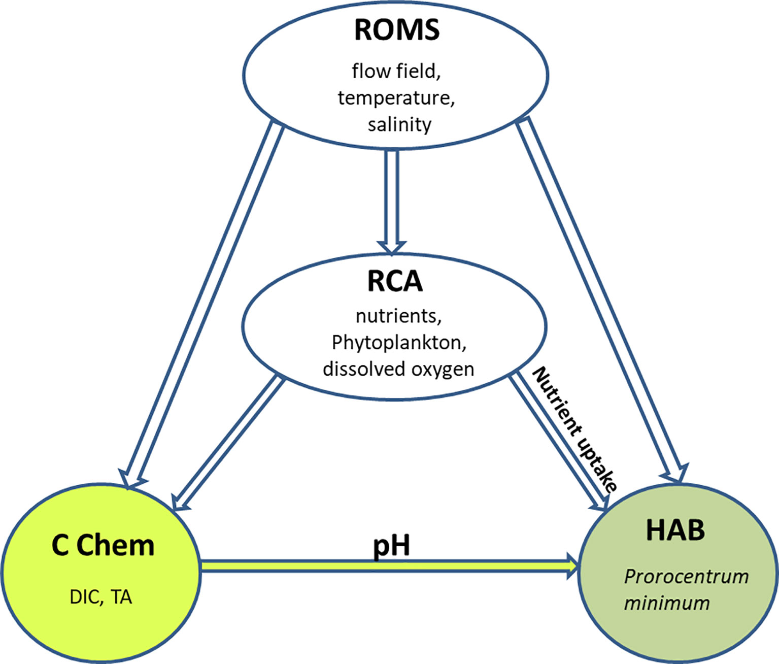
Figure 1 A conceptual diagram of the ROMS-RCA-CC-Prorocentrum coupled model: ROMS is the hydrodynamic model, RCA is the biogeochemical model, CC is the carbonate chemistry model, and HAB is the model for P. minimum.

Hydrodynamic Model (ROMS)

The ROMS hydrodynamic model was configured for Chesapeake bay and its adjacent shelf (Figure 2), consisting of 80 × 120 grid points in the horizontal direction and 20 evenly distributed vertical sigma levels in the vertical direction (Li et al., 2005). An orthogonal curvilinear coordinate system was used to follow the general orientation of the deep channel and the coastlines of the main stem of the bay. Coastal boundaries were specified as a finite-discretized grid via land/sea masking.

FIGURE 2

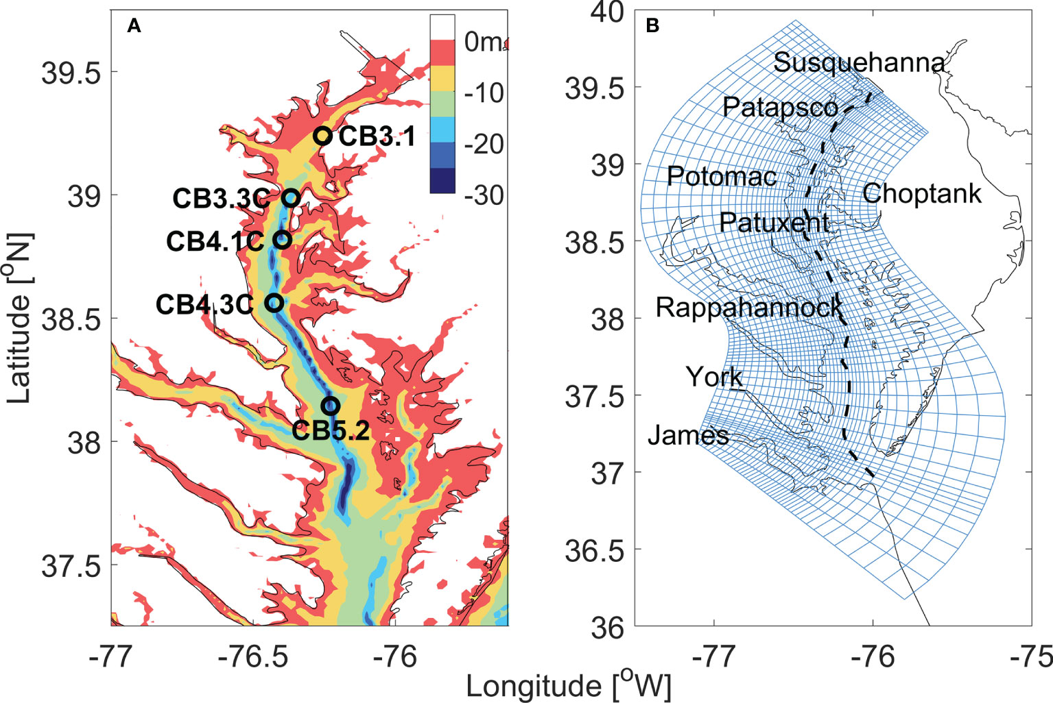
Figure 2 (A) The bathymetry of Chesapeake bay. The open circles mark the location of five sites along the main stem. (B) The horizontal curvilinear coordinate system for ROMS-RCA model, every third grid line is plotted in both along- and cross-bay directions. The black dashed line marks the location of the along-channel section used in later analysis.

ROMS is forced by freshwater discharge at river heads, water levels at the open boundary, and heat and momentum flux across the sea surface. The freshwater input was prescribed for the eight major tributaries of Chesapeake bay, based on measurements at US Geological Survey gaging stations (USGS). The offshore boundary water level consists of tidal and non-tidal components. The tidal component was provided by global tidal model TPXO7 (TOPEX/POSEIDON) (Egbert and Erofeeva, 2002), and the non-tidal component was extracted from daily sea level measured at Duck, North Carolina, by the National Oceanic and Atmospheric Administration (NOAA). The air-sea heat flux and momentum flux were computed by using the North America Regional Reanalysis (NARR) data. The vertical eddy viscosity and diffusivity were parameterized using the k-kl turbulence closure scheme with the background value of 1 × 10^-6 m² s^-1, and the horizontal eddy viscosity and diffusivity were set to be constant (1 m² s^-1). The ROMS model was initialized using climatological temperature and salinity conditions and run for a spin-up period of 2 years to get the initial condition for year 2006. A detailed description of the model configuration can be found in Li et al. (2005). This hydrodynamic model was previously validated against water level measurements at tidal gauge stations (Zhong and Li, 2006; Zhong et al., 2008), salinity and temperature time series at monitoring stations (Li et al., 2005; Ni et al., 2020), salinity distributions collected during hydrographic surveys, and current measurements (Li et al., 2005; Xie and Li, 2018; Xie and Li, 2019), including the year of 2006 (Ni et al., 2020).

Biogeochemical Model (RCA)

The RCA biogeochemical model includes a water-column component (Isleib et al., 2007) and a sediment diagenesis component (Di Toro, 2001), coupled to the ROMS hydrodynamic model in an offline mode. RCA simulates pools of organic and inorganic nutrients, two phytoplankton groups (one representing winter-spring diatoms and one representing summer dinoflagellates), and dissolved oxygen concentrations (Testa et al., 2014). The RCA biogeochemical model is forced by loads of dissolved and particulate materials from the eight major rivers. Riverine constituent concentrations for phytoplankton, silica, particulate and dissolved organic C, phosphorus (P), and nitrogen (N), and inorganic nutrients $\left[{\text{NH}}_4^{+},{\text{NO}}_2^{-}+{\text{NO}}_3^{-}\text{hereafter\hspace{0.17em}}{\text{NO}}_3^{-},{\text{PO}}_4^{3-}\right]$ were obtained or derived from Chesapeake bay Program biweekly monitoring data as described in Testa et al. (2014). The ocean boundary concentrations were acquired from the World Ocean Atlas 2013 and Filippino et al. (2011). Atmospheric deposition of nutrients was much smaller than the riverine nutrient loading and thus not considered, following the previous studies (Ni et al., 2020; Li et al., 2020b; Zhang et al., 2021). The initial conditions of RCA were based on Chesapeake bay Program monitoring data in December 2005. The RCA model has been validated against biogeochemical data at a number of stations in Chesapeake bay (including ${\text{NO}}_3^{-}$, ${\text{PO}}_4^{3-}$, ${\text{NH}}_4^{+}$, chlorophyll-a, dissolved oxygen, and organic C, N and P), integrated metrics of hypoxic volume, rates of water-column primary production and respiration, and nutrient fluxes across the sediment-water surface (Brady et al., 2013; Testa et al., 2013; Testa et al., 2014; Li et al., 2016; Testa et al., 2017; Ni et al., 2020).

Carbonate chemistry Model (CC)

The CC model simulates Dissolved Inorganic Carbon (DIC), Total Alkalinity (TA), and mineral calcium carbonate (aragonite CaCO₃) and has previously been coupled to ROMS-RCA for Chesapeake bay (Shen et al., 2019a; Shen et al., 2019b; Shen et al., 2020). DIC is consumed by phytoplankton growth/photosynthesis and calcium carbonate precipitation. The sources of DIC include air-sea CO₂ flux, phytoplankton respiration, oxidation of organic matter, calcium carbonate dissolution, sulfate reduction, and sediment water fluxes. Calcium carbonate dissolution and precipitation are the primary source/sinks for TA, but the contributions of several other biogeochemical processes (e.g., nitrification and sulfate reduction) to TA are also modeled. Other carbonate chemistry parameters such as pH and pCO₂ are calculated from the CC model outputs using the CO2SYS program (Lewis and Wallace, 1998). A detailed description of the CC model and its coupling to RCA is described in Shen et al. (2019a). The CC model is forced by the atmospheric CO₂, the riverine loads and offshore concentration of TA and DIC. Time series of TA measurements in riverine inputs were obtained from the USGS stations in the Susquehanna and Potomac Rivers (Raymond et al., 2000). The riverine DIC concentrations were calculated through CO2SYS with the available TA and pH (Shen et al., 2020). Carbonate chemistry data for the other smaller tributaries were estimated using empirical relationships as functions of freshwater discharge (Shen et al., 2019a). TA at the ocean boundary was directly estimated with the empirical equation based upon salinity at the ocean boundary (Cai et al., 2010). DIC at the offshore boundary was calculated with the available TA, fCO₂ from SOCAT (Bakker et al., 2016), salinity and temperature using CO2SYS. The atmosphere pCO₂ was set to be 400 ppm in 2006, a year chosen for historical validation, according to the observation from NOAA-ESRL (https://www.esrl.noaa.gov/gmd/ccgg/trends; Li et al., 2020a). Initial conditions for DIC and TA were calculated from the two-end member mixing model. The CC model has been validated against extensive surveys of DIC, TA and pH collected during ten cruises in 2016 (Shen et al., 2019a) and long term (1985-2015) measurements of pH at a number of monitoring stations (Shen et al., 2019b; Shen et al., 2020).

P. minimum Model (HAB) Incorporating pH Effects

The P. minimum model is a mechanistic HAB model that has previously been embedded within RCA for Chesapeake bay (Zhang et al., 2021). A rhomboid strategy was used: that is, P. minimum is modeled individually while the two other plankton populations (winter diatoms and summer dinoflagellates) are represented by the aggregate functional classes. The model parameters for P. minimum are given in Zhang et al. (2021) and the parameters for the winter-spring diatoms and summer dinoflagellates can be found in Testa et al. (2014).

For the P. minimum model, the growth rate depends on temperature, light and nutrient concentrations, while the mortality terms include both grazing and respiration, and the model parameters have been calibrated according to published physiological experiments on P. minimum and numerical sensitivity-analysis experiments. The equation for P. minimum biomass is given by

$\begin{array}{ll}\frac{d\left(proro\right)}{dt}=G\ast proro-R_{res}\ast proro-R_{gz}\ast pror{o}^2& (1)\end{array}$

where proro is the biomass of P. minimum measured by carbon (in unit of mgC L^-1), G is the growth rate, R_res is the respiration rate, and R_gz is the grazing rate. To include the effects of pH on P. minimum growth, G is calculated as

$\begin{array}{ll}G=G_T\ast G_{par}\ast G_N\ast G_{pH}& (2)\end{array}$

where G_T is the specific growth rate depending on temperature, G_par represents the effects of light availability, G_N represents the effects of nutrient limitation on growth, and G_pH represents the effects of pH on growth. The formulae for G_T, G_par and G_N can be found in Zhang et al. (2021). In Eq. (2) G_T and G_pH were assumed to be independent of each other, but some previous laboratory experiments showed that elevated CO₂ alone led to a higher growth rate but elevated CO₂ in concert with temperature increase had no significant effect on P. minimum growth (Fu et al., 2008). Equation (2) can be readily modified to consider nonlinear interactions between higher CO₂ and warming when more experimental data are available.

G_pH was estimated by fitting an empirical relation to previously published experimental data on P. minimum culture grown under different pH conditions (Hansen, 2002; Berge et al., 2010; Figure 3). In those experiments, P. minimum growth rates were obtained in a laboratory setting under a range of pH conditions while other parameters such as temperature and salinity were held at fixed values. To capture the sole effect of pH on the growth rate, G_pH was normalized by the respective mean value in each laboratory experiment such that P. minimum growth is enhanced by OA when G_pH > 1 but suppressed by it when G_pH < 1. pH values in Hansen’s (2002) experiments ranged from 7 – 10, far beyond the pH range observed in Chesapeake bay, but only experimental data in the pH range of 7.2 – 8.5 are shown in Figure 3. G_pH increased by about 10% as pH decreased from 8.5 to 7.2, representing a modest enhancement of growth rate.

FIGURE 3

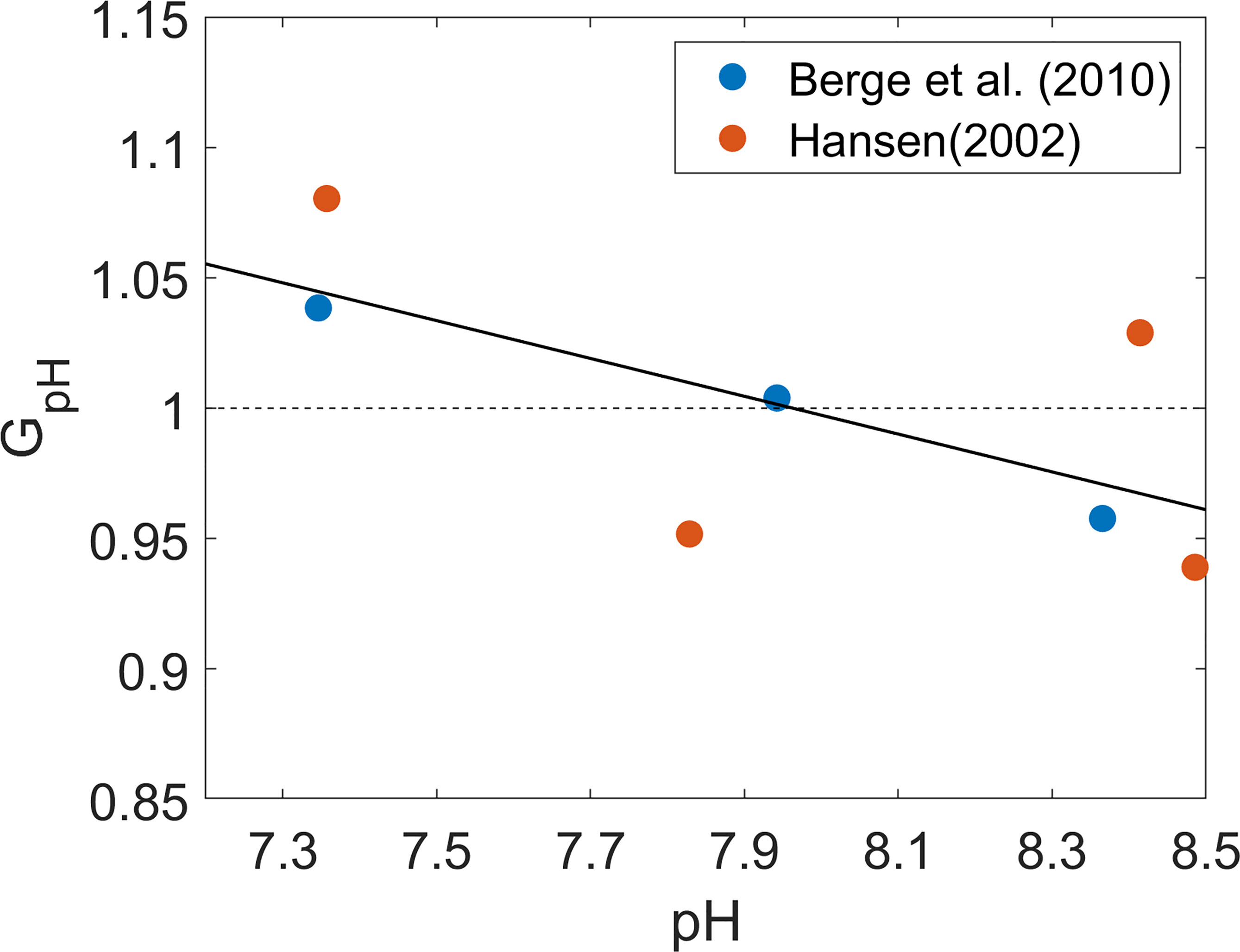
Figure 3 Normalized growth rate of P. minimum (G_pH) as a function of pH. Blue open circles represent data from Berge et al. (2010) and red open circles represent data from Hansen (2002). Both growth rates were normalized by the corresponding mean growth rate under pH ranging from 7 to 8.5 which is a typical range of Chesapeake bay water pH. Solid black line is the fitted curve which was used in the model considering pH effects.

The boundary conditions for P. minimum at the river heads and continental shelf were set to 0. The initial condition of P. minimum for the entire estuary were interpolated using the distribution reported in the estuary-wide surveys reported in Tyler and Seliger (1978). Model sensitivity-analysis experiments in Zhang et al. (2021) showed that the prediction of P. minimum blooms is insensitive to the initial condition as long as a small seed population exists at the beginning of the year.

Numerical Runs

The new coupled models were first used to conduct a hindcast simulation for the year 2006. The results were used to compare with the simulations by the original ROMS-RCA-Prorocentrum model which did not consider pH effects (Zhang et al., 2021).

To project the future effects of OA on P. minimum blooms, two climate projection runs were conducted by increasing the atmospheric pCO₂ to 550 ppm for the mid-21^st century and 800 ppm for the late-21^st century (IPCC, 2021) and using the corresponding DIC at the oceanic boundary to drive the CC model. The oceanic boundary DIC was calculated by assuming that the pCO₂ difference between the atmosphere and the ocean surface is the same as year 2006. The initial DIC conditions for two projection runs were calculated from the two-end member mixing model with the new oceanic end DIC. Other boundary and initial conditions as well as hydrodynamic forcings were assumed to be unchanged.

Results

Temporal and Spatial Patterns in pH Effects on P. minimum Bloom

To show the effects of OA on P. minimum blooms, the time series of the daily surface pH, G_pH and P. minimum biomass concentration at four stations along the Chesapeake bay mainstem (their locations marked in Figure 2A) are presented for the year of 2006 and the model runs with or without considering pH effects are compared.

At the upper bay station CB3.1, surface pH increased from ~7.5 to ~7.9 from winter to early spring (Figure 4A). It then decreased from the middle of April and reached a minimum (~7.0) in August, before recovering to higher values during the fall. Since pH at the upper bay station was relatively low, G_pH > 1 all year, yielding ~5% amplification in the modeled growth rate (Figure 4B). Accordingly, the P. minimum concentrations in the model run incorporating pH effects were moderately higher than those without considering pH effects (Figure 4C). The peak concentration in May reached 1.18 × 10⁶ cells L^-1 in the model run with pH effects, as compared to 1.13 × 10⁶ cells L^-1 in the model run without pH effects. This represented a 5-10% increase in the biomass during the primary May bloom (Figure 4D), although larger increases (up to 20%) were seen in the fall season during which a smaller bloom developed. At station CB3.3C further downstream, the Seasonal variation of surface pH was similar to station CB3.1 except pH increased dramatically to 8.5 in June (Figure 4E). Though the surface pH was about 0.15 larger, G_pH was still above 1 during the bloom period (Figure 4F). The peak concentration increased by 0.05 × 10⁶ cells L^-1 (Figure 4G), representing a 3-5% increase in the bloom size (Figure 4H). The model-predicted P. minimum cell density is in good agreement with the observed cell density at CB 3.3C as well as at the stations in the mid-bay (CB 4.3C) and lower-bay (CB 5.2) where the monitoring data were available (Figures 4G, K, O).

FIGURE 4

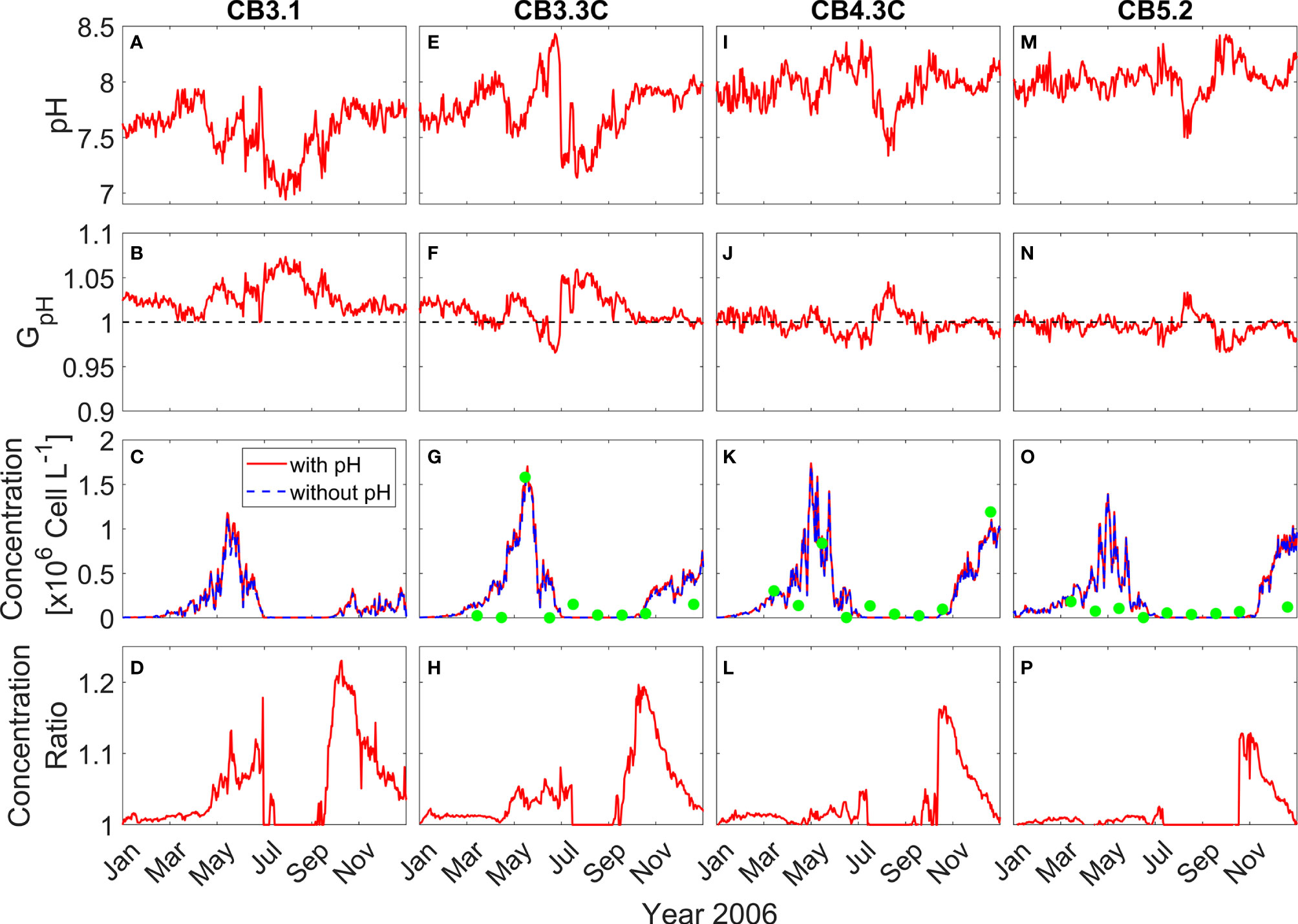
Figure 4 Time series of daily surface pH (A, E, I, M), G_pH (B, F, J, N), P. minimum cell concentration (C, G, K, O), and ratio of P. minimum concentration under pH effects to that without pH effects (D, H, L, P) in year 2006 at 4 mainstem stations marked in Figure 2A. Red solid lines represent the model results considering pH effects and blue dashed lines represent the model results without pH effects. Green dots represent the observed monthly mean P. minimum concentration.

At the mid bay station CB4.3C, surface pH generally increased from 7.9 to 8.2 between January and July (Figure 4I). It then dropped and reached the minimum (~ 7.5) in August and subsequently increased from September to December. The corresponding G_pH was slightly >1 during most of the time from January to May and then decreased to <1 in June and July (Figure 4J). G_pH increased to >1 in August and then decreased to slightly <1 again from September to December. Thus, surface P. minimum concentrations considering pH effects were also slightly higher than those without pH effects (Figure 4K), with the peak concentration during the spring bloom increasing by <5% (Figure 4L). At the lower bay station CB5.2, surface pH averaged around 8 and showed a weaker seasonal variation (Figure 4M). G_pH was slightly less than 1 all year except in August when pH reached the minimum (Figure 4N). There was virtually no difference in the cell density between the two model runs except in the late fall (Figures 4O, P). It was surprising to see higher P. minimum concentration at CB4.3C (4.2% increase) and CB5.2 (3.0% increase) during late fall when pH was high and G_pH < 1 (Figures 4J, N). On the other hand, P. minimum concentrations at the upper bay station CB3.1 remained elevated due to consistently low pH (Figure 4D). Seaward estuarine outflow could advect the higher biomass downstream, raising the cell density in the mid and lower bay even though the local growth rate was lower.

Focusing on the primary spring bloom period, monthly averaged surface pH in April increased from 7.7 in the upper bay to 8.0 in the mid bay while values were slightly lower, 7.9, in the lower bay (Figure 5A). G_pH was > 1 in the upper bay and < 1 in the mid-bay (Figure 5B). In the lower bay, G_pH was almost equal 1. Consequently P. minimum concentrations were moderately higher in the model run considering the pH effects (Figures 5C, D). In May, surface pH values in the mid bay and lower bay were similar to April, while the minimum surface pH in the upper bay declined to ~ 7.5 (Figure 5E). G_pH increased by 5% in the upper bay while dipping slight less than 1 in the mid-bay where pH remained above 8 (Figure 5F). The P. minimum bloom in May was mostly confined to the mid and upper bay, covering the mainstem between 38 and 39.2°N, as well as the Potomac River (Figure 5G). P. minimum concentrations increased everywhere in the bay, with the largest increase in the area between 38.7 and 39.3 °N (Figure 5H). The maximum increase in the cell density was 7 × 10⁴ cells L^-1 in the upper bay.

FIGURE 5

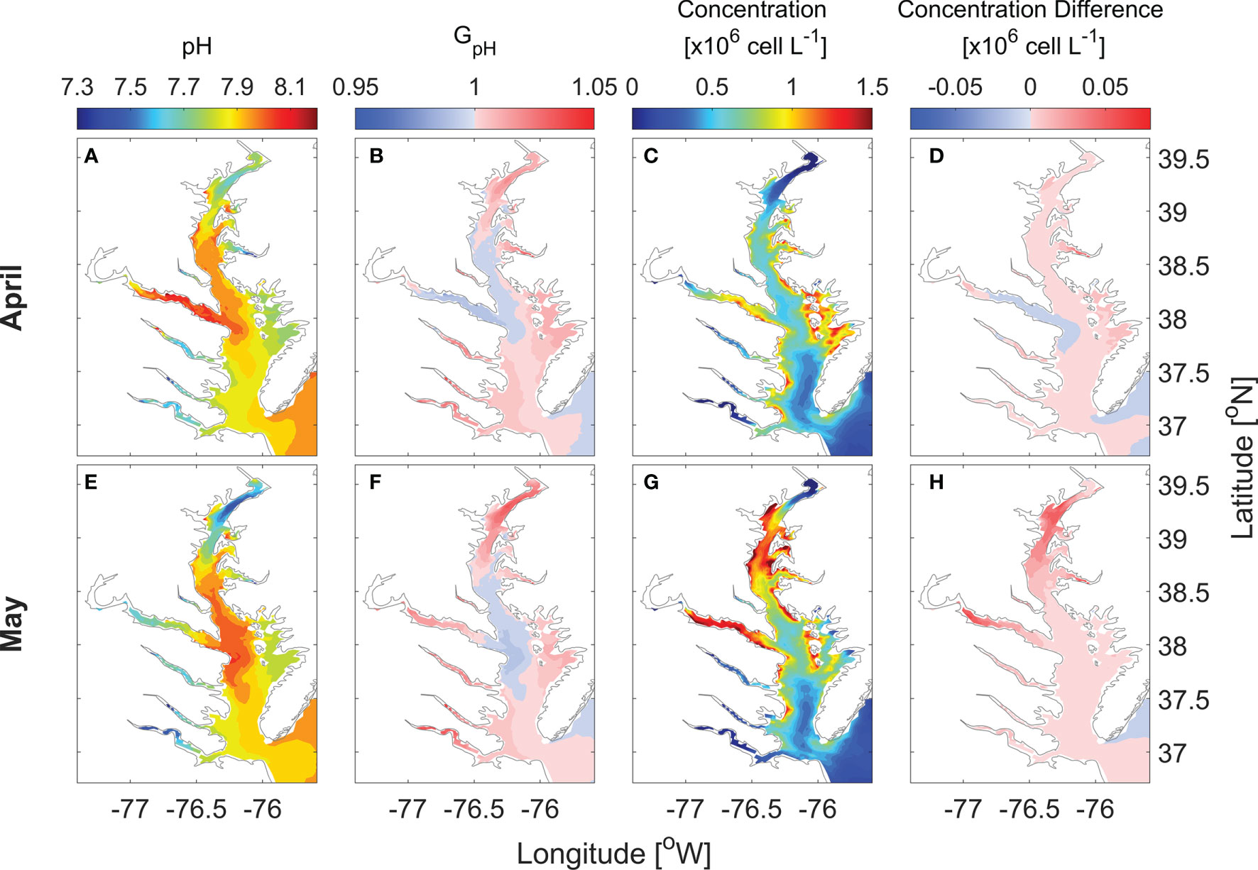
Figure 5 Horizontal distribution of monthly-mean surface pH (A, E), G_pH (B, F), P. minimum cell concentration (C, G) and the concentration difference between model with pH and without pH (D, H) in April and May when large blooms occurred in year 2006.

Along-channel distributions of pH, G_pH, and cell concentrations provide further information on the pH effects on the cell distributions (Figure 6). pH showed an along-channel gradient but also a vertical gradient, with the top-to-bottom difference reaching ~0.8 in the mid-bay (Figures 6A, E). G_pH of the bottom water was >1 due to lower pH (Figures 6B, F). In April, P. minimum concentrations were highest in the bottom waters of the lower bay as cells were advected landward by the estuarine return flow (Figure 6C). Since P. minimum growth was severely limited by light availability in the bottom waters, P. minimum concentrations did not increase despite the lower pH values (Figure 6D). In May, the bloom developed in the surface waters of the mid bay and upper bay (Figure 6G). Low pH in the upper bay enhanced G_pH (Figure 6F) and amplified the bloom size (Figure 6H). Although G_pH < 1 in the surface waters of the mid-bay, seaward advection of higher biomass from the upper bay compensated for the lower growth rate such that the P. minimum concentration in the mid-bay did not decrease (Figure 6H).

FIGURE 6

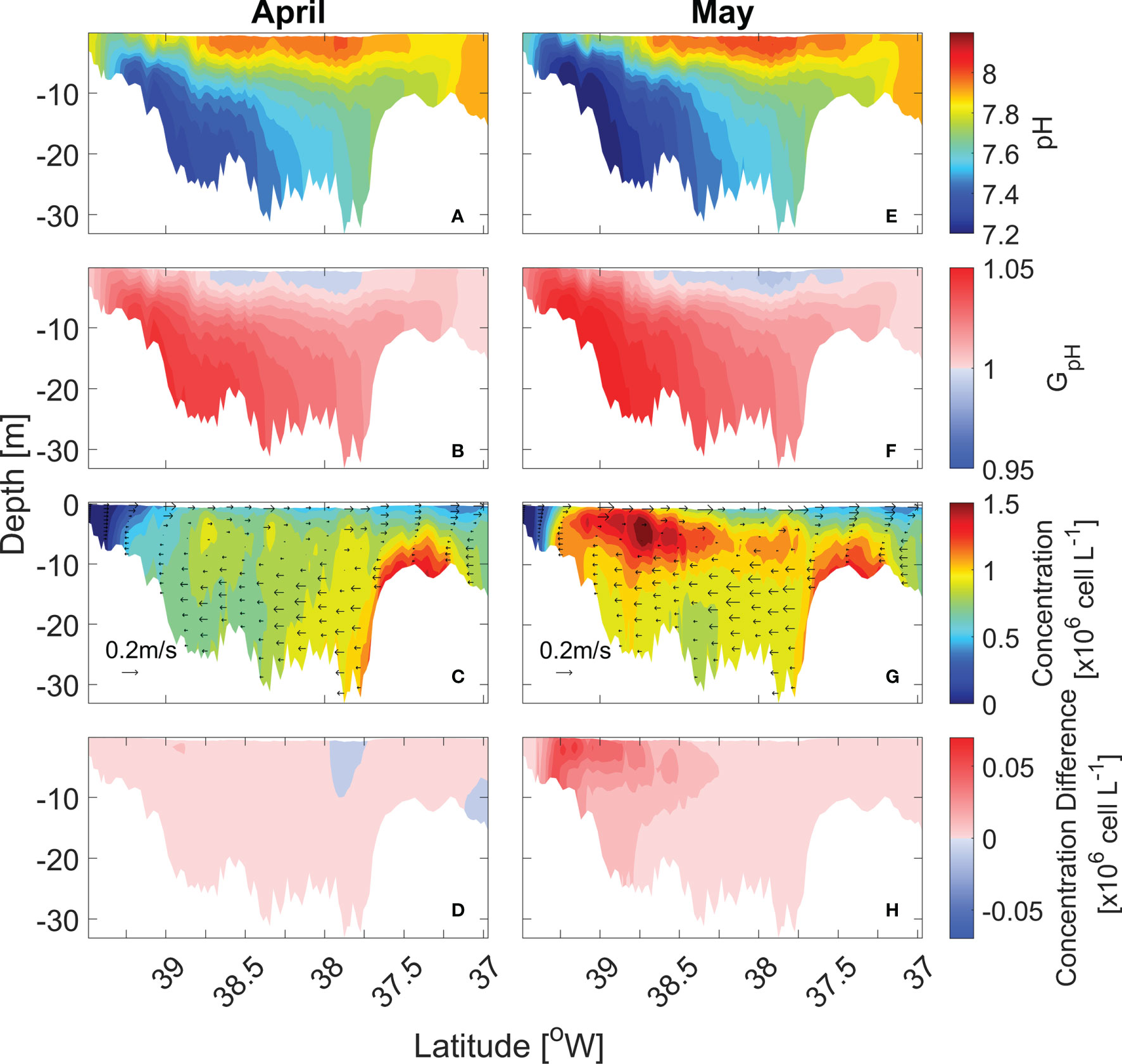
Figure 6 Along-channel distribution of monthly-mean pH (A, E), G_pH (B, F), P. minimum cell concentration (C, G) and the concentration difference between model with pH and without pH (D, H) in April and May in year 2006.

Projections for Effects of Future Acidification on P. minimum Bloom

To explore the impact of OA on P. minimum blooms in the future climate, the time series of the daily surface pH, pH decline, G_pH and P. minimum concentrations were compared for the years 2006, mid-21^st century 2050 and late-21^st century 2100 at the three stations (Figure 7). At the upper bay station CB3.1, pH is projected to decrease by ~0.1 in 2050 and ~0.2 in 2100 (Figures 7A, B). Correspondingly, G_pH time series shift upwards by ~0.007 in 2050 and ~0.015 in 2100 (Figure 7C). The averaged P. minimum concentrations in April and May increased 2.7% by 2050 and 5.5% by 2100 (Figure 7D). At the mid-bay station CB4.3C, pH shows a larger reduction, decreasing by ~0.15 in 2050 and ~0.3 in 2100 (Figures 7E, F). G_pH shifts upwards and remains > 1 all year in 2100 (Figure 7G). The average bloom size from April to June increases 2.0% in 2050 and 5.0% in 2100 (Figure 7H). pH reduction at the lower bay station CB5.2 is as large as that at CB4.3C (Figures 7I, J). In the mid- and late-21st century, G_pH is projected to stay above 1 during most of the year (Figure 7K). P. minimum concentrations during the spring blooms would increase 2.7% in 2050 and 5.3% in 2100 (Figure 7L). The time series of the concentration ratio between future scenarios and year 2006 show the same trend at the three stations. During the spring blooms, the percentage increase in P. minimum concentrations reaches a maximum in April, as pH decline is relatively larger (Figures 7B, F, G). It should also be noted that though the percentage increase in P. minimum concentrations during late fall is very large, the fall blooms are much smaller than the spring blooms.

FIGURE 7

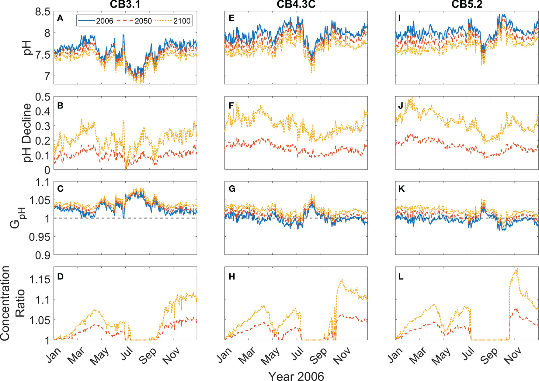
Figure 7 Time series of daily surface pH (A, E, I), pH decline (B, F, J), GpH (C, G, K), and ratio of P. minimum concentration in mid-21st century and late-21st century to that in year 2006 (D, H, L) at 3 mainstem stations marked in Figure 2A..

Surface distributions of monthly averaged pH, G_pH, and P. minimum concentrations in May are altered in the future scenario relative to the year 2006 (Figure 8). In 2050, monthly averaged surface pH in May ranges from 7.4 to 7.9, with an averaged decrease of ~ 0.1 as compared with year 2006 (Figure 8A). The area where G_pH is >1 would cover the whole bay (Figure 8B). Thus, P. minimum concentrations increase almost everywhere in the bay (Figure 8D). In 2100, monthly averaged surface pH in May decreases to 7.3 – 7.7 (Figure 8E). With such low pH, G_pH is even larger, reaching 1.05 in most area of the bay (Figure 8F). This results in even larger increases in P. minimum concentrations (Figure 8H).

FIGURE 8

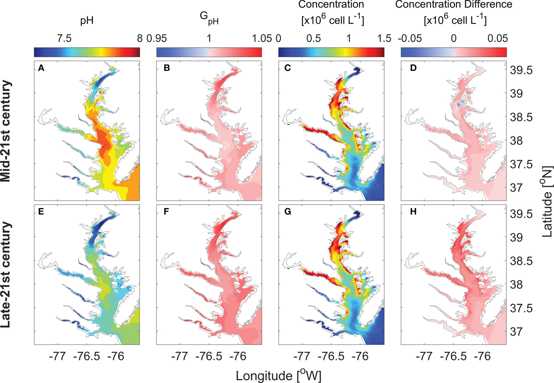
Figure 8 Horizontal distribution of monthly-mean surface pH (A, E), G_pH (B, F), P. minimum cell concentration (C, G), and the concentration difference between model results of future projection and year 2006 (D, H) in May.

Five stations were chosen to further illustrate the effects of OA on the peak bloom size of P. minimum (Figure 9). At the upper bay station CB3.1, the peak concentration increases 1.47% in the mid-21^st century and 2.86% in the late-21^st century as compared with the year 2006. Stations CB3.3C, CB4.1C, and CB4.3C are located in a region (38.5 – 39 °N) where the P. minimum blooms typically occur (Figure 5G). The peak P. minimum concentration at these three stations is projected to increase by 1.51%, 0.87%, 2.42% in 2050 and by 2.59%, 2.68%, 4.37% in 2100, respectively. At the station CB5.2 at the lower bay, the peak P. minimum concentration increases by 2.04% in 2050 and 3.73% in 2100.

FIGURE 9

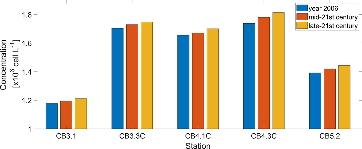
Figure 9 Comparison between peak P. minimum cell concentration during the spring bloom in May of year 2006, mid-21st century, and late-21st century at 5 mainstem stations marked in Figure 2A.

Discussion and Conclusion

Coupled hydrodynamic-carbonate chemistry–HAB models were developed to investigate the effects of OA on P. minimum blooms in Chesapeake bay. To our knowledge, this was the first attempt to couple 3D carbonate chemistry and HAB models for an estuarine region, representing a preliminary but an important step towards modeling and understanding the OA-HAB interactions in a changing climate. The model results showed a moderate effect of pH on P. minimum blooms but estuarine circulation transported P. minimum cells across large pH gradients in the estuary and produced unexpected changes in the bloom size across different parts of the estuary. For example, the estuarine outflow exported higher biomass in the low-pH upper bay to the mid- and lower bay where high pH suppresses P. minimum growth. The climate projections suggested 2.9% or 6.2% increase in the bay-averaged P. minimum concentration in 2050 or 2100 when the atmospheric pCO₂ increases to 550 or 800 ppm and pH in Chesapeake bay decreases by 0.2 or 0.4. This modest increase is consistent with laboratory results (Fu et al., 2008; Berge et al., 2010). It is possible some phytoplankton species like P. minimum are resistant to climate change in terms of OA as large pH fluctuations in space and time under the current climate make them capable of tolerating OA effects. Other species may show a stronger response. A recent meta-analysis of ~3000 studies on HABs globally reveals that the effects of elevated CO₂ on HAB growth rates varies both across and within species, but led to a significant overall increase in growth rate by 20% (Brandenburg et al., 2019). Our choice of P. minimum for this modeling study was driven by the availability of an existing mechanistic HAB model for Chesapeake bay. It is quite possible that a larger OA effect may be found for other HAB species and the modeling approach developed here can be readily extended to other HAB species in other estuaries or coastal oceans. The coupled carbonate chemistry and HAB models could also be extended to incorporate other effects of rising CO₂ on the HAB species as described below.

This modeling study focussed exclusively on the pH effects. However, previous studies suggested the potential effects of C limitation on algal growth under changing CO₂ conditions (e.g. Schippers et al., 2004; Almomani, 2019). In Chesapeake bay DIC ranges between 1000 and 2000 μM L^-1 under the current climate (Brodeur et al., 2019) and is expected to increase by 100-400 μM L^-1 in the 21^st century. Hence C limitation is not expected to be a major factor in P. minimum growth. Nevertheless, laboratory experiments showed that growth of species such as P. minimum may be affected by pH changes even when DIC limitation was minor (Hansen et al., 2007). The physiological responses of dinoflagellates to pH and CO₂ changes are likely complicated and future models need to take these processes into consideration. For example, elevated CO₂ could affect cellular quotas of C, N and P and the uptake rate of nutrients (Xia and Gao, 2005; Fu et al., 2007; Finkel et al., 2010). An increase of C:N or C:P could make the algae more prone to N-limitation or P-limitation, although elevated CO₂ did not significantly affect the elemental ratios of P. minimum (Fu et al., 2008).

The parameterization G_pH used in the HAB model (Eq. 2) was based on the laboratory experiments in which pH in the culture was altered through acid/base additions. Two approaches have been used to manipulate pH and the carbonate system in studies involving phytoplankton and responses to lowered pH and OA. One is based on acid/base additions and the other is CO₂ bubbling. The main difference lies in their different effects on the carbonate speciation, the total pool of inorganic C (TCO₂), and alkalinity of seawater medium (Berge et al., 2010). CO₂ bubbling leads to an increase in TCO₂ while alkalinity is kept constant and pH decreases. This reflects the changes related to ocean acidification due to increased atmospheric CO₂. In the HCl addition method, TCO₂ is kept stable while total alkalinity and pH decrease. There are heated discussions on which technique is most suitable for studying OA effects (Hurd et al., 2009; Schulz et al., 2009; Shi et al., 2009). The pros and cons of each technique make it more difficult to evaluate effects in estuarine and coastal environments where there are multiple sources of inorganic C (e.g. riverine inputs, oceanic import, uptake from the atmosphere, respiration of organic matter). Future modeling development for studying OA-HAB interaction requires a close integration between the experimental and modeling approaches.

To investigate the influence of future acidification on P. minimum blooms, two scenario runs were conducted under the elevated pCO₂ conditions projected for the mid- and late-21^st century conditions. However, these model runs did not consider all climate-change impacts on Chesapeake bay such as warming, sea level rise and altered river flows (Ni et al., 2019). In their laboratory experiments, Fu et al. (2008) found raising CO₂ alone increased the growth rate of P. minimum but higher CO₂ and warming in combination did not produce significant change on P. minimum growth. A future modeling study needs to consider these combined effects (e.g., Glibert, 2020). Previous projections of P. minimum in Chesapeake bay, based on a habitat model, showed that P. minimum biomass may shift upstream due to salinity changes caused by sea level rise and changes in the river flow (Li et al., 2020b). As the biomass in the upper bay increases, the low-pH water there may lead to a larger increase in P. minimum concentration and the estuarine outflow may transport these cells downstream. Furthermore, reduced pH could increase the toxicity of some harmful algae (Sun et al., 2011; Tatters et al., 2012). While the toxicity of P. minimum in Chesapeake bay has not been documented, and the toxicity of this species is a topic of debate (Heil et al., 2005), the harm to estuarine ecology could be much larger under elevated pCO₂ for related toxic HAB taxa.

It is also worth noting that this model does not consider the complexity of mixotrophic nutrition of P. minimum and how that may change under altered CO₂ conditions. Indeed, for this first effort of coupling the carbon chemistry model with the HAB model, a species that does not have strong dependence on mixotrophy was purposely chosen. A three-dimensional mixotrophic model for a different HAB taxon of Chesapeake bay, Karlodinium veneficum, has recently been developed (Li et al., 2022), and the aim is to couple this complex HAB model to the ROMS-RCA-CC model in the future.

Data Availability Statement

Model results in this study can be downloaded from https://zenodo.org/record/6318647#.Yh274OjMKUk.

Author Contributions

ML, PG, and RL conceived the ideas. RL configured the model and conducted the numerical simulations. RL and ML analyzed the model results. RL wrote the paper with editorial contributions from ML and PG. All authors contributed to the article and approved the submitted version.

Funding

We are grateful to the National Oceanic and Atmospheric Administration National Centers for Coastal Ocean Science Competitive Research Program under award NA17NOS4780180 to UMCES for the financial support.

Conflict of Interest

The authors declare that the research was conducted in the absence of any commercial or financial relationships that could be construed as a potential conflict of interest.

Publisher’s Note

All claims expressed in this article are solely those of the authors and do not necessarily represent those of their affiliated organizations, or those of the publisher, the editors and the reviewers. Any product that may be evaluated in this article, or claim that may be made by its manufacturer, is not guaranteed or endorsed by the publisher.

Acknowledgments

We thank three reviewers for their helpful comments. This is ECOHAB contribution number 1024 and contribution number 6186 from the University of Maryland Center for Environmental Science.

References

Almomani F. A. (2019). Assessment and Modeling of Microalgae Growth Considering the Effects OF CO₂, Nutrients, Dissolved Organic Carbon and Solar Irradiation. J.Env. Manage. 247, 738–748. doi: 10.1016/j.jenvman.2019.06.085

CrossRef Full Text | Google Scholar

Bakker D. C. E., Pfeil B., Landa C. S., Metzl N., O’Brien K. M., Olsen A., et al. (2016). A Multi-Decade Record of High-Quality fCO₂ Data in Version 3 of the Surface Ocean CO₂ Atlas (SOCAT). Earth Syst. Sci. Data 8, 383–413. doi: 10.5194/essd-8-383-2016

CrossRef Full Text | Google Scholar

Bates N. R., Astor Y., Church M., Currie K., Dore J., González-Dávila M., et al. (2014). A Time-Series View of Changing Ocean Chemistry Due to Ocean Uptake of Anthropogenic CO₂ and Ocean Acidification. Oceanography 27 (1), 126–141. doi: 10.5670/oceanog.2014.16

CrossRef Full Text | Google Scholar

Beardall J., Raven J. A. (2004). The Potential Effects of Global Climate Change on Microbial Photosynthesis, Growth and Ecology. Phycologia 43, 26–40. doi: 10.2216/i0031-8884-43-1-26.1

CrossRef Full Text | Google Scholar

Beardall J., Stojkovic S., Larsen S. (2009). Living in a High CO₂ World: Impacts of Global Climate Change on Marine Phytoplankton. Plant Ecol. Diver. 2 (2), 191–205. doi: 10.1080/17550870903271363

CrossRef Full Text | Google Scholar

Berge T., Daugbjerg N., Andersen B. B., Hansen P. J. (2010). Effect of Lowered pH on Marine Phytoplankton Growth Rates. Mar. Ecol. Prog. Ser. 416, 79–91. doi: 10.3354/meps08780

CrossRef Full Text | Google Scholar

Brady D. C., Testa J. M., Di Toro D. M., Boynton W. R., Kemp W. M. (2013). Sediment Flux Modeling: Calibration and Application for Coastal Systems. Est. Coast. Shelf. Sci. 117, 107–124. doi: 10.1016/j.ecss.2012.11.003

CrossRef Full Text | Google Scholar

Brandenburg K. M., Velthuis M., Van de Waal D. B. (2019). Meta-Analysis Reveals Enhanced Growth of Marine Harmful Algae From Temperate Regions With Warming and Elevated CO₂ Levels. Glob. Change Biol. 25 (8), 2607–2618. doi: 10.1111/gcb.14678

CrossRef Full Text | Google Scholar

Brodeur J. R., Chen B., Zhong J., Xu Y., Hussain N., Scaboo K. M., et al. (2019). Chesapeake bay Inorganic Carbon, Spatial Distribution and Seasonal Variability. Front. Mar. Sci. 6. doi: 10.3389/fmars.2019.00099

CrossRef Full Text | Google Scholar

Cai W., Feely R. A., Testa J. M., Li M., Evans W., Alin S. R., et al. (2021). Natural and Anthropogenic Drivers of Acidification in Large Estuaries. Annu. Rev. Mar. Sc. 13, pp.23–pp.55. doi: 10.1146/annurev-marine-010419-011004

CrossRef Full Text | Google Scholar

Cai W., Huang W., Luther G. W., Pierrot D., Li M., Testa J. M., et al. (2017). Redox Reactions and Weak Buffering Capacity Lead to Acidification in the Chesapeake bay. Nat. Commun. 8, 369. doi: 10.1038/s41467-017-00417-7

PubMed Abstract | CrossRef Full Text | Google Scholar

Cai W.-J., Hu X., Huang W.-J., Jiang L.-Q., Wang Y., Peng T. H., et al. (2010). Alkalinity Distribution in the Western North Atlantic Ocean Margins. J. Geophys. Res. Ocean. 115, C08014. doi: 10.1029/2009JC005482

CrossRef Full Text | Google Scholar

Cai W., Hu X., Huang W., Murrell M. C., Lehrter J. C., Lohrenz S. E., et al. (2011). Acidification of Subsurface Coastal Waters Enhanced by Eutrophication. Nat. Geosci. 4, 766–770. doi: 10.1038/ngeo1297

CrossRef Full Text | Google Scholar

Chen B., Cai W.-J., Brodeur J. R., Hussain N., Testa J. M., Ni W., et al. (2020). Seasonal and Spatial Variability in Surface pCO₂ and Air-Water CO₂ Flux in the Chesapeake bay. Limnol. Oceanogr. 65 (12), 3046–3065. doi: 10.1002/lno.11573

CrossRef Full Text | Google Scholar

Da F., Friedrichs M. A., St-Laurent P., Shadwick E. H., Najjar R. G., Hinson K. E. (2021). Mechanisms Driving Decadal Changes in the Carbonate System of a Coastal Plain Estuary. J. Geophys. Res. Ocean. 126 (6), e2021JC017239. doi: 10.1029/2021JC017239

CrossRef Full Text | Google Scholar

Di Toro D. M. (2001). Sediment Flux Modeling (New York, NY: Wiley-Interscience).

Google Scholar

Doney S. C., Busch D. S., Cooley S. R., Kroeker K. J. (2020). The Impacts of Ocean Acidification on Marine Ecosystems and Reliant Human Communities. Annu. Rev. Environ. Resour. 45, 83–112. doi: 10.1146/annurev-environ-012320-083019

CrossRef Full Text | Google Scholar

Doney S. C., Ruckelshaus M., Duffy J. E., Barry J. P., Chan F., English C. V. A., et al. (2012). Climate Change Impacts on Marine Ecosystems. Annu. Rev. Mar. Sc. 4, 11–37. doi: 10.1146/annurev-marine-041911-111611

CrossRef Full Text | Google Scholar

Egbert G. D., Erofeeva S. Y. (2002). Efficient Inverse Modeling of Barotropic Ocean Tides. J. Atmos. Ocean. Tech. 19 (2), 183–204. doi: 10.1175/1520-0426(2002)019<0183:eimobo>2.0.co;2

CrossRef Full Text | Google Scholar

Feely R. A., Doney S. C., Cooley S. R. (2009). Ocean Acidification: Present Conditions and Future Changes in a High CO₂ World. Oceanography 22 (4), 36–47. doi: 10.5670/oceanog.2009.95

CrossRef Full Text | Google Scholar

Feely R. A., Sabine C. L., Lee K., Berelson W., Kleypas J., Fabry V. J., et al. (2004). Impact of Anthropogenic CO₂ on the CaCO₃ System in the Oceans. Science 305 (5682), 362–366. doi: 10.1126/science.1097329

PubMed Abstract | CrossRef Full Text | Google Scholar

Filippino K. C., Mulholland M. R., Bernhardt P. W. (2011). Nitrogen Uptake and Primary Productivity Rates in the Mid-Atlantic Bight (MAB). Estuar. Coast. Shelf. Sci. 91, 13–23. doi: 10.1016/j.ecss.2010.10.001

CrossRef Full Text | Google Scholar

Finkel Z. V., Beardall J., Flynn K. J., Quigg A., Rees T. A. V., Raven J. A. (2010). Phytoplankton in a Changing World: Cell Size and Elemental Stoichiometry. J. Plankt. Res. 32, 119–137. doi: 10.1093/plankt/fbp098

CrossRef Full Text | Google Scholar

Flynn K. J., Clark D. R., Mitra A., Fabian H., Hansen P. J., Glibert P. M., et al. (2015). Ocean Acidification With (De) Eutrophication Will Alter Future Phytoplankton Growth and Succession. Proc. R. Soc B.: Biol. Sci. 282 (1804), 20142604. doi: 10.1098/rspb.2014.2604

CrossRef Full Text | Google Scholar

Friedman J. R., Shadwick E. H., Friedrichs M. A. M., Najjar R. G., De Meo O. A., Da F., et al. (2020). Seasonal Variability of the CO₂ System in a Large Coastal Plain Estuary. J. Geophys. Res. Ocean. 125, e2019JC015609. doi: 10.1029/2019JC015609

CrossRef Full Text | Google Scholar

Fu F.-X., Warner M., Zhang Y., Feng Y., Hutchins D. A. (2007). Effects of Increased Temperature and CO₂ on Photosynthesis, Growth and Elemental Ratios in the Marine Cyanobacteria Synechococcus and Prochlorococcus. J. Phycol. 43, 485–496. doi: 10.1111/j.1529-8817.2007.00355.x

CrossRef Full Text | Google Scholar

Fu F. X., Zhang Y., Warner M. E., Feng Y., Sun J., Hutchins D. A. (2008). A Comparison of Future Increased CO₂ and Temperature Effects on Sympatric Heterosigma Akashiwo and Prorocentrum Minimum. Harmf. Algae. 7 (1), 76–90. doi: 10.1016/j.hal.2007.05.006

CrossRef Full Text | Google Scholar

Giordano M., Beardall J., Raven J. A. (2005). CO₂ Concentrating Mechanisms in Algae: Mechanisms, Environmental Modulation, and Evolution. Annu. Rev. Plant Biol. 56, 99–131. doi: 10.1146/annurev.arplant.56.032604.144052

PubMed Abstract | CrossRef Full Text | Google Scholar

Glibert P. M. (2020). Harmful Algal at the Complex Nexus of Eutrophication and Climate Change. Harmf. Algae. 91, 101583. doi: 10.1016/j.hal.2019.03.001

CrossRef Full Text | Google Scholar

Glibert P. M., Burford M. A. (2017). Globally Changing Nutrient Loads and Harmful Algal Blooms: Recent Advances, New Paradigms and Continuing Challenges. Oceanography 30 (1), 44–55. doi: 10.5670/oceanog.2017.110

CrossRef Full Text | Google Scholar

Glibert P. M., Burkholder J. M., Kana T. M. (2012). Recent Insights About Relationships Between Nutrient Availability, Forms, and Stoichiometry, and the Distribution, Ecophysiology, and Food Web Effects of Pelagic and Benthic Prorocentrum Species. Harmf. Algae. 14, 231–259. doi: 10.1016/j.hal.2011.10.023

CrossRef Full Text | Google Scholar

Glibert P. M., Mayorga E., Seitzinger S. (2008). Prorocentrum Minimum Tracks Anthropogenic Nitrogen and Phosphorus Inputs on a Global Basis: Application of Spatially Explicit Nutrient Export Models. Harmf. Algae. 8 (1), 33–38. doi: 10.1016/j.hal.2008.08.023

CrossRef Full Text | Google Scholar

Haidvogel D. B., Arango H., Budgell W. P., Cornuelle B. D., Curchitser E., Di Lorenzo E., et al. (2008). Ocean Forecasting in Terrain-Following Coordinates: Formulation and Skill Assessment of the Regional Ocean Modeling System. J. Comput. Phys. 227, 3595–3624. doi: 10.1016/j.jcp.2007.06.016

CrossRef Full Text | Google Scholar

Hansen P. J. (2002). Effect of High pH on the Growth and Survival of Marine Phytoplankton: Implications for Species Succession. Aquat. Microb. Ecol. 28, 279–288. doi: 10.3354/ame028279

CrossRef Full Text | Google Scholar

Hansen P. J., Lundholm N., Rost B. (2007). Growth Limitation in Marine Red-Tide Dinoflagellates: Effects of pH Versus Inorganic Carbon Availability. Mar. Ecol. Prog. Ser. 334, 63–71. doi: 10.3354/meps334063

CrossRef Full Text | Google Scholar

Heil C. A., Glibert P. M., Fan C. (2005). Prorocentrum Minimum (Pavillard) Schiller: A Review of a Harmful Algal Bloom Species of Growing Worldwide Importance. Harmf. Algae. 4 (3), 449–470. doi: 10.1016/j.hal.2004.08.003

CrossRef Full Text | Google Scholar

Huang W.-J., Cai W.-J., Xie X., Li M. (2019). Wind-Driven Lateral Variations of Partial Pressure of Carbon Dioxide in a Large Estuary. J. Mar. Syst. 195, 67–73. doi: 10.1016/j.jmarsys.2019.03.002

CrossRef Full Text | Google Scholar

Hurd C. L., Hepburn C. D., Currie K. I., Raven J. A., Hunter K. A. (2009). Testing the Effects of Ocean Acidification on Algal Metabolism: Considerations for Experimental Designs. J. Phycol. 45, 1236–1251. doi: 10.1111/j.1529-8817.2009.00768.x

PubMed Abstract | CrossRef Full Text | Google Scholar

IPCC (2021). “Climate Change 2021: The Physical Science Basis,” in Contribution of Working Group I to the Sixth Assessment Report of the Intergovernmental Panel on Climate Change (Cambridge, United Kingdom and New York, NY, USA: Cambridge University Press). doi: 10.1017/9781009157896

CrossRef Full Text | Google Scholar

Isleib R. P. E., Fitzpatrick J. J., Mueller J. (2007). The Development of a Nitrogen Control Plan for a Highly Urbanized Tidal Embayment. Proc. Water Environ. Feder. 5, 296–320. doi: 10.2175/193864707786619152

CrossRef Full Text | Google Scholar

Jiang L.-Q., Carter B. R., Feely R. A., Lauvset S. K., Olsen A. (2019). Surface Ocean pH and Buffer Capacity: Past, Present and Future. Sci. Rep. 9, 18624. doi: 10.1038/s41598-019-55039-4

PubMed Abstract | CrossRef Full Text | Google Scholar

Kaushal S. S., Likens G. E., Utz R. M., Pace M. L., Grese M., Yepsen M. (2013). Increased River Alkalinization in the Eastern U.S. Environ. Sci. Technol. 47, 10,302–10,311. doi: 10.1021/es401046s

CrossRef Full Text | Google Scholar

Lewis E. R., Wallace D. W. R. (1998). CO2SYS-Program Developed for CO₂ System Calculations (Tennessee: Carbon Dioxide Inf. Anal. Centre).

Google Scholar

Li J., Glibert P. M., Gao Y. (2015). Temporal and Spatial Changes in Chesapeake bay Water Quality and Relationships to Prorocentrum Minimum, Karlodinium Veneficum, and CyanoHAB Event, 1991–2008. Harmf. Algae. 42, 1–14. doi: 10.1016/j.hal.2014.11.003

CrossRef Full Text | Google Scholar

Li M., Lee Y. J., Testa J. M., Li Y., Ni W., Kemp W. M., et al. (2016). What Drives Interannual Variability of Hypoxia in Chesapeake bay: Climate Forcing Versus Nutrient Loading? Geophys. Res. Lett. 43, 2127–2134. doi: 10.1002/2015GL067334

CrossRef Full Text | Google Scholar

Li M., Li R., Cai W.-J., Testa J. M., Shen C. (2020a). Effects of Wind-Driven Lateral Upwelling on Estuarine Carbonate Chemistry. Front. Mar. Sci 7. doi: 10.3389/fmars.2020.588465

CrossRef Full Text | Google Scholar

Li M., Ni W., Zhang F., Glibert P. M., Lin C.-H. (2020b). Climate-Induced Interannual Variability and Projected Change of Two Harmful Algal Bloom Taxa in Chesapeake bay. USA. Sci. Tot. Environ. 744, 140947. doi: 10.1016/j.scitotenv.2020.140947

CrossRef Full Text | Google Scholar

Li M., Zhang F., Glibert P. M. (2021). Seasonal Life Strategy of Prorocentrum Minimum in Chesapeake bay, USA: Validation of the Role of Physical Transport Using a Coupled Physical–Biogeochemical–Harmful Algal Bloom Model. Limnol. Oceanogr. 66 (11), 3873–3886. doi: 10.1002/lno.11925

CrossRef Full Text | Google Scholar

Li M., Zhong L., Boicourt W. C. (2005). Simulations of Chesapeake bay Estuary: Sensitivity to Turbulence Mixing Parameterizations and Comparison With Observations. J. Geophys. Res. Ocean. 110, C12004. doi: 10.1029/2004JC002585

CrossRef Full Text | Google Scholar

Li M., Zhang F., Glibert P. M. (2021). Seasonal Life Strategy of Prorocentrum Minimum in Chesapeake bay, USA: Validation of the Role of Physical Transport Using a Coupled Physical–Biogeochemical–Harmful Algal Bloom Model. Limnol. Oceanogr. 66 (11), 3873–3886. doi: 10.1002/lno.11925

CrossRef Full Text | Google Scholar

Li M., Chen Y., Zhang F., Song Y., Glibert P.M., Stoecker D.K., et al. (2022). A Three-dimensional Mixotrophic Model of Karlodinium Veneficum Blooms for a Eutrophic Estuary. Harmf. Algae 113, 102203. doi: 10.1016/j.hal.2022.102203

CrossRef Full Text | Google Scholar

Ni W., Li M., Ross A. C., Najjar R. G. (2019). Large Projected Decline in Dissolved Oxygen in a Eutrophic Estuary Due to Climate Change. J. Geophys. Res. Ocean. 124 (11), 8271–8289. doi: 10.1029/2019JC015274

CrossRef Full Text | Google Scholar

Ni W., Li M., Testa J. M. (2020). Discerning Effects of Warming, Sea Level Rise and Nutrient Management on Long-Term Hypoxia Trends in Chesapeake bay. Sci. Tot. Envir. 737, 139717. doi: 10.1016/j.scitotenv.2020.139717

CrossRef Full Text | Google Scholar

O'Neil J. M., Davis T. W., Burford M. A., Gobler C. A. (2012). The Rise of Harmful Cyanobacteria Blooms: The Potential Roles of Eutrophication and Climate Change. Harmf. Algae. 14, 313–334. doi: 10.1016/j.hal.2011.10.027

CrossRef Full Text | Google Scholar

Paerl H. W., Huisman J. (2008). Blooms Like it Hot. Science 320, 57–58. doi: 10.1126/science.1155398

PubMed Abstract | CrossRef Full Text | Google Scholar

Raven J. A., Beardall J. (2014). CO₂ Concentrating Mechanisms and Environmental Change. Aquat. Bot. 118, 24–37. doi: 10.1016/j.aquabot.2014.05.008

CrossRef Full Text | Google Scholar

Raymond P. A., Bauer J. E., Cole J. J. (2000). Atmospheric CO₂ Evasion, Dissolved Inorganic Carbon Production, and Net Heterotrophy in the York River Estuary. Limnol. Oceanogr. 45, 1707–1717. doi: 10.4319/lo.2000.45.8.1707

CrossRef Full Text | Google Scholar

Rost B., Riebesell U., Burkhardt S., Sultemeyer D. (2003). Carbon Acquisition of Bloom-Forming Marine Phytoplankton. Limnol. Oceanogr. 48 (1), 55–67. doi: 10.4319/lo.2003.48.1.0055

CrossRef Full Text | Google Scholar

Schippers P., Lurling M., Scheffer M. (2004). Increase of Atmospheric CO₂ Promotes Phytoplankton Productivity. Ecol. Lett. 7, 446–451. doi: 10.1111/j.1461-0248.2004.00597.x

CrossRef Full Text | Google Scholar

Schulz K. G., Barcelos e Ramos J., Zeebe R. E., Riebesell U. (2009). CO2 Perturbation Experiments: Similarities and Differences Between Dissolved Inorganic Carbon and Total Alkalinity Manipulations. Biogeosciences 6, 2145–2153. doi: 10.5194/bg-6-2145-2009

CrossRef Full Text | Google Scholar

Shadwick E. H., Friedrichs M. A. M., Najjar R. G., De Meo O. A., Friedman J. R., Da F., et al. (2019). High Frequency CO₂ System Variability Over the Winter-to-Spring Transition in a Coastal Plain Estuary. J. Geophys. Res. Ocean. 124, 7626–7642. doi: 10.1029/2019JC015246

CrossRef Full Text | Google Scholar

Shchepetkin A. F., McWilliams J. C. (2005). The Regional Oceanic Modeling System (ROMS): A Split-Explicit, Free-Surface, Topography-Following-Coordinate Oceanic Model. Ocean. Model. 9, 347–404. doi: 10.1016/j.ocemod.2004.08.002

CrossRef Full Text | Google Scholar

Shen C., Testa J. M., Li M., Cai W.-J. (2020). Understanding Anthropogenic Impacts on pH and Aragonite Saturation State in Chesapeake bay: Insights From a 30-Year Model Study. J. Geophys. Res. Biogeosci. 125, e2019JG005620. doi: 10.1029/2019JG005620

CrossRef Full Text | Google Scholar

Shen C., Testa J. M., Li M., Cai W.-J., Waldbusser G. G., Ni W., et al. (2019a). Controls on Carbonate System Dynamics in a Coastal Plain Estuary: A Modeling Study. J. Geophys. Res. Biogeosci. 124, 61–78. doi: 10.1029/2018JG004802

CrossRef Full Text | Google Scholar

Shen C., Testa J. M., Ni W., Cai W.-J., Li M., Kemp W. M. (2019b). Ecosystem Metabolism and Carbon Balance in Chesapeake bay: A 30-Year Analysis Using a Coupled Hydrodynamic-Biogeochemical Model. J. Geophys. Res. Ocean. 124, 6141–6153. doi: 10.1029/2019jc015296

CrossRef Full Text | Google Scholar

Shi D., Xu Y., Hopkinson B. M., Morel F. M. M. (2010). Effect of Ocean Acidification on Iron Availability to Marine Phytoplankton. Science 327 (5966), 676–679. doi: 10.1126/science.1183517

PubMed Abstract | CrossRef Full Text | Google Scholar

Shi D., Xu Y., Morel F. M. M. (2009). Effects of the pH/pCO₂ Control Method on Medium Chemistry and Phytoplankton Growth. Biogeosciences 6, 1199–1207. doi: 10.5194/bg-6-1199-2009

CrossRef Full Text | Google Scholar

Su J., Cai W. J., Brodeur J., Chen B., Hussain N., Yao Y., et al. (2020). Chesapeake bay Acidification Buffered by Spatially Decoupled Carbonate Mineral Cycling. Nat. Geosci. 13 (6), 441–447. doi: 10.1038/s41561-020-0584-3

CrossRef Full Text | Google Scholar

Su J., Cai W. J., Testa J. M., Brodeur J. R., Chen B., Scaboo K. M., et al. (2021). Supply-Controlled Calcium Carbonate Dissolution Decouples the Seasonal Dissolved Oxygen and pH Minima in Chesapeake bay. Limnol. Oceanogr. 66 (10), 3796–3810. doi: 10.1002/lno.11919

CrossRef Full Text | Google Scholar

Sun J., Hutchins D. A., Feng Y. Y., Seubert E. L., Caron D. A., Fu F. X. (2011). Effects of Changing pCO₂ and Phosphate Availability on Domoic Acid Production and Physiology of the Marine Harmful Bloom Diatom. Pseudo-nitzschia. Multiseries. Limnol. Oceanogr. 56 (3), 829–840. doi: 10.4319/lo.2011.56.3.0829

CrossRef Full Text | Google Scholar

Takahashi T., Sutherland S. C., Chipman D. W., Goddard J. G., Ho C., Newberger T., et al. (2014). Climatological Distributions of Ph, pCO₂, Total CO₂, Alkalinity, and CaCO₃ Saturation in the Global Surface Ocean, and Temporal Changes at Selected Locations. Mar. Chem. 164, 95–125. doi: 10.1016/j.marchem.2014.06.004

CrossRef Full Text | Google Scholar

Tango P. J., Magnien R., Butler W., Luckett C., Luckenbach M., Lacouture R., et al. (2005). Impacts and Potential Effects Due to Prorocentrum minimum Blooms in Chesapeake bay. Harmf. Algae. 4, 525–531. doi: 10.1016/j.hal.2004.08.014

CrossRef Full Text | Google Scholar

Tatters A. O., Fu F. X., Hutchins D. A. (2012). High CO₂ and Silicate Limitation Synergistically Increase the Toxicity of Pseudo-Nitzshia Fraudulenta. PloS One 7 (2), e32116. doi: 10.1371/journal.pone.0032116

PubMed Abstract | CrossRef Full Text | Google Scholar

Testa J. M., Brady D. C., Di Toro D. M., Boynton W. R., Cornwell J. C., Kemp W. M. (2013). Sediment Flux Modeling: Nitrogen, Phosphorus and Silica Cycles. Estuar. Coast. Shelf. Sci. 131, 245–263. doi: 10.1016/j.ecss.2013.06.014

CrossRef Full Text | Google Scholar

Testa J. M., Li Y., Lee Y. J., Li M., Brady D. C., Di D. M., et al. (2014). Quantifying the Effects of Nutrient Loading on Dissolved O₂ Cycling and Hypoxia in Chesapeake bay Using a Coupled Hydrodynamic – Biogeochemical Model. J. Mar. Syst. 139, 139–158. doi: 10.1016/j.jmarsys.2014.05.018

CrossRef Full Text | Google Scholar

Testa J. M., Li Y., Lee Y. J., Li M., Brady D. C., DiToro D. M., et al. (2017). “Modeling Physical and Biogeochemical Controls on Dissolved Oxygen in Chesapeake bay: Lessons Learned From Simple and Complex Approaches,” in Modeling Coastal Hypoxia - Numerical Simulations of Patterns, Controls and Effects of Dissolved Oxygen Dynamics. Eds. Justic D., Rose K., Hetland R., Fennel K. (Switzerland: Springer), 95–118. doi: 10.1007/978-3-319-54571-4_5

CrossRef Full Text | Google Scholar

Tortell P. D. (2000). Evolutionary and Ecological Perspectives on Carbon Acquisition in Phytoplankton. Limnol. Oceanogr. 45 (3), 744–750. doi: 10.4319/lo.2000.45.3.0744

CrossRef Full Text | Google Scholar

Tyler M. A., Seliger H. H. (1978). Annual Subsurface Transport of a Red Tide Dinoflagellate to its Bloom Area: Water Circulation Patterns and Organism Distributions in the Chesapeake bay 1. Limnol. Oceanogr. 23 (2), pp.227–pp.246. doi: 10.4319/lo.1978.23.2.0227

CrossRef Full Text | Google Scholar

Wells M. L., Trainer V. L., Smayda T. J., Karlson B. S., Trick C. G., Kudela R. M., et al. (2015). Harmful Algal Blooms and Climate Change: Learning From the Past and Present to Forecast the Future. Harmf. Algae. 49, 68–93. doi: 10.1016/j.hal.2015.07.009

CrossRef Full Text | Google Scholar

Xia J.-R., Gao K.-S. (2005). Impacts of Elevated CO₂ Concentration on Biochemical Composition, Carbonic Anhydrase, and Nitrate Reductase Activity of Freshwater Green Algae. J. Int. Plant Biol. 47, 668–675. doi: 10.1111/j.1744-7909.2005.00114.x

CrossRef Full Text | Google Scholar

Xie X., Li M. (2018). Effects of Wind Straining on Estuarine Stratification: A Combined Observational and Modeling Study. J. Geophys. Res. Ocean. 123, 2363–2380. doi: 10.1002/2017JC013470

CrossRef Full Text | Google Scholar

Xie X., Li M. (2019). Generation of Internal Lee Waves by Lateral Circulation in a Coastal Plain Estuary. J. Phys. Oceanogr. 49 (7), 1687–1697. doi: 10.1175/JPO-D-18-0142.1

CrossRef Full Text | Google Scholar

Zhang F., Li M., Glibert P. M., Ahn S. H. S. (2021). A Three-Dimensional Mechanistic Model of Prorocentrum Minimum Blooms in Eutrophic Chesapeake bay. Sci. Tot. Environ. 769, 144528. doi: 10.1016/j.scitotenv.2020.144528

CrossRef Full Text | Google Scholar

Zhong L., Li M. (2006). Tidal Energy Fluxes and Dissipation in the Chesapeake bay. Cont. Shelf. Res. 26, 752–770. doi: 10.1016/j.csr.2006.02.006

CrossRef Full Text | Google Scholar

Zhong L., Li M., Foreman M. G. (2008). Resonance and Sea Level Variability in Chesapeake bay. Cont. Shelf. Res. 28, 2565–2573. doi: 10.1016/j.csr.2008.07.007

CrossRef Full Text | Google Scholar