Compound Effects of Flood Drivers, Sea Level Rise, and Dredging Protocols on Vessel Navigability and Wetland Inundation Dynamics

1 Introduction

Maritime transportation (MT) is considered the most cost-effective alternative for movement of freight as it takes advantage of intercontinental routes that connect ports and harbors around the globe. MT supports trade relations and contributes to local and regional economic development via global supply chains (Carse and Lewis, 2020). It has been reported that international marine trade by cargo increased from 4k to 12k million tons between 1970 and 2018 (UNCTAD, 2019), and recent estimates indicate that MT accounts for 90% of global trade in terms of volume (Rodrigue, 2020). With the expansion of the Panama Canal in 2016, port authorities have been upgrading existing marine infrastructure (e.g., ports, terminals, and docks) to accommodate deep draft-vessels navigating the Atlantic Ocean and the Pacific Ocean. Specifically, port authorities are targeting the new-class of ‘Neopanamax’ vessels that are 1200 ft long (~366 m), 168 ft wide (~49 m), have a 50 ft draft (~15 m), and can transport twice the cargo load p12.5k twenty-foot equivalent unit (TEU)] of the former standard ‘Panamax’ vessel (Medina et al., 2020; Rodrigue, 2020). The larger dimensions and cargo capacity of this vessel have called for a number of harbor deepening and dredging projects as local governments seek to benefit from historical international marine trade between the Americas (AAPA, 1912) and the rest of the world (IAPH, 1955).

In general terms, dredging refers to the removal of bed sediments either mechanically or hydraulically to create underwater channels, berths, and harbors (Vogt et al., 2018). Although dredging projects are designed for an efficient navigation of deep-draft vessels, they can alter hydro- and morpho-dynamics of estuarine systems, hinder sediment transport and nutrient delivery to coastal ecosystems, and alter wetland inundation dynamics (Zarzuelo et al., 2015; Stotts et al., 2021). Channel dredging increases mean water depth (WD) and reduces frictional effects (shear stress) on tidal dynamics including changes in tidal amplitude, phase, and wave speed (Jay et al., 2011; Cai et al., 2012). Depending on the physical characteristics of estuarine channels such as cross section, length, convergence, and resonance, tidal amplitudes can be amplified (convergence > bed friction) or attenuated (convergence< bed friction) in landward direction (Jay, 1991; Friedrichs and Aubrey, 1994). The latter is also referred in scientific literature as to ‘hypersynchronous’ (tidal amplification) and ‘hyposynchronous’ (tidal attenuation) systems (Dalrymple and Choi, 2007; Bolla Pittaluga et al., 2015).

Likewise, changes in mean WD alter natural resonance effects of estuaries (Prandle, 1985). Resonance and frictional effects in combination can lead to tidal amplification or an increase of tidal range (Ralston et al., 2019; Talke and Jay, 2020). In tidal rivers subject to inland and marine forcing processes (Hoitink and Jay, 2016), river flow (RF) regimes and the reduction of frictional effects due to dredging can decrease mean water surface elevation (WSE) and increase tidal range (Jay et al., 2011; Vellinga et al., 2014; Ralston et al., 2019). On the other hand, interactions between high RF regimes and tides enhance frictional effects due to hydraulic drag and can increase mean WSE and decrease tidal range (Buschman et al., 2009; Sassi and Hoitink, 2013; Ralston et al., 2019). Channel dredging can also facilitate storm surge propagation and increase flood extent and inundation duration in wetland regions; thereby compromising the valuable services that these coastal ecosystems provide to society and the environment (Familkhalili and Talke, 2016; Ralston et al., 2019; Saad and Habib, 2021; Talke et al., 2021). Saad and Habib (2021) studied the impacts of dredging scenarios and flood regimes in low-lying urban areas and interconnected swaps along the Vermilion River, LA. They reported that extensive channel dredging in space and modification of bed slopes can effectively reduce WSE along the channel. Moreover, they proposed a watershed-centered approach for flood risk mitigation since riverine dredging scenarios alone cannot fully reduce flood hazards to coastal urban areas and adjacent swamps. Stotts et al. (2021) studied the effects of salinity intrusion and anthropogenic landscape alteration on freshwater wetlands of the Delaware River, DE. The authors reported that historic straightened and dredging protocols back to 1920s altered wetland’s growth response to temperature, shifted the salinity regime from freshwater tidal wetland to a saltwater marsh, and made wetlands more sensitive to storm events in the post-disturbance period.

Next to the physical effects of channel dredging, sea level rise (SLR) amplifies tidal range in convergent estuaries and estuarine systems characterized by strong RFs (Khojasteh et al., 2021a). SLR modifies wetland spatial distribution and tidal hydrodynamics over time, which in turn alters wetland inundation dynamics (Alizad et al., 2016; Kumbier et al., 2022). Moreover, SLR is expected to increase the intensity and frequency of compound flood (CF) hazards in coastal areas where about 190 million people are currently living below high tide lines (Kulp and Strauss, 2019; Arns et al., 2020). Also, the nonlinear interactions among SLR, terrestrial and coastal flood drivers, and anthropogenic activities can exacerbate the impacts of CF hazards, escalate flood risks in coastal communities, and cause wetland loss (Eilander et al., 2020; Rezaie et al., 2020; Nasr et al., 2021). In that regard, Muñoz et al. (2021) analyzed the effects of SLR, urbanization, and hurricane impacts on long-term wetland change dynamics in Mobile Bay (MB), AL. The authors leveraged multisource satellite imagery and state-of-the-art deep learning techniques to track such wetland dynamics. They showed that SLR has been causing wetland loss in MB since 1984 (0.95 km²), forcing coastal wetlands to migrate to upland areas, and reducing wetland’s capacity for pollutant removal.

Modern dredging and navigation projects are designed to meet economic, engineering, social, and environmental requirements and/or policies. Some of them attempt to integrate ecosystem services especially in regard to suitable locations for dredged material disposal (Foran et al., 2018). In the United States, the U.S. Army Corp of Engineers (USACE) is responsible for maintaining and improving inland and intracoastal waterways, coastal channels, turning basins, and harbors (USACE CED, 2022). Yet, most dredging projects and associated engineering studies ignore the compound effects of SLR, flood drivers, and channel dredging on vessel navigation and wetland inundation dynamics (Bunch et al., 2018; USACE, 2019). In this study, we address this research gap and hypothesize that dredging protocols will have a relatively large or less influence on vessel navigability depending on the intrinsic characteristics of flood drivers (e.g. fluvial, coastal, and compound) and physical settings of estuarine and coastal systems. Likewise, we expect that flood regimes exacerbated by SLR will trigger marsh migration or cause wetland loss, and thereby altering wetland inundation patterns with negligible influence of channel dredging when compared to any baseline conditions (e.g., mean flood regime and current channel bathymetry). To test these hypotheses, we implement a previously developed ‘hybrid’ modeling approach, i.e., linking statistical and physical models (Moftakhari et al., 2019; Muñoz et al., 2020), to analyze the connections among compound flooding, SLR projections under Representative Concentration Pathways (RCPs), and current engineering practices for harbor maintenance. Specifically, we analyze such connections and their compound effects by developing two-dimensional (2D) hydrodynamic models, adjusting wetland surface elevation to ensure accurate hydrodynamic simulations (Muñoz et al., 2019), leveraging a “marsh migration tool” from the National Oceanic and Atmospheric Administration (NOAA), and generating bivariate (copula-based) statistical scenarios that account for compound flooding and SLR. Also, we use publicly available information of an ongoing dredging project in Mobile, AL.

2 Materials and Methods

2.1 Study Area

We select MB located in southwestern Alabama, U.S., and its federal navigation channel to analyze the compound effects of flood drivers, sea level rise (SLR), and dredging protocols on navigable waters and wetland inundation dynamics. Among the Gulf States, MB is known for its economic and ecological importance and has been part of the National Estuary Program (NEP) since 1996 (MBNEP, 2020). The MB channel connects the Mobile River to the Bay and extends to the Gulf of Mexico through a narrow inlet that separates Dauphin Island from Fort Morgan Peninsula (Figure 1A). The MB watershed has a surface area of 2261 km² and comprises two relatively small estuaries including Weeks Bay and Oyster Bay (southeast) and the Gaillard Island (northwest) created with dredged material in 1979. The MB watershed is the sixth largest river basin in the U.S. and the fourth largest in terms of streamflow. RF at the head of the Bay comes from the Tensaw River and Mobile River that convey 95% of the freshwater inflow (Schroeder, 1978). MB is a relatively shallow estuary with a mean depth of 3 m and a surface are of 985 km², approximately.

FIGURE 1

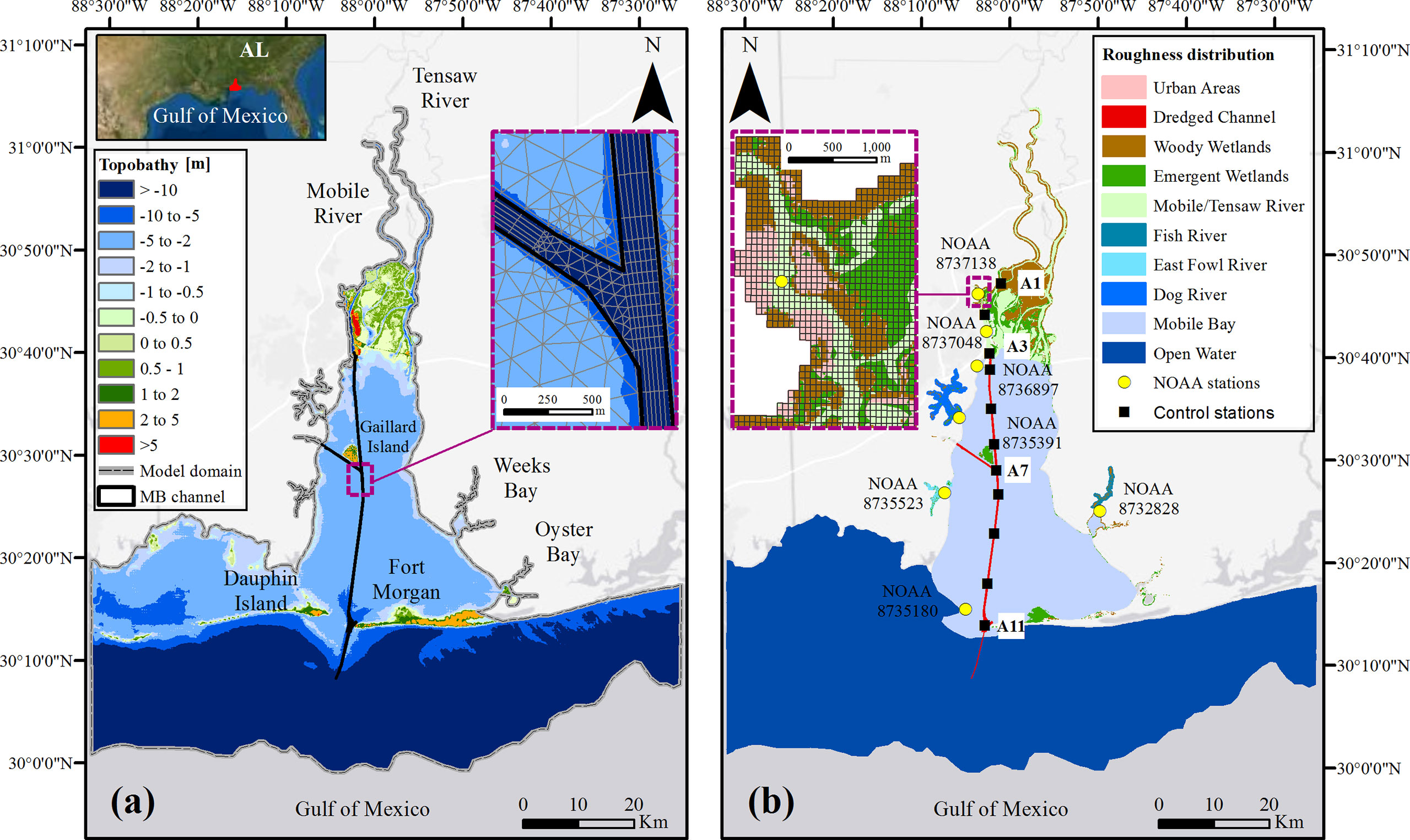
Figure 1 Map of Mobile Bay (MB), AL in the Gulf of Mexico. (A) Topography and bathymetry (topobathy) of MB referenced with respect to the North American Vertical Datum 1988 (NAVD88). Right box shows a detailed view of the unstructured mesh generated to accurately represent the MB channel. (B) Land cover classes and associated roughness distribution used for model calibration at NOAA stations (yellow circles). Left box shows a fine mesh resolution used to simulate wetland inundation around the navigational channel. Control stations (black squares) are used to compute water level profiles.

Navigation of deep-draft vessels (e.g., Neopanamax) through the MB channel is constrained by limited channel depth and width configurations that only allow for one-way daylight traffic and vessel navigation of reduced cargo capacity (e.g., range of 6k – 8.5k TEU). In that regard, the USACE proposed a harbor deepening and channel dredging design to improve vessel navigation and reduce traffic delays along the channel. The “Signed Record of Decision for Mobile Bay Harbor” and related appendices contain detailed information of economic, engineering, environmental, and social studies conducted as part of the project (USACE, 2019). The project was approved in September 2019 and consists of six construction phases to be finalized in March 2025 (USACE GRR, 2019). Specifically, phase 1 and 3 are currently under construction and expected to be completed in September 2022 (USACE DIS, 2022). In summary, the authorized navigation improvements in the channel include: (i) deepen the existing Bar, Bay and River Channels to a total project depth (w.r.t. mean lower low water datum) of 56 ft (17.07 m), 54 ft (16.46 m), and 54 ft (16.46 m), respectively, (ii) incorporate minor bend easings in the Bar Channel approach to the Bay Channel, (iii) widen the Bay Channel from 400 ft (121.92 m) to 500 ft (152.40 m), and (iv) expand the Choctaw Pass Turning Basin 250 ft (76.20 m) to the south.

2.2 Data and Hydrodynamic Model

We use publicly available data to setup a hydrodynamic model of MB and generate a set of scenarios with a combination of forcing conditions, SLR projections by the end of the 21^st century, and dredging protocols established by the U.S. Army Corps of Engineers (USACE, 2019). Hourly time series of RF and coastal WL are retrieved from the U.S. Geological Survey’s (USGS) website mapper (https://maps.waterdata.usgs.gov/mapper/index.html) and the National Oceanic and Atmospheric Administration’s (NOAA) Tide and Currents portal (https://tidesandcurrents.noaa.gov/). Local rainfall, wind, and atmospheric (sea level) pressure are derived from the ERA5 reanalysis dataset (https://www.ecmwf.int/en/forecasts/datasets/reanalysis-datasets/era5) and consists of gridded hourly data with a spatial resolution of 30 km. SLR projections for RCP 4.5 and 8.5 are those estimated by Kopp et al. (2017) using DeConto and Pollard (2016) Antarctic ice-sheet’s projections (DP16’s AIS) and include 5th, 50th, and 95th percentiles. Flood stage thresholds at NOOA’s tide gauges (e.g., minor, moderate, and major flood) are obtained from the National Weather Service (https://water.weather.gov/ahps/) and referenced with respect to the North American Vertical Datum 1988 (NAVD88).

Topography and bathymetric (topobathy) data are obtained from the “Continuously Updated Digital Elevation Model (2019 CUDEM)” of the NOAA's Data Access Viewer (https://coast.noaa.gov/). The topobathy data are vertically referenced with respect to NAVD88 and have a spatial resolution of 3 m. Topobathy data utilized for DEM generation are obtained from a variety of sources, including (but not limited to) the NOAA Office of Coast Survey, NOAA National Geodetic Survey, NOAA Office for Coastal Management, USGS, and the USACE. Georeferenced navigation charts of the Alabama River are updated in a yearly basis and contain satellite imagery, bridge clearance tables, elevated and submerged crossings (USACE, 2021). Manning's roughness distribution in MB are initially derived from the 2019 National Land Cover Database (NLCD) (https://www.mrlc.gov/data) and then refined to account for the navigational channel and river beds in the MB model (Figure 1B). The NLCD map has a 30 m spatial resolution and 16 land cover classes. For simplicity, these developed (urban) classes are re-grouped into a more general classification to avoid unnecessary specificity required in model calibration (see section 2.3.2 for details). The MB model is developed using the 2021 Delft3D-FM suite package in 2D (depth-averaged) mode (Roelvink and Van Banning, 1995). Delft3D-FM solves the continuity and momentum equations using an unstructured finite volume grid under the assumption that vertical length scales are significantly smaller than the horizontal ones (Lesser et al., 2004). Several studies have relied on the suite package to solve complex riverine and estuarine hydrodynamics at local and regional scale with satisfactory results (Kumbier et al., 2018; Bevacqua et al., 2019; Muis et al., 2019). We setup and calibrate the model considering current bathymetry along the MB channel and after additional dredging, i.e., widening and deepening of the channel, for navigation improvement.

2.2.1 Model Configuration

We generate an unstructured mesh consisting of triangular cells over the Gulf of Mexico and the Bay, curvilinear cells in the Mobile River, Tensaw River and MB channel, and rectangular cells over adjacent wetlands (Figure 1). The unstructured mesh can represent complex geomorphological features (e.g., sinuous and/or braided river waterways) with greater detail than traditionally structured grids and allows for local refinement over wetlands, urbanized areas, and harbors (Deltares, 2021). In addition, it aids in simulation efficiency, and is computationally efficient for accurate representation of simulated states (Kumar et al., 2009; Wang et al., 2018). The MB model uses a varying mesh cell-size of 10 m, 60 m, and 1500 m in the navigational channel, wetlands, and Gulf of Mexico, respectively. The model is forced by six upstream RF boundary conditions (BCs) obtained from the U.S. Geological survey (USGS) and NOAA repository including Mobile River (USGS station ID: 02470629), Tensaw River (02471019), Chickasaw Creek (02471001), Fowl River (02471078), Fish River (02378500) and Magnolia River (0237830). For simplicity, we assign time series of hourly water level (WL) from Dauphin Island (NOAA station ID: 8735180) to the ocean boundary as a proxy of coastal WL variability. Moreover, we consider local wind, sea level pressure, and rainfall as additional forcing data for simulating non-extreme and hurricane events.

Vertical bias (elevation errors) of available topographic and bathymetric (topobathy) data (see Section 2.2) is corrected in wetland areas prior to interpolation over the unstructured mesh. For this, we used a ‘DEM-correction’ tool that adjusts surface elevation in coastal wetlands based on ‘emergent herbaceous’ wetland coverage of the 2019 NLCD. The tool corrects lidar-derived DEMs through linear elevation adjustment and site-specific parameters (Alizad et al., 2018) and has been used to improve topobathy data of other hydrodynamic models in the Gulf and Atlantic Coasts of the U.S. (Muñoz et al., 2019; Muñoz et al., 2020; Jafarzadegan et al., 2021b). To account for dredging protocols in the model simulations, we modify the bathymetry of the MB channel (e.g., from control station A2 to A11, Figure 1B) according to the approved dimensions for (i) channel widening, (ii) channel deepening, (iii) entrance expansion, and (iv) minor bend easings (USACE, 2019).

2.2.2 Marsh Migration Tool

In addition to the vertical bias correction, we estimate future wetland spatial distribution and elevation using the “marsh migration tool” from the NOAA’s Sea Level Rise Viewer (https://coast.noaa.gov/slr/). The tool allows for SLR scenario generation and analysis of the associated impacts on local marshes. Specifically, the tool helps delineate wetland regions resulting from five local SLR projections either by individual scenarios (e.g., intermediate low, intermediate, intermediate high, and high) or years (2000, 2020, 2040, 2060, and 2100). We estimate wetland spatial distribution using available data of Dauphin Island as this is a representative area of local conditions in MB (e.g., tidal regime, land subsidence, and wetland types). Regarding wetland elevation, we set an average accretion rate of 6 mm/year in the marsh migration tool based on pertinent literature that includes (i) analyses of marsh and soil core samples extracted next to the MB channel (Runion et al., 2021), and (ii) historical inorganic sedimentation and organic matter accumulation records in several wetland types within the Mobile River, Tensaw River, Mon Louis, and Oyster Bay (Smith et al., 2013). Also, we calculate the total accumulated sediment over future wetland regions (e.g., using the tool, accretion rate, and period 2019 – 2100) and then modify topobathy data of MB. These data are interpolated over the unstructured mesh to generate a set of hydrodynamic models representing both wetland migration and elevation adjustment for SLR projections under RCP 4.5 and 8.5. Furthermore, we use the spatial distribution of future wetland regions including open water to assign roughness values, accordingly. It is worth mentioning that the marsh migration tool subtracts the accretion amount from the total predicted SLR for any given scenario, and it does not account for the effects of erosion and urbanization over time.

2.2.3 Model Calibration

To calibrate the MB model, we regroup and refine the original 2019 NLCD classes into several categories as follows: open water (Gulf of Mexico), estuarine water (Mobile Bay), riverine water (Mobile, Tensaw, Fish, East Fowl, and Dog rivers), navigational (dredged) channel, emergent and woody wetlands, and urban areas (Figure 1B). Then, we set a range of possible Manning’s (n) roughness values (e.g., lower and upper limits) for each of these categories based on recommended values from pertinent literature and hydrodynamic studies (Chow, 1959; Arcement and Schneider, 1989; Liu et al., 2018). The n-values are generated with the Latin Hypercube Sampling (LHS) technique and then calibrated using ensemble model simulations as suggested in recent coastal flood hazard assessments (Jafarzadegan et al., 2021a; Muñoz et al., 2022). Specifically, we generate 200 ensemble members and assign to them a unique combination of n-values (Table 1).

TABLE 1

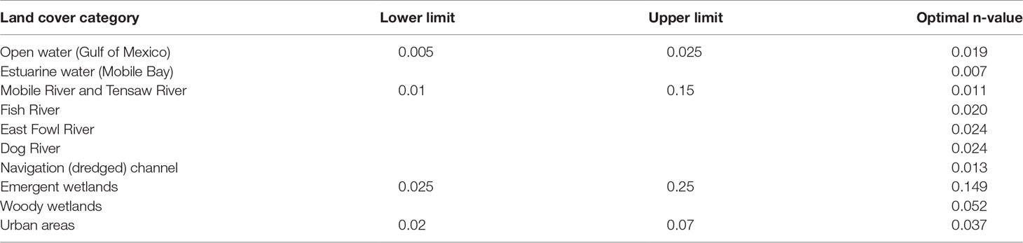
Table 1 Range of Manning’s roughness values used for calibration of the Mobile Bay model.

The goal of model calibration is to identify an optimal combination of n-values (or alternatively the best ensemble member) that minimizes the root-mean square error (RMSE) between observed and simulated WLs, while also producing the highest Nash-Sutcliffe efficiency (NSE) (Nash and Sutcliffe, 1970) and Kling-Gupta efficiency (KGE) coefficients (Gupta et al., 2009). NSE ranges from 0 to 1 whereas KGE can take values between -∞ and 1. For these evaluation metrics, an efficiency of 1 indicates a perfect match between observations and model simulations. Also, RMSEs below 0.20 m are desirable for simulating extreme events on the U.S. Gulf-Atlantic Coasts (HSSOFS, 2015). To ensure the MB model can represent extreme WLs, we simulate Hurricane Ida that hit the Gulf of Mexico on Aug/Sep 2021. Ida was the costliest disaster in 2021 exceeding $60 billion and caused extreme storm-surge, strong sustained winds, and torrential rainfall over the coasts of Louisiana, Mississippi, and Alabama (NCEI, 2021). We set a warm-up period from Aug/1 to Aug/22 to ensure a correct propagation of tides and river-induced WL over the model domain. WL variability resulting from the last time step is then used as a ‘hot start’ file to begin with model calibration of the following days up to Sep/6 (see Section 3.2).

2.3 Statistical Framework

2.3.1 Sampling Strategy

We analyze the statistical dependence between flood drivers in MB (e.g., RF and coastal WL) using joint probability density functions. Among the available gauge and tide stations in the MB watershed, we select RF records from Tombigbee River station (USGS ID: 02469761) located upstream of the Mobile River and Tensaw River, and WL records from Dauphin Island station (Figure 1). These stations have relatively long records starting in 1960 and 1981, respectively, and therefore allow for estimating return periods at lower frequencies (e.g., 50-year). The procedure for sampling flood-driver pairs consists of peak-over-threshold, with twice the length of the available records, i.e., 80 total compound samples from two-sided sampling and/or 40 samples each side. Since compound effects of flood drivers do not necessarily coincide in time, we consider a maximum lag-time of 7 days between sampled events as suggested in compound flood (CF) studies conducted at local, regional, and global scales (Klerk et al., 2015; Moftakhari et al., 2017; Ward et al., 2018; Nasr et al., 2021).

2.3.2 Bivariate Statistical Analysis

To characterize the joint probability of RF and WL, we used a copula-based approach in which the correlation structure of flood drivers is disentangled from its marginals (Nelsen, 2007; Joe, 2014). Hence, the advantage of copulas over traditional multivariate approaches is that marginal distributions are not constrained by the same probability family as well as the same parameters ruling both marginals and the multivariate dependence (Salvadori et al., 2007; AghaKouchak et al., 2012; Madadgar and Moradkhani, 2013). According to the Sklar’s theorem (Sklar, 1959), there exists a copula function C(C_RF,WL: [0,1] × [0,1] → [0,1]) of the pair (RF,WL), with marginal cumulative distribution functions F_RF and F_WL, for all (RF,WL) ∈ R², as shown in Equation (1):

$\begin{array}{ll}{F}_{RF,WL}\left(RF,WL\right)=C_{RF,WL}\left[F_{RF}\left(RF\right),F_{WL}\left(WL\right)\right]& (1)\end{array}$

For convenience, we conduct a bivariate statistical analysis using the Multi-hazard Scenario Analysis Toolbox (MhAST) developed by Sadegh et al., (2017, 2018 ). This tool has been used in similar studies with satisfactory results (Didier et al., 2019; Moftakhari et al., 2019; Muñoz et al., 2020). MhAST fits univariate distribution functions to the marginals and suitable copula-based functions to flood-driver pairs with their underlying uncertainties. The toolbox considers 17 different continuous marginal distributions and estimates their parameters using a maximum likelihood algorithm. The best distribution that optimally fits the available data is determined using the Bayesian information criterion. Furthermore, MhAST considers 26 copula families and identifies the best one that describes the correlation structure based on the Akaike information criterion, Bayesian information criterion, and maximum likelihood. Hereinafter, we refer to the joint probability of RF and WL as ‘AND scenario’ in which both flood drivers exceed a certain threshold (Figure 2). Based on the correlation structure of the drivers, we focus on bivariate occurrences that fall along the 50-year iso-return period curve. Specifically, we identify the most likely flood-driver pair for the AND scenario and then estimate both upstream and downstream BCs for hydrodynamic simulations (see Section 3.1).

FIGURE 2

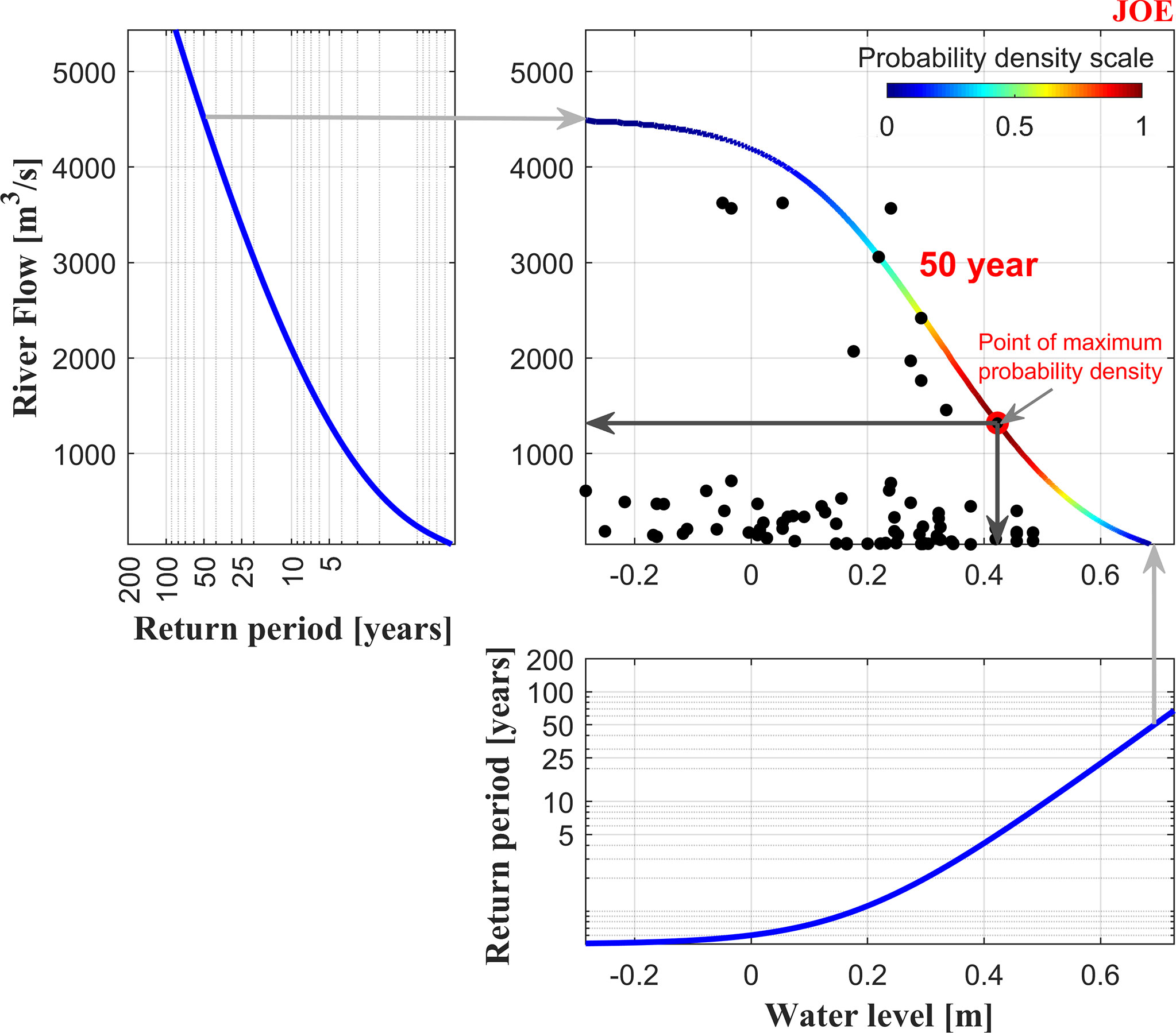
Figure 2 Bivariate statistical analysis of flood drivers in Mobile Bay, AL. Marginal probability density of river flow (RF) and coastal water level (WL) with 50-year return level pairs around the corresponding iso-return period curve. Black scattered dots show bivariate occurrences of the flood drivers whereas red dot represents the point of maximum probability density based on the correlation structure of RF and WL.

To generate the compound flood scenarios, we consider a river gauge station located at the head of both Mobile River and Tensaw River (USGS ID: 02469761) as those two contribute with ~95% of the freshwater inflow to MB (Schroeder, 1978). We further calculate that those rivers contribute with 48% and 47% of the annual freshwater inflow to MB, respectively, and therefore we neglect RFs from Chickasaw Creek, Fowl River, Fish River, and Magnolia River. Nevertheless, their corresponding RFs are considered in the model calibration process for Hurricane Ida. Also, we only consider two main rivers (e.g., Mobile and Tensaw) to simulate RF resulting from the bivariate copula analysis and split the discharge based on the corresponding percentages, which in fact are almost identical, i.e., about half of the estimated RF is assigned to each river. The statistical methodology presented in this study is similar to recent works that often neglect the contribution or river tributaries for the sake of simplicity [e.g., Moftakhari et al. (2017); Bevacqua et al. (2019), and Jafarzadegan et al. (2022)].

3 Results and Discussion

3.1 Statistical Scenarios

The copula-based approach reveals that RF and WL are negatively correlated in terms of Kendall’s rank (τ) and Spearman’s rank (ρ) correlation coefficients and their associated p-values (Table 2). We found that these coefficients are statistically significant at 5% level (p-value ≤ 0.05) and the most suitable joint probability function that fit the data is the Joe copula family.

TABLE 2

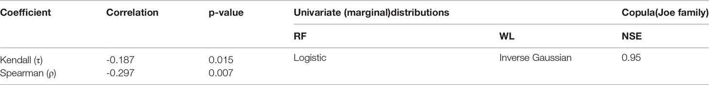
Table 2 Correlation structure of flood drivers in Mobile Bay, AL.

The bivariate statistical analysis in addition to available information from USGS and NOAA stations (e.g., gauge datum and vertical datum of tides) help define a set of BCs for hydrodynamic simulations. The BCs represent a baseline or M-M scenario consisting of mean RF (50^th percentile) and mean WL (mean sea level), L-L scenario derived from low RF (5^th percentile) and low WL (mean lower low water), H-H scenario consisting of high RF (95^th percentile) and high WL (mean higher high water), and CF (AND) scenario characterizing a 50-year return period event. Combinations of those BCs, topobathy data with current conditions and dredging protocols (USACE, 2019), and SLR projections under RCPs 4.5 and 8.5 (Kopp et al., 2017) result in a total of 44 statistical scenarios (Table 3). These scenarios are run for a single spring-neap tidal cycle to account for high and low tides (e.g., 15-day simulation period). For simplicity, we exclude scenarios that combine low and high flood drivers and low-low flood drivers plus SLR since the WLs resulting from these scenarios will likely be encompassed by the scenarios already proposed in Table 3.

TABLE 3

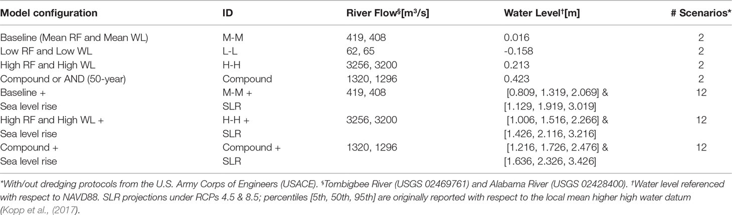
Table 3 Statistical scenarios for hydrodynamic simulation derived from statistical analyses in Mobile Bay, AL.

3.2 Model Simulations

We calibrate the model twice using topobathy representing current conditions and channel modification due to dredging protocols. Nevertheless, we did not find considerable differences between Manning’s n-values in the MB channel. Specifically, we observed only small differences in the third decimal of the calibrated values. Regarding the evaluation metrics of simulated versus observed WLs (Figure 3), RMSE is below 0.11 m whereas NSE and KGE are above 0.85 and 0.80, respectively. These results indicate that the MB model is satisfactorily calibrated for simulating extreme events such as Hurricane Ida (HSSOFS, 2015), and can also accurately represent non-extreme WLs. Note that Mobile State Docks (Figure 3D) and Coast Guard Mobile (Figure 3F) achieve the highest RMSE and lowest NSE and KGE. These results may reveal inaccuracies in the topobathy data or suggest that additional mesh-refinement is required around those locations to improve simulations of peak and low WLs. Nevertheless, there is always a trade-off between computational time and mesh resolution (cell-size) for hydrodynamic simulations.

FIGURE 3

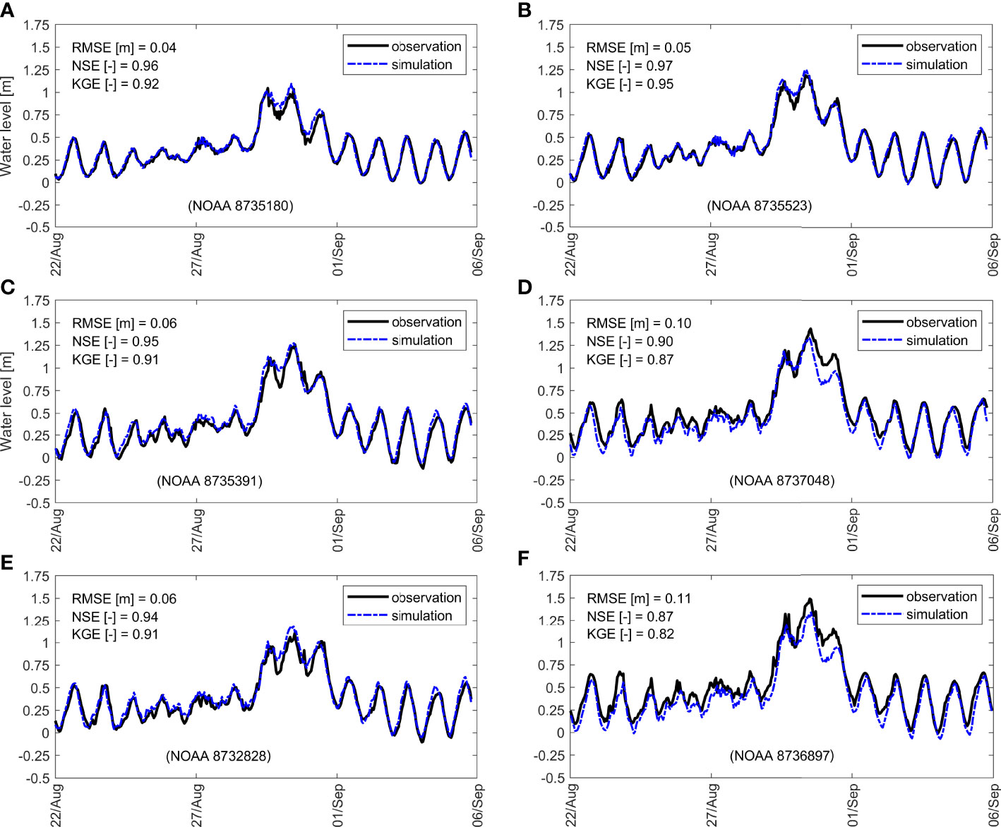
Figure 3 Model calibration of Mobile Bay at tide-gauge (NOAA) stations: (A) Dauphin Island, (B) East Fowl River, (C) Dog River, (D) Mobile State Docks, (E) Weeks Bay, and (F) Coast Guard Mobile. Observed (black solid line) and simulated water levels (blue dashed line) correspond to Hurricane Ida (Aug/Sep 2021). Model performance is evaluated in terms of Root-mean squared error (RMSE), Nash-Sutcliffe efficiency (NSE), and Kling-Gupta efficiency (KGE).

3.3 Compound Effects on Vessel Navigability

3.3.1 Water Surface Elevation, Tidal Range, and Clearance Profiles

We compute profiles over control stations conveniently distributed in the Mobile River (A1 – A3) and the Bay (A3 – A11) [Figures 4 and S1 (Supplementary Material)]. The profiles show mean WSEs (top panel), mean tidal ranges (middle panel), and underkeel clearances (bottom panel) obtained from scenarios with current bathymetry (solid lines), and after deepening and widening of the navigational channel (dashed lines). There is a negligible reduction of WSE for all scenarios after channel dredging and under current mean sea level (Figure 4A). However, note that both H-H scenarios show a progressive increment of WSE between control stations A4 and A1 with respect to the baseline (e.g., values ranging from 0.25 m up to 1 m, respectively). Particularly, there is a considerable increment of WSE (~0.75 m) at Bay Bridge/Cochrane-Africatown Road located between control stations A1 and A2. Nonetheless, Bay Bridge’s bottom elevation is 44 m referenced with respect to NAVD88 (USACE, 2021) and so provides enough vertical clearance for vessels to navigate underneath. Such an increment of WSE at the head of the navigation channel results from high RF in the Mobile River (95^th percentile, Table 3) that also leads to a reduction of tidal range and/or frictional damping of the tide with respect to the baseline. High RF attenuates the incoming tide wave at the most upstream control stations (A3 – A1) where the tidal range decreases below 0.40 m. In contrast, low RF regimes do not attenuate the tide wave, but increase tidal ranges above 0.50 m for the same stations (Figure 4C). Tidal damping due to increased RF has been reported in other rivers around the globe including the Saint Lawrence River (Godin, 1999), Columbia River (Kukulka and Jay, 2003), Yangtze River (Guo et al., 2015), Garonne River (Jalón-Rojas et al., 2018), among others. Moreover, our hydrodynamic results agree well with those from analytical models as they have shown that increasing RFs reduce tidal range due to enhanced tidal friction, delay wave propagation, and progressively attenuate tidal energy distribution among tidal frequencies (Godin, 1985; Jay, 1991; Sassi and Hoitink, 2013; Cai et al., 2014; Guo et al., 2015). Yet, computations of tidal energy, tidal and RF velocities in MB are out of the scope of this study.

FIGURE 4

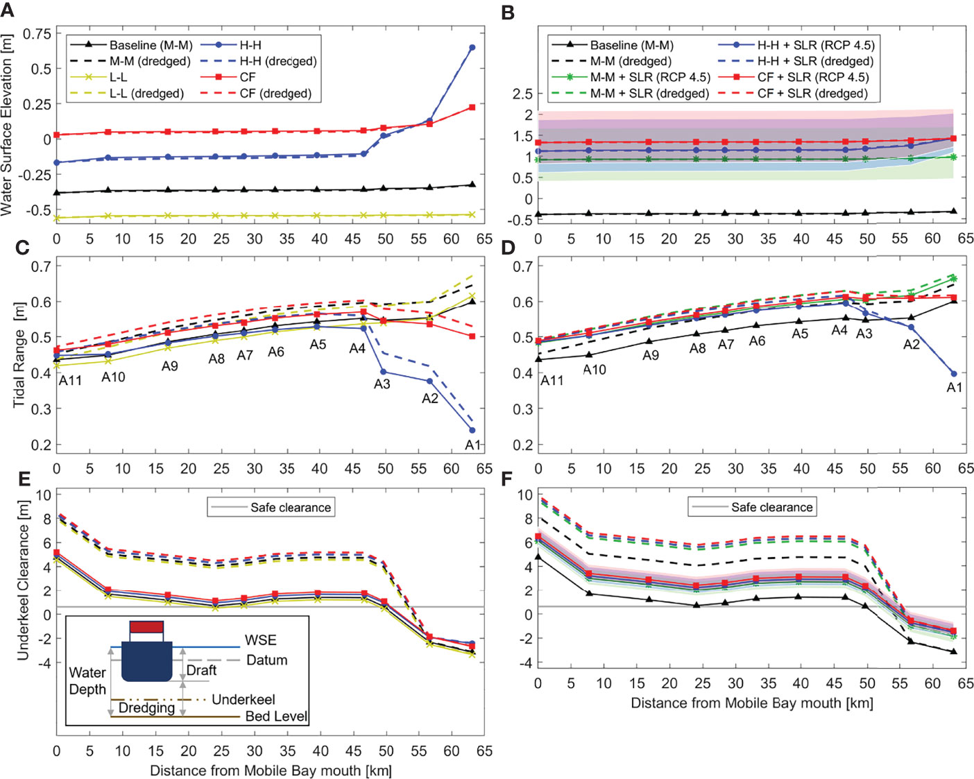
Figure 4 Profiles along control stations (A1 to A11) in the Mobile Bay channel with current bathymetry (solid line) and after channel dredging (dashed line). The scenarios consider mean river flow (RF) and mean sea level (M-M scenario), low RF and mean lower low water (L-L), high RF and mean higher high water (H-H), and Compound flood (50-year return period) under current mean sea level (left panel) and sea level rise projections at Dauphin Island (right panel). Profiles show (A, B) mean water surface elevation (WSE), (C, D) mean tide range, and (E, F) underkeel clearance (U) for safe navigation where the gray horizontal line represents a threshold-value that prevents any potential damages to vessels. Shaded bands indicate WSEs and U-values between 5^th and 95^th percentiles. Left bottom corner shows a schematic of a draft-vessel and the associated clearance. Mobile Harbor is located at control station A3.

On the other hand, our results show that the average tidal range along the dredged channel increases by a factor of ~1.1 for all scenarios with respect to those with current bathymetry. In general, channel dredging increases WD and so reduces the effects of bottom friction leading to an increase of tidal amplitudes. Similarly, other studies around the globe have reported an increase of tidal range associated with channel dredging in riverine-estuarine systems including the Modaomen estuary (Cai et al., 2012), Elb and Ems estuaries (Winterwerp et al., 2013), Rhine-Meuse delta (Vellinga et al., 2014), Loire estuary (Jalón-Rojas et al., 2016), Cape Fear River (Familkhalili and Talke, 2016), Hudson River (Ralston et al., 2019), among others. Next, we compute bottom or ‘underkeel’ clearances (U) in the MB channel, i.e., vertical difference between mean WD and draft vessel (Equation 2), and identify control stations where U is at least 2 ft (0.61 m). This threshold-value prevents any potential damages to vessels (e.g., hulls, rudders, and propellers) due to bottom channel irregularities.

$\begin{array}{ll}U=WD-D=WSE-BL-D& (2)\end{array}$

where WD is calculated in terms of WSE and bed level (BL), and D is the static-draft vessel obtained from technical specifications and/or manual of operations. Negative U-values indicate shallow waters that impede vessel navigation especially in upstream riverine channels. We estimate U-values for each scenario based on the largest vessel registered in Mobile Harbor (e.g., draft-vessel of 47.5 ft (14.48 m) according to the USACE (2019) and then analyze the compound effects of flood drivers and channel dredging on navigation (Figure 4E). The current dimensions of the channel allow vessels to navigate between the MB entrance and Mobile Port (A11 to A3) under each scenario. Yet, vessel navigation is compromised on shallow waters (e.g., 40 ft (12.19 m)) especially over the submerged Bankhead and Wallace Tunnels located upstream control station A3. Nevertheless, the authorized dredging protocols between control stations A11 to A3 help increase U-values up to 4.39 m in average for all scenarios with respect to the threshold value, or alternatively by a factor of 3.33 with respect to the baseline scenario without channel dredging. This in turn allows navigation of deeper-draft vessels well above the safe clearance threshold.

SLR increases WSE along the MB channel and diminishes the effects of channel dredging on WL profiles (Figures 4B and Supplementary Figure 1A). Particularly, WL profiles computed with current bathymetry and dredging protocols show negligible differences and/or almost identical WSEs. Note that we include the baseline scenario in both figures for a better comparison among the scenarios with/out SLR. The CF scenario shows the highest WSE which in turn reduces the vertical clearance of Bay Bridge (44 m) by 1.72 m and 2.31 m under RCP 4.5 and 8.5, respectively. Regarding tidal ranges, SLR diminishes the effects of high RF on tidal damping along the Mobile River (A1 – A3) as compared to the H-H scenario in Figure 4C. This in turn makes the CF scenario the most extreme showing the highest WSEs at any control stations and the surrounding wetlands (see Section 3.4). Furthermore, SLR increases the tidal amplitude of M-M and H-H scenarios and as a result the tidal range along the Bay (A3 – A11) is close to that of the CF scenario under both RCP 4.5 and 8.5 (Figures 4D and Supplementary Figure 1B, respectively). Overall, tidal range in MB increases in landward direction except for the H-H scenario where the nonlinear interactions of SLR, tides, and RF contribute to frictional damping of the tide as observed at control station A1 (e.g., ~0.4 m and 0.55m for RCP 4.5 and 8.5, respectively). The effects of SLR on tidal dynamics are complex as they result from nonlinear interactions among forcing drivers, estuarine morphology, fluid properties, and friction factors. A comprehensive modeling approach of estuarine tidal response to both rising sea levels and RF scenarios showed that tides are either attenuated in short estuaries characterized by low tidal ranges or amplified in prismatic and converging estuary types (Khojasteh et al., 2021a; Khojasteh et al., 2021b). Specifically, our results suggest that SLR will increase tidal range along the navigational channel (e.g., 9.9 cm for M-M scenario and under RCP 4.5 and 8.5, respectively) and agree well with similar studies conducted in the Gulf of Mexico (e.g., an increase up to 10.0 cm under the 2100-high scenario (Passeri et al., 2016)). Yet, tidal response to SLR may vary in space and so experience localized attenuation or amplification with tidal amplitudes not proportional to the changes in mean sea level (Pickering et al., 2012; Lee et al., 2017; Palmer et al., 2019). Lastly, we analyze the compound effects of SLR, flood drivers, and channel dredging on vessel navigation and estimate that U-values increase up to 5.83 m and 6.43 m in average for all scenarios with respect to the threshold value, or alternatively by a factor of 4.20 and 4.60 with respect to the baseline scenario without channel dredging and under RCP 4.5 (Figure 4F) and 8.5 (Supplementary Figure 1C), respectively.

3.3.2 Navigation Charts

To further analyze the compound effects on navigable waters, we generate navigation charts with contour lines of mean WSE at selected control stations (Figure 5). We use the Latin Hypercube Sampling technique (Helton and Davis, 2003) to generate 200 combinations of RF and WL forcing and then conduct model simulations in parallel by leveraging a high-performance computing system. The upstream and downstream BCs represent realistic statistical scenarios for MB (Table 3) and include maximum and minimum observed tides in Dauphin Island station from NOAA’s Tide and Currents web portal. We fill gaps between contour lines and create a smooth navigation chart using the ‘scattered Interpolant’ function with a nearest-neighbor interpolator available in MATLAB. Results from this analysis show a gentle (negative) slope for all black contour lines indicating that mean WSE is more sensitive to changes of coastal WL than RF for M-M, CF, and H-H scenarios. The latter helps delineate safe and hazard zones for MB associated with multiple combinations of BCs. Specifically, the charts show three hazard zones including a vessel damage area [U< 0.61 m, Equation (2)], minor flooding (WSE > MHHW + 0.518 m), moderate flooding (WSE > MHHW + 0.914 m), and major flooding (WSE > MHHW + 1.829). Minor, moderate, and major flooding thresholds are derived from pre-established flood categories of the NOAA’s National Weather Service. In addition, we identify a safe clearance zone where WSEs are suitable for navigation and do not represent a flood hazard for the surrounding urban and natural (wetland) areas.

FIGURE 5

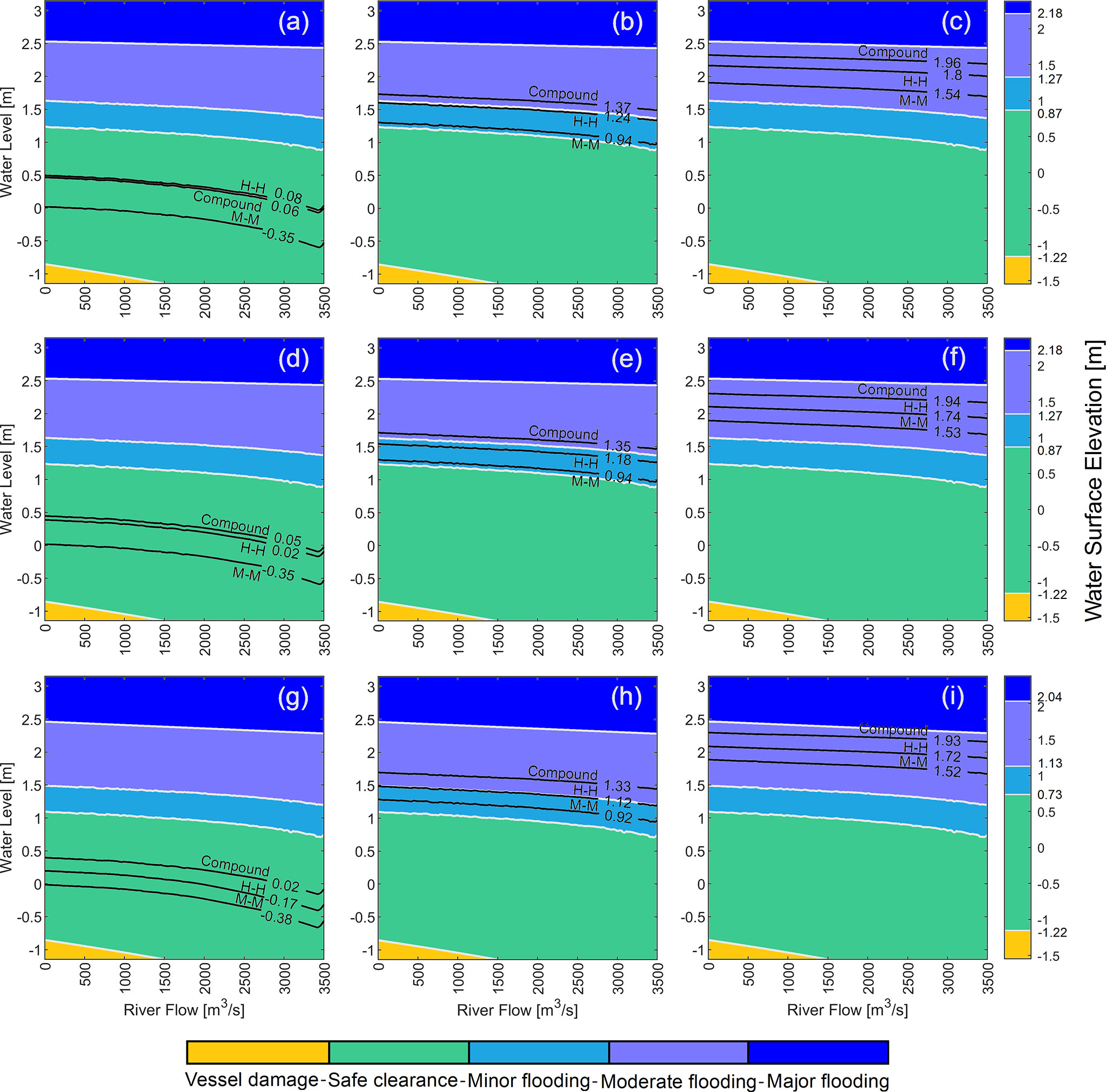
Figure 5 Mean water surface elevation (WSE) as a function of upstream and downstream forcing conditions and dredging protocols. Black contour lines represent WSE obtained from M-M (baseline), H-H, and CF scenarios at selected control stations in the Mobile Bay channel: A2 (A–C), A3 (D–F), and A11 (G–I). Gray lines represent threshold values for safe navigation and hazard zones (color bar). Left, middle, and right panels show WSE simulated with current mean sea level, and sea level rise projections under RCP 4.5 (50^th percentile), and RCP 8.5 (50^th percentile), respectively.

In general, the CF scenario leads to the highest WSEs at the selected control stations for both current mean sea level (Figure 5, left panel) and SLR projections (middle and right panels) even though RF is ~2.5 times smaller than that of H-H scenario. This suggests that coastal WL is the dominant flood driver in MB, and also explains the gentle slope inferred from the contour lines in the navigation charts. Moreover, the relative influence of RF on WSE is evident at control stations in the Mobile River (Figures 5A, D) where the contour lines of H-H and CF scenarios are almost identical. The effects of SLR on WSE are also evident in the navigation charts since changes in mean sea level shift the contour lines in upward direction, and as a result both H-H and CF scenarios trigger minor or moderate flooding (Figure 5, middle and right panels). It is worth noting that wetland areas can act as natural buffers dissipating storm surge at a rate of 1.7 to 25 cm/km (Leonardi et al., 2018) and minimize flood risks and damages associated with coastal storms and/or SLR (Rezaie et al., 2020; Sun and Carson, 2020). In that regard, existing wetland areas next to the Mobile River channel (~34.38 km²) might have altered the propagation of extreme WL and RF and reduced WSEs in the MB channel (Figure 5, left panel). Likewise, wetland losses due to SLR under RCP 4.5 (~88%) and RCP 8.5 (~91%) might have reduced the storm surge attenuation capacity of the system in spite of a sediment accretion rate of 6 mm/year in MB. The latter in addition to extreme WLs associated with the SLR projections progressively increase WSEs (Figure 5, middle and right panels). From a decision-make point of view, local stake holders and policy makers can benefit from the proposed charts as they allow for an integrated navigation and flood hazard assessment given a combination of BCs, dredging protocols, and SLR projections. Next to the proposed CF scenario, the navigation charts can be modified or updated to account for events with larger return periods (> 50-year) and other RCPs (e.g., 2.6 and 6) projected by mid- or at the end of the 21^st century. Likewise, similar charts can be generated at any locations (or control stations) in the study area based on simulated WSE and forcing conditions.

3.4 Compound Effects on Wetland Inundation Dynamics

We construct PDFs of wetland inundation (Figure 6) using flood composites around the Mobile River and the underlying future wetland distribution (see Section 2.2.2). The composites of each scenario represent maximum WSEs simulated for a 15-day period (spring-neap tidal cycle) with/without bathymetric (channel) modification. We consider WSE data with a temporal resolution of 15 min and pixel-resolution of 60 m x 60 m to ensure a uniform spatiotemporal sampling and interpolation over wetland areas (Figure 1B). The PDFs are constructed using a kernel density function to circumvent any erroneous inferences/assumptions of data distribution. Results from this analysis suggest that flood drivers and channel dredging do not alter wetland inundation dynamics, specifically for scenarios with low to moderate RF regimes (e.g., L-L, M-M, and CF) as their PDFs are almost identical (Figure 6A, solid vs. dashed lines). Maximum WSEs of L-L, M-M, and CF scenarios are centered around 0.45 m, 0.45 m, and 0.6 m, respectively, and do not represent a flood hazard for the surrounding areas. In contrast, the PDFs of H-H scenario are centered around 0.75 m and 0.95 m suggesting that channel dredging can reduce minor riverine-induced flooding over adjacent wetlands. This in turn may influence fresh and saline water dynamics, hinder sediment transport and deposition, and limit nutrient availability necessary for wetlands to grow (Allison and Meselhe, 2010; Kirwan et al., 2010; Alizad et al., 2016). In general, dredging protocols enhance the hydraulic conveyance capacity of riverine systems (Ralston et al., 2019; Saad and Habib, 2021) and the latter is more evident in MB for scenarios with high RF regimes (95^th percentile, Table 3). Changes in mean sea level due to SLR diminish any effects of channel dredging on wetland inundation dynamics and shift the PDFs beyond pre-established thresholds into moderate (Figure 6B) and major flooding zones (Figure 6C). Also, note that those PDFs resemble a multimodal distribution which is likely attributed to maximum WSEs in lower, intermediate, and upper wetland zones that are more and less exposed to SLR and flood drivers.

FIGURE 6

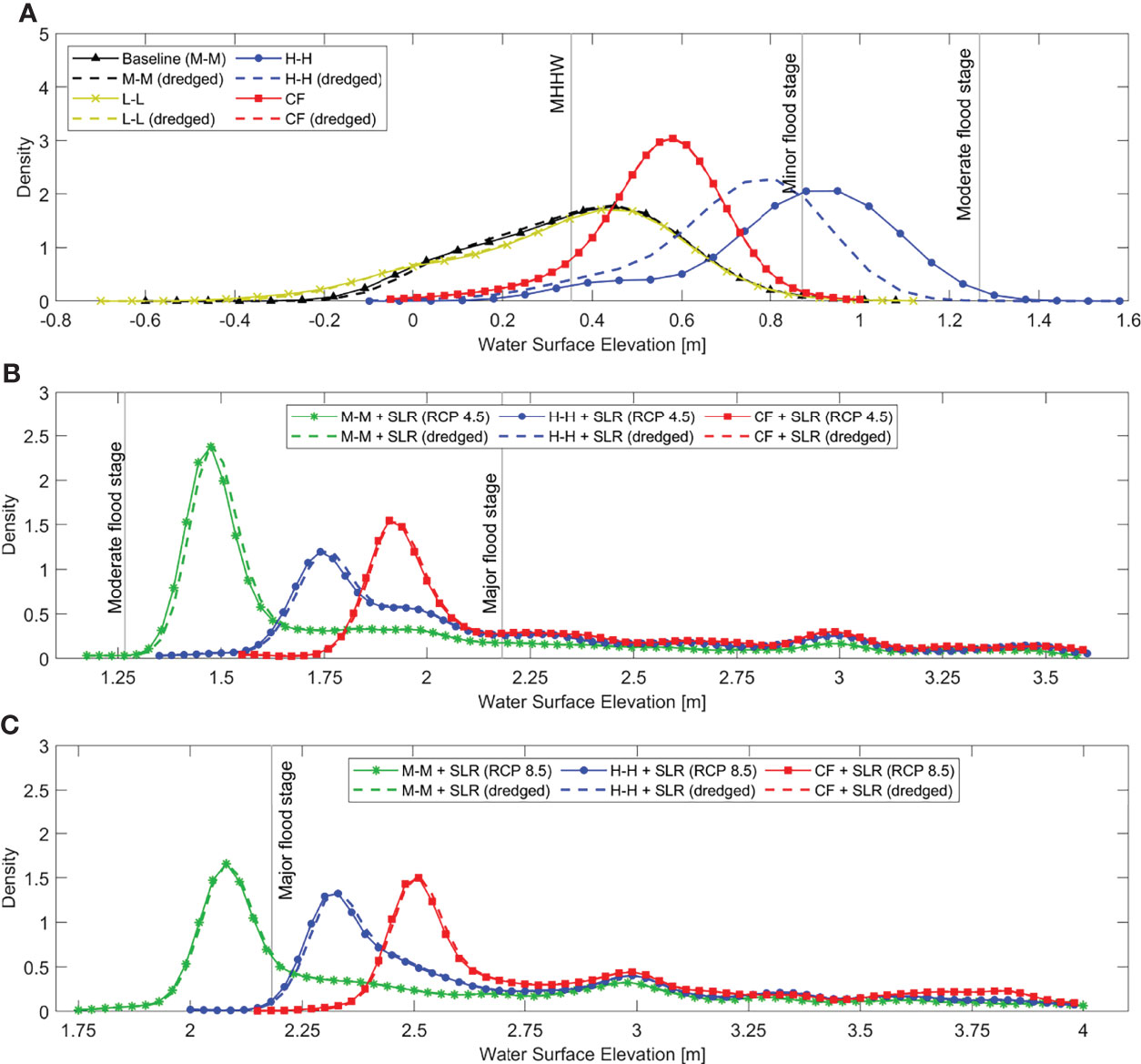
Figure 6 Probability density functions (PDFs) of maximum water surface elevation (WSE) within wetland areas near the Mobile River, AL. The PDFs are constructed based on flood composites simulated with current bathymetry (solid line) and after channel dredging (dashed line). The scenarios consider water level regimes with (A) current mean sea level, and sea level rise projections under (B) RCP 4.5 (50^th percentile), and (C) RCP 8.5 (50^th percentile). Mean higher high water and flood stage thresholds are referenced with respect to NAVD88 and correspond to those of Mobile State Docks tide-gauge (NOAA station ID: 8737048).

Next, we analyze wetland inundation patterns associated with (i) SLR projections (Figure 7) and (ii) channel dredging (Supplementary Figure 2). For the first analysis, we compute maximum WSEs for each scenario under RCP 4.5 and 8.5 and then calculate residuals with respect to the M-M scenario. In that sense, we can meaningfully compare flood composites with respect to each other and against the baseline scenario. We identify non-inundated areas next to the Mobile River channel (A2 – A3) where residuals are practically negligible regardless of the scenarios with flood drivers and SLR projections (e.g., dark blue color). These areas comprise a number of cargo terminals as well as urban and industrial areas that are hardly exposed to flooding due to high terrain elevations (≥ 5 m, NAVD88 datum). Wetland areas located in-between bays, ponds, and tidal channels are exposed to extreme WLs and thereby periodically flooded. Nevertheless, we identify a common inundation pattern characterized by a plain (average) residual in the background and a number of ‘hot spots’ in which the residuals are higher. For example, M-M scenarios under RCP 4.5 and 8.5 show a residual background and hot spots of ~0.75 m – ~1.25 m (Figure 7A) and ~1.5 m – ~2 m (Figure 7B), respectively. Likewise, H-H scenarios show a residual background and hot spots of ~1 m – ~1.5 m (Figure 7C) and ~1.75 m – ~2.25 m (Figure 7D). Yet, the highest residuals are seen in CF scenarios under both SLR projections. Residual background and hot spots for RCP 4.5 and 8.5 are ~1.25 m – ~1.75 (Figure 7E) and ~2 m – ~2.5 m (Figure 7F), respectively. Note that the combination of flood drivers, channel dredging, and SLR leads to a non-linear increase of WLs, which in turn helps explain the complex patterns observed in tidal channels and interior bays and ponds. For the second analysis, we set scenarios generated with current bathymetry as ‘reference’ flood composites and then compute residuals of maximum WSE after channel dredging. L-L and M-M scenarios show positive residuals (~0.10 m) indicating a slight increase of WLs in small tidal channels and interior ponds (Supplementary Figures 2A, B). Yet, residuals over adjacent wetlands are negligible confirming that channel dredging and scenarios with low to moderate flood drivers do not alter wetland inundation patterns. Likewise, residuals under the CF scenario are negligible as a result of extreme WLs that elevate WSE in the system and diminish the effects of RF on tidal damping (Supplementary Figure 2D). In contrast, the largest negative residuals (~0.40 m) result from the H-H scenario suggesting that channel dredging increases Mobile River’s hydraulic conveyance capacity and reduce WLs in the surrounding wetlands (Supplementary Figure 2C).

FIGURE 7

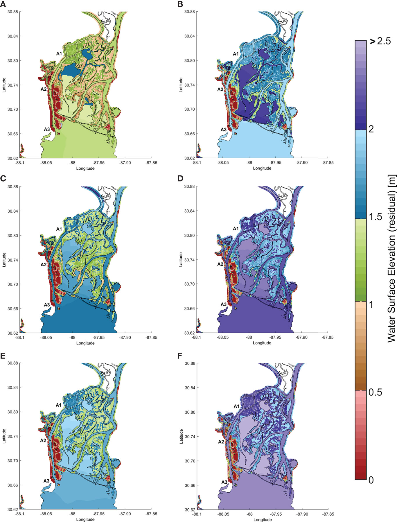
Figure 7 Residuals of maximum water surface elevation (WSE) between the baseline scenario (M-M) and those with sea level rise (SLR) projections: RCP 4.5 (left panel) and 8.5 (right panel). Residuals are computed for (A, B) M-M + SLR, (C, D) H-H + SLR, and (E, F) CF +SLR scenarios. Black polygon delineates the current tidal channel morphology. A1 to A3 are control stations located in the Mobile River channel.

Coastal wetlands in MB are vulnerable to rising waters already observed in Dauphin Island (e.g., 4.25 mm/yr, NOAA ID: 8735180). Our results suggest that SLR will affect the dynamics between tides and freshwater inflow and permanently inundate wetland regions under RCP 4.5 and 8.5 (e.g., above moderate to major flood thresholds, respectively). Marshes can cope with SLR and adapt to changes in sediment supply by migrating to upland areas (Alizad et al., 2016; Kirwan et al., 2016; Schieder et al., 2018), however the marsh migration tool (used here as a proxy of future wetland distribution) predicts considerable wetland losses next to the MB channel under the proposed SLR scenarios (https://coast.noaa.gov/slr/). Although the tool accounts for a sediment accretion rate of 6 mm/year based on field studies (Smith et al., 2013; Runion et al., 2021), it also neglects the effects of erosion and urbanization over time. We argue our ‘hybrid’ physics-informed and statistical modeling approach can be improved for future studies by integrating ecological and morphodynamic feedbacks, and thereby providing a comprehensive assessment of estuarine dynamics to SLR and wetland dynamics (Khojasteh et al., 2021b; Kumbier et al., 2022).

4 Conclusions

Engineering projects are often designed to handle isolated physical hazards. Ignoring compound hazards and their effects can compromise the feasibility and life-cycle of these projects. In this study, we analyze the compound effects of SLR, flood drivers, and channel dredging on vessel navigation and wetland inundation dynamics in Mobile Bay, AL. We hypothesize that dredging protocols will have influence vessel navigability depending on the flood drivers (e.g. fluvial, coastal, and compound) and morphology of estuarine and coastal systems. Also, we expect that flood regimes in addition to SLR will affect wetland dynamics and alter inundation patterns with negligible influence of channel dredging when compared to any baseline conditions (e.g., mean flood regime and current channel bathymetry). To test these hypotheses, we first develop two 2D hydrodynamic models with current and modified bathymetric data that reflect pre- and post-dredging conditions, respectively. The models are rigorously calibrated to infer suitable roughness coefficients that capture WL variability of both non-extreme events and an extreme event in form of hurricane Ida that hit the Gulf Coast of the U.S. on Aug/Sep 2021. We then conduct statistical analyses and derive a set of scenarios representing a range of WL and RF forcing conditions including low, mean, and high regimes. In addition, we consider SLR projections by the end of the century under RCP 4.5 and 8.5. Since the forcing drivers are statistically dependent (p-value ≤ 0.05), we conduct a bivariate copula-based analysis to derive a compound flood scenario representing a 50-year return period. To account for SLR impacts on wetland spatial distribution and elevation, we leveraged the “marsh migration tool” from the NOAA’s Sea Level Rise Viewer. The tool helps delineate wetland regions resulting from local SLR projections and a set of average accretion rates based on local marsh conditions. We calculate the total accumulated sediment over future wetland regions for each SLR projection, and then modify topobathy data of MB and spatial Manning’s roughness values accordingly. Lastly, we run hydrodynamic simulations based on the statistical scenarios and generate (i) longitudinal profiles along the channel, (ii) navigation charts for safe navigation and flood hazard assessment, (iii) PDFs of wetland inundation, and (iv) flood inundation patterns over the channel and adjacent wetland areas.

Results show that channel dredging slightly reduces WSE in all scenarios. and increases tidal range by a factor of 1.1 due to a reduction of frictional resistance associated with channel deepening. Yet, SLR elevates WSE along the channel and increases underkeel clearances by a factor of 4.2 and 4.6 under RCP 4.5 and 8.5, respectively. Although rising waters ensure an optimal navigation preventing any physical damages to vessels (e.g., hulls, rudders, and propellers), they also shift WSE into flood hazard zones (WSE > 0.87 m) triggering minor to major flooding in the surrounding urban and wetland areas. PDFs of wetland inundation indicate that channel dredging can reduce minor riverine-induced flooding over these coastal ecosystems. Moreover, channel dredging enhances the hydraulic conveyance capacity of riverine systems and the latter is more evident for scenarios with high RF regimes. Nonetheless, SLR diminishes any effects of channel dredging on wetland inundation dynamics and shift the PDFs beyond pre-established thresholds for moderate and major flooding. Although wetland inundation patterns are complex to interpret, we identify a common pattern characterized by a plain (average) WSE residual in the background and a number of ‘hot spots’ in which those residuals are higher. These complex patterns are attributed to nonlinear interactions among flood drivers, channel dredging, and SLR. Based on these results, we recommend integrated analyses in other ports and harbors of the world that account for those compound effects on vessel navigation and wetland inundation. Particularly, the connections among compound flooding, climate change, and current engineering practices for harbor maintenance (e.g., channel dredging) can provide insights into environmental-friendly solutions for increasing cargo transportation. All authors contributed to the article and approved the submitted version.

Data Availability Statement

The original contributions presented in the study are included in the article/Supplementary Material. Further inquiries can be directed to the corresponding author.

Author Contributions

DM and HMof conceptualized the study. DM wrote the initial manuscript. HMof supervised the work and edited the manuscript. MK, and HMor edited the manuscript. All authors contributed to the article and approved the submitted version

Funding

This study is funded by the National Science Foundation INFEWS Program (award #EAR-1856054).

Conflict of Interest

The authors declare that the research was conducted in the absence of any commercial or financial relationships that could be construed as a potential conflict of interest.

Publisher’s Note

All claims expressed in this article are solely those of the authors and do not necessarily represent those of their affiliated organizations, or those of the publisher, the editors and the reviewers. Any product that may be evaluated in this article, or claim that may be made by its manufacturer, is not guaranteed or endorsed by the publisher.

Acknowledgments

We thank the reviewer’s feedbacks and invaluable suggestions that helped improve the overall quality of this work.

Supplementary Material

The Supplementary Material for this article can be found online at: https://www.frontiersin.org/articles/10.3389/fmars.2022.906376/full#supplementary-material

Supplementary Figure 1 | Profiles along control stations (A1 to A11) in the Mobile Bay channel with current bathymetry (solid line) and after channel dredging (dashed line). The scenarios consider mean river flow (RF) and mean sea level (M-M scenario), low RF and mean lower low water (L-L), high RF and mean higher high water (H-H), and Compound flood (CF) with sea level rise projections at Dauphin Island. Profiles show (A, B) mean water surface elevation (WSE), (B, C) mean tide range, and (C, D) underkeel clearance (U) for safe navigation. Shaded bands indicate WSEs and U-values between 5^th and 95^th percentiles. Left bottom corner shows a schematic of a draft-vessel and the associated clearance.

Supplementary Figure 2 | Residuals of maximum water surface elevation between scenarios with current bathymetry and after channel dredging. The residuals are calculated for (A) Low-Low, (B) Mean-Mean, (C) High-High, and (D) Compound flood scenarios.

References

AAPA (1912). American Association of Port Authorities - Member Ports. Available at: https://www.aapa-ports.org/unifying/landing.aspx?ItemNumber=21705&navItemNumber=20808 (Accessed February 19, 2022).

Google Scholar

AghaKouchak A., Easterling D., Hsu K., Schubert S., Sorooshian S. (2012). Extremes in a Changing Climate: Detection, Analysis and Uncertainty ( Springer Dordrecht, The Netherlands: Springer Science & Business Media).

Google Scholar

Alizad K., Hagen S. C., Medeiros S. C., Bilskie M. V., Morris J. T., Balthis L., et al. (2018). Dynamic Responses and Implications to Coastal Wetlands and the Surrounding Regions Under Sea Level Rise. PLos One 13, e0205176. doi: 10.1371/journal.pone.0205176

PubMed Abstract | CrossRef Full Text | Google Scholar

Alizad K., Hagen S. C., Morris J. T., Medeiros S. C., Bilskie M. V., Weishampel a. J.F. (2016). Coastal Wetland Response to Sea-Level Rise in a Fluvial Estuarine System. Earth’s. Future 4, 483–497. doi: 10.1002/2016EF000385

CrossRef Full Text | Google Scholar

Allison M. A., Meselhe E. A. (2010). The Use of Large Water and Sediment Diversions in the Lower Mississippi River (Louisiana) for Coastal Restoration. J. Hydrology. 387, 346–360. doi: 10.1016/j.jhydrol.2010.04.001

CrossRef Full Text | Google Scholar

Arcement G. J., Schneider V. R. (1989). Guide for Selecting Manning’s Roughness Coefficients for Natural Channels and Flood Plains (Washington, DC: US Government Printing Office).

Google Scholar

Arns A., Wahl T., Wolff C., Vafeidis A. T., Haigh I. D., Woodworth P., et al. (2020). Non-Linear Interaction Modulates Global Extreme Sea Levels, Coastal Flood Exposure, and Impacts. Nat. Commun. 11, 1–9. doi: 10.1038/s41467-020-15752-5

PubMed Abstract | CrossRef Full Text | Google Scholar

Bevacqua M., Maraun D, Vousdoukas M. I., Voukouvalas E., Vrac M., Mentaschi L., et al (2019). Higher Probability of Compound Flooding From Precipitation and Storm Surge in Europe Under Anthropogenic Climate Change. Sci. Adv. 5, eaaw5531. doi: 10.1126/sciadv.aaw5531

PubMed Abstract | CrossRef Full Text | Google Scholar

Bolla Pittaluga M., Tambroni N., Canestrelli A., Slingerland R., Lanzoni S., Seminara G. (2015). Where River and Tide Meet: The Morphodynamic Equilibrium of Alluvial Estuaries. J. Geophysical. Research.: Earth Surface. 120, 75–94. doi: 10.1002/2014JF003233

CrossRef Full Text | Google Scholar

Bunch B., Hayter E., Kim S.-C., Godsey E., Chapman R. (2018) Three Dimensional Hydrodynamic, Water Quality, and Sediment Transport Modeling of Mobile Bay. U.S. Army Engineer Research and Development Center (ERDC). Available at: https://www.sam.usace.army.mil/Portals/46/docs/program_management/MHGRR/3-ATTACHMENTS_A-1_thru_A-5_20JULY2018.pdf.

Google Scholar

Buschman F. A., Hoitink A. J. F., van der Vegt M., Hoekstra P. (2009). Subtidal Water Level Variation Controlled by River Flow and Tides. Water Resour. Res. 45, 1–12 doi: 10.1029/2009WR008167

CrossRef Full Text | Google Scholar

Cai H., Savenije H. H. G., Toffolon M. (2014). Linking the River to the Estuary: Influence of River Discharge on Tidal Damping. Hydrology. Earth System. Sci. 18, 287–304. doi: 10.5194/hess-18-287-2014

CrossRef Full Text | Google Scholar

Cai H., Savenije H. H. G., Yang Q., Ou S., Lei Y. (2012). Influence of River Discharge and Dredging on Tidal Wave Propagation: Modaomen Estuary Case. J. Hydraulic. Eng. 138, 885–896. doi: 10.1061/(ASCE)HY.1943-7900.0000594

CrossRef Full Text | Google Scholar

Carse A., Lewis J. A. (2020). New Horizons for Dredging Research: The Ecology and Politics of Harbor Deepening in the Southeastern United States. WIREs. Water 7, e1485. doi: 10.1002/wat2.1485

CrossRef Full Text | Google Scholar

Chow V. T. (1959). Open-Channel Hydraulics. McGraw-Hill Civil Engineering Series. (New York, USA: United Nations Publications).

Google Scholar

Dalrymple R. W., Choi K. (2007). Morphologic and Facies Trends Through the Fluvial–Marine Transition in Tide-Dominated Depositional Systems: A Schematic Framework for Environmental and Sequence-Stratigraphic Interpretation. Earth-Science. Rev. 81, 135–174. doi: 10.1016/j.earscirev.2006.10.002

CrossRef Full Text | Google Scholar

DeConto R. M., Pollard D. (2016). Contribution of Antarctica to Past and Future Sea-Level Rise. Nature 531, 591–597. doi: 10.1038/nature17145

PubMed Abstract | CrossRef Full Text | Google Scholar

Deltares (2021) Delft3D Flexible Mesh Suite - Deltares. Delft3D Flexible Mesh Suite. Available at: https://www.deltares.nl/en/software/delft3d-flexible-mesh-suite/ (Accessed November 15, 2021).

Google Scholar

Didier D., Baudry J., Bernatchez P., Dumont D., Sadegh M., Bismuth E., et al. (2019). Multihazard Simulation for Coastal Flood Mapping: Bathtub Versus Numerical Modelling in an Open Estuary, Eastern Canada. J. Flood. Risk Manage. 12, e12505. doi: 10.1111/jfr3.12505

CrossRef Full Text | Google Scholar

Eilander D., Couasnon A., Ikeuchi H., Muis S., Yamazaki D., Winsemius H., et al. (2020). The Effect of Surge on Riverine Flood Hazard and Impact in Deltas Globally. Environ. Res. Lett. doi: 10.1088/1748-9326/ab8ca6

CrossRef Full Text | Google Scholar

Familkhalili R., Talke S. A. (2016). The Effect of Channel Deepening on Tides and Storm Surge: A Case Study of Wilmington, Nc. Geophysical. Res. Lett. 43, 9138–9147. doi: 10.1002/2016GL069494

CrossRef Full Text | Google Scholar

Foran C. M., Burks-Copes K. A., Berkowitz J., Corbino J., Suedel B. C. (2018). Quantifying Wildlife and Navigation Benefits of a Dredging Beneficial-Use Project in the Lower Atchafalaya River: A Demonstration of Engineering With Nature®. Integrated. Environ. Assess. Manage. 14, 759–768. doi: 10.1002/ieam.4084

CrossRef Full Text | Google Scholar

Friedrichs C. T., Aubrey D. G. (1994). Tidal Propagation in Strongly Convergent Channels. J. Geophysical. Research.: Oceans. 99, 3321–3336. doi: 10.1029/93JC03219

CrossRef Full Text | Google Scholar

Godin G. (1985). Modification of River Tides by the Discharge. J. Waterway. Port. Coastal. Ocean. Eng. 111, 257–274. doi: 10.1061/(ASCE)0733-950X(1985)111:2(257

CrossRef Full Text | Google Scholar

Godin G. (1999). The Propagation of Tides Up Rivers With Special Considerations on the Upper Saint Lawrence River. Estuarine. Coast. Shelf. Sci. 48, 307–324. doi: 10.1006/ecss.1998.0422

CrossRef Full Text | Google Scholar

Guo L., van der Wegen M., Jay D. A., Matte P., Wang Z. B., Roelvink D., et al. (2015). River-Tide Dynamics: Exploration of Nonstationary and Nonlinear Tidal Behavior in the Yangtze River Estuary. J. Geophysical. Research.: Oceans. 120, 3499–3521. doi: 10.1002/2014JC010491

CrossRef Full Text | Google Scholar

Gupta H. V., Kling H., Yilmaz K. K., Martinez G. F. (2009). Decomposition of the Mean Squared Error and NSE Performance Criteria: Implications for Improving Hydrological Modelling. J. Hydrology. 377, 80–91. doi: 10.1016/j.jhydrol.2009.08.003

CrossRef Full Text | Google Scholar

Helton J. C., Davis F. J. (2003). Latin Hypercube Sampling and the Propagation of Uncertainty in Analyses of Complex Systems. Reliability. Eng. System. Saf. 81, 23–69. doi: 10.1016/S0951-8320(03)00058-9

CrossRef Full Text | Google Scholar

Hoitink A. J. F., Jay D. A. (2016). Tidal River Dynamics: Implications for Deltas. Rev. Geophysics. 54, 240–272. doi: 10.1002/2015RG000507

CrossRef Full Text | Google Scholar

HSSOFS (2015) HSSOFS: Hurricane Storm Surge, Development and Evaluation. Global Science Solutions. Available at: https://www.earthsystemcog.org/doc/detail/2981 (Accessed November 24, 2019).

Google Scholar

IAPH (1955) International Association of Ports and Harbors - Member Ports. IAPH. Available at: https://www.iaphworldports.org/memberports/ (Accessed February 19, 2022).

Google Scholar

Jafarzadegan K., Abbaszadeh P., Moradkhani H. (2021a). Sequential Data Assimilation for Real-Time Probabilistic Flood Inundation Mapping. Hydrology. Earth System. Sci. Discussions. 1–39, 4995–5011 doi: 10.5194/hess-2021-181

CrossRef Full Text | Google Scholar

Jafarzadegan K., Muñoz D., Moftakhari H., Gutenson J., Savant G., Moradkhani H. (2021b). Real-Time Coastal Flood Hazard Assessment Using DEM-Based Hydrogeomorphic Classifiers. Natural Hazards. Earth System. Sci. Discussions. 22 (4), 1419– 1435. doi: 10.5194/nhess-2021-359

CrossRef Full Text | Google Scholar

Jafarzadegan K., Muñoz D. F., Moftakhari H., Gutenson J. L., Savant G., Moradkhani H. (2022). Real-Time Coastal Flood Hazard Assessment Using DEM-Based Hydrogeomorphic Classifiers. Natural Hazards. Earth System. Sci. 22, 1419–1435. doi: 10.5194/nhess-22-1419-2022

CrossRef Full Text | Google Scholar

Jalón-Rojas I., Schmidt S., Sottolichio A., Bertier C. (2016). Tracking the Turbidity Maximum Zone in the Loire Estuary (France) Based on a Long-Term, High-Resolution and High-Frequency Monitoring Network. Continental. Shelf. Res. 117, 1–11. doi: 10.1016/j.csr.2016.01.017

CrossRef Full Text | Google Scholar

Jalón-Rojas I., Sottolichio A., Hanquiez V., Fort A., Schmidt S. (2018). To What Extent Multidecadal Changes in Morphology and Fluvial Discharge Impact Tide in a Convergent (Turbid) Tidal River. J. Geophysical. Research.: Oceans. 123, 3241–3258. doi: 10.1002/2017JC013466

CrossRef Full Text | Google Scholar

Jay D. A. (1991). Green’s Law Revisited: Tidal Long-Wave Propagation in Channels With Strong Topography. J. Geophysical. Research.: Oceans. 96, 20585–20598. doi: 10.1029/91JC01633

CrossRef Full Text | Google Scholar

Jay D. A., Leffler K., Degens S. (2011). Long-Term Evolution of Columbia River Tides. J. Waterway. Port. Coastal. Ocean. Eng. 137, 182–191. doi: 10.1061/(ASCE)WW.1943-5460.0000082

CrossRef Full Text | Google Scholar

Joe H. (2014). Dependence Modeling With Copulas (New York, USA: Chapman and Hall/CRC).

Google Scholar

Khojasteh D., Chen S., Felder S., Heimhuber V., Glamore W. (2021a). Estuarine Tidal Range Dynamics Under Rising Sea Levels. PLos One 16, e0257538. doi: 10.1371/journal.pone.0257538

PubMed Abstract | CrossRef Full Text | Google Scholar

Khojasteh D., Glamore W., Heimhuber V., Felder S. (2021b). Sea Level Rise Impacts on Estuarine Dynamics: A Review. Sci. Total. Environ. 780, 146470. doi: 10.1016/j.scitotenv.2021.146470

PubMed Abstract | CrossRef Full Text | Google Scholar

Kirwan M. L., Guntenspergen G. R., D’Alpaos A., Morris J. T., Mudd S. M., Temmerman S. (2010). Limits on the Adaptability of Coastal Marshes to Rising Sea Level. Geophysical. Res. Lett. 37, 1–5. doi: 10.1029/2010GL045489

CrossRef Full Text | Google Scholar

Kirwan M. L., Walters D. C., Reay W. G., Carr J. A. (2016). Sea Level Driven Marsh Expansion in a Coupled Model of Marsh Erosion and Migration. Geophysical. Res. Lett. 43, 4366–4373. doi: 10.1002/2016GL068507

CrossRef Full Text | Google Scholar

Klerk W. J., Winsemius H. C., Verseveld W. J., Bakker A. M. R., Diermanse F. L. M. (2015). The Co-Incidence of Storm Surges and Extreme Discharges Within the Rhine–Meuse Delta. Environ. Res. Lett. 10, 35005. doi: 10.1088/1748-9326/10/3/035005

CrossRef Full Text | Google Scholar

Kopp R. E., DeConto R. M., Bader D. A., Hay C. C., Horton R. M., Kulp S., et al. (2017). Evolving Understanding of Antarctic Ice-Sheet Physics and Ambiguity in Probabilistic Sea-Level Projections. Earth’s. Future 5, 1217–1233. doi: 10.1002/2017EF000663

CrossRef Full Text | Google Scholar

Kukulka T., Jay D. A. (2003). Impacts of Columbia River Discharge on Salmonid Habitat: 1. A Nonstationary Fluvial Tide Model. J. Geophysical. Research.: Oceans. 108, 1–20. doi: 10.1029/2002JC001382

CrossRef Full Text | Google Scholar

Kulp S. A., Strauss B. H. (2019). New Elevation Data Triple Estimates of Global Vulnerability to Sea-Level Rise and Coastal Flooding. Nat. Commun. 10, 4844. doi: 10.1038/s41467-019-12808-z

PubMed Abstract | CrossRef Full Text | Google Scholar

Kumar M., Bhatt G., Duffy C. J. (2009). An Efficient Domain Decomposition Framework for Accurate Representation of Geodata in Distributed Hydrologic Models. Int. J. Geographical. Inf. Sci. 23, 1569–1596. doi: 10.1080/13658810802344143

CrossRef Full Text | Google Scholar

Kumbier K., Carvalho R. C., Vafeidis A. T., Woodroffe C. D. (2018). Investigating Compound Flooding in an Estuary Using Hydrodynamic Modelling: A Case Study From the Shoalhaven River, Australia. Natural Hazards. Earth System. Sci. 18, 463–477. doi: 10.5194/nhess-18-463-2018

CrossRef Full Text | Google Scholar

Kumbier K., Rogers K., Hughes M. G., Lal K. K., Mogensen L. A., Woodroffe C. D. (2022). An Eco-Morphodynamic Modelling Approach to Estuarine Hydrodynamics & Wetlands in Response to Sea-Level Rise. Front. Mar. Sci. 9. doi: 10.3389/fmars.2022.860910

PubMed Abstract | CrossRef Full Text | Google Scholar

Lee S. B., Li M., Zhang F. (2017). Impact of Sea Level Rise on Tidal Range in Chesapeake and Delaware Bays. J. Geophysical. Res.: Oceans. 122, 3917–3938. doi: 10.1002/2016JC012597

CrossRef Full Text | Google Scholar

Leonardi N., Carnacina I., Donatelli C., Ganju N. K., Plater A. J., Schuerch M., et al. (2018). Dynamic Interactions Between Coastal Storms and Salt Marshes: A Review. Geomorphology 301, 92–107. doi: 10.1016/j.geomorph.2017.11.001

CrossRef Full Text | Google Scholar

Lesser G. R., Roelvink J. A., van Kester J. A. T. M., Stelling G. S. (2004). Development and Validation of a Three-Dimensional Morphological Model. Coast. Eng. 51, 883–915. doi: 10.1016/j.coastaleng.2004.07.014

CrossRef Full Text | Google Scholar

Liu Z., Merwade V., Jafarzadegan K. (2018). Investigating the Role of Model Structure and Surface Roughness in Generating Flood Inundation Extents Using One- and Two-Dimensional Hydraulic Models. J. Flood. Risk Manage. 0, e12347. doi: 10.1111/jfr3.12347

CrossRef Full Text | Google Scholar

Madadgar S., Moradkhani H. (2013). Drought Analysis Under Climate Change Using Copula. J. Hydrologic. Eng. 18, 746–759. doi: 10.1061/(ASCE)HE.1943-5584.0000532

CrossRef Full Text | Google Scholar

MBNEP (2020) Mobile Bay National Estuary Program. Mobile Bay National Estuary Program. Available at: http://www.mobilebaynep.com/ (Accessed August 10, 2020).

Google Scholar

Medina J., Kim J.-H., Lee E. (2020). A Preliminary Analysis of U.S. Import Volumes and Regional Effects Associated With the Panama Canal Expansion. Res. Transportation. Economics. 84, 100969. doi: 10.1016/j.retrec.2020.100969

CrossRef Full Text | Google Scholar

Moftakhari H., Salvadori G., AghaKouchak A., Sanders B. F., Matthew R. A. (2017). Compounding Effects of Sea Level Rise and Fluvial Flooding. PNAS 114, 9785–9790. doi: 10.1073/pnas.1620325114

PubMed Abstract | CrossRef Full Text | Google Scholar

Moftakhari H., Schubert J. E., AghaKouchak A., Matthew R. A., Sanders B. F. (2019). Linking Statistical and Hydrodynamic Modeling for Compound Flood Hazard Assessment in Tidal Channels and Estuaries. Adv. Water Resour. 128, 28–38. doi: 10.1016/j.advwatres.2019.04.009

CrossRef Full Text | Google Scholar

Muis S., Lin N., Verlaan M., Winsemius H. C., Ward P. J., Aerts J. C. J. H. (2019). Spatiotemporal Patterns of Extreme Sea Levels Along the Western North-Atlantic Coasts. Sci. Rep. 9, 3391. doi: 10.1038/s41598-019-40157-w

PubMed Abstract | CrossRef Full Text | Google Scholar

Muñoz D. F., Abbaszadeh P., Moftakhari H., Moradkhani H. (2022). Accounting for Uncertainties in Compound Flood Hazard Assessment: The Value of Data Assimilation. Coast. Eng. 171, 104057. doi: 10.1016/j.coastaleng.2021.104057

CrossRef Full Text | Google Scholar

Muñoz D. F., Cissell J. R., Moftakhari H. (2019). Adjusting Emergent Herbaceous Wetland Elevation With Object-Based Image Analysis, Random Forest and the 2016 NLCD. Remote Sens. 11, 2346. doi: 10.3390/rs11202346

CrossRef Full Text | Google Scholar

Muñoz D. F., Moftakhari H., Moradkhani H. (2020). Compound Effects of Flood Drivers and Wetland Elevation Correction on Coastal Flood Hazard Assessment. Water Resour. Res. 56, e2020WR027544. doi: 10.1029/2020WR027544

CrossRef Full Text | Google Scholar

Muñoz D. F., Muñoz P., Alipour A., Moftakhari H., Moradkhani H., Mortazavi B. (2021). Fusing Multisource Data to Estimate the Effects of Urbanization, Sea Level Rise, and Hurricane Impacts on Long-Term Wetland Change Dynamics. IEEE J. Selected. Topics. Appl. Earth Observations. Remote Sens. 14, 1768–1782. doi: 10.1109/JSTARS.2020.3048724

CrossRef Full Text | Google Scholar

Nash J. E., Sutcliffe J. V. (1970). River Flow Forecasting Through Conceptual Models Part I — A Discussion of Principles. J. Hydrology. 10, 282–290. doi: 10.1016/0022-1694(70)90255-6

CrossRef Full Text | Google Scholar

Nasr A. A., Wahl T., Rashid M. M., Camus P., Haigh I. D. (2021). Assessing the Dependence Structure Between Oceanographic, Fluvial, and Pluvial Flooding Drivers Along the United States Coastline. Hydrology. Earth System. Sci. Discussions., 1–31. doi: 10.5194/hess-2021-268

CrossRef Full Text | Google Scholar

NCEI (2021) National Climate Report - September 2021 | National Centers for Environmental Information (NCEI). Available at: https://www.ncdc.noaa.gov/sotc/national/202109 (Accessed January 7, 2022).

Google Scholar

Nelsen R. B. (2007). An Introduction to Copulas (Springer New York, USA:Springer Science & Business Media).

Google Scholar

Palmer K., Watson C., Fischer A. (2019). Non-Linear Interactions Between Sea-Level Rise, Tides, and Geomorphic Change in the Tamar Estuary, Australia. Estuarine. Coast. Shelf. Sci. 225, 106247. doi: 10.1016/j.ecss.2019.106247

CrossRef Full Text | Google Scholar

Passeri D. L., Hagen S. C., Plant N. G., Bilskie M. V., Medeiros S. C., Alizad K. (2016). Tidal Hydrodynamics Under Future Sea Level Rise and Coastal Morphology in the Northern Gulf of Mexico. Earth’s. Future 4, 159–176. doi: 10.1002/2015EF000332

CrossRef Full Text | Google Scholar

Pickering M. D., Wells N. C., Horsburgh K. J., Green J. A. M. (2012). The Impact of Future Sea-Level Rise on the European Shelf Tides. Continental. Shelf. Res. 35, 1–15. doi: 10.1016/j.csr.2011.11.011

CrossRef Full Text | Google Scholar

Prandle D. (1985). Classification of Tidal Response in Estuaries From Channel Geometry. Geophysical. J. Int. 80, 209–221. doi: 10.1111/j.1365-246X.1985.tb05086.x

CrossRef Full Text | Google Scholar

Ralston D. K., Talke S., Geyer W. R., Al-Zubaidi H. A. M., Sommerfield C. K. (2019). Bigger Tides, Less Flooding: Effects of Dredging on Barotropic Dynamics in a Highly Modified Estuary. J. Geophysical. Research.: Oceans. 124, 196–211. doi: 10.1029/2018JC014313

CrossRef Full Text | Google Scholar

Rezaie A. M., Loerzel J., Ferreira C. M. (2020). Valuing Natural Habitats for Enhancing Coastal Resilience: Wetlands Reduce Property Damage From Storm Surge and Sea Level Rise. PLos One 15, e0226275. doi: 10.1371/journal.pone.0226275

PubMed Abstract | CrossRef Full Text | Google Scholar

Rodrigue J.-P. (2020). The Geography of Transport Systems. 5th ed (London: Routledge). doi: 10.4324/9780429346323

CrossRef Full Text | Google Scholar

Roelvink J. A., Van Banning G. (1995). Design and Development of DELFT3D and Application to Coastal Morphodynamics. Oceanographic. Literature. Rev. 11, 925.

Google Scholar

Runion K. D., Boyd B. M., Piercy C. D., Morris J. T. (2021). Beneficial Use Decision Support for Wetlands: Case Study for Mobile Bay, Alabama. J. Waterway. Port. Coastal. Ocean. Eng. 147, 05021010. doi: 10.1061/(ASCE)WW.1943-5460.0000650

CrossRef Full Text | Google Scholar

Saad H. A., Habib E. H. (2021). Assessment of Riverine Dredging Impact on Flooding in Low-Gradient Coastal Rivers Using a Hybrid 1d/2d Hydrodynamic Model. Front. Water 3. doi: 10.3389/frwa.2021.628829

PubMed Abstract | CrossRef Full Text | Google Scholar

Sadegh M., Moftakhari H., Gupta H. V., Ragno E., Mazdiyasni O., Sanders B., et al. (2018). Multihazard Scenarios for Analysis of Compound Extreme Events. Geophysical. Res. Lett. 45, 5470–5480. doi: 10.1029/2018GL077317

CrossRef Full Text | Google Scholar

Sadegh M., Ragno E., AghaKouchak A. (2017). Multivariate Copula Analysis Toolbox (MvCAT): Describing Dependence and Underlying Uncertainty Using a Bayesian Framework. Water Resour. Res. 53, 5166–5183. doi: 10.1002/2016WR020242

CrossRef Full Text | Google Scholar

Salvadori G., De Michele C., Kottegoda N. T., Rosso R. (2007). Extremes in Nature: An Approach Using Copulas ( Springer Dordrecht, The Netherlands: Springer Science & Business Media).

Google Scholar

Sassi M. G., Hoitink A. J. F. (2013). River Flow Controls on Tides and Tide-Mean Water Level Profiles in a Tidal Freshwater River. J. Geophysical. Res.: Oceans. 118, 4139–4151. doi: 10.1002/jgrc.20297

CrossRef Full Text | Google Scholar

Schieder N. W., Walters D. C., Kirwan M. L. (2018). Massive Upland to Wetland Conversion Compensated for Historical Marsh Loss in Chesapeake Bay, USA. Estuaries. Coasts. 41, 940–951. doi: 10.1007/s12237-017-0336-9

CrossRef Full Text | Google Scholar

Schroeder W. W. (1978). Riverine Influence on Estuaries: A Case Study, in Estuarine Interactions. Ed. Wiley M. L. (Massachusetts, USA:Academic Press), 347–364. doi: 10.1016/B978-0-12-751850-3.50027-3

CrossRef Full Text | Google Scholar

Sklar (1959). Fonctions De Répartition a N Dimensions Et Leurs Marges (Paris, France: Université of Paris).

Google Scholar

Smith C. G., Osterman L. E., Poore R. Z. (2013). An Examination of Historical Inorganic Sedimentation and Organic Matter Accumulation in Several Marsh Types Within the Mobile Bay and Mobile—Tensaw River Delta Region. coas 63, 68–83. doi: 10.2112/SI63-007.1

CrossRef Full Text | Google Scholar

Stotts S., Callahan J., Gulledge O. (2021). Impact of Channel Dredging and Straightening in an Atlantic White Cedar (Chamaecyparis Thyoides L. (B.S.P.)) Freshwater Tidal Wetland. coas 37, 973–986. doi: 10.2112/JCOASTRES-D-20-00093.1

CrossRef Full Text | Google Scholar

Sun F., Carson R. T. (2020). Coastal Wetlands Reduce Property Damage During Tropical Cyclones. PNAS 117, 5719–5725. doi: 10.1073/pnas.1915169117

PubMed Abstract | CrossRef Full Text | Google Scholar

Talke S. A., Familkhalili R., Jay D. A. (2021). The Influence of Channel Deepening on Tides, River Discharge Effects, and Storm Surge. J. Geophysical. Research.: Oceans. 126, e2020JC016328. doi: 10.1029/2020JC016328

CrossRef Full Text | Google Scholar

Talke S. A., Jay D. A. (2020). Changing Tides: The Role of Natural and Anthropogenic Factors. Annu. Rev. Mar. Sci. 12, 121–151. doi: 10.1146/annurev-marine-010419-010727

CrossRef Full Text | Google Scholar

UNCTAD (2019). Review of Maritime Transport 2019. United Nations Conference on Trade and Development, Vol. 132.

Google Scholar

USACE (2019). Mobile Harbor GRR, Integrated General Reevaluation Report With Supplemental Environmental Impact Statement. Available at: https://www.sam.usace.army.mil/Missions/Program-and-Project-Management/Civil-Projects/Mobile-Harbor-GRR/Mobile-Harbor-GRR-Downloads/ (Accessed January 6, 2022).

Google Scholar

USACE. (2021). Alabama River Navigation Charts. Available at: https://www.sam.usace.army.mil/Missions/Civil-Works/Navigation/Black-Warrior-and-Tombigbee-River/BWT-Alabama-Rivers-Navigation/ALR-Charts/ (Accessed January 24, 2022).

Google Scholar

USACE CED. (2022). Dredging Operations. Available at: https://navigation.usace.army.mil/CED (Accessed February 19, 2022).

Google Scholar

USACE DIS (2022). Dredging Information System (DIS). Available at: https://www.iwr.usace.army.mil/About/Technical-Centers/NDC-Navigation-and-Civil-Works-Decision-Support/NDC-Dredges/ (Accessed February 18, 2022).

Google Scholar

USACE GRR (2019) Mobile Harbor GRR, Design and Construction. Available at: https://www.sam.usace.army.mil/Missions/Program-and-Project-Management/Civil-Projects/Mobile-Harbor-GRR/ (Accessed February 20, 2022).

Google Scholar

Vellinga N. E., Hoitink A. J. F., van der Vegt M., Zhang W., Hoekstra P. (2014). Human Impacts on Tides Overwhelm the Effect of Sea Level Rise on Extreme Water Levels in the Rhine–Meuse Delta. Coast. Eng. 90, 40–50. doi: 10.1016/j.coastaleng.2014.04.005

CrossRef Full Text | Google Scholar

Vogt C., Peck E., Hartman G. (2018). Dredging for Navigation, for Environmental Cleanup, and for Sand/Aggregates, in Handbook on Marine Environment Protection : Science, Impacts and Sustainable Management. Eds. Salomon M., Markus T. (Springer Cham, Switzerland: Springer International Publishing), 189–213. doi: 10.1007/978-3-319-60156-4_10

CrossRef Full Text | Google Scholar

Wang D., Liu Y., Kumar M. (2018). Using Nested Discretization for a Detailed Yet Computationally Efficient Simulation of Local Hydrology in a Distributed Hydrologic Model. Sci. Rep. 8, 5785 doi: 10.1038/s41598-018-24122-7

PubMed Abstract | CrossRef Full Text | Google Scholar

Ward P. J., Couasnon A., Eilander D., Haigh I. D., Hendry A., Muis S., et al. (2018). Dependence Between High Sea-Level and High River Discharge Increases Flood Hazard in Global Deltas and Estuaries. Environ. Res. Lett. 13, 084012. doi: 10.1088/1748-9326/aad400

CrossRef Full Text | Google Scholar

Winterwerp J. C., Wang Z. B., van Braeckel A., van Holland G., Kösters F. (2013). Man-Induced Regime Shifts in Small Estuaries—II: A Comparison of Rivers. Ocean. Dynamics 63, 1293–1306. doi: 10.1007/s10236-013-0663-8

CrossRef Full Text | Google Scholar

Zarzuelo C., Díez-Minguito M., Ortega-Sánchez M., López-Ruiz A., Losada M.Á. (2015). Hydrodynamics Response to Planned Human Interventions in a Highly Altered Embayment: The Example of the Bay of Cádiz (Spain). Estuarine. Coast. Shelf. Sci. 167, 75–85. doi: 10.1016/j.ecss.2015.07.010

CrossRef Full Text | Google Scholar