Mechanisms of Interannual Variability of Ocean Bottom Pressure in the Southern Indian Ocean

1 Introduction

The fluctuations in gravity field intensity reflect the mass distribution in the ocean, atmosphere, solid earth and the storage of water, snow and ice on land (Dickey et al., 1997). On seasonal to interannual time scales, changes in the gravity field can be considered as the changes in a thin layer of water covering the Earth’s surface, which is equivalent to the ocean bottom pressure (OBP) in the ocean (Hughes et al., 2000). Actually, the variability of OBP is the changes in ocean and atmospheric mass acting on the unit area of the seabed (usually translated into equivalent changes in sea level), which includes atmospheric information and ocean responses. As one of the major components of sea level variability, the OBP change is related to the ocean mass change, which contributes to approximately 60% of the global mean sea level rise (Chambers et al., 2017; Cazenave et al., 2018). Therefore, insight into the variability of the OBP is expected to benefit the diagnosis of changes in sea level budget (Chambers, 2011; Cheng et al., 2013), water cycle (Landerer and Swenson, 2012), global energy budget (Johnson and Chambers, 2013), ocean circulation (Hughes and de Cuevas, 2001; Makowski et al., 2015) and other aspects of climate change.

The Southern Ocean plays a central role in the global meridional overturning circulation, global climate system, carbon cycle, and sea level rise (Rintoul, 2018). However, it has always been an under sampled area in the world’s oceans. As a result, studies of OBP in the Southern Ocean were based on theoretical derivations, numerical simulations or local observations before the 21st century (e.g., Gill and Niiler, 1973; Hughes and Smithson, 1996; Woodworth et al., 1996; Ponte, 1999). After the launch of the Gravity Recovery and Climate Experiment (GRACE) satellite in 2002, a new era of high precision and long-term continuous direct observation of OBP on a global scale emerged. GRACE provides large amounts of high-quality data for OBP studies in the Southern Ocean (Tapley et al., 2004; Chambers and Willis, 2009; Jin, 2013; Tapley et al., 2019). The most significant seasonal variations in the OBP usually occur at high latitudes of the Southern Ocean, and the amplitude of seasonal signals is typically 4-5 cm root mean square (Peralta-ferriz et al., 2017; Cheng et al., 2021). GRACE data show that the variability of OBP from sub-seasonal to interannual time scales is consistent with the variability of high latitude sea level in the South Pacific, South Atlantic and South Indian Ocean (e.g., Kanzow et al., 2005; Johnson and Chambers, 2013; Piecuch et al., 2013; Ponte and Piecuch, 2014). Chambers and Willis (2009) noted that the regional OBP has a close relationship with the exchanges of mass on sub-seasonal and interannual time scales.

The local OBP variability is commonly induced by local mass redistribution, which is mainly associated with wind-driven ocean circulation and represents the barotropic response of ocean to the changes of wind stress (Gill and Niiler, 1973). The contribution of baroclinic processes to OBP is much weak in the deep ocean at high latitudes (Piecuch and Ponte, 2014). Based on GRACE observations and numerical models, some studies discussed the wind-induced OBP in the Southern Ocean. For instance, Cabanes et al. (2006) suggested that the local Sverdrup transport and Ekman pumping driven by the local wind stress are important factors for sea level rise and OBP variability in the South Atlantic. Boening et al. (2011) revealed that the observed high OBP signal in the Southeast Pacific at the end of 2009 are associated with the reinforcement of the topographic effect by the anticyclonic wind anomalies. Ponte and Piecuch (2014) demonstrated the role of local wind stress curl on OBP in the Southeast Indian Ocean and the Southeast Pacific which is consistent with Gill and Niiler (1973). The trend of OBP in the Southern Indian Ocean and Southern Atlantic is also closely related to winds (Makowski et al., 2015). In addition to winds, the hydrological cycle (Chambers et al., 2004), atmospheric pressure over the ocean (Ponte, 1999; Cheng et al., 2021) and baroclinic processes (Huang and Jin, 2002; Piecuch et al., 2013; Piecuch and Ponte, 2014) also accounts for the OBP variations to some extent, but the wind forcing plays the dominate role in OBP variation at mid-high latitudes on sub-seasonal to interannual timescales.

Wind forcing is commonly linked to atmospheric teleconnections, such as Southern Annular Mode (SAM) and El Niño-Southern Oscillation (ENSO). Previous studies have reported the high correlation between SAM and OBP in the Southern Ocean (e.g., Ponte and Piecuch, 2014; Makowski et al., 2015). Moreover, it is well known that ENSO extends its influence beyond the tropical Pacific through atmospheric teleconnection (Alexander et al., 2002; Yeh et al., 2009), thus the variability of OBP in the South Pacific can be influenced by ENSO (Lee et al., 2010; Boening et al., 2011; Qin et al., 2022).

Previous studies suggested that the wind forcing plays an important role in the interannual variability of OBP based on a relatively short period data or case studies (e.g., Gill and Niiler, 1973; Makowski et al., 2015; Cheng et al., 2021). As the length of the data extends, the significance of correlation between wind forcing and OBP variations needs further examination using long period data. So far, the role of atmospheric teleconnections in surface wind anomalies in the Southern Indian Ocean also has less been investigated. In addition, a mass-conserving model is applied to explore the mechanism of OBP variability in this study, which is more suitable to study OBP and sea level variability (Huang et al., 2001). Overall, the mechanism of OBP variability in the Southern Indian Ocean, especially its relationship with atmospheric teleconnection, still remains an interesting issue. In this study, the interannual variability of OBP in the Southern Indian Ocean associated with atmospheric teleconnections is investigated using GRACE data and a mass-conserving model. The remainder of this paper is organized as follows. The data, model and methods in this study are introduced in Section 2. The characteristics and mechanisms of OBP variability are examined in Section 3. Finally, Section 4 shows a summary and discussion.

2 Data and Methods

The gridded monthly GRACE OBP data (1° × 1°), derived from the Center for Space Research (CSR) of the University of Texas for Space Research Release 06 (RL06) solutions, spanning from 2003 to 2016, are available from http://www2.csr.utexas.edu/grace/RL06_mascons.html/. Compared to the RL05 version, RL06 mascon solutions use a newly defined grid to minimize the leakage between land and ocean signals. The Atmospheric pressure has been removed. Besides, we use the linear interpolation method to reconstruct the values in months to avoid missing values. Atmospheric variables including sea level pressure (SLP), sea surface temperature (SST), winds and 200 hPa geopotential height are obtained from ERA5 monthly averaged data, which are provided by the European Centre for Medium-Range Weather Forecasts (ECMWF, https://cds.climate.copernicus.eu/cdsapp#!/dataset/reanalysis-era5-single-levels-monthly-means?tab=form/), with a resolution of 0.25°×0.25° for the period of 2003-2016.

The monthly sea level anomaly (SLA) data used in this study was released by the European Copernicus Marine Environment Monitoring Service (CMEMS, https://marine.copernicus.eu). The data are available on a 1/4° Mercator grid at monthly intervals and spans a period from 2003 to 2016. To calculate the steric sea level, we use monthly temperature and salinity data for 2003–2016 from global ocean Argo grid dataset (BOA-Argo, http://www.argo.org.cn/). The product has a 1°×1° horizontal resolution and 58 vertical levels from sea surface to 2000 m depth.

The SAM index (SAMI) is defined as the difference of the normalized zonal mean SLP of 40°–65°S (Marshall, 2003), which is downloaded from https://legacy.bas.ac.uk/met/gjma/sam.html. The Southern Oscillation Index (SOI) is used as the ENSO index, which is available from https://psl.noaa.gov/gcos_wgsp/Timeseries/SOI/. The dipole mode index (DMI) is used as the Indian Ocean Dipole (IOD) index, which can be downloaded from https://psl.noaa.gov/gcos_wgsp/Timeseries/Data/dmi.long.data.

A pressure coordinate ocean model (PCOM) based on mass conservation is used in this study, which was developed by Huang et al. (2001) and improved by Zhang et al. (2014). Since PCOM is a truly compressible ocean model (i.e., free of the Boussinesq approximation), it can provide more accurate simulations of OBP than Boussinesq approximation models. The model is first spun-up for 600 years from a static state under repeating climatological monthly mean atmospheric forcing, including fresh water flux, surface heat flux, surface wind and SLP. Then, two experiments that start from the spin-up run are used to verify the mechanisms of OBP variability in the Southern Indian Ocean in this study. The control run (Exp.1) is forced by daily atmospheric forcing over 1990-2018. Exp. 2 is a similar experiment without wind forcing. This model has a horizontal resolution of 1°×1°, with 60 pressure layers. The model has been successfully applied to the studies of OBP variations in the global and regional oceans (Cheng et al., 2021; Qin et al., 2022). To quantify the contribution of wind forcing to OBP, two idealized PCOM experiment are designed, which are forced by the regression wind anomalies.

Wind stress alters the mass distribution of sea water via changing Ekman transport. The zonal and meridional Ekman transports are calculated from Price et al. (1987):

$\begin{array}{ll}{U}_E=\frac{{\tau }^{(y)}}{\rho f}& (1)\end{array}$

$\begin{array}{ll}{V}_E=-\frac{{\tau }^{(x)}}{\rho f}& (2)\end{array}$

where τ^(x) and τ^(y) are the surface wind stresses ρ is the seawater density, which is assumed constant at 1025 kg/m³; f is the Coriolis parameter.

In this study, we calculated the monthly anomalies by removing the climatological annual cycle and trends of the original data. The austral summer covers NDJF (November–February), and the austral winter is defined as JJAS (June–September). The regression method we adopted is unitary linear regression. The Student’s t-test is used to test the statistical significance of correlation coefficients and regression coefficients.

3 Results

3.1 Characteristics of OBP Variability in the Southern Indian Ocean

The standard deviation maps of monthly GRACE OBP and PCOM OBP (Exp.1) from 2003 to 2016 are shown in Figures 1A, B, respectively. There are two energetic OBP centers with maximum values higher than 2.5 cm in the Southern Indian Ocean in both GRACE and PCOM control runs. This result is consistent with Jin (2013) and Ponte and Piecuch (2014), who reported the large variability of OBP there. In contrast, these two energetic OBP centers are very weak in the PCOM solution without wind forcing (Figure 1C), which indicates that active OBP centers in the Southern Indian Ocean are mainly forced by wind.

FIGURE 1

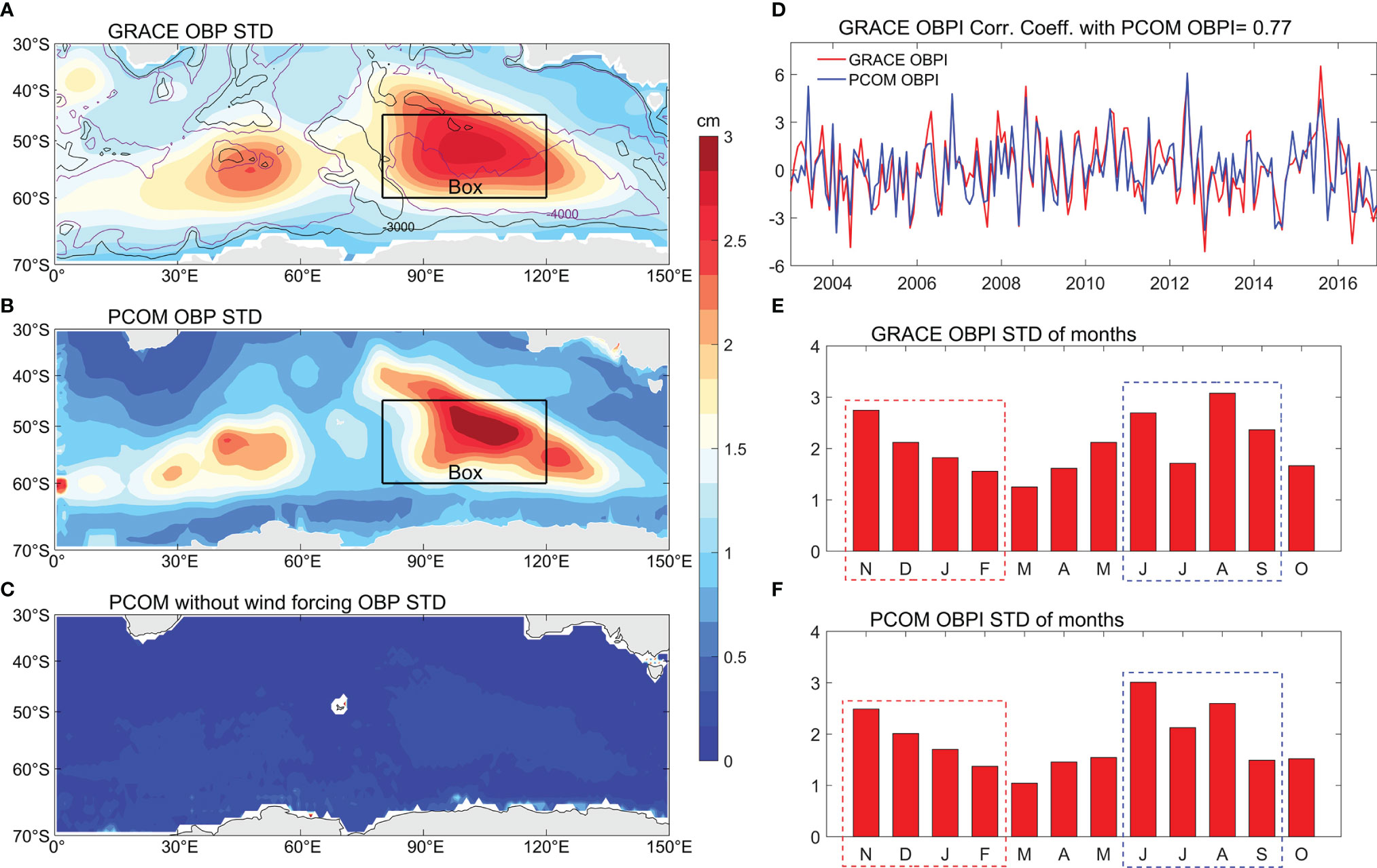
Figure 1 Standard deviation map of (A) GRACE OBP anomalies, (B) PCOM OBP anomalies with control runs and (C) PCOM OBP anomalies without wind forcing in the Southern Indian Ocean from 2003 to 2016. The contours represent isobaths from 3000 (black) to 4000 (purple) meters. (D) The GRACE OBP anomalies and PCOM OBP anomalies averaged in the black box (45°-60°S, 80°-120°E, unit: cm) with annual cycle removed, referred to as GRACE OBPI (red line) and PCOM OBPI (blue line), respectively. The standard deviation variation of (E) GRACE OBPI and (F) PCOM OBPI varies with month (unit: cm).

The OBP anomalies averaged in the region (45°–60°S, 80°–120°E; black box in Figure 1A) is considered as an index that measures the variability of the OBP in the Southern Indian Ocean. The OBP indices in the GRACE and PCOM control runs (hereafter referred to as the GRACE OBPI and PCOM OBPI, respectively) are shown in Figure 1D. The correlation coefficient between two OBPIs is 0.77 (significant at the 99% confidence level), and both GRACE OBPI and PCOM OBPI have a maximum amplitude above 6 cm. According to the monthly standard deviation of the GRACE OBPI and PCOM OBPI (Figures 1E, F), one can see that although the climatological annual cycle has been removed, they are relatively active during austral summer (NDJF) and winter (JJAS).

Figure 2 shows the empirical orthogonal function (EOF) analysis of monthly GRACE OBP anomalies in the Southern Indian Ocean (30°−70°S, 20°−130°E). EOF1 and EOF2 account for 42.8% and 15.6% of the total variance, respectively. The spatial structure of EOF1 is similar to the standard deviation map of the OBP in the Southern Indian Ocean (Figure 1A), and its corresponding principal component (PC) is closely related to the GRACE OBPI and PCOM OBPI (R = 0.94 and 0.72, respectively, both of which are significant at the 99% confidence level) during the period of 2003-2016. The spatial structure of EOF2 shows a dipole mode in the zonal direction, but the correlation coefficient between PC2 and GRACE OBPI is only 0.31, and that with PCOM OBPI is 0.22 (respectively, not significant at the 95% confidence level). Thus, the OBPI can be used to represent the temporal variations of EOF1 in both GRACE and PCOM control runs.

FIGURE 2

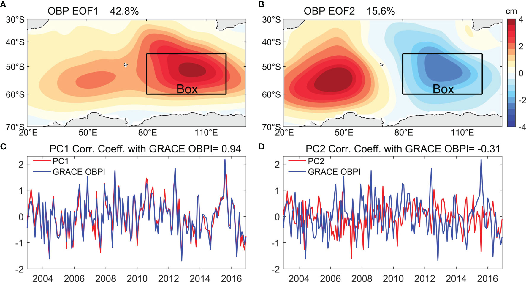
Figure 2 (A, B) First two EOF patterns of the GRACE OBP anomalies (with annual cycle removed) over the Southern Indian Ocean. (C, D) Corresponding normalized principal components (red line) and normalized GRACE OBPI (blue line).

Figure 3 shows the regression maps of OBP anomalies and Ekman transports upon the normalized OBPI in the GRACE and PCOM control runs during summer (NDJF) and winter (JJAS), when the OBP variations are active. The positive OBP in the Southern Indian Ocean is obviously accompanied by convergence of Ekman transport, which is consistent with previous findings (Gill and Niiler, 1973; Jing and Cheng, 2019; Cheng et al., 2021). It emphasizes the atmospheric source for the variability of OBP in the Southern Indian Ocean, which has not been well investigated in previous studies. Thus, the following study is focused on the possible source of wind forcing for the active OBP in the Southern Indian Ocean during summer (NDJF) and winter (JJAS).

FIGURE 3

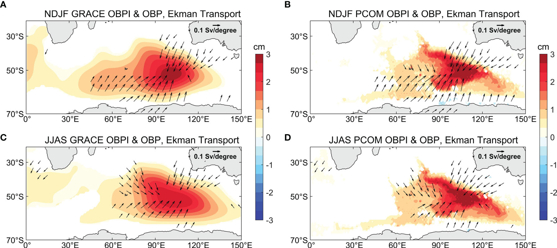
Figure 3 Regression coefficients of OBP anomalies (color) and Ekman transports (vector) on the (A) normalized NDJF-averaged GRACE OBPI and (C) normalized JJAS-averaged GRACE OBPI. (B) and (D) are identical to (A) and (C) but on PCOM OBPI. Only anomalies significant at the 95% significance level are shown.

3.2 Mechanisms of OBP Variability During Austral Summer and Winter

The regression maps of SLP anomalies and 10 m winds upon the normalized GRACE OBPI during summer (NDJF) and winter (JJAS) are shown in Figures 4A, C, respectively. There is a significant closed high pressure over the Southern Indian Ocean during both austral summer and winter. The anticyclone associated with anti-clockwise winds is favorable for convergence of Ekman transports there, which leads to enhanced OBP anomalies. Conversely, the SLP anomaly shows negative values to the south of 60°S and positive values around mid-latitudes. This result indicates the influence of the sea-saw pattern of SLP on the variability of the OBP in the Southern Indian Ocean, especially during austral summer (NDJF; Figure 4A), which is similar to the positive phase of SAM. Similar results are observed in the PCOM control runs (Figures 4B, D). To quantify the contribution of wind forcing to OBP, two idealized PCOM experiments are used (Figure 5). The experiments are forced by the regression wind anomalies (vectors in Figures 4A, C). The OBP anomalies diagnosed by PCOM are comparable to the regression maps (Figure 3). The results suggest that the wind anomalies are strong enough to trigger the interannual OBP variations in the Southern Indian Ocean.

FIGURE 4

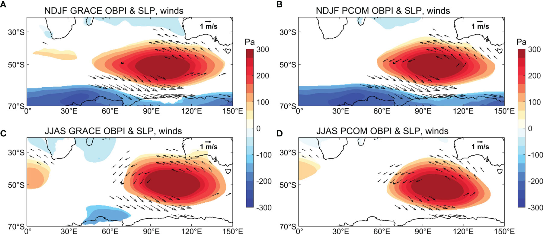
Figure 4 Regression coefficients of SLP anomalies (color) and 10 m winds (vector) on the (A) normalized NDJF-averaged GRACE OBPI and (C) normalized JJAS-averaged GRACE OBPI. (B) and (D) are identical to (A) and (C) but on PCOM OBPI. Only anomalies are significant at the 95% significance level are shown.

FIGURE 5

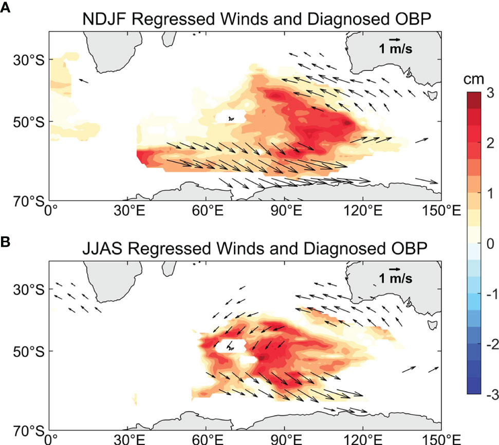
Figure 5 Ocean bottom pressure nomalies from two idealized PCOM experiments forced by the (A) regression wind anomalies in Figure Figures 4A, (B) regression wind anomalies in Figures 4C.

The correlation coefficients of the NDJF-averaged SAMI with concurrent GRACE OBPI and PCOM OBPI are 0.83 and 0.65 (Figure 6), respectively. The correlation between SAMI and OBP indices is also high during austral winter (JJAS; R = 0.69 and 0.64). All correlation coefficients are significant at the 95% confidence level, which suggests the crucial impacts of SAM on the simultaneous variability of OBP in the Southern Indian Ocean (black lines in Figure 6). The regression results of SLP anomalies, 10 m winds, OBP anomalies and Ekman transports on the normalized SAMI during summer (NDJF) and winter (JJAS) are shown in Figures 7A–D. As shown in Figures 7A, C, SAM can stimulate a high-pressure anomaly in the Southern Indian Ocean (approximately 45°S, 90°E), which contributes to the wind-driven convergence Ekman transport. As a result, both austral summer (NDJF) and winter (JJAS) OBP anomalies are enhanced in the Southern Indian Ocean during positive phase of SAM.

FIGURE 6

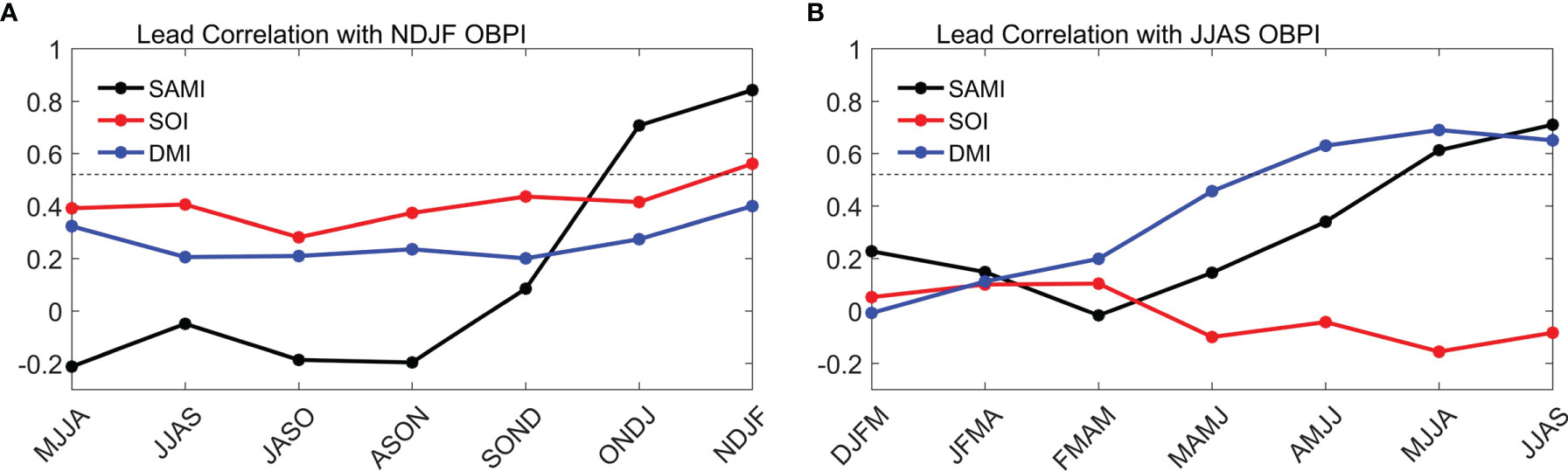
Figure 6 Lead correlation coefficients of the (A) NDJF-averaged GRACE OBPI and (B) JJAS-averaged GRACE OBPI with the 4-month averaged SAMI, SOI and DMI. The horizontal dashed line shows the 95% significance level.

FIGURE 7

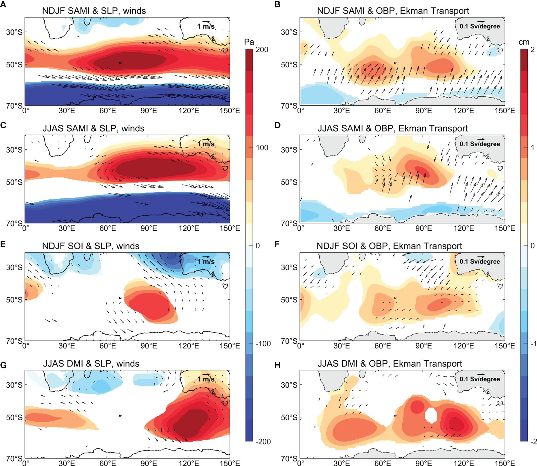
Figure 7 Regression coefficients of SLP anomalies (color) and 10 m winds (vector) on the (A) normalized NDJF-averaged SAMI, (C) normalized JJAS-averaged SAMI, (E) normalized NDJF-averaged SOI and (G) normalized JJAS-averaged DMI. (B, D, F, H) are identical to (A, C, E, G) but for OBP anomalies (color) and Ekman transports (vector). Only anomalies significant at the 95% significance level are shown.

Since some studies have suggested the influence of the tropics on SLP anomalies in the Southern Hemisphere (e.g., Ding et al., 2012), the lead correlation method is used to further determine the origin of OBP variability from the tropics. Due to the strong interannual variability of ENSO and IOD, the correlations between their indices and OBPI are checked. The correlation coefficients between 4-month running mean SAMI, SOI, DMI and the NDJF-averaged GRACE OBPI are shown in Figures 6A, B. One can see that the correlation coefficient of the GRACE OBPI with SOI is highest (R = 0.56, significant at the 95% confidence level) during austral summer (NDJF), but not significant during austral winter (JJAS). Additionally, the DMI can lead the JJAS-averaged GRACE OBPI by approximately 2 months with the highest correlation coefficient of 0.68 (significant at the 95% confidence level).

Such different results during summer (NDJF) and winter (JJAS) are mainly attributed to the seasonal phase lock of ENSO and IOD. The SLP anomalies associated with the Southern Oscillation (SO) have seasonal variability and show a positive center over the Southern Indian Ocean during austral summer (NDJF; Figures 7E, 8A–C). This result is consistent with Taschetto et al. (2011), who reported high pressure over the Southern Indian Ocean during ENSO. To further investigate the dynamical mechanism, we checked the regression of zonal mean vertical wind anomalies of 90°-120°E on the normalized NDJF-averaged SOI (Figure 9). We find that the positive phase of SO can cause an updraft in the tropics and downdraft in the extra-tropics, leading to an anomalous anticyclonic air circulation over the study area during austral summer. It benefits the convergence of Ekman transport and intensified the OBP there (Figure 7F). On the other hand, a positive IOD features an anomalously strong west–east SST gradient in the tropical Indian Ocean, and the SST signal can last until SON. Meanwhile, the SST-induced air convection stimulates a Rossby wave train at 200 hPa transferring from the tropical Indian Ocean to emanate poleward and eastward of the Southern Indian Ocean (Figures 10A, B), which is beneficial to the generation of an anomalous anticyclone in our study area (Figures 10C, 7G), resulting in the increase of OBP during austral winter (JJAS; Figure 7H). This result is consistent with McIntosh and Hendon (2018), who mentioned the specific path of the Rossby wave train and the high pressure anomalies in our study area. Therefore, SO plays an important role in OBP variability in the Southern Indian Ocean during austral summer (NDJF), while the IOD mode is crucial during austral winter (JJAS). Such results can also be reproduced by PCOM, which are not shown.

FIGURE 8

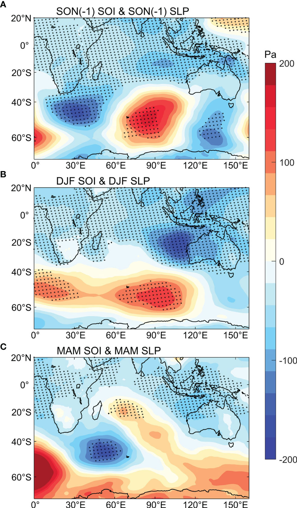
Figure 8 Regression coefficients of SLP anomalies on the (A) normalized SON-averaged (-1) SOI, (B) normalized DJF-averaged SOI and (C) normalized MAM-averaged SOI. Results significant at the 95% significance level are stippled.

FIGURE 9

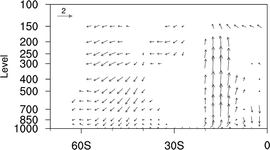
Figure 9 Regression coefficients of zonal mean vertical wind anomalies (vectors: m/s) of 90°-120°E on the normalized NDJF-averaged SOI. Only anomalies significant at the 95% significance level are shown.

FIGURE 10

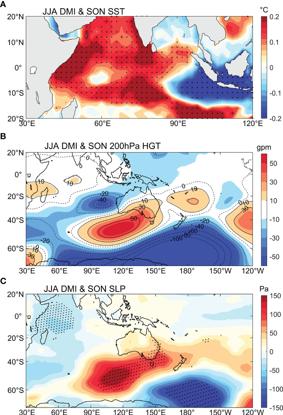
Figure 10 Regression coefficients of SON-averaged (A) SST anomalies, (B) 200 hPa geopotential height anomalies and (C) SLP anomalies on the normalized JJA-averaged DMI. SST and SLP anomalies which are significant at the 95% significance level are stippled.

Besides wind forcing, strong OBP centers are also related to closed planetary potential vorticity (i.e.,f/H with f being the Coriolis parameter and H the depth of the ocean) contours. There are closed planetary potential vorticity contours on the east and west sides of the Southern Indian Ocean (Figure 11), which can prevent the OBP signals from propagating outside the deep basin (Gill and Niiler, 1973; Cheng et al., 2021). Similar to the definition of OBPI, a simple index calculated with the OBP anomalies averaged in the southwestern Indian Ocean (50°–60°S, 40°–60°E) is named as OBPI-W. Figure 12 shows the regression maps of OBP anomalies, Ekman transports, SLP anomalies and 10 m winds on the normalized OBPI-W in the GRACE and PCOM control runs. Results show that the western energetic OBP center is also related to the wind anomalies caused by the SLP anomalies. Further analysis suggests that the OBP variability in the southwestern Indian Ocean is closely related to SAM, which can be seen from Figures 7A–D and it is weakly related to ENSO and IOD. SAM can explain 36% variation of OBP on interannual time scales, with the exception of IOD and ENSO (not shown).

FIGURE 11

Figure 11 Absolute value of planetary potential vorticity in the Southern Indian Ocean.

FIGURE 12

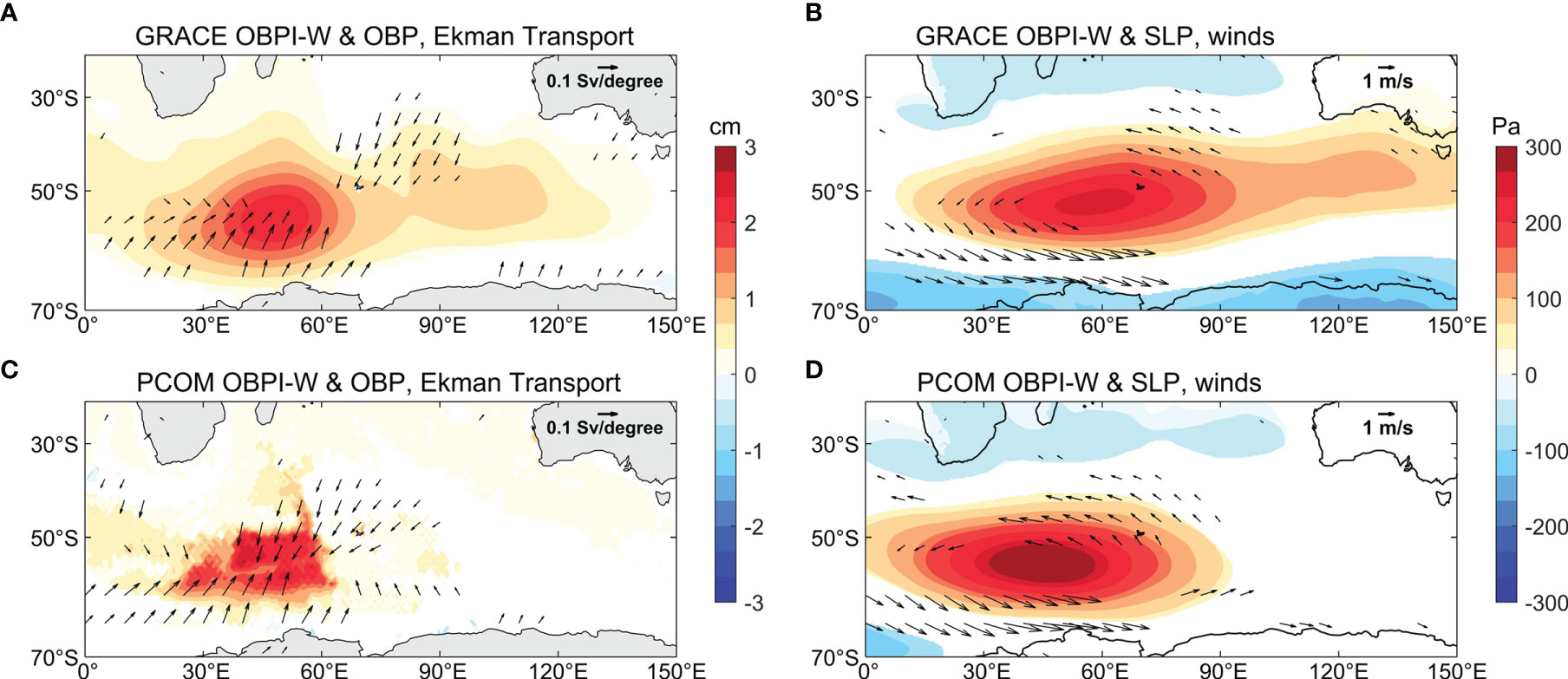
Figure 12 Regression coefficients of OBP anomalies (color) and Ekman transports (vector) on the (A) normalized GRACE OBPI-W and (C) normalized PCOM OBPI-W. (B, D) are identical to (A, C) but for SLP anomalies (color) and 10 m winds (vector). Only anomalies that are significant at the 95% significance level are shown.

4 Conclusions and Discussion

Using the GRACE observations and PCOM output, the characteristics and mechanisms of OBP variability in the Southern Indian Ocean on an interannual time scales are investigated in this study. There are two energetic OBP centers in the Southern Indian Ocean, the OBP anomalies averaged in the eastern center is considered as an index (OBPI) to measure the OBP variations, which is highly correlated with the PC of the OBP EOF1 (variance contribution is 42.8%). It can be found that OBP in the Southern Indian Ocean has significant interannual variability and is more active during austral summer (NDJF) and winter (JJAS). In addition to the effect of topography, wind forcing plays a dominant role in OBP variability by changing the local Ekman transport, which is consistent with previous studies (e.g., Gill and Niiler, 1973; Jing and Cheng, 2019; Cheng et al., 2021). The closed anticyclone associated with clockwise winds benefits the convergence of Ekman transport and enhances local OBP anomalies.

Our study preliminarily discussed the possible atmospheric sources of anticyclone anomalies in the Southern Indian Ocean. We find that the SLP anomalies are related to SAM, SO and IOD on interannual time scales. SAM can affect the OBP variability during the entire year, while SO and IOD only positively affect the OBP variability during austral winter (NDJF) and austral summer (JJAS), respectively. The positive phase of SO can cause an updraft in the tropics and downdraft in the extra-tropics, leading to an anomalous anticyclonic air circulation over the study area during austral summer. The SST-induced air convection associated with the positive phase of IOD forces a Rossby wave train transferring from tropical Indian Ocean to the south of Australia, resulting in an anomalous anticyclone appears in the Southeast Indian Ocean during austral winter.

In general, the results in this study help to understand the potential mechanisms of OBP fluctuations in the Southern Indian Ocean on interannual time scales. In this region, changes in OBP dominate the variations of sea level on interannual time scales (Figure 13). The correlation coefficient between observed sea level anomaly and OBP anomaly is 0.79 (significant at the 95% confidence level). Very good coherence also exists between them in the PCOM. Therefore, the study of OBP also can improve the understanding of the dynamics of sea level variations in Southern Indian Ocean.

FIGURE 13

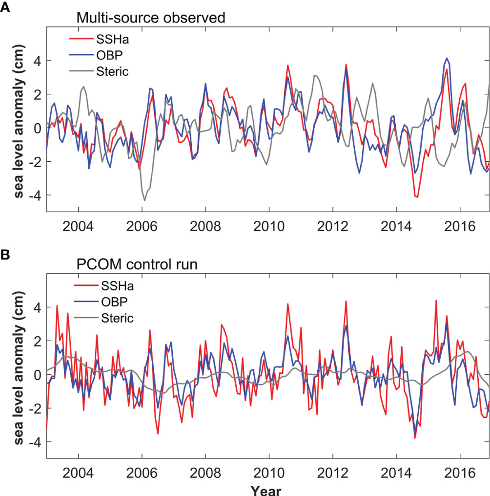
Figure 13 (A) The time series of sea surface height, OBP, steric sea level anomalies averaged in eastern southern Indian Ocean (45°-60°S, 80°-120°E, box in Figure 1A) derived from observations. (B) is same as (A) but for PCOM control run.

To date, the time series of GRACE satellite data is not sufficiently long for interdecadal analysis and long-term correlation between OBP variability and climate modes. Considering the important role of OBP in sea level change, long-term series observation data are of great significance for exploring the OBP mechanisms and predicting the sea level rise. PCOM well reproduces the observed OBP variations, because the wind forcing plays a crucial role in interannual variations of OBP in the Southern Ocean. To study the long-term change of OBP, the model must be further improved to include the effects of glaciers and rivers, which could improve the performance of the model to simulate and predict the impact of regional OBP variability on the global sea level find change.

Data Availability Statement

The original contributions presented in the study are included in the article/supplementary material. Further inquiries can be directed to the corresponding author.

Author Contributions

XC initiated the idea of this study. YN and XC wrote the manuscript. Other authors contributed to the data analysis and running the PCOM model. All authors contributed to the article and approved the submitted version.

Funding

This research was supported by the National Key R&D Program of China (2018YFA0605702) and the Natural Science Foundation of China (Grant nos. 41522601, 41876002, 41876224).

Conflict of Interest

The authors declare that the research was conducted in the absence of any commercial or financial relationships that could be construed as a potential conflict of interest.

Publisher’s Note

All claims expressed in this article are solely those of the authors and do not necessarily represent those of their affiliated organizations, or those of the publisher, the editors and the reviewers. Any product that may be evaluated in this article, or claim that may be made by its manufacturer, is not guaranteed or endorsed by the publisher.

References

Alexander M. A., Bladé I., Newman M., Lanzante J. R., Lau N. C., Scott J. D. (2002). The Atmospheric Bridge: The Influence of ENSO Teleconnections on Air-Sea Interaction Over the Global Oceans. J. Clim. 15, 2205–2231. doi: 10.1175/1520-0442(2002)015<2205:TABTIO>2.0.CO;2

CrossRef Full Text | Google Scholar

Boening C., Lee T., Zlotnicki V. (2011). A Record-High Ocean Bottom Pressure in the South Pacific Observed by GRACE. Geophys. Res. Lett. 38, 2–7. doi: 10.1029/2010GL046013

CrossRef Full Text | Google Scholar

Cabanes C., Huck T., Colin de Verdière A. (2006). Contributions of Wind Forcing and Surface Heating to Interannual Sea Level Variations in the Atlantic Ocean. J. Phys. Oceanogr. 36, 1739–1750. doi: 10.1175/JPO2935.1

CrossRef Full Text | Google Scholar

Cazenave A., Meyssignac B., Ablain M., Balmaseda M., Bamber J., Barletta V., et al. (2018). Global Sea-Level Budget 1993-Present. Earth Syst. Sci. Data 10, 1551–1590. doi: 10.5194/essd-10-1551-2018

CrossRef Full Text | Google Scholar

Chambers D. P. (2011). ENSO-Correlated Fluctuations in Ocean Bottom Pressure and Wind-Stress Curl in the North Pacific. Ocean. Sci. 7, 685–692. doi: 10.5194/os-7-685-2011

CrossRef Full Text | Google Scholar

Chambers D. P., Cazenave A., Champollion N., Dieng H., Llovel W., Forsberg R., et al. (2017). Evaluation of the Global Mean Sea Level Budget Between 1993 and 2014. Surv. Geophys. 38, 309–327. doi: 10.1007/s10712-016-9381-3

CrossRef Full Text | Google Scholar

Chambers D. P., Wahr J., Nerem R. S. (2004). Preliminary Observations of Global Ocean Mass Variations With GRACE. Geophys. Res. Lett. 31, 1–4. doi: 10.1029/2004GL020461

CrossRef Full Text | Google Scholar

Chambers D. P., Willis J. K. (2009). Low-Frequency Exchange of Mass Between Ocean Basins. J. Geophys. Res. Ocean. 114, 1–10. doi: 10.1029/2009JC005518

CrossRef Full Text | Google Scholar

Cheng X., Li L., Du Y., Wang J., Huang R. X. (2013). Mass-Induced Sea Level Change in the Northwestern North Pacific and its Contribution to Total Sea Level Change. Geophys. Res. Lett. 40, 3975–3980. doi: 10.1002/grl.50748

CrossRef Full Text | Google Scholar

Cheng X., Ou N., Chen J., Huang R. X. (2021). On the Seasonal Variations of Ocean Bottom Pressure in the World Oceans. Geosci. Lett. 8. doi: 10.1186/s40562-021-00199-3

CrossRef Full Text | Google Scholar

Dickey J. O., Bentley C. R., Bilham R., Carton J. A. (1997). Satellite Gravity and the Geosphere: Contributions to the Study of the Solid Earth and its Fluid Envelopes (Washington: National Acad. Press).

Google Scholar

Ding Q., Steig E. J., Battisti D. S., Wallace J. M. (2012). Influence of the Tropics on the Southern Annular Mode. J. Clim. 25, 6330–6348. doi: 10.1175/JCLI-D-11-00523.1

CrossRef Full Text | Google Scholar

Gill A. E., Niiler P. P. (1973). The Theory of the Seasonal Variability in the Ocean. Deep. Res. 20, 141–177. doi: 10.1016/0011-7471(73)90049-1

CrossRef Full Text | Google Scholar

Huang R., Jin X. (2002). Sea Surface Elevation and Bottom Pressure Anomalies Due to Thermohaline Frocing. Part I: Isolated Perturbations. J. Phys. Oceanogr. 32, 2131–2150. doi: 10.1175/1520-0485(2002)032<2131:SSEABP>2.0.CO;2

CrossRef Full Text | Google Scholar

Huang R., Jin X., Zhang X. (2001). An Oceanic General Circulation Model in Pressure Coordinates. Adv. Atmos. Sci. 18, 18–21. doi: 10.1007/s00376-001-0001-9

CrossRef Full Text | Google Scholar

Hughes C. W., de Cuevas B. A. (2001). Why Western Boundary Currents in Realistic Oceans are Inviscid: A Link Between Form Stress and Bottom Pressure Torques. J. Phys. Oceanogr. 31, 2871–2885. doi: 10.1175/1520-0485(2001)031<2871:WWBCIR>2.0.CO;2

CrossRef Full Text | Google Scholar

Hughes C. W., Smithson M. J. (1996). Bottom Pressure Correlations in the South Atlantic. Geophys. Res. Lett. 23, 2243–2246. doi: 10.1029/96GL01319

CrossRef Full Text | Google Scholar

Hughes C. W., Wunsch C., Zlotnicki V. (2000). Satellite Peers Through the Oceans From Space. Eos. (Washington. DC). 81, 68. doi: 10.1029/00EO00046

CrossRef Full Text | Google Scholar

Jin S. (2013). Satellite Gravimetry and Mass Transport in the Earth System. Obs. Model. Appl (London). 157–174. doi: 10.5772/51698171

CrossRef Full Text | Google Scholar

Jing X., Cheng X. (2019). Seasonal and Long-Term Variability of Ocean Bottom Pressure in the Indian Ocean. J. Trop. Oceanogr. 38, 10–17. doi: 10.11978/2018131

CrossRef Full Text | Google Scholar

Johnson G. C., Chambers D. P. (2013). Ocean Bottom Pressure Seasonal Cycles and Decadal Trends From GRACE Release-05: Ocean Circulation Implications. J. Geophys. Res. Ocean. 118, 4228–4240. doi: 10.1002/jgrc.20307

CrossRef Full Text | Google Scholar

Kanzow T., Flechtner F., Chave A., Schmidt R., Schwintzer P., Send U. (2005). Seasonal Variation of Ocean Bottom Pressure Derived From Gravity Recovery and Climate Experiment (GRACE): Local Validation and Global Patterns. J. Geophys. Res. C. Ocean. 110, 1–14. doi: 10.1029/2004JC002772

CrossRef Full Text | Google Scholar

Landerer F. W., Swenson S. C. (2012). Accuracy of Scaled GRACE Terrestrial Water Storage Estimates. Water Resour. Res. 48, 1–11. doi: 10.1029/2011WR011453

CrossRef Full Text | Google Scholar

Lee T., Hobbs W. R., Willis J. K., Halkides D., Fukumori I., Armstrong E. M., et al. (2010). Record Warming in the South Pacific and Western Antarctica Associated With the Strong Central-Pacific El Nio in 2009-10. Geophys. Res. Lett. 37, 1–6. doi: 10.1029/2010GL044865

CrossRef Full Text | Google Scholar

Makowski J. K., Chambers D. P., Bonin J. A. (2015). Using Ocean Bottom Pressure From the Gravity Recovery and Climate Experiment (GRACE) to Estimate Transport Variability in the Southern Indian Ocean. J. Geophys. Res. Ocean. 1–16, 4245–4259. doi: 10.1002/2014JC010575.Received

CrossRef Full Text | Google Scholar

Marshall G. J. (2003). Trends in the Southern Annular Mode From Observations and Reanalyses. J. Clim. 16, 4134–4143. doi: 10.1175/1520-0442(2003)016<4134:TITSAM>2.0.CO;2

CrossRef Full Text | Google Scholar

McIntosh P. C., Hendon H. H. (2018). Understanding Rossby Wave Trains Forced by the Indian Ocean Dipole. Clim. Dyn. 50, 2783–2798. doi: 10.1007/s00382-017-3771-1

CrossRef Full Text | Google Scholar

Peralta-ferriz C., Landerer F. W., Chambers D. P., Volkov D., Llovel W. (2017). Remote Sensing of Bottom Pressure From GRACE Satellites. US Clivar. Var. 15, 22–28.

Google Scholar

Piecuch C. G., Ponte R. M. (2014). Annual Cycle in Southern Tropical Indian Ocean Bottom Pressure. J. Phys. Oceanogr. 44, 1605–1613. doi: 10.1175/JPO-D-13-0277.1

CrossRef Full Text | Google Scholar

Piecuch C. G., Quinn K. J., Ponte R. M. (2013). Satellite-Derived Interannual Ocean Bottom Pressure Variability and Its Relation to Sea Level. Geophys. Res. Lett. 40, 3106–3110. doi: 10.1002/grl.50549

CrossRef Full Text | Google Scholar

Ponte R. M. (1999). A Preliminary Model Study of the Large-Scale Seasonal Cycle in Bottom Pressure Over the Global Ocean. J. Coast. Res. 104, 1289–1300. doi: 10.1029/1998JC900028

CrossRef Full Text | Google Scholar

Ponte R. M., Piecuch C. G. (2014). Interannual Bottom Pressure Signals in the Australian-Antarctic and Bellingshausen Basins. J. Phys. Oceanogr. 44, 1456–1465. doi: 10.1175/JPO-D-13-0223.1

CrossRef Full Text | Google Scholar

Price J. F., Weller R. A., Schudlich R. R. (1987). Wind-Driven Ocean Currents and Ekman Transport. Science 238, 1534–1538. doi: 10.1126/science.238.4833.1534

PubMed Abstract | CrossRef Full Text | Google Scholar

Qin J., Cheng X., Yang C., Ou N., Xiong X. (2022). Mechanism of Interannual Variability of Ocean Bottom Pressure in the South Pacific. Clim. Dyn. doi: 10.1007/s00382-022-06198-0

CrossRef Full Text | Google Scholar

Rintoul S. R. (2018). The Global Influence of Localized Dynamics in the Southern Ocean. Nature 558, 209–218. doi: 10.1038/s41586-018-0182-3

PubMed Abstract | CrossRef Full Text | Google Scholar

Tapley B. D., Bettadpur S., Watkins M., Reigber C. (2004). The Gravity Recovery and Climate Experiment: Mission Overview and Early Results. Geophys. Res. Lett. 31, 1–4. doi: 10.1029/2004GL019920

CrossRef Full Text | Google Scholar

Tapley B. D., Watkins M. M., Flechtner F., Reigber C., Bettadpur S., Rodell M., et al. (2019). Contributions of GRACE to Understanding Climate Change. Nat. Clim. Change 9, 358–369. doi: 10.1038/s41558-019-0456-2

CrossRef Full Text | Google Scholar

Taschetto A. S., Gupta A. S., Hendon H. H., Ummenhofer C. C., England M. H. (2011). The Contribution of Indian Ocean Sea Surface Temperature Anomalies on Australian Summer Rainfall During EL Niño Events. J. Clim. 24, 3734–3747. doi: 10.1175/2011JCLI3885.1

CrossRef Full Text | Google Scholar

Woodworth P. L., Vassie J. M., Hughes C. W., Meredith M. P. (1996). A Test of the Ability of TOPEX/POSEIDON to Monitor Flows Through the Drake Passage. J. Geophys. Res. C. Ocean. 101, 11935–11947. doi: 10.1029/96JC00350

CrossRef Full Text | Google Scholar

Yeh S. W., Kug J. S., Dewitte B., Kwon M. H., Kirtman B. P., Jin F. F. (2009). El Nĩo in a Changing Climate. Nature 461, 511–514. doi: 10.1038/nature08316

PubMed Abstract | CrossRef Full Text | Google Scholar

Zhang Y., Lin Y. H., Huang R. X. (2014). A Climatic Dataset of Ocean Vertical Turbulent Mixing Coefficient Based on Real Energy Sources. Sci. China Earth Sci. 57, 2435–2446. doi: 10.1007/s11430-014-4904-6

CrossRef Full Text | Google Scholar