Water temperature variability in the Coos Estuary and its potential link to eelgrass loss

Introduction

Estuaries act as mixing zones between oceanic and riverine waters, providing many ecosystem and cultural services (Milcu et al., 2013; Sherman and DeBruyckere, 2018; Zapata et al., 2018), and motivating numerous studies to examine the links between environmental conditions and ecosystem health (Costanza et al., 1997; Seppelt et al., 2011). In the Pacific Northwest (PNW; Figure 1), estuaries are influenced on the ocean side by the primarily wind-driven California Current System (CCS; Hickey and Banas, 2003). These winds driving the CCS along the west coast of North America are forced by atmospheric circulation related to the North Pacific High and the Aleutian Low, which vary seasonally. In the winter the Aleutian Low migrates southward, producing downwelling-favorable winds along the PNW, while in summer the North Pacific High migrates northward producing southward-directed upwelling-favorable winds (e.g., Huyer, 1983; Hickey and Banas, 2003; Davis et al., 2014). Upwelled waters on the PNW continental shelf are typically colder (Figure 1B), with higher salinity, higher nutrients and lower oxygen levels. During winter, storms produce episodic river discharge events that result in lower salinity, lower temperature and higher turbidity along the coast (Hickey and Banas, 2003; Huyer et al., 2007).

FIGURE 1

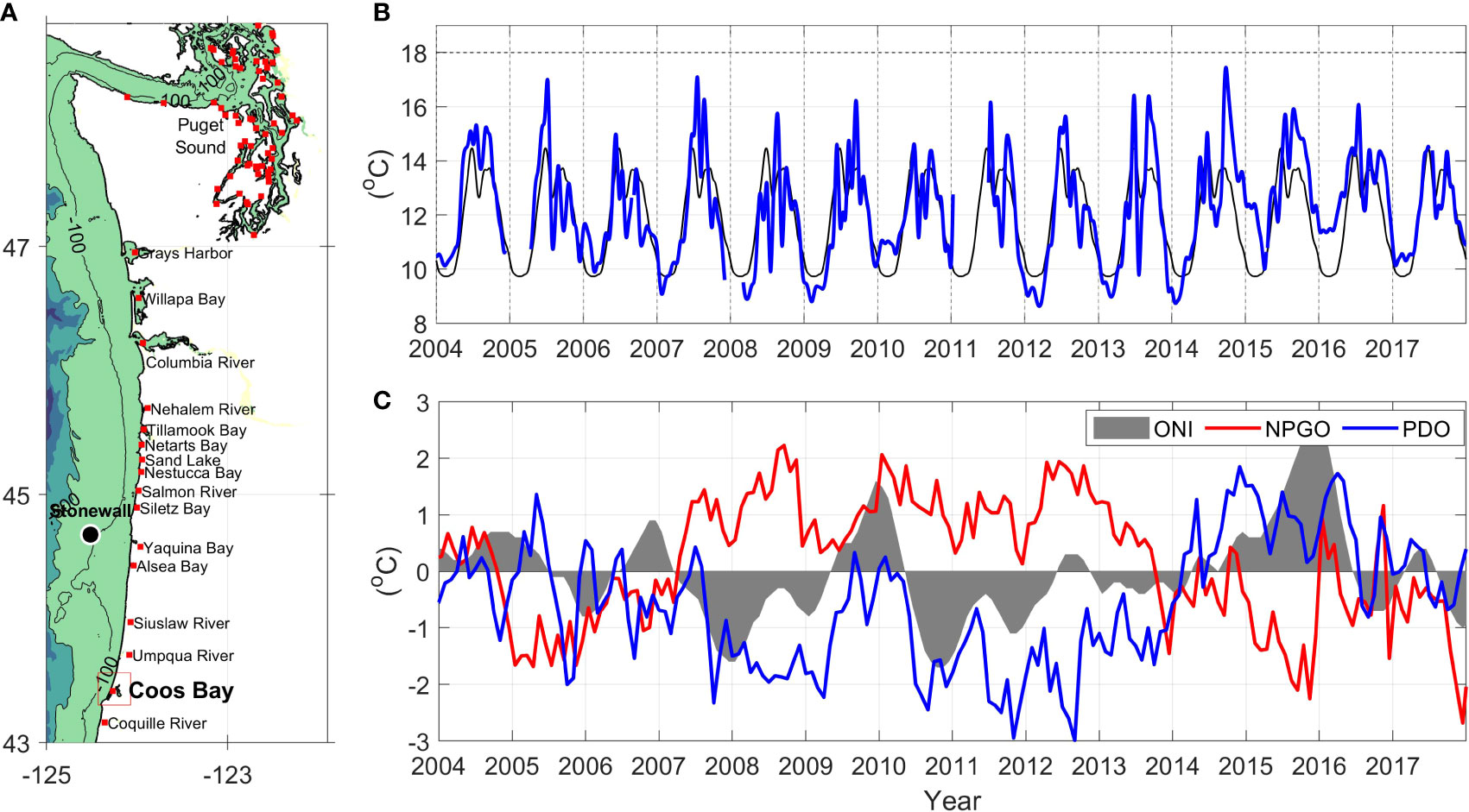
Figure 1 (A) Estuaries in the PNW where eelgrass (Zostera marina) is present, including our study area (Coos Bay). The Stonewall buoy is also shown as a black circle. (B) Water temperature at the Stonewall buoy with the climatological mean calculated for 2004-2014 (black) and the daily averaged values with a 30-day low pass filter (blue). (C) Basin scale indices (water temperature anomaly): Oceanic Niño Index (ONI; gray area), North Pacific Gyre Oscillation (NPGO; red line), and Pacific Decadal Oscillation (PDO; blue line).

The CCS exhibits significant interannual variability on top of its seasonal hydrographic changes (Figure 1C). These interannual variations are dominated by the El Niño Southern Oscillation (ENSO), where positive values of the Ocean Niño Index (ONI) are related to higher temperatures and sea level at the mouth of PNW estuaries (Wyrtki, 1984; Huyer et al., 2002). The triad of Sep-Oct-Nov 2014 ONI index registered SST anomalies greater than 0.5 °C in the Niño 3.4 region (5°N-5°S, 120°-170°W), which led to an officially declared El Niño in the Equatorial Pacific (https://origin.cpc.ncep.noaa.gov/). Though this first El Niño warm pulse was weak (0.5 °C in May-2014), another El Niño event produced SST anomalies of 4 °C in 2015, with maximum anomalies between Nov-2015 and Jan-2016. Positive anomalies were observed in this ENSO area until March-April-May 2016, with a peak of anomalies of 2.6 °C at the end of 2015. On decadal time scales, variations can be related to the Pacific Decadal Oscillation (PDO) and the North Pacific Gyre Oscillation (NPGO), which emerge as the first and second principal components of sea surface temperature and sea surface height, respectively (Di Lorenzo et al., 2008; Capotondi et al., 2019). The NPGO correlates with wind stress in the North Pacific, with weakened wind-driven upwelling occurring when the index is negative (Di Lorenzo et al., 2008). A positive PDO pattern, which is associated with a strengthened Alaskan gyre, is correlated to increased coastal upwelling between 38°N and 48°N (Chhak and Di Lorenzo, 2007; Di Lorenzo et al., 2008).

On top of these basin-scale patterns, marine heatwaves (MHWs) in the Eastern Pacific Ocean also contribute to interannual variations. MHWs are a result of decreased surface cooling in the Gulf of Alaska and decreased equatorward Ekman transport due to an atmospheric ridge (Di Lorenzo and Mantua, 2016; Capotondi et al., 2019). For example, during the winter of 2013, the MHW termed the “Blob” (Bond et al., 2015) was observed in the North Pacific and moved onto the shelf from Sep-2014 until Mar-2015, increasing SST more than 1.5 °C at the Stonewall buoy (Figure 1B). Positive anomalies (>1.5 °C) were observed at Stonewall again from Jul-2015 to May-2016 related to a second marine heatwave (Di Lorenzo and Mantua, 2016; Gentemann et al., 2017). Anthropogenic global warming is resulting in increased temperatures as well, which are predicted to increase stratification and reduce availability of nutrients higher in the water column, akin to the variations observed during El Niño years (Schneider, 1993; Di Lorenzo et al., 2009; Barnard et al., 2017). During 2014–2016, when the Coos Estuary showed anomalously warm waters (Shanks et al., 2020), the Equatorial Pacific was anomalously warm due to an El Niño event (Jacox et al., 2016), while MHWs were present on the PNW continental shelf.

The seasonal patterns in the continental shelf hydrodynamics influence the ecology of the PNW ocean and estuaries. For example, many local fish and invertebrates spawn in the winter to ensure the retention of pelagic eggs and larvae nearshore (Logerwell et al., 2003; Bi et al., 2011; Shanks et al., 2020). Plants are also influenced by the seasonal patterns in temperature. For example, eelgrass (Zostera marina) carries fewer leaves in the winter, while in the summer, they present a greater number of longer and thicker shoots (Phillips et al., 1983). This marine flowering plant forms broad meadows in intertidal and shallow subtidal flats, as well as fringe meadows on steeper shorelines, hence specific genotypes are selectively adapted to different habitats and environmental stressors (Phillips, 1984; Hessing-Lewis et al., 2011). Thom et al. (2003) showed the greatest densities of eelgrass in the Coos Estuary, OR, were found in the most marine-influenced sites. These sites had a smaller seasonal temperature range, while the stations further away from the mouth of the estuary were subjected to broader temperature ranges, higher turbidity, and lower salinity.

Many environmental parameters, outside a specific species-dependent range, can cause stress on the fauna and flora of estuaries, including salinity, water temperature, turbidity, light availability, air temperature, water velocity, and nutrient levels (Thom et al., 2003; Echavarria-Heras et al., 2006; Lee et al., 2007; Nejrup and Pedersen, 2008; Kaldy, 2012; Kaldy, 2014; Salo and Pedersen, 2014; Basilio et al., 2017; Daly et al., 2017; Magel et al., 2022). For example, declines in eelgrass populations have been observed in the PNW and were related to increased water temperatures after the 1997-1998 El Niño event (Thom et al., 2003). Water temperatures above 25°C can significantly reduce photosynthetic and respiration rates (Nejrup and Pedersen, 2008; Gao et al., 2017; Beca-Carretero et al., 2018), inhibit leaf growth (Zimmerman et al., 1989), as well as increase susceptibility to eelgrass wasting disease (Kaldy, 2014; Groner et al., 2021). As a response to warm seasons, Z. marina may respond by reproducing sexually through the production of flowers and seeds (Lee et al., 2007). These seeds can also be affected by temperature by changing the size and chemical composition (Jarvis et al., 2012; Delefosse et al., 2016), and if the temperature stress is perennial, the eelgrass beds may not be able to survive (Jarvis et al., 2012).

Here, we study the seasonal and interannual variability of water temperature within the Coos Estuary to explore its links with a recently observed decrease in eelgrass abundance. Using long-term observations, we evaluate the impact of the ambient ocean conditions, river discharge and atmospheric heat flux on the water temperature in the estuary. Our observations show that temperature varies locally and seasonally across specific regions of the estuary, much like the observed eelgrass declines, and is driven by a combination of basin scale variability and local conditions dictated by the strongly-forced estuary.

Study area

The Coos Estuary is located inshore of a narrow continental shelf south of Stonewall Bank (Hickey and Banas, 2003) and is the second largest estuary in Oregon in terms of area and volume (Figure 1). Water temperatures inside the Coos Estuary are significantly correlated with continental shelf values as measured by the Stonewall buoy (Strub et al., 1987; Miller and Shanks, 2004; Huyer et al., 2007). At the Stonewall buoy, temperature shows a seasonality related to the CCS: equatorward winds drive cold upwelled waters towards the coast during the summer, while during the winter southward winds produce downwelling accompanied with warmer waters. On top of this seasonality, several warm-water events have been registered at the Stonewall buoy, including El Niño events which produce 1-2°C anomalies (Huyer et al., 2002; Peterson et al., 2017) and MHWs, which in 2014 produced an anomaly of 7°C in 1 hour at the Stonewall buoy (Gentemann et al., 2017; Shanks et al., 2020). These ocean conditions set the boundary conditions at the mouth of PNW estuaries and can travel up-estuary at a rate on the order of 10 km d^-1, at least in the case of Willapa Bay (Hickey and Banas, 2003).

The propagation of oceanic signals into an estuary is produced by a combination of baroclinic, barotropic and diffusive processes, which depend on the geometry, depth, and forcing of each system. The main channel of the Coos Estuary (Figure 2) is annually dredged from the mouth to 24 km up-estuary near the Coos River entrance, to maintain 11 m of depth and 91 m of width (Eidam et al., 2020). Adjacent tidal flats, inlets and sloughs branch out of the main channel; these shallow areas range between 0.5 m above MLLW to 1.0 bellow MLLW of depth, extend approximately 15 km² and provide the primary habitat for Zostera marina (Emmett et al., 2000; Groth and Rumrill, 2009; Eidam et al., 2020). The main source of freshwater is the South Fork Coos River in the eastern portion of the estuary (Figure 2), which has a total discharge that ranges from 2 to 800 m³ s^-1, with maximum peaks related to winter storm events. Additionally, there are numerous other sources of freshwater, including the Winchester, Elliot and Joe Ney Creeks that feed into South Slough. South Slough is a shallow sub-estuary that trends southward about 3 km from the mouth of the main estuary, has a natural depth of 5 m in its un-dredged sinuous channel, and is home to the South Slough National Estuarine Research Reserve (SSNERR), which collects water quality and eelgrass data throughout the entire estuary.

FIGURE 2

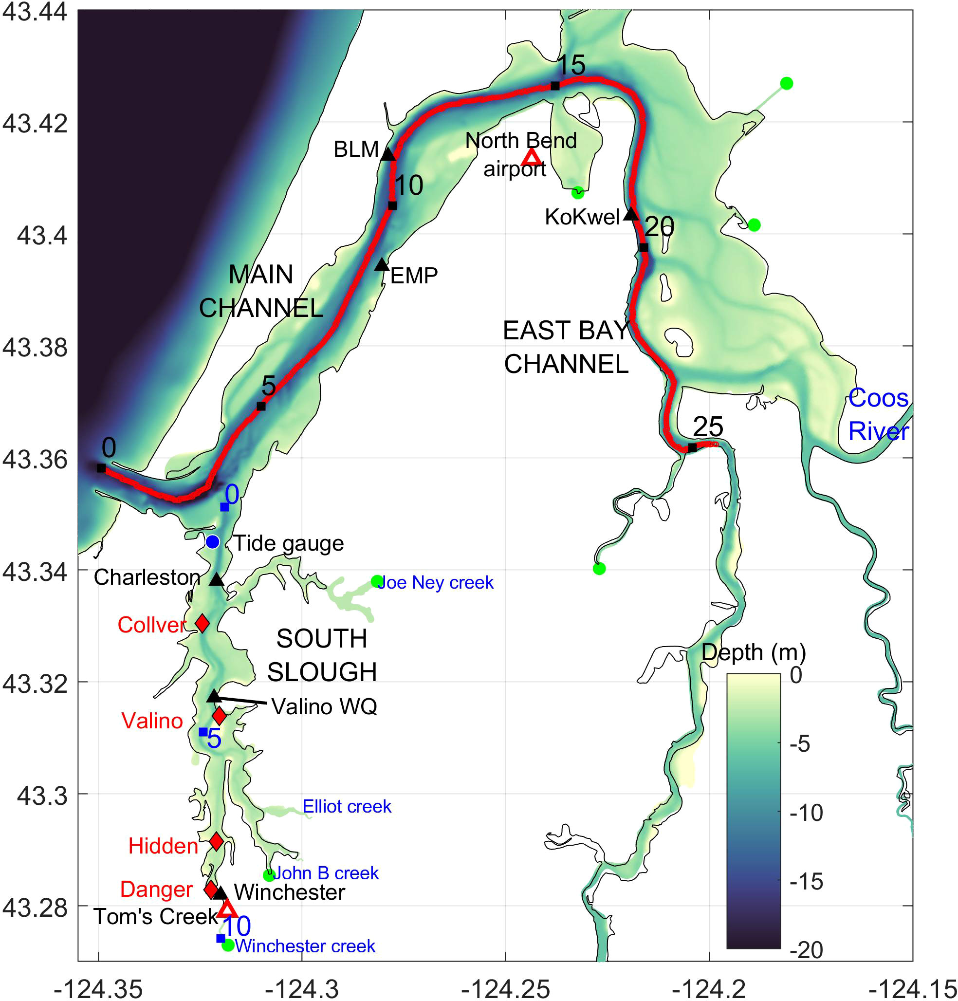
Figure 2 The Coos Estuary, showing bathymetry in meters below mean sea level (colored contours) and the location of water quality monitoring stations (black triangles), meteorological stations (red triangle), tide gauge (blue circle), freshwater sources (green circles), and eelgrass stations (red diamonds). Black numbers refer to distance (in km) from the mouth along the thalweg; blue numbers show distance (in km) from the intersection of South Slough with the main estuary.

The subtidal estuarine exchange flow in the Coos Estuary is relatively constant throughout the year as it is dominated by tides, with a small secondary increase in winter as river discharge ramps up (Conroy et al., 2020). The main semidiurnal tidal constituent, M_2, height amplitude is 0.8 m, with mean tidal currents of 1 m s^-1 resulting in a tidal excursion of 14 km (Baptista, 1989). Sutherland and O’Neill (2016) showed that the Coos Estuary has characteristics of a salt-wedge during high river discharges, a well-mixed estuary during low discharges, and a partially-mixed estuary during moderate discharge times. They also found that, as in other estuaries in the PNW, Ekman-driven upwelling moves high-salinity, low-temperature, low-oxygen waters into the estuary (Sutherland and O’Neill, 2016). Though estuaries are expected to be exporters of nutrients (e.g., Roegner et al., 2002; Roegner et al., 2011), Roegner and Shanks (2001) found that the Coos Estuary, specifically the seaward portion of South Slough, is an importer of nutrients in the summer, due to the close proximity of the coastal ocean.

Eelgrass, which plays a key role in the coastal zone worldwide (Phillips, 1984; Hosack et al., 2006; Lee and Brown, 2009), has decreased in abundance in PNW estuaries (Magel et al., 2022), including the Coos at one annually-sampled site. In the Coos, eelgrass is spatially variable, and estuary-wide eelgrass presence has been obtained through aerial photography and high density lidar intensity images from 2005 and 2016 with the aid of the US Environmental Protection Agency (EPA) and the Pacific Marine and Estuarine Fish Habitat Partnership (PMEP), respectively (Clinton et al., 2007; Sherman and DeBruyckere, 2018). In May 2005, false color, near-infrared aerial photography (Supplementary Figure 1A) revealed high eelgrass density in the Coos Estuary covering 24x10⁶ m² of total area. Higher density is observed in locations closer to the mouth of the estuary, where colder more saline oceanic waters flood the tidal flats (Thom et al., 2003). In July 2016, airborne, multispectral imagery was collected over Coos Bay that led to map of presence/absence of eelgrass beds (Supplementary Figure 1B). This 2016 survey revealed a decrease of eelgrass-covered area in the Coos Estuary, with higher presence in the main channel than in South Slough (Supplementary Figure 1B), despite the proximity of the sub-estuary to the mouth of the estuary and influence of coastal waters (Raimonet and Cloern, 2017). Previously, Thom et al. (2003) showed that stations in the Coos Estuary closer to the mouth had higher values of eelgrass density (100–200 shoots per m²) related to the influence of oceanic, low-turbidity waters, while stations farther away from the mouth of the estuary had smaller density, related to increased turbidity due to the input of freshwater. A similar result was found across multiple PNW estuaries by Magel et al. (2022). Thom et al. (2003) also suggested that eelgrass decline was correlated with anomalously warm waters during the 1997–1998 El Niño; the degree to which this happens again between 2014-2016 is the subject of this study (Figure 1). However, despite the proximity of South Slough to the mouth of the estuary, the spatial signature of eelgrass declines between 2005 and 2016 reveals that a simple picture of proximity to the ocean leading to loss does not hold, i.e., other factors influencing temperature along and across the estuary must play a role.

Methods

Environmental conditions

We obtain water property, sea level, river discharge and meteorological conditions from several monitoring stations located in the estuary (Figure 2 and Table 1). Inside South Slough, the Charleston Bridge, Valino Island and Winchester Arm stations are telemetered to provide near real-time data access by SSNERR (http://nvs.nanoos.org). Temperature, salinity and various other parameters, are measured automatically every 15 minutes at all stations (Figure 3). The instruments are maintained monthly to limit biofouling by SSNERR (NOAA National Estuarine Research Reserve System (NERRS), 2020).

TABLE 1

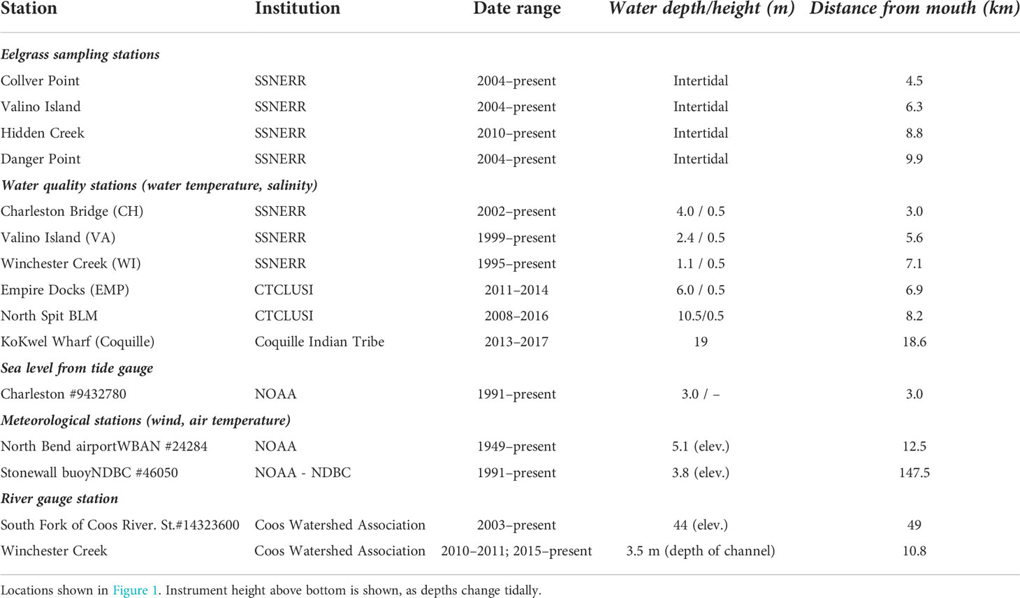
Table 1 Information on oceanographic and meteorological stations analyzed in this study.

FIGURE 3

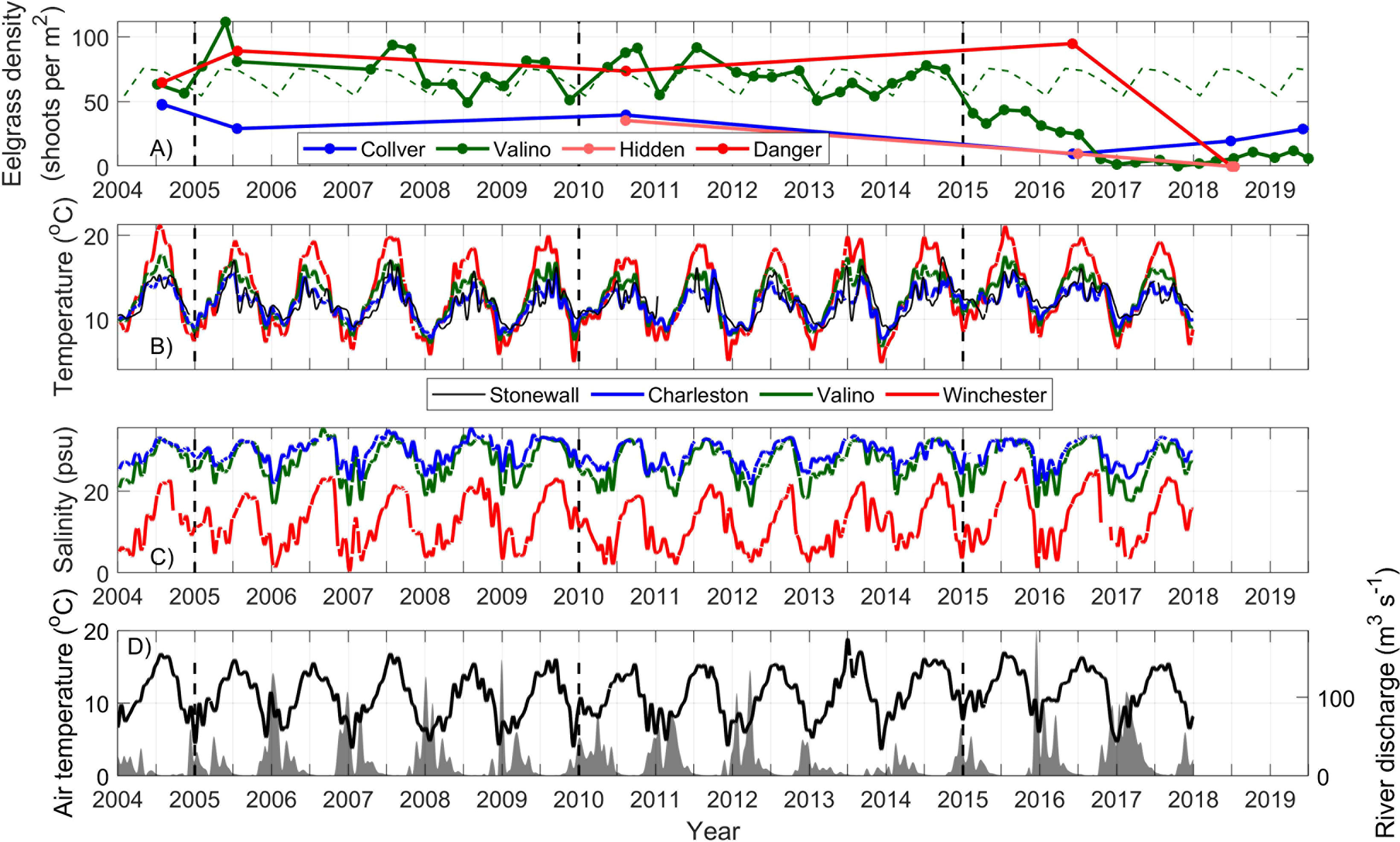
Figure 3 (A) Eelgrass density at 4 stations in South Slough. The 2004-2014 climatology for Valino is shown in broken green line. (B) Long-term hydrographic characteristics at 4 SSNERR stations, Charleston WQ (blue), Valino WQ (thick green), Winchester WQ (red) and the Stonewall buoy (black), showing low-pass filtered water temperature over 2014–2018. (C) same as in (B) but for salinity. (D) Air temperature at the North Bend Airport meteorological station (black) and South Fork of the Coos River discharge (gray). For locations, see Figure 2.

Meteorological data were obtained from stations both offshore and on land. Offshore wind data, taken to be representative of upwelling or downwelling conditions at the coast, are from the NOAA Stonewall Bank buoy (Figure 1), approximately 120 km north of the estuary. We use hourly wind data to calculate the along-shore north-south component of wind stress (Large and Pond 1981), given the wind speed at the height above ground from each station (Table 1). Surface water temperatures were also obtained from the Stonewall buoy at hourly intervals. On land, wind velocity data were extracted from a meteorological station at the North Bend Southwest Oregon Regional Airport (Table 1, location shown in Figure 2). The North Bend airport also provides air temperature, relative humidity, barometric pressure, total solar radiation and precipitation.

River discharge data from the South Fork Coos River gauge (Figure 2 and Table 1) from 2003 to present were used as a proxy for the variation in freshwater input to the estuary. Additionally, there are river discharge and water temperature data at Winchester Creek, the main source of freshwater entering the landward end in South Slough, available from 2011 and 2013-2016 (Figure 2 and Table 1). Hourly tidal height time series were obtained from a NOAA tide gauge in Charleston (Figure 2 and Table 1).

Heat budget

We use a heat budget approach to determine the total heat content of the volume of water of the estuary, from heat fluxes through the volume boundaries (Smith, 1983; Stevenson and Niiler, 1983). Here, we explore the heat budget of the Coos Estuary qualitatively, using a simplified heat budget for a shallow and vertically well mixed estuary,

$\begin{array}{ll}\frac{\partial T_{av}}{\partial t}+u_{av}\frac{\partial T_{av}}{\partial x}+Residual=\frac{Q_0}{\rho C_{p}h}& (1)\end{array}$

where T_av and u_av. are depth-averaged temperature and along-estuary horizontal current, respectively. We neglect several terms in the full heat budget, which are contained in the “Residual” term in Eq. 1 and are described next. Since surface to bottom differences in temperature in the Coos Estuary are out of phase with sea level differences, as well as with velocity (Roegner and Shanks, 2001; Conroy et al., 2020), we can assume heat divergence and entrainment are small. We also neglect the vertical heat flux through the sediment at the bottom, given the turbidity in the estuary as well as the amount of vegetation that both reduce the exchange of heat between the sediment and the water (Evans et al., 1998; McKay and Iorio, 2008).

This simplified heat budget, then, contains four terms: the heat storage, the along-estuary advective heat flux divergence, the residual term which includes the neglected terms, and on the right-hand side (RHS), the atmospheric heat flux. The storage of heat in the water column (first term in Eq. 1), is a partially measurable variable, since the measurements are obtained at a single depth (0.5 m). However, Sutherland and O’Neill (2016) show that in most of the profiles along the estuary, temperature isolines are nearly vertical, indicating well-mixed conditions. Hence, we assume that the point measurements represent the water column, though this assumption is most uncertain during high discharge (Sutherland and O’Neill, 2016).

The heat flux term is Q₀ which is the net surface heat flux, ρ is density averaged over the water column and C_p is the specific heat of sea water, both calculated as a function of temperature and salinity, and h is the time-varying water depth. Q₀ may be decomposed into the incoming solar short-wave radiation, outgoing longwave radiation, latent heat exchange due to evaporation or condensation, sensible heat exchange at the surface and heat exchange due to precipitation (assumed here to be negligible). Shortwave and longwave radiation, were obtained from the NCEP-NCAR Reanalysis (Kalnay et al., 1996) at the land location closest to the Coos Estuary (123.75°W, 44.7611°N). Sensible and latent heat fluxes are estimated using bulk formulae from the MATLAB Air-Sea toolbox (https://github.com/sea-mat/air-sea), using the water quality parameters at Valino WQ and the meteorological observations at the North Bend airport.

The second term in Eq. 1 represents the horizontal advective flux divergence of heat past a point in the along-estuary direction. We assume the across-estuary advective heat flux divergence is small, since the across-channel velocity is 2 magnitudes smaller than the along-estuary component (Roegner and Shanks, 2001; Conroy et al., 2020). Hence, it is included in the “Residual” term of Eq. 1. We calculate the along-estuary advective component of the heat budget by assuming that the heat storage (first term in Eq. 1) minus atmospheric heat flux (RHS in Eq. 1), is dominated by the along-estuary advective heat fluxes plus the residual. These horizontal heat flux divergences depend on the temperature gradient and velocity, which change due to the influence of the oceanic and riverine end-members.

Eelgrass (Zostera marina) in the Coos Estuary

Changes in the environmental conditions of an estuary have been observed to modify the seasonal trends of Zostera marina (Table 2). Due to the observed response of Z. marina to temperature, salinity and turbidity (Table 2), we use eelgrass as a proxy of response to environmental stressors in the Coos Estuary. The availability of observations and the importance of eelgrass to the ecosystem here and worldwide (e.g., Short and Coles, 2001) make it a critical species to examine. Table 2 synthesizes the current literature on temperature, salinity and turbidity on eelgrass density in estuaries in the PNW. Generally, warmer waters and waters with salinity outside an optimal range stress the eelgrass along the west coast. Although sediment also plays a role in eelgrass health, it is beyond the scope of variables we explore here.

TABLE 2

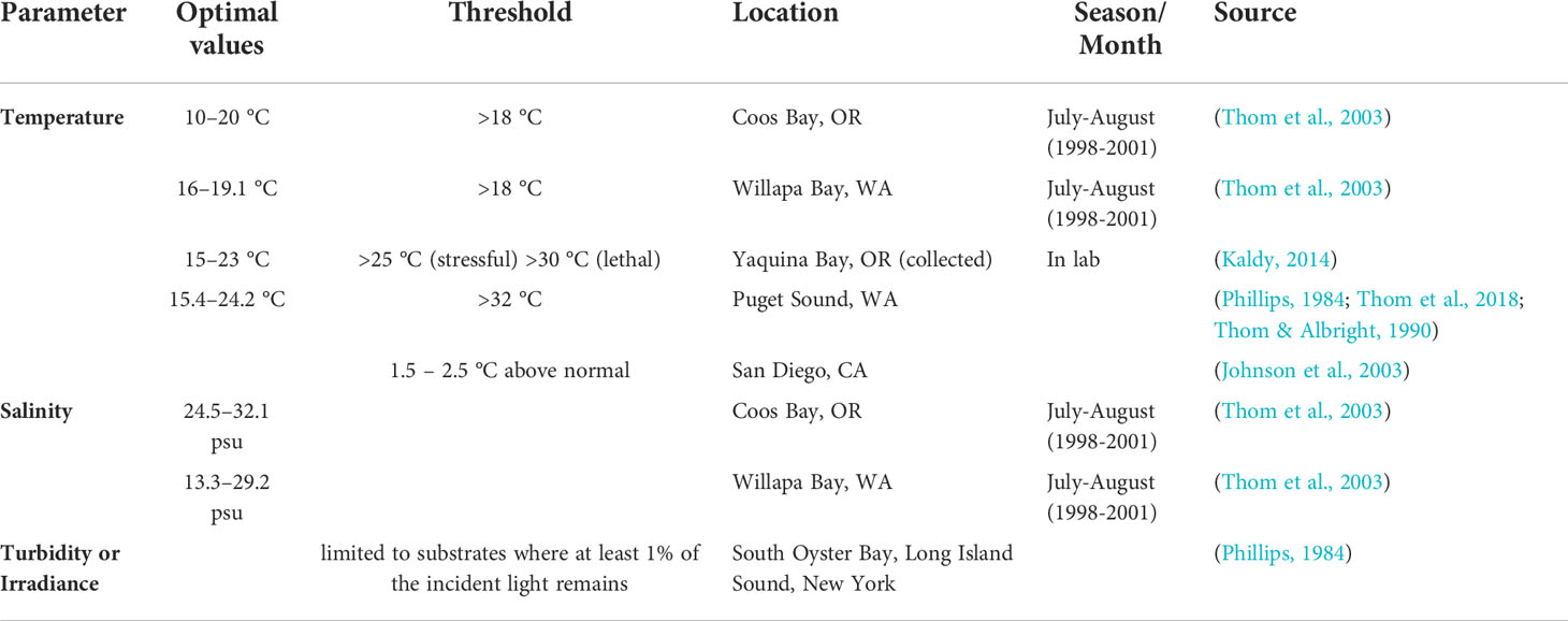
Table 2 Temperature, salinity and turbidity optimal physiological values and thresholds for the survival of Zostera marina in the Pacific Northwest.

SSNERR surveys eelgrass in the Coos Estuary, including quarterly to annual monitoring of percent cover, shoot density, canopy height and flowering shoot counts at 4 locations in South Slough (Table 1). Collver Point, Valino Island, Hidden Creek, and Danger Point, are sampled using SeagrassNet and NERRS biomonitoring protocols (Short et al., 2006). Eelgrass characteristics are sampled at 0.25 m² quadrats along permanent transects during low tides (Supplementary Figure 2). From 2004 to 2015, Valino Island transects contained 12 plots, and from 2016 to present 6 plots were added to the low and mid transects for a total of 18 plots.

Climatology and statistics

In order to compare the oceanographic and meteorological conditions of the Coos Estuary between 2014-2016 with the years before the observed eelgrass decline, we used the available data from 2004-2014 to calculate daily averages and standard deviations. Once the daily climatology was calculated, event-driven variability was filtered out by using a low-pass 30-day filter. Correlations between time series were calculated at different time lags, with significance level of 95%, using the large N (number of observations) approximation ${\widehat{\rho }}_{crit}\left(\alpha ,N\right)=\frac{q_t\left(\frac{\alpha }{2},N-2\right)}{\sqrt{N}}$, where q_t refers to the Student’s-t distribution with N-2 degrees of freedom, and α s the lower-tail confidence region, in our case 0.05. The water-year climatological cumulative river discharge was calculated from October 1^st to September 30^th, from 2004 to 2014. We define dry conditions in the estuary to be values below 95% of the climatological cumulative discharge value.

Results

Climatological environmental conditions in the Coos Estuary

Water temperature and salinity levels in the Coos Estuary are influenced by the atmosphere (wind and heat fluxes), ambient ocean conditions, and river discharge (Figure 3). During the winter, storms produce enhanced northward winds locally over the estuary (Figure 4). These same storms bring rain, increasing river discharge into the estuary episodically (Figure 4). Over the climatological period examined here (2004-2014), river discharge between November and May reached an average of 32 m³ s^-1 (although peaks in distinct years show much higher individual event magnitudes), after which is a dry period between June and October, where the average discharge decreased by an order of magnitude to 3.2 m³ s^-1 (Figure 4D). The average water-year cumulative discharge calculated for the South Fork Coos River is 6330 m³ s^-1. In a typical year, 90% of this cumulative discharge is accumulated between November and April.

FIGURE 4

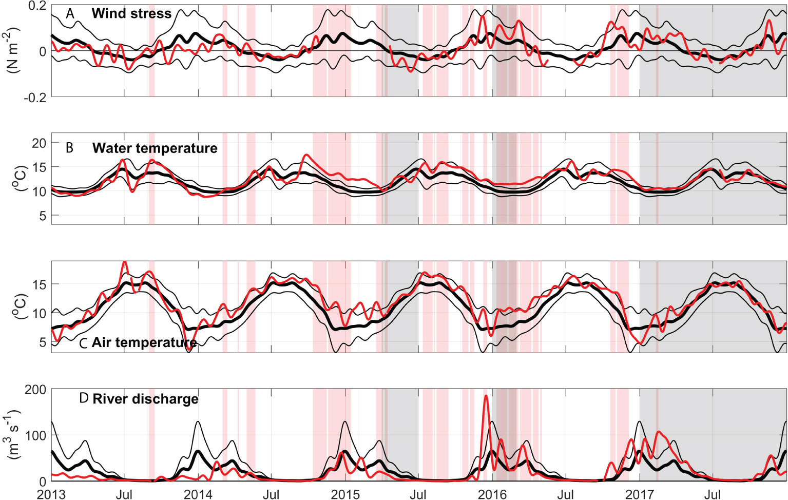
Figure 4 Environmental conditions outside the estuary during 2013-2017. (A) Daily averages with a 30-day low pass filter of North-South wind stress (N m^-2) from the North Bend Airport meteorological station (red lines) showing 2004-2014 climatological mean calculated for 2004-2014 (thick black lines), thin black lines show ±1 standard deviation. Vertical red bands show periods in which water temperature at Charleston WQ is 1 standard deviation above the 2004-2014 climatology (Figure 6). Vertical gray bands show periods in which eelgrass density at Valino is at least 1 standard deviation below the 2004-2014 climatology. (B) same as (A) but for surface water temperature (°C) at the Stonewall buoy, (C) same as (A) but for air temperature (°C) at the North Bend Airport meteorological station, (D) same as (A) but for South Fork Coos River discharge (m³ s^-1).

During the dry summer, air temperature reached maximum values of 15.2°C at the North Bend airport station, while in winter, values below 7 °C were recorded (Figure 4C). Outside the estuary, water temperatures at the Stonewall buoy location (Figure 4B) showed a similar pattern of seasonal variability: during the summer, temperatures increased, averaging 13 °C, albeit with event-driven decreases in temperature between July and September when upwelling brings colder waters to the coast. During the winter, colder water temperatures were observed at Stonewall, averaging 10 °C, and related to wintertime atmospheric heat loss.

Subtidal data from the Coos show that estuarine temperature is strongly correlated to the temperature variability on the nearby continental shelf (ocean end-member), but the correlation weakens with distance from the mouth (Supplementary Figure 3). Additional spatial variability is induced by the heterogenous input of freshwater: the main estuary receives the largest magnitude sources of river water (>10 freshwater sources) while South Slough has fewer sources with relatively smaller magnitudes (374 m³ s^-1 for the entire estuary, 8.8 m³ s^-1 for South Slough).

Inside the estuary, the 2004-2014 temperature climatology shows maximum values between July and October (Figure 5), which coincides with the highest air temperature values (Figure 4C) and reduced freshwater input (Figure 4D). The highest water temperatures were observed in stations further away from the mouth (KoKwel, 18 °C; and Winchester, 18.4 °C) during this season (Figure 5). Salinity was also high during the dry summer period with maximum values at the station closest to the mouth (Charleston, 29.2 psu). Winchester Creek data (Figure 6) showed that river temperature increases during the summer, yet remains ~2 °C cooler than both the Valino and Winchester locations in the estuary. At the end of the dry period, before freshwater increases, Charleston WQ (station closest to the mouth of the estuary) registered temperatures up to 3.5 °C colder and 9.6 psu saltier than Winchester WQ (station furthest up-estuary in South Slough), due to the influence of upwelling on the coastal ocean. Valino WQ (station located mid-estuary in South Slough) also registered the influence of cold salty upwelled waters, while Winchester WQ and Winchester Creek temperature continued to increase (Figure 5).

FIGURE 5

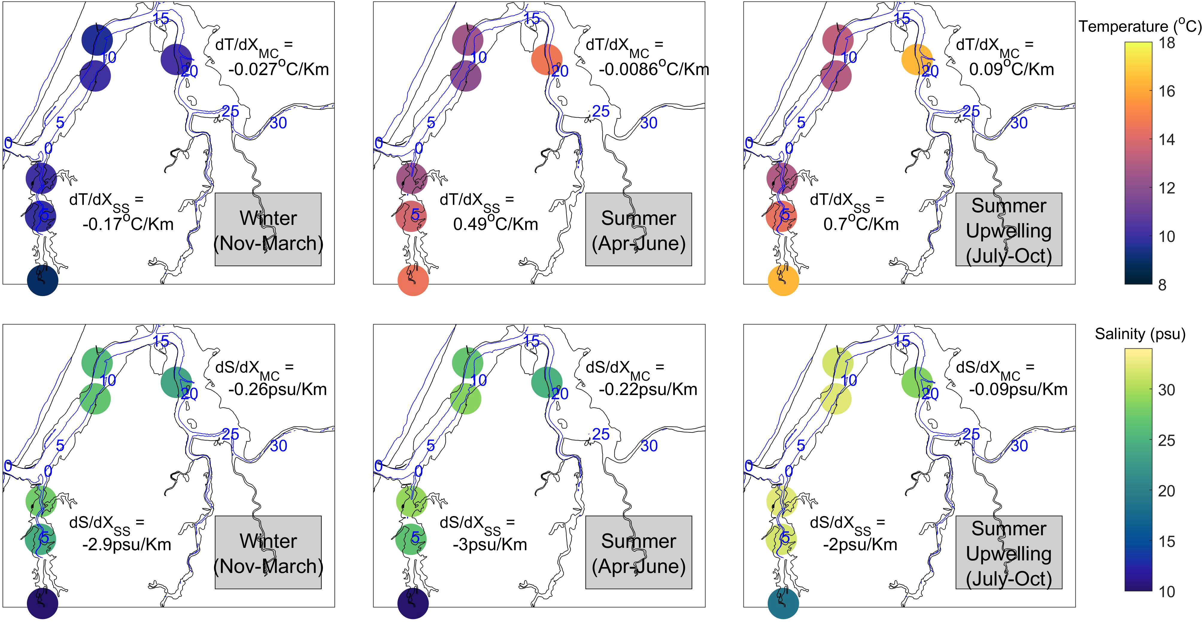
Figure 5 Spatial distribution of temperature (top plots) and salinity (bottom plots) 2004-2014 climatology derived at stations inside the Coos Estuary during Winter (left), Summer (middle) and Upwelling (right) time periods. Blue numbers refer to distance (km) from the mouth along the thalweg in the main channel and along the channel in South Slough.

FIGURE 6

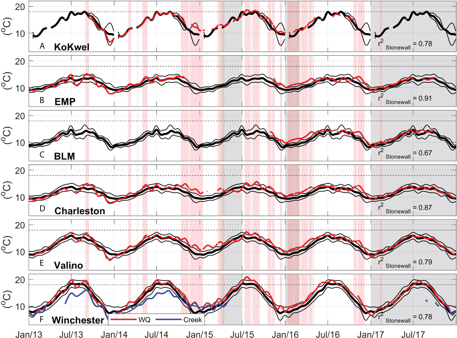
Figure 6 Coos Estuary water temperature during 2013-2017, thick black lines show 2004-2014 climatological mean, thin black lines show +/- 1 standard deviation, thin red line shows daily averages with a 30-day low pass filter. Red bands show periods in which water temperature at Charleston WQ is 1 standard deviation above the 2004-2014 climatology (black line in Figure 6D). Gray bands show periods in which eelgrass density at Valino is below the 2004-2014 climatology by one standard deviation. Correlation between Charleston WQ and the Stonewall buoy shown in text (significance level = 0.04). (A) KoKwel Wharf, (B) EMP, (C) BLM, (D) Charleston, (E) Valino and (F) Winchester WQ and Winchester Creek (blue). 18 °C eelgrass temperature threshold in broken black line for reference.

The rainy period, from November to March, was characterized by colder waters in Winchester Creek (Figure 6F). During this season all stations had similar temperatures (Figure 5), with even lower peaks during increases in discharge (Figure 4B). Due to the increase in freshwater input, salinity decreases, with lowest values in the stations closest to the river mouths (Winchester and KoKwel Wharf, and the eelgrass stations of Danger and Hidden). Despite KoKwel Wharf being closer to the input of freshwater from Coos River, temperature is slightly higher than BLM (10.2 °C, Figure 5). Long time series for the EMP, BLM, and KoKwel Wharf WQ stations are not available. However, existing data from 2013-2016 (Figures 6A–C) shows the strong seasonal pattern of temperature and salinity in these stations within the main channel. Salinity is highest at EMP, the station closest to the mouth, while KoKwel Wharf (closer to the main freshwater source) responds with greater amplitude variations to storm events (i.e., much fresher during February).

A few stressful years

A combination of anomalous atmospheric and oceanic processes occurred in the PNW from late 2013 until 2017: during the winter of 2013, “The Blob” was observed in the North Pacific due to a high-pressure system, moving onto the shelf from Sep-2014 until Mar-2015, increasing sea surface temperature more than 1.5 °C, i.e., the eelgrass threshold (Figure 1B). At the end of 2014, a strong El Niño event was registered in the Equatorial Pacific (up to 2.6 °C anomalies by the end of 2015, Figure 1C), influencing the PNW with warm anomalies of more than 1.5°C from Jul-2015 to May-2016, with additional input of heat due to another marine heatwave (Figure 1B). These anomalies would exceed the temperature stress threshold for eelgrass in the PNW (Table 2).

The persistent high-pressure also impeded the arrival of winter storms in 2013-2014, reducing river discharge and increasing air temperature at the estuaries in the PNW (Wang et al., 2014). During the winter of 2013-2014, the PNW experienced drought conditions reflected in the below-average water-year cumulative discharge at the South Fork Coos River location: 3240 m³ s^-1 during 2013, and 4750 m³ s^-1 during 2014, only 50% and 71% of the 2004-2014 climatological cumulative of 6330 m³ s^-1, respectively (Figure 4D). Lower river discharge is also related to the higher-than-average salinity during 2013 and 2014 (Figure 7). During this warm period, the Coos Estuary experienced extended time periods with water temperature ≥1.5°C than the mean: Charleston WQ registered 107 of the anomalously warm days during 2014, 116 days in 2015 and 146 days in 2016 (Supplementary Figure 4, calculated using the low-pass filtered data). The intrusion of anomalously warmer water in the Coos Estuary is especially noticeable during the Fall and Winter of 2014–2016 (Figure 6). In fact, of the days ≥1.5 °C the mean, 80% occurred during the winter months of October to December. In Oct-2014, water temperature registered 1 standard deviation above the mean at KoKwel Wharf, Charleston, Valino and Winchester, until the following Apr-2015. From Jul-2015 until May-2016, anomalously warm waters were again observed, with only short periods within 1 standard deviation of the mean. Despite the proximity of Valino WQ and Winchester WQ to the ocean boundary (5.6 and 7.1 km respectively, Figure 2), these stations showed a greater number of days with temperature anomalies above 1.5 °C in 2013-2016 compared to other water quality stations at similar or greater distance (Supplementary Figure 4), suggesting local estuarine dynamics are important. Winchester Creek also showed waters 2°C warmer than its 2004-2014 climatology in 2015, when discharge values were close to normal (Figure 6F). These temperatures were close to the estuarine water quality station at Winchester, during the rainy winter season of 2015 (Figure 6F).

FIGURE 7

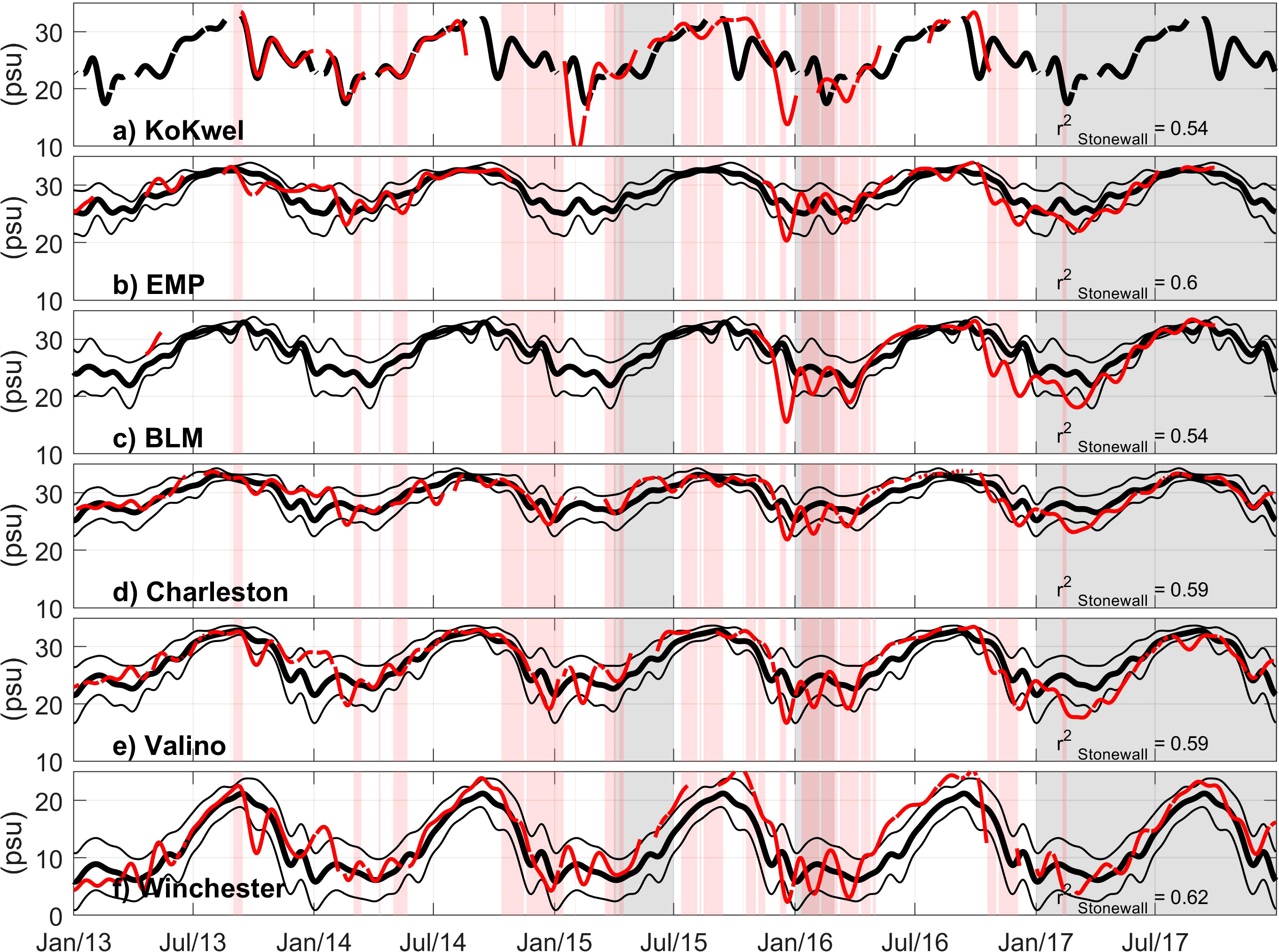
Figure 7 Coos Estuary salinity during 2013-2017, thick black lines show 2004-2014 climatological mean, thin black lines show ±1 standard deviation, thin red line shows daily averages with a 30-day low pass filter. Red bands show periods in which water temperature at Charleston WQ is 1 standard deviation above the 2004-2014 climatology (black line in Figure 6D). Gray bands show periods in which eelgrass density at Valino is below the 2004-2014 climatology by one standard deviation. Correlation between Charleston WQ and the Stonewall buoy shown in text. (A) KoKwel Wharf, (B) EMP, (C) BLM, (D) Charleston, (E) Valino and (F) Winchester WQ.

Heat budget in the Coos Estuary

The heat budget decomposition shows that heat storage (Figure 8A) is very small with no seasonal pattern. The net surface heat flux (Figure 8B), Q₀ , decomposed into the incoming solar short-wave radiation, outgoing longwave radiation, latent and sensible heat exchange at the surface, is highest in the summer and becomes negative in the winter, representing heat loss. Shortwave and longwave radiation have the greatest magnitudes, with values that fluctuate seasonally between 250 and 50 W m^-2 (shortwave) and -90 and -50 W m^-2 (longwave). Sensible and latent heat, though smaller, also show a seasonal pattern with positive values in July and August, related to wind and the air-sea temperature difference. Compared to the 2004-2014 climatology, Q₀ during 2014–2016 was anomalously positive (when data are available), mainly due to the shortwave radiation from March to July in those years, and parallels the anomalously high air temperature (Figure 4C).

FIGURE 8

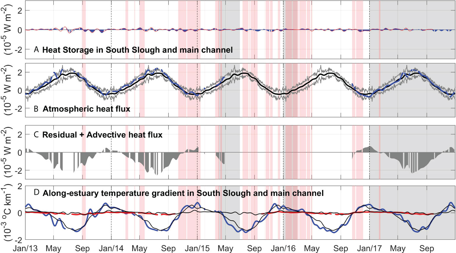
Figure 8 Heat budget components in the Coos Estuary during 2013-2017. (A) Heat storage in South Slough (blue) and the main channel (red). (B) Atmospheric heat flux using data from the Valino water quality station. (C) Residual + Advective heat flux (Heat storage minus Atmospheric heat flux), and (D) Along-estuary temperature gradient in South Slough (Charleston to Winchester) in blue and in the main channel (Charleston to KoKwel Wharf) in red. Positive ∂T_av/∂x indicates that the station closest to the ocean is warmer than the station furthest up-estuary. Red bands show periods in which water temperature at Charleston WQ is above the 2004-2014 climatology +1 standard deviation (Figure 6). Gray bands show periods in which eelgrass density at Valino is below the 2004-2014 climatology by one standard deviation.

The 2004-2014 climatology of along-estuary advective heat flux divergence, which depends on the temperature gradient and velocity, shows a strong seasonal pattern mostly in South Slough (between Charleston and Winchester WQ stations, 4.1 km apart), while the main channel (between Charleston and BLM WQ stations, 7.3 km apart) shows a smaller seasonal gradient (Figure 8). Stronger differences between Charleston and Winchester are observed during the dry season (up to -7 °C in late July), due to minimal river discharge and cooler upwelled waters on the oceanic side. In the winter, positive values of $\frac{\partial T_{av}}{\partial x}$, are observed in South Slough, when cooler river discharge closer to Winchester WQ reduces temperature there (Figure 6D) while the oceanic values vary relatively little. Water temperatures at Valino are significantly correlated (r² = 0.62) to the along-estuary temperature gradient calculated here, with a change in sign of $\frac{\partial T_{av}}{\partial x}$ at 11.6 °C. Our data shows that during the dry seasons of 2014–2016 (Figure 8D), the temperature gradient was stronger (more negative, especially in 2015–2016), due to warmer waters in the oceanic end member. This is observed in both South Slough (r²=0.6, Stonewall warmer 43 days before South Slough $\frac{\partial T_{av}}{\partial x}$) and in the main channel. During the rainy season, the temperature gradient is usually driven by increased discharge due to storm events. In the estuary, discharge from the Coos River increases 18 days before the along-estuary temperature gradient changes sign to positive values at South Slough ($\frac{\partial T_{av}}{\partial x}$ r²=0.6; Figure 4D). In 2013-2014, drought-induced reduced river discharge (Figure 4) would have decreased the advective export of water, while in 2014–2016 closer-to-normal river discharge would have exported relatively warmer riverine waters toward the mouth of the estuary (see winter of 2015 in Figure 6).

Quarterly variability of eelgrass in South Slough

Quarterly eelgrass surveys at Valino Island since 2004 give an unprecedented long-term view of eelgrass health in South Slough (Figure 9). Valino Island showed mean (μ) densities of 50 shoots per m² (with standard deviations, σ = 31), where temperature ranged from 15.9 to 8.8 °C, and can be considered the optimal range. Data from the Danger Point site, furthest away from the mouth and surveyed much less frequently, showed similar values (μ = 54, σ = 43). The closest water quality station to Danger showed a broader temperature (18.4 – 7.4 °C) and salinity range (21 – 6 psu at Winchester). Two other sites at Collver Point and Hidden Creek, showed lower eelgrass densities (μ= 32, σ= 14; μ= 11, σ= 17) throughout the available years. Due to the timing of sampling only once per quarter, assessing the seasonal trend is impossible statistically. Nonetheless, eelgrass in South Slough, as represented by the Valino Island site, shows a robust seasonal pattern in mean shoot density that typically increases in summer, and declines in the fall/winter (Figure 3). Canopy height, number of flowering shoots and percent cover displayed a similar seasonality (not shown). Other eelgrass data collected by the Oregon Department of Fish and Wildlife (ODFW SEACOR) and Oregon State University, provide assessment of eelgrass in the Coos Estuary in scattered locations throughout the estuary during 2015–2018. These stations show higher values of eelgrass density (60-326 eelgrass shoots per m²) compared to the South Slough stations (Figure 9), through most of the surveys. These ocean-dominated stations do not show a strong decline in eelgrass density during the anomalous years, as that observed in the more estuarine-dominated South Slough.

FIGURE 9

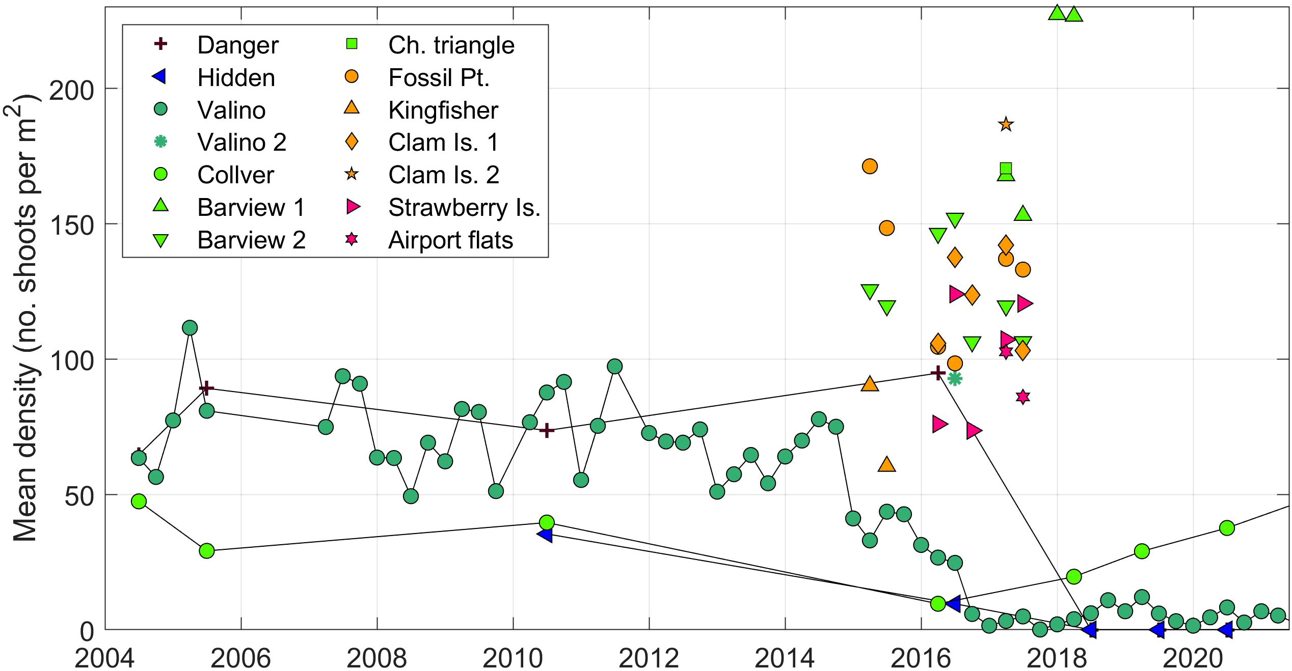
Figure 9 Density of eelgrass (number of shoots m²) until present for all eelgrass measurements from stations shown in Figure 2B and Supplemental Figure 1B. Stations are colored by general areas: purple to green = South Slough, yellow to pink = main channel. Connected symbols correspond to the stations shown in Figure 3A.

During 2013–2014, Z. marina phenology at Valino Island followed the expected seasonal pattern (Figure 3A): low percent cover and density in the winter months, with density of 54 shoots per m² during the Nov-2013 survey. In summer 2014, high productivity was registered at Valino Island, with a value of 78 shoots per m². By Apr-2015, however, eelgrass density decreased to significantly lower than the long-term mean (33 shoots per m²), after the warming of estuarine waters during the previous fall and winter (Figure 6). Beyond the seasonal high of Jul-2015 (44 shoots per m²), density remained very low with values around 5 shoots per m² through to present day. This decay was not only observed in the density, but in the height of the canopy and the total percent cover. The other eelgrass survey sites at Collver Point, Danger Point, and Hidden Creek, also show low density, canopy height, number of flowering shoots and percent cover in the annual survey during this period (June-July 2016). Of these stations, only Collver, the most marine station, seems to recover with densities of 20 shoots per m² (Jun-2021). Surveys from stations outside of South Slough, show a small decrease yet not as large in magnitude or as long-lasting as at Valino Island, where a decay from 170 to 90 eelgrass shoots per m² was observed from Feb-2015 to Jul-2016 (Figure 9).

Discussion

Water quality, river discharge, air temperature, and wind stress data all demonstrate the strong seasonality in the Coos Estuary that mimics the larger scale CCS patterns (Figure 3). Warmer, saltier estuarine characteristics are observed between April and June, after which upwelling-favorable conditions produce cold, saltier waters at the ocean boundary, which finally transition to rainy, fresher and colder conditions in the estuary due to increased precipitation and reduced solar input. This seasonality is affected by interannual variations of the surrounding atmosphere and ocean, which modulate the estuary on all its boundaries, i.e., from the ambient ocean waters at its mouth, the river discharge input, and the atmospheric heat fluxes on its surface. However, the results do indicate that there is significant spatial variability in how the estuary responds to these larger-scale interannual variations due to local bathymetry and geometry constraints. For example, during the warmer years of 2014-2016, the up-estuary stations in South Slough (Valino, Winchester) are relatively warmer for extended periods of time compared to stations that are further away from the mouth in the main channel (e.g., BLM, KoKwel). This disparate response to environmental forcing may stress species, such as eelgrass, which occupy distinct regions of the estuary. By disentangling the impact of the temporal variations in estuarine water forcing with spatial factors (e.g., depth and distance from the mouth), we provide a framework to discuss how changing estuarine conditions might stress organisms differentially. We start by 1) examining changes outside the estuary at the basin scale, then move into 2) along-estuary gradients and spatial variability in hydrographic conditions before considering 3) long-term temporal variability due to the expected future warming under anthropogenic climate change. Finally, we examine the dramatic eelgrass decrease observed within the Coos Estuary in the context of the temperature variability described above.

Basin scale variability

Though many organisms grow in wide temperature ranges, a persistent anomaly may stress species such as eelgrass beyond recovery (e.g., >1.5 °C above normal, Table 2). During the winter of 2013–2014, the PNW experienced drought conditions, related to a persistent atmospheric high-pressure ridge linked to variability in the North Pacific Oscillation (Figure 1), a known precursor of El Niño conditions (Wang et al., 2014; Di Lorenzo and Mantua, 2016). The high-pressure also affected the arrival of winter storms in the PNW, resulting in the below-average water-year cumulative discharge in the Coos River (Figure 4D) and increased air temperature in the Coos Estuary in 2013-2014 (Figure 4C). This combination produced anomalously warm water temperatures during 2014 in the Coos Estuary. During the winter of 2013, the “Blob” was observed in the North Pacific and moved onto the shelf from Sep-2014 until Mar-2015, increasing SST more than 1.5 °C eelgrass threshold at the Stonewall buoy. Positive anomalies (>1.5°C, Figure 1B) were observed at Stonewall again from Jul-2015 to May-2016 related to a second marine heatwave (Di Lorenzo and Mantua, 2016). During the El Niño event in 2015 SST anomalies of 4 °C where registered at the Stonewall buoy, with maximum anomalies between Nov-2015 and Jan-2016. This El Niño event increased the likelihood of storms and precipitation in the PNW, increasing river discharge at the Coos River, as registered during 2015-2016 (Alexander et al., 2002; Goodman et al., 2018). This atmospheric connection also reduces upwelling-favorable winds which would normally bring colder waters during the late summer to the Coos Estuary (Capotondi et al., 2019).

Though the El Niño conditions can have a strong impact on the PNW, observational and modelling efforts (Jacox et al., 2016) indicate that the temperature anomalies observed on the continental shelf (Figure 1B) were mostly related to the marine heatwave. At the Stonewall buoy, the combination of these basin-scale processes increased water temperature (>1.5°C warmer than the 2004-2014 climatology) during the fall and winter of 2014, 2015 and slightly during 2016 (Figure 4B). The warm anomalies slightly decreased during the upwelling seasons of each year but picked up again after the winds started to relax (Figure 4A). These anomalies were observed in estuaries from San Francisco Bay (up to 3°C, Cloern et al., 2017), to Puget Sound (up to 1 °C, Jackson et al., 2018). In the Coos Estuary, anomalies up to 2°C were observed in Charleston, 3 km from the mouth, in March-2015. Increased water temperature at the ocean boundary will increase the heat that can be advected into the estuary and alter the along-estuary temperature gradient.

Along-estuary differences in temperature

Water temperature and salinity levels in estuaries are controlled by the interaction of advective fluxes, atmospheric fluxes and exchanges with the ocean boundary at the estuary mouth and the river boundaries at each freshwater input (Smith, 1983; Stevenson and Niiler, 1983). Our subtidal data highlights the influence of the ocean end-member on temperature in the estuary, which weakens with distance from the mouth due to the impact of the river end-member. Additionally, the along and across-estuary temperature gradients vary with depth, which is set by dredging in the Coos and many other estuaries of the PNW, though not within South Slough (Eidam et al., 2020). Though tidal advection is a major factor in the Coos Estuary (Conroy et al., 2020), South Slough shows greater temporal temperature variability than the main channel, most likely due to a combination of shallower channels (~5 m) and increased areas of tidal flats (Sutherland and O’Neill, 2016). Dynamically, the main channel stations are located farther seaward than the up-estuary stations in South Slough, even though their physical distances are closer. That is, if one accounts for the length of the salinity intrusion over the main channel versus South Slough, the Valino and Winchester stations would be located up-estuary of any existing observation’s locations in the main channel. As temperature increases beyond the climatology due to interannual or climate variability, the storage and flux of heat will change and affect the estuarine ecosystems.

Our qualitative approach to the heat budget in the Coos Estuary (Eq. 1) allows one to spatially and temporally fingerprint the anomalously warm water due to interannual variability during 2014-2016, and can be applied to other estuaries in the PNW (Figure 1A). The analysis for the Coos Estuary highlights the increased atmospheric heat flux in South Slough during the marine heatwave in 2014-2015, due to the inverse dependence on depth.

On top of the anomalous atmospheric heat flux during 2014–2016, the advective heat flux shows changes due to variability of the along-estuary temperature gradient as well as changes to along-estuary velocity. Our data shows that during the dry seasons of 2014–2016 (Figure 8D), the temperature gradient was stronger (more negative, especially in 2015–2016), due to warmer waters in the oceanic end member (Charleston – red bars in Figure 8). During drought years, a decreased estuarine circulation could potentially increase temperature inside the estuary. During normal river discharge years, the ocean influx is greater, so if these ocean waters are relatively warm that could also lead to an increase in temperature within the estuary. As ocean temperature increased in late 2014 on the ocean-end member, an anomalous temperature gradient is observed in South Slough (Figure 8), when Winchester Creek temperature increases (Figure 6). In 2015-2016 the water-year cumulative discharge was normal. A simple back-of-the-envelope calculation of the second term in Eq. 1 using $\frac{\partial T_{av}}{\partial x}$ requires speeds of 0.01 m s^-1 in South Slough. This speed can be estimated from observations by dividing the river discharge by the estuarine cross-sectional area of interest. We use available data from water-penetrating airborne lidar survey (Conroy et al., 2020), to calculate the area for a cross section near Valino, and a scaled river discharge for the watershed area in Winchester, Joe Ney Creek, Elliot Creek and John B. Creek (Figure 2). This produces maximum speeds of 0.014 m s^-1 in the winter, confirming our advective flux calculations.

Long term variability

The combination of anomalously warm water in the PNW with anomalously warm air temperature and advection of riverine waters, produced anomalously warm estuarine waters in South Slough during 2014–2016. These potentially stressful years motivate the question if we can expect this combination to occur more or less often in a warming climate. Observations along the PNW coast (including the ones presented here) show responses related to the large-scale climatic patterns (e.g., ENSO, PDO and NPGO), where positive basin-scale temperature anomalies led to increased temperature inside estuarine systems (Johnson et al., 2003; Cloern et al., 2017; Jackson et al., 2018). Climate model simulations suggest that in the future, an increased variance of the North Pacific Oscillation (NPO) can be expected (Wang et al., 2014; Black et al., 2018; Capotondi et al., 2019), which was the leading cause of the marine heatwave (the Blob) and also connected to the 2013-2014 drought conditions in the PNW. El Niño events, correlated to higher temperature and sea level in the PNW are also expected to occur more often in the future (Wang et al., 2014; Di Lorenzo and Mantua, 2016). El Niño events have also been correlated to a more intense downwelling and later onset of summer upwelling in the PNW both of which would produce warmer temperatures in the ocean end-member (Frischknecht et al., 2015). Additionally, it is still unclear whether river discharge will increase or decrease with climate change in the PNW, most models agree that in South Slough, Yaquina, Willapa and Coquille estuary, higher discharge is expected in October and November, while lower discharge is expected in July and August (Steele et al., 2012), moving the dry period in these estuaries earlier in the year, similar to that observed in 2014–2016.

The temperature time series here, focused on the last decade, can hint at what can be expected in the future. Traditionally, the spring and fall transitions that mark the beginning and end of upwelling season, respectively, also demarcate the arrival of distinct transport pathways across the shelf, enhanced primary and secondary production, and many other ecological processes. These transitions have been changing in time over the past century, in response to the ocean, river and atmospheric forcing dictated to some degree by basin-scale processes and climate change (Di Lorenzo et al., 2015; Black et al., 2018; Capotondi et al., 2019). Given the importance of the estuarine temperature gradient to the ecological health of South Slough and other PNW estuaries, we develop a method similar to the upwelling index produced by Pierce et al. (2006). That is, we find the day of the year when the landward and shallowest station is warmer than the most marine-influenced station (here that means the Winchester to Charleston temperature gradient in summer) and the day of the year in which this relationship reverses (Winchester is colder than Charleston in winter, Figure 10A). Figure 10B shows these “transition” days for all the years available, as well as the Spring/Fall transition from Pierce et al. (2006), calculated using daily upwelling indices, proportional to alongshore wind stress at 45^oN. This transition from spring to fall index at 45°N shows a progression towards earlier upwelling, leading to a stronger influence of the ocean in PNW estuaries (Pierce et al., 2006). Due to the dependence of the temperature gradient on discharge, we also define transition dates for the Coos Estuary River discharge as greater and smaller than 3.2 m³ s^-1 (average during dry season). Our 14-year-long time series shows a similar pattern to the Spring Transition dates that mark the beginning of upwelling season (r² = 0.56), while the Fall transition is delayed by 23 days in average (r² = 0.54). Our data also show that the end of the warming period in South Slough does not only depend on the oceanic conditions (which is correlated with the Pierce index), but also on river discharge (r² = 0.47) and atmospheric forcing (r² = 0.57). Hence, in a future of warming climate, when large-scale oscillations are expected to occur more frequently (Di Lorenzo and Mantua, 2016), an increase in the temperature in the estuaries of the PNW, as well as an extended dry, warm season can be expected, which will have large impacts on these ecosystems.

FIGURE 10

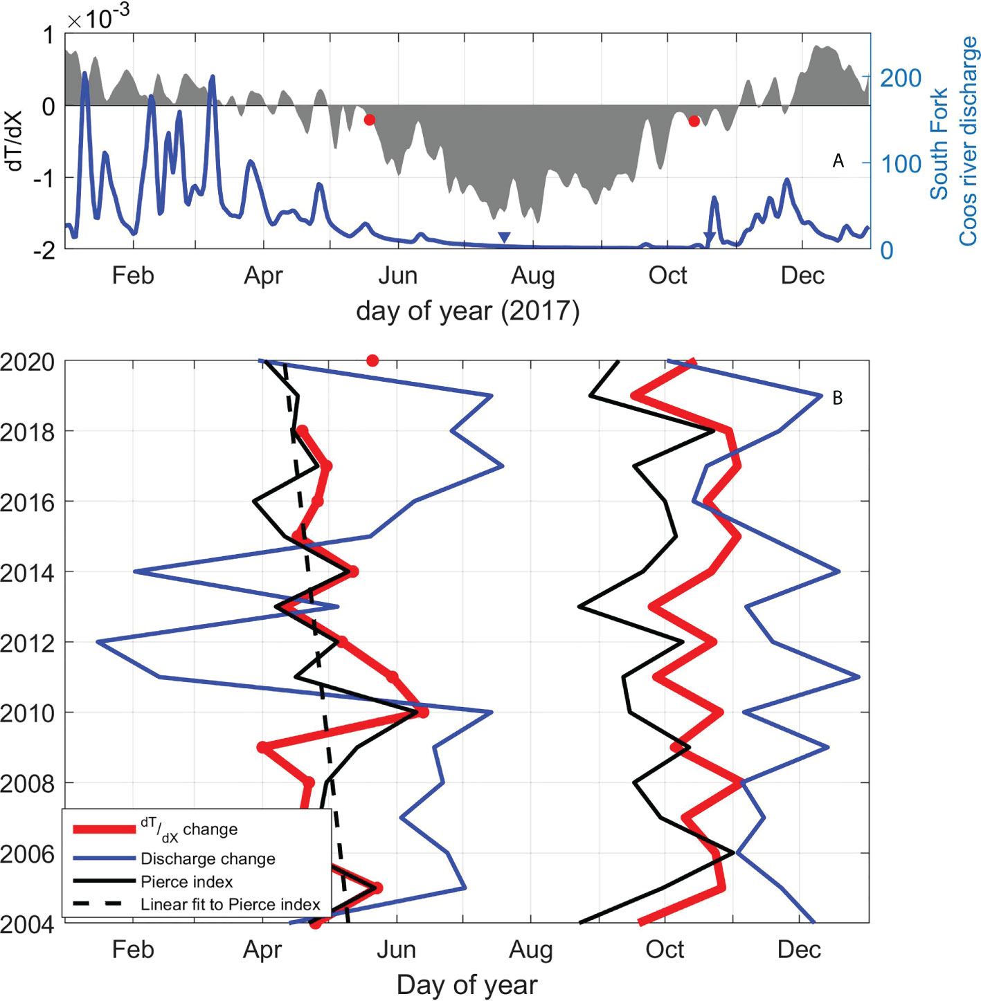
Figure 10 (A) Temperature gradient and discharge transition date determination example (2017) and zero-crossing of gradients before and after the dry season. (B) Annual variability of transition periods: in red spring and summer temperature gradient change (notice no available data for 2019); in blue South Fork of the Coos River discharge transition dates; in black Pierce index (2006) spring and fall transition dates for all years. Statistically significant linear fit to Pierce index spring transition (2006) in black broken line.

Increased estuary temperature due to climate variability is widely documented (Nixon et al., 2004; Preston, 2004; Seekell and Pace, 2011), yet the combination of intensified end-member heat sources and their impact on the hydrodynamics is not as well described. Our transition-day time series, though short and not statistically significant ($\frac{\partial T_{av}}{\partial x}$ slope ≠ 0, r² = 0.03), is significantly correlated to the Pierce transition index (r² = 0.55), which extends from 1995 to 2020. The Summer Pierce transition index (and by correlation, our estuarine temperature gradient) shows a shift towards an earlier beginning of the summer, and later start of the winter season (Summer transition date slope ≠ 0, r² = 0.3), as also predicted from river discharge forecasting (Steele et al., 2012). This extended earlier dry season can affect the ecosystem by changing ranges of temperature, stratification, and may produce hypoxia (Officer et al., 1984) or affect organisms such as eelgrass and oysters (Borde et al., 2003; Thom et al., 2003; Black et al., 2014). Finally, as temperature increases, the dynamic influence on water density may become significant, especially during the summer, affecting the baroclinic circulation in estuaries, by intensifying or weakening the along-channel density differences that drive estuarine circulation (Hickey et al., 2003; Raimonet and Cloern, 2017).

Effects on eelgrass (Zostera marina)

In-situ observations as well as remotely sensed surveys reveal that eelgrass has decreased in abundance in the up-estuary portions of South Slough and the greater Coos Estuary (Figure 2; Supplementary Figure 1). Remotely sensed data from 2005 and 2016 show a decrease of eelgrass-covered area in the Coos Estuary, with higher survival in the main channel than in South Slough (Supplementary Figure 2B), despite the proximity of the sub-estuary to the mouth of the estuary and influence of coastal waters (Raimonet and Cloern, 2017; Magel et al., 2022). Notably, stations in South Slough that were only 3-10 km from the mouth are less marine-influenced than the main channel stations that reside 5-15 km from the mouth, a result that is consistent with the structure of the salinity intrusion in the Coos Estuary (Conroy et al., 2020). Though our data show increased water and air temperature over the whole estuary (Figure 6), a stronger decline of eelgrass was also registered in in-situ stations within the up-estuary portion of South Slough (Figure 3).

Eelgrass is sensitive to temperature stress, as it can increase photosynthetic and respiration rates (Beca-Carretero et al., 2018), and lead to higher susceptibility to wasting disease (Kaldy, 2014). Our results suggest that the MHWs and increased air temperature contributed to the eelgrass density decline in 2015 (Figures 3, 10, Supplementary Figure 4). In contrast, Magel et al. (2022) show an increase in eelgrass at one annually-surveyed station (Barview, see Figure 9) closer to the main channel than Valino Island. Their results show an increase in eelgrass density and biomass during the summer of 2015 and summer of 2016, followed by a decline to longer term average values. They attribute the anomalous increase during a MHW to increased upwelling. However, the annual frequency of those surveys leaves open questions about lags in response, as well as the co-occurrence of other biological interactions (epiphyte and macroalgae interaction). Our data shows that despite the short seasonal increase in eelgrass cover, the density of eelgrass at Valino Island declined again in 2016 when anomalously warm waters related to the El Niño event were again observed. Eelgrass at Valino has not fully recovered since (Figure 3). Stronger declines in eelgrass density were registered in the stations in South Slough compared to stations in the main channel (Supplementary Figure 2C) which are warmer for extended periods of time, especially during 2014-2016 (Supplementary Figure 3). This temperature anomaly can be attributed not only to the distance from the oceanic end-member and the river end-member, but also to storage of heat in shallower areas, such as those where eelgrass is found (0.5–1.0 m MLLW).

Conclusions

In the Pacific Northwest, long-term and large spatial-scale processes, such as El Niño and marine heatwaves, imprint interannual variability on top of typical seasonal trends. Here we used 14 years of data from the Coos Estuary, in southwestern Oregon, to quantify the effects of anomalous oceanic and atmospheric conditions on the estuary, which includes a dramatic die-off in eelgrass.

Superimposed on the interannual and long-term trends, PNW estuaries have a strong seasonal variability in temperature, in which lower water temperatures occur between November and March due to increased river discharge and wintertime atmospheric heat loss, producing a negative along-estuary temperature gradient. During the dry season, warmer air temperature and reduced river discharge increase water temperature, increasing the along-estuary temperature gradient. Between July and October, equatorward winds at the coast produce the upwelling of cold, saline, nutrient rich waters, increasing the temperature gradient further.

The combination of drought in 2013–2014, El Niño in 2014, the Blob marine heatwave in 2014–2015, and El Niño in 2016, produced anomalously warm waters in the coastal ocean outside of the estuary, along with warmer air temperatures and increased river discharge during the El Niño events. Inside the estuary, the warming was recorded in all the available water quality observations, with higher anomalies found in the shallower locations and those located further away from the estuary mouth. Water temperature increased landward, suggesting that river input and atmospheric heat flux may be important contributors to the anomalous conditions observed. These relatively higher temperatures found landward changed the overall along-estuary temperature gradient in the estuary with higher values in the beginning of the dry season before upwelling at the coast begins. Enhanced temperature gradients, along with relatively higher absolute temperatures in the upper estuary can cause stress on organisms, such as eelgrass, potentially explaining at least part of the die-off observed.

These temperature-related stress factors can be expected to occur more frequently in a warming climate, when more marine heatwaves and El Niño events can be expected. Our analysis shows that the temperature gradient in the Coos Estuary is correlated to an upwelling index that is proportional to alongshore wind stress. The longer upwelling index timeseries shows a shift towards earlier spring transitions, which would produce a longer summer season and possibly stronger influence of temperature on the baroclinic component of circulation.

Though time series available in the PNW are relatively short to assess long-term trends statistically, the observations analyzed here show 1) a shift to a later, shorter rainy season and 2) an increased synchrony of decadal (i.e., PDO) and interannual (i.e., MHWs) processes. As global temperatures warm due to climate change, we can expect an increased number of marine heatwaves and El Niño events, which will increase the temperature in Pacific Northwest estuaries, leading to changes in seasonal timing and potentially shifting the habitat areas in estuary ecosystems.

Data availability statement

The datasets presented in this study can be found in online repositories. The names of the repository/repositories and accession number(s) can be found below: http://nvs.nanoos.org https://www.ndbc.noaa.gov/station_page.php?station=46050, http://streamdata.cooswatershed.org/.

Author contributions

MJMJ is the lead author on the manuscript, developing the methodology, analyzing the observational data, and writing the manuscript. DS served as advisor, aiding in data interpretation and manuscript editing. AH collected and analyzed the eelgrass data, and aided in the results and discussion. All authors contributed to the article and approved the submitted version.

Funding

The Science Collaborative is funded by the National Oceanic and Atmospheric Administration and managed by the University of Michigan Water Center (NA19NOS4190058 and NA19NOS4200076). Additional funding for MJMJ was provided through Operations Award as 315-10 Davidson Fellowship and Student Development Opportunities. Funds for publication were granted through the Open Access Article Processing Charge Committee and the University of Oregon Libraries.

Acknowledgments

Eelgrass density data in locations outside of South Slough were obtained through several collaborations of SSNERR with the Oregon Department of Fish and Wildlife (ODFW SEACOR), Oregon State University (OSU) and the Pacific Marine Environmental Laboratory. This work was sponsored by the National Estuarine Research Reserve System Science Collaborative, which supports collaborative research that addresses coastal management problems important to the reserves.

Conflict of interest

The authors declare that the research was conducted in the absence of any commercial or financial relationships that could be construed as a potential conflict of interest.

Publisher’s note

All claims expressed in this article are solely those of the authors and do not necessarily represent those of their affiliated organizations, or those of the publisher, the editors and the reviewers. Any product that may be evaluated in this article, or claim that may be made by its manufacturer, is not guaranteed or endorsed by the publisher.

Supplementary material

The Supplementary Material for this article can be found online at: https://www.frontiersin.org/articles/10.3389/fmars.2022.930440/full#supplementary-material

References

Alexander M. A., Bladé I., Newman M., Lanzante J. R., Lau N.-C., Scott J. D. (2002). The atmospheric bridge: The influence of ENSO teleconnections on air–Sea interaction over the global oceans. J. Clim. 15, 2205–2231. doi: 10.1175/1520-0442(2002)015<2205:TABTIO>2.0.CO;2

CrossRef Full Text | Google Scholar

Baptista A. M. (1989). Salinity in coos bay (Oregon: U.S. Army Engineer District).

Google Scholar

Barnard P. L., Hoover D., Hubbard D. M., Snyder A., Ludka B. C., Allan J., et al. (2017). Extreme oceanographic forcing and coastal response due to the 2015-2016 El niño. Nat. Commun. 8, 6–13. doi: 10.1038/ncomms14365

PubMed Abstract | CrossRef Full Text | Google Scholar

Basilio A., Searcy S., Thompson A. R. (2017). Effects of the blob on settlement of spotted sand bass, paralabrax maculatofasciatus, to mission bay, San Diego, CA. PloS One 12, 6–8. doi: 10.1371/journal.pone.0188449

CrossRef Full Text | Google Scholar

Beca-Carretero P., Olesen B., Marbà N., Krause-Jensen D. (2018). Response to experimental warming in northern eelgrass populations: Comparison across a range of temperature adaptations. Mar. Ecol. Prog. Ser. 589, 59–72. doi: 10.3354/meps12439

CrossRef Full Text | Google Scholar

Bi H., Peterson W. T., Strub P. T. (2011). Transport and coastal zooplankton communities in the northern California current system. Geophys. Res. Lett. 38, 1–5. doi: 10.1029/2011GL047927

CrossRef Full Text | Google Scholar

Black B. A., Sydeman W. J., Frank D. C., Griffin D., Stahle D. W., Garcia-Reyes M., et al. (2014). Six centuries of variability and extremes in a coupled marine-terrestrial ecosystem. Science 345, 1498–1502. doi: 10.1126/science.1253209

PubMed Abstract | CrossRef Full Text | Google Scholar

Black B. A., van der Sleen P., Di Lorenzo E., Griffin D., Sydeman W. J., Dunham J. B., et al. (2018). Rising synchrony controls western north American ecosystems. Glob. Change Biol. 24, 2305–2314. doi: 10.1111/gcb.14128

CrossRef Full Text | Google Scholar

Bond N. A., Cronin M. F., Freeland H., Mantua N. (2015). Causes and impacts of the 2014 warm anomaly in the NE pacific. Geophys. Res. Lett. 42, 3414–3420. doi: 10.1002/2015GL063306

CrossRef Full Text | Google Scholar

Borde A. B., Thom R. M., Rumrill S., Miller L. M. (2003). Geospatial habitat change analysis in pacific Northwest coastal estuaries. Estuaries 26, 1104–1116. doi: 10.1007/bf02803367

CrossRef Full Text | Google Scholar

Capotondi A., Sardeshmukh P. D., Di Lorenzo E., Subramanian A. C., Miller A. J. (2019). Predictability of US West coast ocean temperatures is not solely due to ENSO. Sci. Rep. 9, 1–10. doi: 10.1038/s41598-019-47400-4

PubMed Abstract | CrossRef Full Text | Google Scholar

Chhak K., Di Lorenzo E. (2007). Decadal variations in the California current upwelling cells. Geophys. Res. Lett. 34, 1–6. doi: 10.1029/2007GL030203

CrossRef Full Text | Google Scholar

Clinton P. J., Young D. R., Specht D. T., Lee I. I. ,. H. (2007). A guide to mapping intertidal eelgrass and nonvegetated habitats in estuaries of the pacific Northwest USA (National Health and Environmental Effects Research Laboratory ( NHEERL ) Office of Research and D. Newport OR. by Project Officer: Walter G . Nelson.

Google Scholar

Cloern J. E., Jassby A. D., Schraga T. S., Nejad E., Martin C. (2017). Ecosystem variability along the estuarine salinity gradient: Examples from long-term study of San Francisco bay. Limnol. Oceanogr. S272–S291. doi: 10.1002/lno.10537

CrossRef Full Text | Google Scholar

Conroy T., Sutherland D. A., Ralston D. K. (2020). Estuarine exchange flow variability in a seasonal, segmented estuary. J. Phys. Oceanogr. 50, 595–613. doi: 10.1175/JPO-D-19-0108.1

CrossRef Full Text | Google Scholar

Costanza R., D’Arge R., de Groot R., Farber S., Grasso M., Hannon B., et al. (1997). The value of the world’s ecosystem services and natural capital. Nature 387, 253–260. doi: 10.1038/387253a0

CrossRef Full Text | Google Scholar

Daly E. A., Brodeur R. D., Auth T. D. (2017). Anomalous ocean conditions in 2015: Impacts on spring Chinook salmon and their prey field. Mar. Ecol. Prog. Ser. 566, 168–182. doi: 10.3354/meps12021

CrossRef Full Text | Google Scholar

Davis K. A., Banas N. S., Giddings S. N., Siedlecki S. A., MacCready P., Lessard E. J., et al. (2014). Estuary-enhanced upwelling of marine nutrients fuels coastal productivity in the U.S. pacific Northwest. J. Geophys. Res. Ocean. 119 (12), 8778–8799. doi: 10.1002/2014JC010248

CrossRef Full Text | Google Scholar

Delefosse M., Povidisa K., Poncet D., Kristensen E., Olesen B. (2016). Variation in size and chemical composition of seeds from the seagrass Zostera marina-ecological implications. Aquat. Bot. 131, 7–14. doi: 10.1016/j.aquabot.2016.02.003

CrossRef Full Text | Google Scholar

Di Lorenzo E., Fiechter J., Schneider N., Braceo A., Miller A. J., Franks P. J. S., et al. (2009). Nutrient and salinity decadal variations in the central and eastern north pacific. Geophys. Res. Lett. 36, 2003–2008. doi: 10.1029/2009GL038261

CrossRef Full Text | Google Scholar

Di Lorenzo E., Liguori G., Schneider N., Furtado J. C., Anderson B. T., Alexander M. A. (2015). ENSO and meridional modes: A null hypothesis for pacific climate variability. Geophys. Res. Lett. 42, 9440–9448. doi: 10.1002/2015GL066281

CrossRef Full Text | Google Scholar

Di Lorenzo E., Mantua N. (2016). Multi-year persistence of the 2014/15 north pacific marine heatwave. Nat. Clim. Change 6, 1042–1047. doi: 10.1038/nclimate3082

CrossRef Full Text | Google Scholar

Di Lorenzo E., Schneider N., Cobb K. M., Franks P. J. S., Chhak K., Miller A. J., et al. (2008). North pacific gyre oscillation links ocean climate and ecosystem change. Geophys. Res. Lett. 35, 2–7. doi: 10.1029/2007GL032838

CrossRef Full Text | Google Scholar

Echavarria-Heras H. A., Solana-Arellano E., Franco-Vizcaíno E. (2006). The role of increased Sea surface temperature on eelgrass leaf dynamics: Onset of El niño as a proxy for global climate change in San quintín bay, Baja California. Bull. South. Calif. Acad. Sci. 105, 113–127. doi: 10.3160/0038-3872(2006)105[113:TROISS]2.0.CO;2

CrossRef Full Text | Google Scholar

Eidam E. F., Sutherland D. A. A., Ralston D. K. K., Dye B., Conroy T., Schmitt J., et al. (2020). Impacts of 150 years of shoreline and bathymetric change in the coos estuary, Oregon, USA. Estuaries Coasts 1170–1188. doi: 10.1007/s12237-020-00732-1

CrossRef Full Text | Google Scholar

Emmett R., Llansó R., Newton J., Thom R. M., Hornberger M., Morgan C., et al. (2000). Geographic signatures of north American West coast estuaries. Estuaries 23, 765. doi: 10.2307/1352998

CrossRef Full Text | Google Scholar

Evans E. C., McGregor G. R., Petts G. E. (1998). River energy budgets with special reference to river bed processes. Hydrol. Process. 12, 575–595. doi: 10.1002/(SICI)1099-1085(19980330)12:4<575::AID-HYP595>3.0.CO;2-Y

CrossRef Full Text | Google Scholar

Frischknecht M., Münnich M., Gruber N. (2015). Remote versus local influence of ENSO on the California current system. J. Geophys. Res. Ocean. 120, 1353–1374. doi: 10.1002/2014JC010531

CrossRef Full Text | Google Scholar

Gao Y., Fang J., Du M., Fang J., Jiang W., Jiang Z. (2017). Response of the eelgrass (Zostera marina l.) to the combined effects of high temperatures and the herbicide, atrazine. Aquat. Bot. 142, 41–47. doi: 10.1016/j.aquabot.2017.06.005

CrossRef Full Text | Google Scholar

Gentemann C. L., Fewings M. R., García-Reyes M. (2017). Satellite sea surface temperatures along the West coast of the united states during the 2014–2016 northeast pacific marine heat wave. Geophys. Res. Lett. 44, 312–319. doi: 10.1002/2016GL071039

CrossRef Full Text | Google Scholar

Goodman A. C., Thorne K. M., Buffington K. J., Freeman C. M., Janousek C. N. (2018). El Niño increases high-tide flooding in tidal wetlands along the U.S. pacific coast. J. Geophys. Res. Biogeosciences 123, 3162–3177. doi: 10.1029/2018JG004677

CrossRef Full Text | Google Scholar

Groner M., Eisenlord M., Yoshioka R., Fiorenza E., Dawkins P., Graham O., et al. (2021). Warming sea surface temperatures fuel summer epidemics of eelgrass wasting disease. Mar. Ecol. Prog. Ser. 679, 47–58. doi: 10.3354/meps13902

CrossRef Full Text | Google Scholar

Groth S., Rumrill S. (2009). History of Olympia oysters ( ostrea lurida carpenter 1864) in Oregon estuaries, and a description of recovering populations in coos bay. J. Shellfish Res. 28, 51–58. doi: 10.2983/035.028.0111

CrossRef Full Text | Google Scholar

Hessing-Lewis M. L., Hacker S. D., Menge B. A., Rumrill S. S. (2011). Context-dependent eelgrass-macroalgae interactions along an estuarine gradient in the pacific Northwest, USA. Estuaries Coasts 34, 1169–1181. doi: 10.1007/s12237-011-9412-8

CrossRef Full Text | Google Scholar

Hickey B. M., Banas N. S. (2003). Oceanography of the U. S. doi: 10.1007/bf02803360

CrossRef Full Text | Google Scholar

Hickey B. M., Zhang X., Banas N. S. (2003). Coupling between the California current system and a coastal plain estuary in low riverflow conditions. J. Geophys. Res. 108, 1–20. doi: 10.1029/2002JC001737

CrossRef Full Text | Google Scholar

Hosack G. R., Dumbauld B. R., Ruesink J. L., Armstrong D. A. (2006). Habitat associations of estuarine species: Comparisons of intertidal mudflat, seagrass (Zostera marina), and oyster (Crassostrea gigas) habitats. Estuaries Coasts 29, 1150–1160. doi: 10.1007/BF02781816

CrossRef Full Text | Google Scholar

Huyer A. (1983). Coastal upwelling in the California current system. Prog. Oceanogr. 12, 259–284. doi: 10.1016/0079-6611(83)90010-1

CrossRef Full Text | Google Scholar

Huyer A., Smith R. L., Fleischbein J. (2002). The coastal ocean off Oregon and northern California during the 1997-8 El niño. Prog. Oceanogr. 54, 311–341. doi: 10.1016/S0079-6611(02)00056-3

CrossRef Full Text | Google Scholar

Huyer A., Wheeler P. A., Strub P. T., Smith R. L., Letelier R., Kosro P. M. (2007). Progress in oceanography the Newport line off Oregon – studies in the north East pacific 75 (2), 126–160. doi: 10.1016/j.pocean.2007.08.003

CrossRef Full Text | Google Scholar

Jackson J. M., Johnson G. C., Dosser H. V., Ross T. (2018). Warming from recent marine heatwave lingers in deep British Columbia fjord. Geophys. Res. Lett. 45, 9757–9764. doi: 10.1029/2018GL078971

CrossRef Full Text | Google Scholar

Jacox M. G., Hazen E. L., Zaba K. D., Rudnick D. L., Edwards C. A., Moore A. M., et al. (2016). Impacts of the 2015–2016 El niño on the California current system: Early assessment and comparison to past events. Geophys. Res. Lett. 43, 7072–7080. doi: 10.1002/2016GL069716

CrossRef Full Text | Google Scholar

Jarvis J. C., Moore K. A., Kenworthy W. J. (2012). Characterization and ecological implication of eelgrass life history strategies near the species’ southern limit in the western north Atlantic. Mar. Ecol. Prog. Ser. 444, 43–56. doi: 10.3354/meps09428

CrossRef Full Text | Google Scholar

Johnson M. R., Williams S. L., Lieberman C. H., Solbak A. (2003). Changes in the abundance of the seagrasses Zostera marina l. (eelgrass) and ruppia maritima l. (widgeongrass) in San Diego, California, following an El niño event. Estuaries 26, 106–115. doi: 10.1007/BF02691698

CrossRef Full Text | Google Scholar

Kaldy J. (2012). Influence of light, temperature and salinity on dissolved organic carbon exudation rates in Zostera marina l. Aquat. Biosyst. 8, 1–12. doi: 10.1186/2046-9063-8-19

PubMed Abstract | CrossRef Full Text | Google Scholar

Kaldy J. E. (2014). Effect of temperature and nutrient manipulations on eelgrass Zostera marina l. from the pacific Northwest, USA. J. Exp. Mar. Bio. Ecol. 453, 108–115. doi: 10.1016/j.jembe.2013.12.020

CrossRef Full Text | Google Scholar

Kalnay E., Kanamitsu M., Kistler R., Collins W., Deaven D., Gandin L., et al. (1996). The NCEP/NCAR 40-year reanalysis project. Bull. Am. Meteorol. Soc 77, 437–471. doi: 10.1175/1520-0477(1996)077<0437:TNYRP>2.0.CO;2

CrossRef Full Text | Google Scholar

Large W. G., Pond S. (1981). Open Ocean Momentum Flux Measurements in Moderate to Strong Winds. J. Phys. Oceanogr. 11, 324–336. doi: 10.1175/1520-0485(1981)011<0324.

CrossRef Full Text | Google Scholar

Lee H. II, Brown C. A. (eds.) (2009). Classification of Regional Patterns of Environmental Drivers And Benthic Habitats in Pacific Northwest Estuaries. U.S. EPA, Office of Research and Development, National Health and Environmental Effects Research Laboratory, Western Ecology Division.

Google Scholar

Lee K. S., Park S. R., Kim Y. K. (2007). Effects of irradiance, temperature, and nutrients on growth dynamics of seagrasses: A review. J. Exp. Mar. Bio. Ecol. 350, 144–175. doi: 10.1016/j.jembe.2007.06.016

CrossRef Full Text | Google Scholar

Logerwell E. A., Mantua N., Lawson P. W., Francis R. C., Agostini V. N. (2003). Tracking environmental processes in the coastal zone for understanding and predicting Oregon coho (Oncorhynchus kisutch) marine survival. Fish. Oceanogr. 12, 554–568. doi: 10.1046/j.1365-2419.2003.00238.x

CrossRef Full Text | Google Scholar

Magel C. L., Chan F., Hessing-Lewis M., Hacker S. D. (2022). Differential responses of eelgrass and macroalgae in pacific Northwest estuaries following an unprecedented NE pacific ocean marine heatwave. Front. Mar. Sci. 9. doi: 10.3389/fmars.2022.838967

PubMed Abstract | CrossRef Full Text | Google Scholar

McKay P., Iorio D. (2008). Heat budget for a shallow, sinuous salt marsh estuary. Cont. Shelf Res. 28, 1740–1753. doi: 10.1016/j.csr.2008.04.008

CrossRef Full Text | Google Scholar

Milcu A. I., Hanspach J., Abson D., Fischer J. (2013). Cultural ecosystem services: A literature review and prospects for future research. Ecol. Soc 18. doi: 10.5751/ES-05790-180344

CrossRef Full Text | Google Scholar

Miller J. A., Shanks A. L. (2004). Ocean-estuary coupling in the Oregon upwelling region: Abundance and transport of juvenile fish and of crab megalopae. Mar. Ecol. Prog. Ser. 271, 267–279. doi: 10.3354/meps271267

CrossRef Full Text | Google Scholar

Nejrup L. B., Pedersen M. F. (2008). Effects of salinity and water temperature on the ecological performance of Zostera marina. Aquat. Bot. 88, 239–246. doi: 10.1016/j.aquabot.2007.10.006

CrossRef Full Text | Google Scholar

Nixon S. W., Granger S., Buckley B. A., Lamont M., Rowell B. (2004). A one hundred and seventeen year coastal water temperature record from woods hole, Massachusetts. Estuaries 27, 397–404. doi: 10.1007/BF02803532

CrossRef Full Text | Google Scholar

NOAA National Estuarine Research Reserve System (NERRS) (2020) System-wide monitoring program (NOAA NERRS Cent. Data Manag. Off). Available at: http://www.nerrsdata.org (Accessed June 11, 2020).

Google Scholar

Officer C. B., Biggs R. B., Taft J. L., Cronin L. E., Tyler M. A., Boynton W. R. (1984). Chesapeake Bay anoxia: Origin, development, and significance. Science 223, 22–27. doi: 10.1126/science.223.4631.22

PubMed Abstract | CrossRef Full Text | Google Scholar

Peterson W. T., Fisher J. L., Strub P. T., Du X., Risien C., Peterson J., et al. (2017). The pelagic ecosystem in the northern California current off Oregon during the 2014-2016 warm anomalies within the context of the past 20 years. J. Geophys. Res. Ocean. 122, 7267–7290. doi: 10.1002/2017JC012952

CrossRef Full Text | Google Scholar

Phillips R. C. (1984). The ecology of eelgrass meadows in the pacific Northwest: a community profile. US Fish Wildl. Serv.

Google Scholar

Phillips R. C., McMillan C., Bridges K. W. (1983). Phenology of eelgrass, Zostera marina l., along latitudinal gradients in north America. Aquat. Bot. 15, 145–156. doi: 10.1016/0304-3770(83)90025-6

CrossRef Full Text | Google Scholar

Pierce S. D., Barth J. A., Thomas R. E., Fleischer G. W. (2006). Anomalously warm July 2005 in the northern California current: Historical context and the significance of cumulative wind stress. Geophys. Res. Lett. 33, 2–7. doi: 10.1029/2006GL027149

CrossRef Full Text | Google Scholar

Preston B. L. (2004). Observed winter warming of the Chesapeake bay estuary, (1949-2002): Implications for ecosystem management. Environ. Manage. 34, 125–139. doi: 10.1007/s00267-004-0159-x

PubMed Abstract | CrossRef Full Text | Google Scholar

Raimonet M., Cloern J. E. (2017). Estuary–ocean connectivity: fast physics, slow biology. Glob. Change Biol. 23, 2345–2357. doi: 10.1111/gcb.13546

CrossRef Full Text | Google Scholar

Roegner G. C., Hickey B. M., Newton J. A., Shanks A. L., Armstrong D. A. (2002). Wind-induced plume and bloom intrusions into willapa bay, Washington. Limnol. Oceanogr. 47, 1033–1042. doi: 10.4319/lo.2002.47.4.1033

CrossRef Full Text | Google Scholar

Roegner G. C., Needoba J. A., Baptista A. M. (2011). Coastal upwelling supplies oxygen-depleted water to the columbia river estuary. PloS One 6. doi: 10.1371/journal.pone.0018672

CrossRef Full Text | Google Scholar

Roegner G. C., Shanks A. L. (2001). Import of coastally-derived chlorophyll a to south Slough, Oregon. Estuaries 244, 244–256. doi: 10.2307/1352948

CrossRef Full Text | Google Scholar

Salo T., Pedersen M. F. (2014). Synergistic effects of altered salinity and temperature on estuarine eelgrass (Zostera marina) seedlings and clonal shoots. J. Exp. Mar. Bio. Ecol. 457, 143–150. doi: 10.1016/j.jembe.2014.04.008

CrossRef Full Text | Google Scholar

Schneider S. (1993). ““Scenarios of global warming,”,” in Biotic interactions and global change. Eds. Kareiva P., Kingsolver J., Huey R. (Sunderland, MA: Sinauer Associates), 9–23.

Google Scholar

Seekell D. A., Pace M. L. (2011). Climate change drives warming in the Hudson river estuary, new York (USA). J. Environ. Monit. 13, 2321–2327. doi: 10.1039/c1em10053j

PubMed Abstract | CrossRef Full Text | Google Scholar

Seppelt R., Dormann C. F., Eppink F. V., Lautenbach S., Schmidt S. (2011). A quantitative review of ecosystem service studies: Approaches, shortcomings and the road ahead. J. Appl. Ecol. 48, 630–636. doi: 10.1111/j.1365-2664.2010.01952.x

CrossRef Full Text | Google Scholar

Shanks A. L., Rasmuson L. K., Valley J. R., Jarvis M. A., Salant C., Sutherland D. A., et al. (2020). Marine heat waves, climate change, and failed spawning by coastal invertebrates. Limnol. Oceanogr. 65, 627–636. doi: 10.1002/lno.11331

CrossRef Full Text | Google Scholar

Sherman K., DeBruyckere L. A. (2018) Eelgrass habitats on the U.S. West coast. state of the knowledge of eelgrass ecosystem services and eelgrass extent. Available at: http://www.pacificfishhabitat.org/wp-content/uploads/2017/09/EelGrass_Report_Final_ForPrint_web.pdfeation%2020180109.pdf.

Google Scholar

Short F. T., Coles R. G. (2001). Global seagrass research methods. Eds. Short F. T., Coles R. G. (Elsevier: Amsterdam, The Netherlands).

Google Scholar

Short F. T., McKenzie L. J., Coles R. G., Vidler K. P., Gaeckle J. L. (2006). SeagrassNet Manual for Scientific Monitoring of Seagrass Habitat, Worldwide edition. University of New Hampshire Publication. 75

Google Scholar

Smith N. P. (1983). A comparison of winter and summer temperature variations in a shallow bar-built estuary. Estuaries 6, 2–9. doi: 10.2307/1351801

CrossRef Full Text | Google Scholar

Steele M. O., Chang H., Reusser D. A., Brown C. A., Jung I.-W. (2012). Potential climate-induced runoff changes and associated uncertainty in four Pacific Northwest estuaries: U.S. Geological Survey Open-File Report 2012-1274, 63. doi: 10.3133/ofr20121274

CrossRef Full Text | Google Scholar

Stevenson J. W., Niiler P. P. (1983). Upper ocean heat budget during the Hawaii-to-Tahiti shuttle experiment. J. Phys. Oceanogr. 13, 1894–1907. doi: 10.1175/1520-0485(1983)013<1894:UOHBDT>2.0.CO;2

CrossRef Full Text | Google Scholar

Strub P. T., Allen J. S., Huyer A., Smith R. L., Beardsley R. C. (1987). Seasonal cycles of currents, temperatures, winds, and sea level over the northeast pacific continental shelf: 35°N to 48°N. J. Geophys. Res. 92, 1507. doi: 10.1029/JC092iC02p01507

CrossRef Full Text | Google Scholar

Sutherland D. A., O’Neill M. A. (2016). Hydrographic and dissolved oxygen variability in a seasonal pacific Northwest estuary. Estuar. Coast. Shelf Sci. 172, 47–59. doi: 10.1016/j.ecss.2016.01.042

CrossRef Full Text | Google Scholar

Thom R. M., Albright R. G. (1990). Dynamics of benthic vegetation standing-stock, irradiance, and water properties in central Puget Sound. Mar. Biol. 104, 129–141. doi: 10.1007/BF01313166

CrossRef Full Text | Google Scholar

Thom R. M., Borde A. B., Rumrill S., Woodruff D. L., Williams G. D., Southard J. A., et al. (2003). Factors influencing spatial and annual variability in eelgrass (Zostera marina l.) meadows in willapa bay, Washington, and coos bay, Oregon, estuaries. Estuaries 26, 1117–1129. doi: 10.1007/BF02803368

CrossRef Full Text | Google Scholar

Thom R. M., Gaeckle J., Buenau K., Borde A., Vavrinec J., Aston L., et al. (2018). Eelgrass (Zostera marina L.) restoration in Puget Sound: development of a site suitability assessment process. Restor. Ecol. 26, 1066–1074. doi: 10.1111/rec.12702

PubMed Abstract | CrossRef Full Text | Google Scholar

Wang S.-Y., Hipps L., Gillies R. R., Yoon J.-H. (2014). Probable causes of the abnormal ridge accompanying the 2013-2014 California drought: ENSO precursor and anthropogenic warming footprint. Geophys. Res. Lett. 41, 3220–3226. doi: 10.1002/2014GL059748

CrossRef Full Text | Google Scholar

Wyrtki K. (1984). The slope of sea level along the equator during the 1982/1983 El nino. J. Geophys. Res. 89, 10419–10424. doi: 10.1029/JC089iC06p10419

CrossRef Full Text | Google Scholar

Zapata C., Puente A., Garca A., Garcia-Alba J., Espinoza J. (2018). Assessment of ecosystem services of an urbanized tropical estuary with a focus on habitats and scenarios. PloS One 13, 1–19. doi: 10.1371/journal.pone.0203927

CrossRef Full Text | Google Scholar

Zimmerman R. C., Smith R. D., Alberte R. S. (1989). Thermal acclimation and whole-plant carbon balance in Zostera marina L. (eelgrass). J. Exp. Mar. Bio. Ecol. 130, 93–109. doi: 10.1016/0022-0981(89)90197-4

CrossRef Full Text | Google Scholar