Assessing the patchiness of early life stage of a fish stock (Gadus morhua) and its contribution to the stock recruitment

Introduction

Patchiness or the variation in the local distribution of individuals in marine ecosystems may originate from both physical and biological properties of marine systems such as large physical phenomenon (e.g., oceanographic eddies, fronts, or filaments) and the capacity of organisms to aggregate together (e.g., schooling behavior or patchiness in mortality) (Trudnowska et al., 2016). The ecological importance of patches for marine individuals and population dynamics has been well known for several decades (McGurk, 1986; Kareiva, 1990). This type of spatial heterogeneous landscape has been described as the norm of ecosystems compared to a more homogeneous landscape (Grünbaum, 2012).

The heterogeneous landscape has implications for the fate of marine species. For example, small-scale patchiness can affect the predicted production on a larger scale compared to using mean field dynamics (Brentnall et al., 2003). Moreover, patchiness may influence species interactions (Genin, 2004) and potentially lead to altered buffering capacity against extreme events (e.g., storms and oil spills) (Lough et al., 1996; Langangen et al., 2017). The importance of patchiness and which physical scales are relevant to resolve species interactions that are affected by patchy distributions in the ecosystem is actively discussed in marine ecology (Fey and Szkudlarek-Pawełczyk, 2022).

In this study, we consider the example of the Northeast Arctic (NEA) stock of Atlantic cod (Gadus morhua). The species migrates annually from the feeding grounds in the Barents Sea to the spawning grounds along the coast of Norway. The offspring, in form of planktonic eggs and larvae, drift with the currents back to the nursery grounds in the Barents Sea (Bergstad et al., 1987). NEA cod is an important economic and human food resource. There has been a recent effort in understanding populations dynamics of fish in general and NEA cod in particular (Ottersen et al., 2014). Because the stock dynamics are dependent on the survival of the early life stages (ELS) for recruitment in the Barents Sea, it is important to elucidate the impact of patchy survival in these stages (Houde, 2008). Recently, modeling studies using particle tracking drift models have focused on the influence of spatial heterogeneous mortality of cod eggs and larvae, albeit limited by observational constraints and computational capacity to relatively large scales (Langangen et al., 2014; Langangen et al., 2016). However, it is still unclear whether mortality varies at smaller scales and the potential ecological importance of such variations. In a thought experiment, Langangen et al. (2017) illustrated how spatial variability in mortality may propagate from the cohort to the population level. Building on this experiment, patch forming oceanographic features could result in “trapped” individuals in both favorable and unfavorable survival conditions. Given the assumption that individuals present in a patch may experience enhanced survival or mortality, patchiness may result in a noticeable effect on the recruitment if both the fraction of recruited individuals originating from patches and the number of patches are high.

Here, we investigate the potential importance of patches of ELS on NEA cod recruitment based on an individual-based coupled physical-biological drift model (IBM) of pelagic ELS. For this purpose, we developed and applied a patch recognition tool that detects individuals present inside patches and described the physical characteristics of these patches. Moreover, with this tool at hand, we quantified the yearly differences in the percentage of recruited individuals originating from patches, the sizes of patches within the spatial scales resolved by our ocean model, and how patchiness evolved over the season. Finally, our results contribute toward understanding knowledge gaps and we give, on the basis of the simulation, advice on the spatial scales required in observational studies to advance the understanding of patchiness for the dynamics of fish in general and for NEA cod in particular.

Material and methods

Coupled biological-physical model

We used a Lagrangian individual-based coupled physical-biological drift model (Opdal et al., 2011; Langangen et al., 2017) to predict drift and development NEA cod ELS. The physical part of the model used the SVIM hydrographic and ocean current archive (Lien et al., 2013), covering the years 1958 to 2011 to force offline drift of particles representing ELS individuals. The archive is based on the Regional Ocean Modeling System (Shchepetkin and McWilliams, 2005) to reproduce ocean circulation in a three-dimensional space for the Nordic, Barents, and Kara seas as well as part of the Arctic Ocean. The individual-based drift model used daily averaged flow, temperature, and salinity from the SVIM archive to predict drift and growth of the simulated individuals. We took a super-individual approach where each simulated drifting particle represents multiple individuals, i.e., super-individuals (Scheffer et al., 1995). The super-individuals were released as eggs. We released particles (>100,000 per year, >400,000 in total) in the spawning season (1 March to 1 May) in known spawning areas (Sundby and Nakken, 2008; Figure 1) and follow the drift paths until 1 October. To represent the natural variations in spawning intensity, the daily amount of released eggs followed a Gaussian curve centered around 1 April with a standard deviation of 15 days. The development of egg was ambient temperature dependent, and the vertical distribution was set by buoyancy and turbulence at the egg stage (Sundby, 1997; Thygesen and Ådlandsvik, 2007). The IBM explicitly accounted for specific growth rates of both egg and larval stages. The eggs hatched after about 20 days (D) depending on temperature (T) (see Vikebø et al., 2021), according to ln(D)=3.65−0.145T (Ellertsen et al., 1987). At the larval stage, the growth was assumed to be restricted by temperature only (ad libitum feeding; Folkvord, 2005). After hatching, super-individual larvae grew in length and weight, metamorphosing into juvenile once reaching 400 mg in weight (Langangen et al., 2016). As the larvae and juvenile fish followed different growth trajectories, the juvenile grew according to a juvenile specific growth (Björnsson et al., 2007; Castaño-Primo et al., 2014). At the larval and juvenile stages, the vertical behavior was set by the light conditions calculated from the seasonal, geographic location, and depth to simulate diel vertical migration. During the drifting period, super-individuals that reached 50 mm in length were considered to stop drifting and to settle at the bottom of the water column (Methven et al., 2003). These super-individuals were considered as recruited if located inside the Barents Sea (defined as the area between 70°N and 80°N and a depth shallower than 500 m; see Figure 1). The recruited super-individual abundance was calculated as the fraction of individuals in the Barents Sea to initial egg abundance in the ith super-individual at spawning (A_surv,i) using Equation (1):

$\begin{array}{ll}{A}_{surv,i}=e^{T_{e,i}*m_e+T_{l,i}*m_l+T_{pl,i}*m_{pl}}& \text{(Eq. 1)}\end{array}$

FIGURE 1

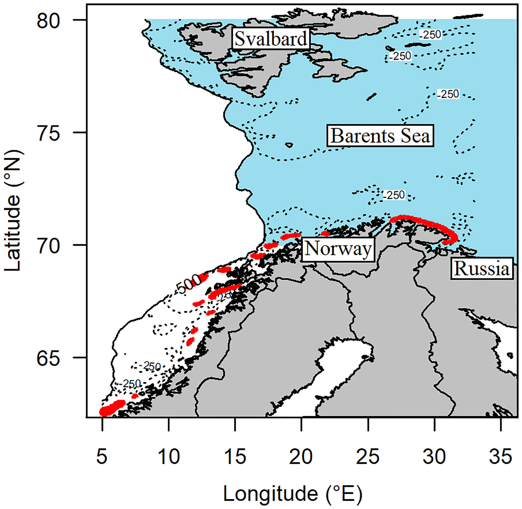
Figure 1 Map of the coast of Norway, Russia, Svalbard, and the Barents Sea. Blue area represents the recruitment area considered in the simulations, and red areas the simulated spawning grounds of NEA cod along the Norwegian coast. Isobaths for 250 and 500 m are shown in dotted and full lines.

where T_e,i, T_l,i, and T_pl,i are the egg, larvae, and post-larvae (larvae of length > 18 mm) developmental stage duration of the ith super-individual, respectively; and m_e, m_l, and m_pl are the daily mortality rates for egg, larvae, and post-larvae, respectively, based on averaged daily mortality rates for each developmental stage: 0.17 day⁻¹ for eggs, 0.075 day⁻¹ for larvae, and 0.025 day⁻¹ for post-larvae (Sundby et al., 1989; Langangen et al., 2013).

Patchiness

To quantify the accumulation of particles into patches and the potential role of patchiness for cod recruitment, we choose to investigate the distribution of cod ELS in four specific years (1965, 1969, 1979, and 1989) that could capture differences in drifting areas based on low (1965 and 1969) and high (1979 and 1989) North Atlantic Oscillation (NAO) values (Hidalgo et al., 2012). The years were also characterized by low (1965 and 1979) and high (1969 and 1989) ambient temperatures for the particles, influencing growth and the location at which the juvenile would settle after reaching a length of 50 mm. Furthermore, we investigated at different days during the year to assess the effect of dispersion during the drift phase. We considered three different dates referred as “snapshot day”: day 62 (early May) directly after the end of the spawning season, day 92 (early June) approximately at the day of metamorphosis, and day 122 (early July) approximately half-way through pelagic drift period. At the snapshot day, each super-individual was localized in a grid composed of geographical cells of equivalent size based on the drifting simulation scale of 4 km. First, we assessed whether the super-individual was not “stranded” by checking if the particle had moved from its previous day. Stranded super-individuals were removed from the subsequent calculations. We then calculated the concentration of super-individuals per cell. Next, we determined a concentration threshold for patchiness, i.e., patchiness threshold, based on the statistical distribution of super-individuals cell concentration, and corresponding to the mean concentration plus one standard deviation (Trudnowska et al., 2016). This procedure was performed for each snapshot day and for each analyzed year. Cells with a super-individual concentration higher than the patchiness threshold were flagged as “patch”, whereas the other cells were flagged as “non-patch”. On the geographic grid consisting of cells identified as “patch” and “non-patch”, we used a connected-component labeling algorithm from the R library SDMTools (VanDerWal et al., 2019; R Core Team, 2020). “Patch” cells that shared a physical border were identified as belonging to one single and continuous patch (Figure 2). “Patch” cells that were geographically separated by at least one “no-patch” cells were considered as belonging to separate patches (Figure 2). To investigate the effect of the cell size on the patch detection capacity, we simulated the patch recognition procedure for cells of increasing size, i.e., patch cell size: 8, 16, and 32 km, (Figures 2A–C).

FIGURE 2

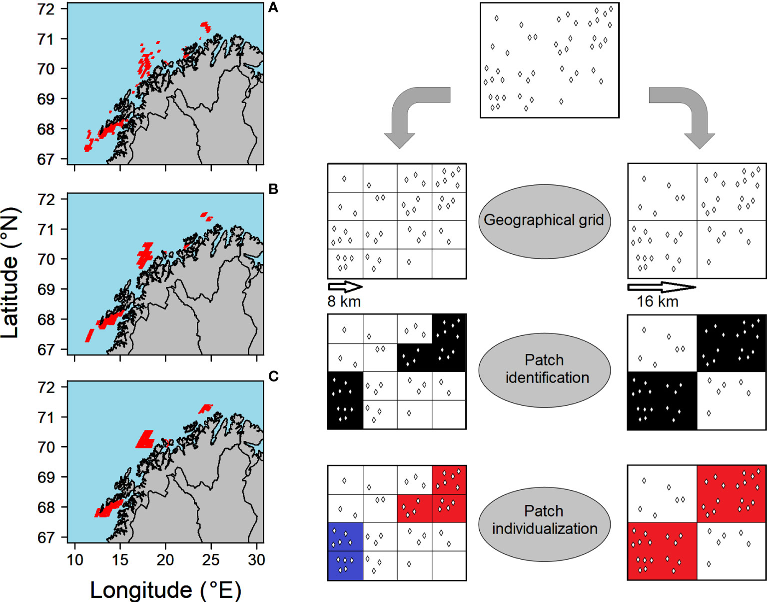
Figure 2 Maps of identified patches (red) along the Norwegian coast at day 62 during the year 1969 for the 8-km patch cell size (A), 16-km patch cell size (B), and 32-km patch cell size (C). Super-individuals (diamonds) in geographical grids of increasing size. Visual example of the patch identification algorithm based on a hypothetical particles spatial distribution. First, super-individuals are assigned into spatial cells of similar size (8 or 16 km). Second, cells with a super-individual density higher than the patch minimum density value are identified (in black). Third, the connected components algorithm individualize patches (in blue and red) based on the presence of a common spatial boundary.

Once the patches were identified and individualized, and to assess the contribution of patches to the abundance of recruited individuals, we calculated the percentage of recruits from super-individuals originating from patches to the total abundance of recruits based on Equation (2):

$\begin{array}{ll}{P}_{i,k,l,m}=\frac{{\sum }_{j=1}^n{A}_{surv,i,j,k,l,m}}{{\sum }_{J=1}^N{A}_{surv,l}} \times 100& \text{(Eq. 2)}\end{array}$

where P_i,k,l,m is the percentage of recruits from super-individuals originating from the ith patch based on the sum of A_{surv,i,j,k,l,m} of each jth recruited super-individual present in the ith patch for the kth snapshot day, lth year, and mth patch cell size. A_surv,l is the corresponding total abundance of all recruited super-individuals per lth year simulated inside the Barents Sea. The sum of P_i,k,l,mover all patches represents the percentage of recruits from super-individuals originating from all detected patches to the total abundance of recruits.

Spatial resolution of patches

We wanted to investigate which spatial sampling resolution may be required to uncover the patchiness in cod ELS in the field. For this, we assessed the average size of patches for each year, snapshot day, and patch cell size, expressed as the number of cells composing a patch, i.e., patch spatial resolution, contributing to recruitment. First, a representation of the patch physical size was assessed using Equation (3):

$\begin{array}{ll}Siz{e}_{patc{h}_{i,k,l,m}}=\sqrt{N_{cel{l}_{i,k,l,m}}*Siz{e}_{cel{l}_m}^2}& \text{(Eq. 3)}\end{array}$

where we considered the representative size of a patch Size_patchi,k,l, in kilometers, based on the squared root of the product of  N_celli,j,k,l; the number of cells, composing the ith patch, at the kth day, lth year, and mth patch cell size; and the area of the patch cell on a two-dimensional space $Siz{e}_{cel{l}_m}^2$. Second, as different patches did not contribute in equal manner to the recruitment, we developed an index for the patch spatial resolution that is the most contributing to recruitment. For this, we assessed the average cell number in a patch taking into account the patch contribution to recruitment (Patch recruitment Specific Resolution, PSR) [Equation (2)] using Equation (4):

$\begin{array}{ll}PS{R}_{k,l,m}=\sum _{i=1}^n\left(\frac{Siz{e}_{patc{h}_{i,k,l,m}}*P_{i,k,l,m}}{{\sum }_{i=1}^n{P}_{i,k,l,m}}\right)*\frac{1}{Siz{e}_{cel{l}_m}}& \text{(Eq. 4)}\end{array}$

where PSR_k,l,m is the average number of cells in a patch weighted by the recruitment contribution of the patch at the kth day, lth year, and mth patch cell size. For any cell size, we interpreted the PSR value lower than 2, i.e., less than an average of two cells, as the corresponding cell size was larger than the “real” size of the most contributing patches to recruitment. In this case, the considered cell size would be inadequate if used as a sampling distance interval in the event of a field campaign. There would be a chance to miss contributing patches, these being most likely smaller than the sampling interval. PSR values higher than 2 were interpreted as the considered cell size was smaller than the “real” size of the most contributing patches to recruitment. In this case, if the cell size is used as a sampling distance interval, then there would be a higher chance to assess the patchy structure in a field campaign. Finally, PSR values higher than 4 indicated that the considered cell size was considerably smaller than the “real” size of the most contributing patches. It also indicated that a larger cell size could be adequate as sampling distance interval to assess the patchiness in the field, considering that four cells of 8 km composes a cell of 16 km.

Results

On the basis of the simulations, we focused on three main results: 1) the yearly difference in percentage of recruits from super-individuals originating from patches to the total abundance of recruits (Figure 3A); 2) the PSR values depending on the patch cell size, day, and year simulated (Table 1); and 3) the difference and evolution of the percentage of recruits originating from patches to the total abundance of recruits at different times of the drifting period (Figure 3B).

FIGURE 3

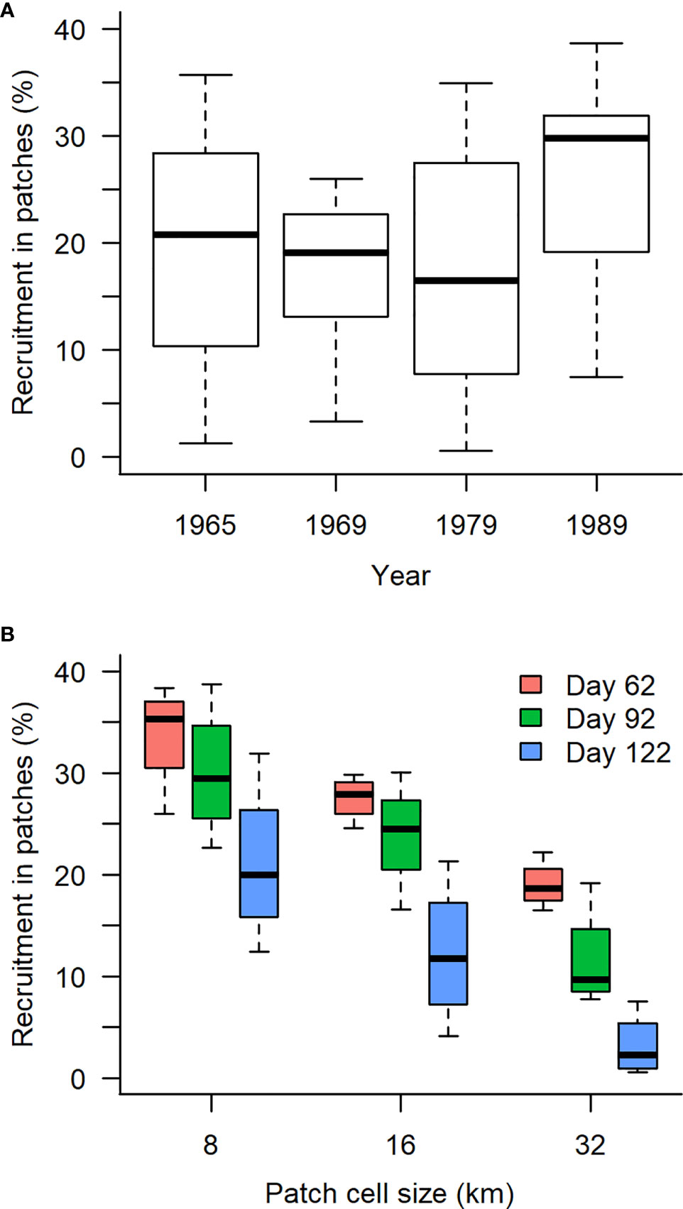
Figure 3 Box and whiskers of the percentage of recruits from super-individuals originating from patches to the total abundance of recruits for (A) the different simulated year (all patch cell sizes and days of snapshot pooled) and (B) patch cell size and day of snapshot (all years pooled). Thick black line indicates median of the distribution, the edges of the box are the 25% and 75% percentiles of the distribution, and the whiskers represent the minimum and maximum values of the distribution.

TABLE 1

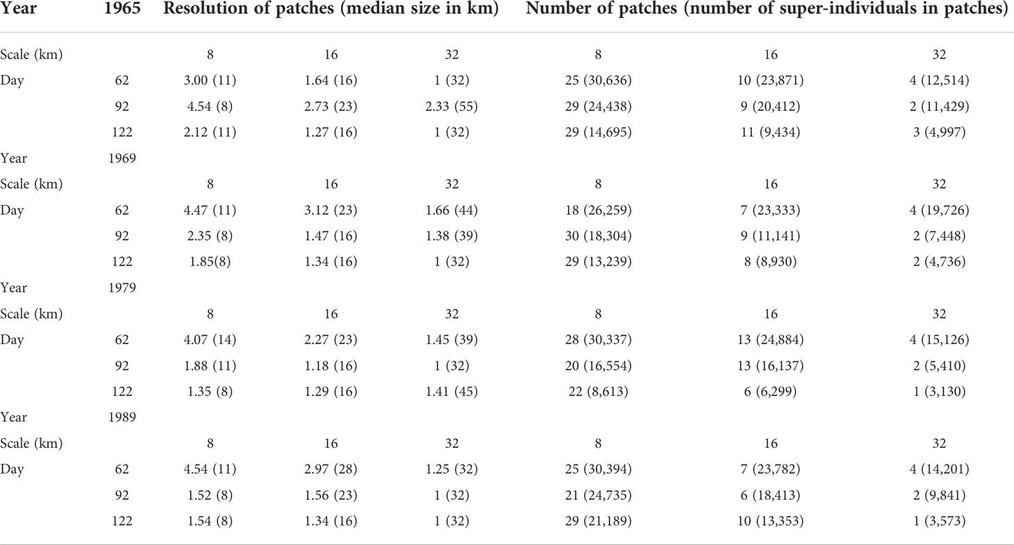
Table 1 PSR values of patches landscape and their respective median size in kilometers, and the number of patches detected with their respective number of super-individuals according to the different scales, snapshot days, and years simulated.

The percentage of recruits originating from patches of scales from 8 to 32 km to the total abundance of recruits varied between years depending on the patch size and the snapshot date. The percentage was highest in 1989 (38.7%) and lowest in 1979 (0.6%) with an average value across years of 20.4% (Figure 3A). The difference between the minimum and maximum within years was highest in 1965 (34.4%) and lowest in 1969 (22.6%).

For all days of snapshots and all years, the number of patches detected decreased with increasing patch cell size (Figure 3B and Table 1). At 8-km cell size, the number of patches ranged between 18 and 29, reducing to between 6 and 13 at 16 km and between 1 and 4 at 32 km. There was no obvious trend in the number of patches with increasing dates of snapshot (Table 1). For example, the highest number of detected patches at the scale of 8 km was detected at day 62 for year 1979, at day 92 for year 1969, and at day 122 for years 1965 and 1989.

PSR values, indicating the average number of cells in patches most contributing to the number of recruits, varied according to day, year, and the cell size. Patches represented by more than two cells was reached in seven of the 12 different simulations (4 years with three snapshot dates each) using a patch cell size of 8 km. This suggested that, more than half of the simulations, an 8-km sampling interval would be sufficient to detect patches, contributing to recruitment in the field. At the 16-km cell size, four of the 12 simulations showed a PSR value bigger than 2. This included mostly simulations with snapshot day 62, except for day 92 in 1965. Hence, a 16-km sampling interval would be sufficient to detect patches, contributing to recruitment in the field in the start of the drifting season. Finally, at the cell size of 32 km, the simulations almost never represented patches with more than two grid cells, except for snapshot day 92 in 1965 (Table 1). This suggested that a 32-km sampling interval would predominantly not be sufficient to detect patches contributing to recruitment in the field. As expected, the mean size of patches increased with increasing cell size and ranged from 10 to 55 km (Table 1). In general, the mean size of patches decreased with increasing snapshot day, expect for 1965, where the mean size of patches did not show any clear trend over the drifting period.

The percentage of recruits from super-individuals originating from patches to the total abundance of recruits varied depending on the snapshot day and scale size of the simulation. Overall, the percentage decreased as the day of snapshot increased independently of the patch cell size (Figure 3B). However, the percentage decrease could not be justified by a reduction in the recruited particles inside patches but more simply explained by fewer particles located in patches (Table 1). Less particles in patches were related with more particles outside patches and thus suggested a more homogeneous spatial distribution of particles as day of snapshot increased. The percentage of recruits from super-individuals originating from patches also decreased as the cell size increases (Figure 3B). The decrease suggested that a part of the recruits was distributed inside patches that were progressively no longer detected as the cell size increased. At the 32-km cell size, contribution to recruitment inside patches represented at maximum 22.2%, 19.2%, and 17.5% for day 62, 92, and 122, respectively, compared to 38.4%, 38.7%, and 31.9% at the 8-km cell size. This suggested that the reduction of the number of patches associated with increasing cell size (Table 1) did not correspond to an aggregation of small spatially independent patches into larger patches, but that a part of the recruits failed to be detected at the largest scale compared to that at the smallest scale.

Discussion

In this study, we detected patches of simulated drifting particles representing super-individuals of NEA cod ELS along the Norwegian coast using a connected-component labeling algorithm. Our results showed that, based on drift trajectories and average mortality rates, the percentage of recruits from super-individuals originating from patches from 8 to 32 km to the total abundance of recruits was, on average, 20.4% but varied based on year, time during the drifting season, and the size of patches. In addition, our results showed that an increase in spatial scales of patches resolved from 8 to 32 km led to a decreasing number of detected patches and a reduction in the number of cell composing the patches most contributing to recruitment (PSR). Finally, the later the snapshot day, the lesser super-individuals were located inside the patches. It suggests that super-individuals tended to leave patches over the drifting period and that super-individuals became more homogenously distributed in space over time.

Our study, based on a hydrographic drift model, assessed patchiness as created by physical processes such as oceanographic eddies, fronts, or filaments. During the drift simulation, horizontal diffusion from spatial scales not resolved by the ocean model was not taken into account. Horizontal diffusion has been highlighted as a potential source of error for destination in forward-in-time tracking modeling (Batchelder, 2006). Subgrid-scale processes, simulated by horizontal diffusion, could potentially influence local concentration of particles that we used to assess the patchy condition of geographic cells and the location of settlement, i.e., end-points of drift. However, results from particle tracking models assessing the effect of horizontal diffusion on drift trajectories at both regional and wide scale showed a limited effect on dispersion of particles (Torgersen and Huse, 2005; Espinasse et al., 2017). We consider the assumption of no extra horizontal diffusion acceptable for our purpose as the spatial resolution of the ocean model is relatively high. The sizes of detected patches were in the mesoscale range (10–100 km; Vogedes et al., 2014) and were within the sizes of observed zooplankton patches along the Norwegian coast and in the Barents Sea (Trudnowska et al., 2016; Basedow et al., 2019; Weidberg et al., 2022). Study of patchiness in zooplankton suggested an increasing number of patches associated with a decreasing patch size (Piontkovski et al., 1997). Observations from other marine systems indicate that smaller patches, i.e., maximum 5 km in size, may actually represent the dominating part of zooplankton patches (Piontkovski et al., 1997; Tsuda et al., 2000; Robinson et al., 2021). As a consequence, our results likely underestimate the total patchiness and the effect of patchiness on the recruitment of NEA cod. Furthermore, we only accounted for patches created by physical conditions and not by biological phenomenon, e.g., active aggregating behavior of ELS individuals, variation in availability of food, or predator pressure inside patches. This may potentially lead to underestimation of the patch effect on recruitment. Nevertheless, we can consider our results as a baseline describing the contribution of patches to recruitment through drift and ambient temperature.

According to our results, the percentage of recruits from super-individual originating from patches of scales from 8 to 32 km to the total abundance of recruits varied between the simulated years from a minimum of 0.6% to a maximum of 38.7% with an average of 20.4%. The yearly difference in percentages in patches suggested that the effect of potential variation in mortality rates between patches, i.e., small-scale spatial heterogeneity in mortality (Langangen et al., 2014), on recruitment would vary between years. Hence, patchiness may have a relevant effect on the inter-annual variation in NEA cod recruitment, depending on the survival within, between, and outside the patches. However, the variation in survival at the simulated spatial scales is currently unknown and would require further investigation. Furthermore, our results showed that the closer the super-individuals are getting to the recruitment period in October, the more the super-individuals are spatially homogeneously dispersed. It suggests that, close to the spawning dates (or due to patchy spawning sites; Figure 1), patchiness was more prevalent and that small-scale effects may be stronger at an early date than later in the season where dispersion has rendered the distribution of particles more homogeneously. Simulated years were selected to represent different climatic (high and low NAO) and temperature conditions affecting the fate of the super-individuals. Our results were not tested statistically because of the mechanistic nature of our model. However, we note that the percentage of recruits from super-individuals staying in patches appeared higher in 1989, a year characterized by high NAO and corresponding high ambient temperature for the super-individuals. High NAO period has previously been associated with an eastern spatial distribution of NEA cod ELS inside the Barents Sea, as compared to a low NAO period (Hidalgo et al., 2012). In our model setup, a drift farther to the east of the Barents Sea would increase the chances of super-individuals to end up in the defined recruitment area. In addition, high ambient drift temperatures would result in a faster stage development and, therefore, a lower accumulated mortality. Together, a high NAO and high ambient temperatures may be an explanation for a higher predicted recruitment in 1989.

The increase in patch cell size from 8 to 32 km was associated with decreases in the number of detected patches (as illustrated in Figure 2), the number of cells constituting a patch, and the percentage of recruits from super-individuals originating from patches to the total abundance of recruits. This result suggests that, in the case of an observation campaign with a sampling interval of 8 km in the field, a sub-sampling equivalent a sampling interval of 32 km (one of the four stations) would result in a decrease in the number of patchy structure observed and a more homogeneous observed spatial distribution of individuals. The decrease in the percentage of recruits originating from patches to the total abundance of recruits suggests that, for example, few 32-km cell–sized patches contributed to the recruitment compared to patches of smaller cell size, e.g., 8 km. In previous studies of recruitment of cod ELS, the effects of local variability in mortality rates have been discussed (Hjermann et al., 2007; Langangen et al., 2017). Our results indicate at what spatial scale such variability in mortality may take place to have a relevant impact on recruitment. Our study suggests that the few patches with a size over 30 km contributed less to recruitment than patches of smaller sizes, in the order of 10 km or smaller. It has been a major concern that, with respect to year-class loss associated with mass mortality events such as oil spills, parts of the year-class isolated in patches can have a lower than average future mortality, hence contributing disproportionally to recruitment (Langangen et al., 2017). Here, we illustrate that potential mortality variations on spatial scales down to 8 km, the smallest size of patch detected, may impact as much as 38.7% of the recruitment and can thus be relevant in understanding the year-class formation. However, as the recruitment originated from patches continuously increased with reduction in cell size, our results were limited by the horizontal drift resolution of the model and potentially suggest that the model setup with a 4-km grid resolution did not resolve important subgrid-scale processes (Torgersen and Huse, 2005; Batchelder, 2006; Espinasse et al., 2017).

In conclusion, the individual-based drifting model predicted that, on average, 20% of the NEA cod recruits were located in patches. The percentage values varied according to 1) year, likely due to difference in drifting trajectories; 2) day of the year with later days being associated with a decrease in patchiness of the super-individuals; and 3) resolution of patches with high percentage values associated our finest resolved scale of 8 km. To further investigate the significance of scale for the recruitment of NEA cod, higher spatial resolution drift models can be helpful, however, at a computational cost. To get a full overview of the potential cohort and population level impacts of heterogeneity in spatial mortality and other mass mortality events, the exploration of spatial mortality landscape should then remain under a scale of 10 km, both numerically and in the field. Therefore, we advocate for a fine sampling resolution to help resolve heterogeneity in spatial mortality for ELS of NEA cod as well as potentially other species with similar drifting ELS, e.g., Norwegian spring-spawning herring (Clupea harengus; Krysov and Røttingen, 2011).

Data availability statement

The raw data supporting the conclusions of this article will be made available by the authors, without undue reservation.

Author contributions

ØL and FV provided the coupled physical-biological drift model simulation. ND developed the methods related to patches and performed numerical calculations based on patch detection and wrote the first draft of the manuscript. All authors discussed, commented and revised the final version of the manuscript.

Funding

This study was funded by the Research Council of Norway under the project OILCOM (#RCN: 255487/E40).

Conflict of interest

The authors declare that the research was conducted in the absence of any commercial or financial relationships that could be construed as a potential conflict of interest.

Publisher’s note

All claims expressed in this article are solely those of the authors and do not necessarily represent those of their affiliated organizations, or those of the publisher, the editors and the reviewers. Any product that may be evaluated in this article, or claim that may be made by its manufacturer, is not guaranteed or endorsed by the publisher.

References

Basedow S. L., McKee D., Lefering I., Gislason A., Daase M., Trudnowska E., et al. (2019). Remote sensing of zooplankton swarms. Sci. Rep. 9 (1), 686. doi: 10.1038/s41598-018-37129-x

PubMed Abstract | CrossRef Full Text | Google Scholar

Batchelder H. P. (2006). Forward-in-time-/Backward-in-Time-Trajectory (FITT/BITT) modeling of particles and organisms in the coastal ocean. J. Atmosperic Oceanic Technol. 23, 727–741. doi: 10.1175/JTECH1874.1

CrossRef Full Text | Google Scholar

Bergstad O. A., Jørgensen T., Dragesund O. (1987). Life history and ecology of the gadoid resources of the barents Sea. Fish. Res. 5 (2-3), 119–161. doi: 10.1016/0165-7836(87)90037-3

CrossRef Full Text | Google Scholar

Björnsson B., Steinarsson A., Árnason T. (2007). Growth model for Atlantic cod (Gadus morhua): Effects of temperature and body weight on growth rate. Aquaculture 271 (1-4), 216–226. doi: 10.1016/j.aquaculture.2007.06.026

CrossRef Full Text | Google Scholar

Brentnall S. J., Richards K. J., Brindley J., Murphy E. (2003). Plankton patchiness and its effect on large-scale productivity. J. Plankton Res. 25 (2), 121–140. doi: 10.1093/plankt/25.2.121

CrossRef Full Text | Google Scholar

Castaño-Primo R., Vikebø F. B., Sundby S. (2014). A model approach to identify the spawning grounds and describing the early life history of northeast Arctic haddock (Melanogrammus aeglefinus). ICES J. Mar. Sci. 71 (9), 2505–2514. doi: 10.1093/icesjms/fsu078

CrossRef Full Text | Google Scholar

Ellertsen B., Fossum P., Solemdal P., Sundby S., Tilseth S. (1987)The effects of biological and physical factors on the survival of arcto-Norwegian cod and the influence on recruitment variability. In: Proceedings of the third soviet-Norwegian symposium, Murmansk (Bergen, Norway) (Accessed 26-28 May 1986).

Google Scholar

Espinasse B., Tverberg V., Basedow S. L., Hattermann T., Nøst O. A., Albretsen J., et al. (2017). Mechanisms regulating inter-annual variability in zooplankton advection over the lofoten shelf, implication for cod larvae survival. Fish. Oceanogr. 26 (3), 299–315. doi: 10.1111/fog.12193

CrossRef Full Text | Google Scholar

Fey D. P., Szkudlarek-Pawełczyk A. (2022). Precision of larval herring abundance and body length assessments when sampling with BONGO nets for spawning site mapping. Fish. Res. 246, 106165. doi: 10.1016/j.fishres.2021.106165

CrossRef Full Text | Google Scholar

Folkvord A. (2005). Comparison of size-at-age of larval Atlantic cod (Gadus morhua) from different populations based on size- and temperature-dependent growth models. Canadian J. Fisheries Aquatic Sci. 62(5), 1037–1052. doi: 10.1139/F05-008

CrossRef Full Text | Google Scholar

Genin A. (2004). Bio-physical coupling in the formation of zooplankton and fish aggregations over abrupt topographies. J. Mar. Syst. 50, 3–40. doi: 10.1016/j.jmarsys.2003.10.008

CrossRef Full Text | Google Scholar

Grünbaum D. (2012). The logic of ecological patchiness. Interface Focus 2, 150–155. doi: 10.1098/rsfs.2011.0084

PubMed Abstract | CrossRef Full Text | Google Scholar

Hidalgo M., Gusdal Y., Dingsør G. E., Hjermann D. O., Ottersen G., Stige L. C., et al. (2012). A combination of hydrodynamical and statistical modelling reveals non-stationary climate effects on fish larvae distributions. Proc. R. Soc. B: Biol. Sci. 279, 275–283. doi: 10.1098/rspb.2011.0750

CrossRef Full Text | Google Scholar

Hjermann D.Ø., Melsom A., Dingsør G. E., Durant J. M., Eikeset A. M., Røed L. P., et al. (2007). Fish and oil in the lofoten-barents Sea system: Synoptic review of the effects of oil spills on fish populations. Mar. Ecol. Prog. Ser. 339, 283–299. doi: 10.3354/meps339283

CrossRef Full Text | Google Scholar

Houde E. D. (2008). Emerging from hjort's shadow. J. Northwest Atlantic Fishery Sci. 41, 53–70. doi: 10.2960/J.v41.m634

CrossRef Full Text | Google Scholar

Kareiva P. (1990). Population dynamics in spatially complex environments: Theory and data. Philos. Trans. R. Soc. London Ser. B: Biol. Sci. 330 (1), 175–190. doi: 10.1098/rstb.1990.0191

CrossRef Full Text | Google Scholar

Krysov A. I., Røttingen I. (2011). “Herring,” in The barents Sea: Ecosystem, resources, management half a century of Russian-Norwegian cooperation. Eds. Jakobsen T., Ozhigin V. K. (Trondheim: Tapir Academic Press), 215–224.

Google Scholar

Langangen Ø., Olsen E., Stige L. C., Ohlberger J., Yaragina N. A., Vikebø F. B., et al. (2017). The effects of oil spills on marine fish: Implication of spatial variation in natural mortality. Mar. pollut. Bull. 119, 102–109. doi: 10.1016/j.marpolbul.2017.03.037

PubMed Abstract | CrossRef Full Text | Google Scholar

Langangen Ø., Ottersen G., Ciannelli L., Vikebø F. B., Stige L. C. (2016). Reproductive strategy of a migratory fish stock: implications of spatial variations in natural mortality. Can. J. Fish. Aquat. Sci. 73, 1742–1749. doi: 10.1139/cjfas-2015-0321

CrossRef Full Text | Google Scholar

Langangen Ø., Stige L. C., Yaragina N. A., Ottersen G., Vikebø F. B., Stenseth N. C. (2014). Spatial variations in mortaltiy in pelagic early life stages of a marine fish (Gadus morhua). Prog. Oceanogr. 127, 96–107. doi: 10.1016/j.pocean.2014.06.003

CrossRef Full Text | Google Scholar

Langangen Ø., Stige L. C., Yaragina N. A., Vikebø F. B., Bogstad B., Gusdal Y. (2013). Egg mortality of northeast Arctic cod (Gadus morhua) and haddock (Melanogrammus aeglefinus)†. ICES J. Mar. Sci. 71 (5), 1129–1136. doi: 10.1093/icesjms/fst007

CrossRef Full Text | Google Scholar

Lien V. S., Gusdal Y., Albertsen J., Melsom A., Vikebø F. (2013). Evaluation of a Nordic seas 4 km numerical ocean model hindcast archive (SVIM), 1960-2011. Fisken og Havet 7, 81. Available at: http://hdl.handle.net/11250/113861.

Google Scholar

Lough R. G., Caldarone E. M., Rotunno T. K., Broughton E. A., Burns B. R., Buckley L. J. (1996). Vertical distribution of cod and haddock eggs and larvae, feeding and condition in stratifiedand mixed waters on southern georges bank, may 1992. Deep-Sea Res. Part Ii-Topical Stud. Oceanogr. 43, 1875–1904. doi: 10.1016/S0967-0645(96)00053-7

CrossRef Full Text | Google Scholar

McGurk M. D. (1986). Natural mortality of marine pelagic fish eggs and larvae - role of spatial patchiness. Mar. Ecol. Prog. Ser. 34 (3), 227–242. doi: 10.3354/meps034227

CrossRef Full Text | Google Scholar

Methven D. A., Schneider D. C., Rose G. A. (2003). Spatial pattern and patchiness during ontogeny: Post-settled gadus morhua from coastal Newfoundland. ICES J. Mar. Sci. 60 (1), 38–51. doi: 10.1006/jmsc.2002.1315

CrossRef Full Text | Google Scholar

Opdal A. F., Vikebø F. B., Fiksen Ø. (2011). Parental migration, climate and thermal exposure of larvae: spawning in southern regions gives northeast Arctic cod a warm start. Mar. Ecol. Prog. Ser. 439, 255–262. doi: 10.3354/meps09335

CrossRef Full Text | Google Scholar

Ottersen G., Bogstad B., Yaragina N. A., Stige L. C., Vikebø F. B., Dalpadado P. (2014). A review of early life history dynamics of barents Sea cod (Gadus morhua). ICES J. Mar. Sci. 71 (8), 2064–2087. doi: 10.1093/icesjms/fsu037

CrossRef Full Text | Google Scholar

Piontkovski S. A., Williams R., Peterson W. T., Yunev O. A., Minkina N. I., Vladimorov V. L., et al. (1997). Spatial heterogeneity of the planktonic fields in the upper mixed layer of the open ocean. Mar. Ecol. Prog. Ser. 148, 145–154. doi: 10.3354/meps148145

CrossRef Full Text | Google Scholar

R Core Team (2017). “R: A language and environment for statistical computing,” (Vienna, Austria: R Foundation for Statistical Computing). version: 3.6.3. Available at: https://www.R-project.org/.

Google Scholar

Robinson K. L., Sponaugle S., Luo J. Y., Gleiber M. R., Cowen R. K. (2021). Big or small, patchy all: Resolution of marine plankton patch structure at micro- to submesoscales for 36 taxa. Sci. Adv. 7 (47), eabk2904. doi: 10.1126/sciadv.abk2904

PubMed Abstract | CrossRef Full Text | Google Scholar

Scheffer M., Baveco J. M., DeAngelis D. L., Rose K. A., van Nes E. H. (1995). Super-individuals a simple solution for modelling large populations on a individual basis. Ecol. Model. 80 (2-3), 161–170. doi: 10.1016/0304-3800(94)00055-M

CrossRef Full Text | Google Scholar

Shchepetkin A. F., McWilliams J. C. (2005). The regional oceanic modeling system (ROMS): A split-explicit, free-surface, topography-following-coordinate oceanic model. Ocean Model. 9, 347–404. doi: 10.1016/j.ocemod.2004.08.002

CrossRef Full Text | Google Scholar

Sundby S. (1997). Turbulence and ichtyoplankton: influence on vertical distributions and encounter rates. Scientia Marina 61, 159–176.

Google Scholar

Sundby S., Bjørke H., Soldal A., Olsen S. (1989). Mortality rates during the early life stages and year-class strength of northeast Arctic cod (Gadus morhua l.). ICES Mar. Sci. Symp. 191, 351–358.

Google Scholar

Sundby S., Nakken O. (2008). Spatial shifts in spawning habitats of arcto-Norwegian cod related to multidecadal climate oscillation and climate change. Ices J. Mar. Sci. 65 (6), 953–962. doi: 10.1093/icesjms/fsn085

CrossRef Full Text | Google Scholar

Thygesen U. H., Ådlandsvik B. (2007). Simulating vertical turbulent dipersal with finite volumes and binned random walks. Mar. Ecol. Prog. Ser. 347, 145–153. doi: 10.3354/meps06975

CrossRef Full Text | Google Scholar

Torgersen T., Huse G. (2005). Variability in retention of Calanus finmarchicus in the Nordic seas. Ices J. Mar. Sci. 62, 1301–1309. doi: 10.1016/j.icesjms.2005.05.016

CrossRef Full Text | Google Scholar

Trudnowska E., Gluchowska M., Beszczynska-Möller A., Blachowiak-Samolyk K., Kwasnieski S. (2016). Plankton patchiness in the polar front region of West spitsbergen shelf. Mar. Ecol. Prog. Ser. 560, 1–18. doi: 10.3354/meps11925

CrossRef Full Text | Google Scholar

Tsuda A., Sugisaki H., Kimura S. (2000). Mosaic horizontal distributions of three species of copepods in the subarctic pacific during spring. Mar. Biol. Res. 137, 683–689. doi: 10.1007/s002270000338

CrossRef Full Text | Google Scholar

VanDerWal J., Falconi L., Januchowski S., Shoo L., Storlie C. (2019). SDMTools: Species distribution modelling tools: Tools for processing data associated with species distribution modelling exercises. version: 1.1-221.2. Available at: https://cran.r-project.org/web/packages/SDMTools/index.html.

Google Scholar

Vikebø F. B., Broch O. J., Endo C. A. K., Frøysa H. G., Carroll J., Juselius J., et al. (2021). Northeast Arctic cod and prey match-mismatch in a high-latitude spring-bloom system. Front. Mar. Sci. 8. doi: 10.3389/fmars.2021.767191

PubMed Abstract | CrossRef Full Text | Google Scholar

Vogedes D., Eiane K., Båtnes A. S., Berge J. (2014). Variability in Calanus spp. abundance on fine- to mesoscales in an Arctic fjord: Implications for little auk feeding. Mar. Biol. Res. 10 (5), 437–448.

Google Scholar

Weidberg N., Hernandez N. S., Renner A. H. H., Falk-Petersen S., Basedow S. L. (2022). Large Scale patches in Calanus finmarchicus and associated hycrographic conditions off the lofoten archipelago. J. Mar. Syst. 227, 103697. doi: 10.1016/j.jmarsys.2021.103697

CrossRef Full Text | Google Scholar