Three-dimensional smoothed particle hydrodynamics modeling of near-shore current flows over rough topographic surface

Introduction

After the ocean wave breaks in the surf zone, it propagates to the coastal area in the form of a near-shore current. Depending on local bathymetry and coastal structures, these near-shore currents can demonstrate both shore-parallel and shore-cross flow features. They can influence the navigation safety, cause sedimentation, destabilize coastal structure and, in the longer term, shape the evolution of coastal morphology. A sound understanding of these flows and their consequences could help in the sustainable design and safety operation of coastal environment. Therefore, these free surface flows have significant practical importance and theoretical complexity, due to their relatively shallow depths over a rough bed boundary. The featured three-dimensional (3D) turbulence and large-scale secondary flow structures also play an important role in the cross-sectional flow dynamics. In studying these turbulence flow structures, it is imperative to consider the existence of the secondary current, and the lateral and vertical velocity and shear stress distributions, because they all reflect the internal transfers of the flow momentum and energy.

For the study of these near-shore current flows or similar types, there exist quite a few documented numerical works and the following examples are not exhaustive. For example, Chen and Tsai (2012) adopted a finite-volume method with adequate numerical algorithms for computing the wave transformation based on the hyperbolic time-dependent mild-slope equations involving wave breaking. Both the predictor-corrector scheme and the time-staggered leapfrog scheme were employed to discretize the governing equations. Nam et al. (2009) developed a 2D numerical model of cross-shore variations in mean water elevation and sediment transport in the shores and swash zones. The multi-directional random wave transformation model based on an energy balance equation was employed with an improved description of energy dissipation due to wave breaking. Tang et al. (2017) and Zhang et al. (2020) developed a numerical model to simulate hydrodynamics (including waves, currents, and mean water level), cross-shore sediment transport, and beach profile evolution in the near-shore assuming negligible longshore transport gradients, with different sub-modules describing each individual process. Brakenhoff et al. (2020) quantified the importance of ripple- and megaripple-related roughness for modeled hydrodynamics and sediment transport on the wave- and tide-dominated Ameland ebb-tidal delta in the north of the Netherlands, and several types of bedform-related roughness predictors were evaluated using a Delft3D model. Besides, Yao et al. (2022) used a 3D numerical wave tank based on OpenFOAM, in which volume averaged Reynolds averaged Navier-Stokes equation (VARANS) equations are solved for the two-phase incompressible flow with the k-ω SST model for the turbulence closure and VOF method for tracking the free surface. The reef surface with high friction is modeled by using a porous media model in the VARANS equations.

The mesh-free smoothed particle hydrodynamics (SPH) technique has been used for the simulation of a wide range of computational fluid dynamics (CFD) applications in the recent decades (Monaghan, et al., 1994). Unlike the traditional mesh-based method, SPH is a pure Lagrangian technique in which the fluid domain is discretized into a set of particles carrying various physical properties, and these particles move following the governing equations subject to particle interaction models. Due to its capability and flexibility of simulating various complex free surface flows, SPH is becoming a competitive alternative to the mesh-based numerical approaches. Compared with SPH applications in coastal waves, the documented studies in unilateral flows such as the near-shore current are not frequent. Two benchmark studies have been found on SPH simulations of near-shore current flows. Farahani et al. (2012) used SPH for analyzing rip current flows generated by a single bar and a rip channel, in which the mean horizontal variations of rip current system and 3D circulations were studied. They revealed the wave-current interaction and flow patterns in different parts of rip channel, bar, and the trough located near shore. Lowe et al. (2019) used SPH code DualSPHysics to simulate wave breaking over two bathymetric profiles and compared to experimental flume measurements of waves, currents, and mean water levels. They numerically studied a broad range of hydrodynamic processes, ranging from the nonlinear evolution of wave shapes across the surf zone, to mean current profiles and wave runup.

In SPH simulation of near-shore flow currents, two technical difficulties are involved, including the treatment of rough bed and flow turbulence. Early studies in the form of open channel flow involved mostly a smoothed topographic surface (e.g., Fedderico et al., 2012; Meister et al., 2014), where there was no extra resistance force from the bed. This idealized condition is not applicable to coastal regions, where bed roughness elements always exist. To deal with more complex rough topographic boundaries, Džebo et al. (2014) carried out SPH modeling of dam break flow through a narrow valley, where two different ways of defining terrain roughness were used, that is, a wall-particle eddy viscosity coefficient to treat the hydraulically smooth terrain, and an elevation of mesh-node of obstacles along the valley to treat the hydraulically rough terrain. Gabreil et al. (2018) quantified the drag force induced by the bed roughness element and validated flow velocity and shear stress profiles with laboratory experiment, based on extensive 2D SPH simulations. Kazemi et al. (2020) further improved the model capacity by including an additional porous flow model, for the study of flow over and within natural gravel beds with a rough interfacial boundary. Through velocity analysis, they found a nearly S-shaped profile within the roughness layer that is important for the study on sediment motions. The latest work should be attributed to Bartzke et al. (2021), who used an SPH open-source code DualSPHysics to model the flow passing over a sphere resting on rough bed. The flow velocity profiles in the vicinity of large sphere were validated with the experimental data, which correctly reproduced the flow features and interactions in the vicinity of natural sediment grains and larger bodies. Besides, it is reported that some other mesh-free numerical methods have also adopted similar approaches for applications such as wave overtopping on a permeable breakwater, based on a Material Point Method (Harris et al., 2021).

On the other hand, when the current flows flow over a rough bed surface, especially when the flow depth is shallow, the underlying roughens elements could generate substantial turbulence and eddies. Despite the fact that SPH is a mesh-free particle-based model and equipped with solving eddy scales using SPH kernel function in a way similar to the large eddy simulation, the inclusion of an explicit turbulence model could improve model performance under the present research themes. Pioneering turbulence model for mesh-free numerical method was proposed by Gotoh et al. (2001), based on a moving particle semi-implicit approach. The proposed sub-particle-scale (SPS) turbulence model has been widely used in SPH modeling of coastal hydrodynamics. However, under some flow conditions, the SPS model was found to transfer incorrect turbulence quantifies and thus lead to large errors between numerical and experimental values (Altomare et al., 2021). A comprehensive review on various turbulent closure models was done by Violeau and Issa (2007) for their potential applications with the SPH. Alternative turbulence modeling techniques have been coupled with SPH as well. For example, Duan and Chen (2015) develop a dynamic SPS turbulence for mixing layer flows and they found the turbulent statistic profiles agreed better with experimental data than the results from a static SPS model. Besides, Wang and Liu (2020) coupled K-Epsilon model with an incompressible SPH solver for simulating turbulence under tsunami waves and much better agreement was found with the documented data if were to be compared with the original SPS model. With regards to open channel flows, Gabreil et al. (2018) found that a mixing-length-based turbulence closure could provide much more reasonable prediction of turbulence shear stresses than using the original SPS turbulence model. They state that the latter would be more efficient when dealing with transient flows in which large shear deformation occurs such as in a wave breaking, whereas for common open channel flows with much less shear deformation, SPS model tends to provide unreasonably small turbulent quantities. The validity of this study has also been explored by De Padova et al. (2013) in their 3D SPH modeling of hydraulic jump in a very large channel.

By reviewing relevant literature, it seems there lacked a detailed quantification of velocity and shear stress profiles for turbulent shallow flows over a rough bed. Considering that this type of unilateral flow is always common in coastal and near-shore areas where the flow depth is relatively shallow and the influence of physical boundaries is complex, the present study aims to develop a 3D SPH modeling technique for such a practical purpose. The model will be validated by a representative set of data collected in the laboratory chute. Different from the previous 2D SPH simulations (Gabreil et al., 2018), the present study extends the model to 3D domain, with key innovations being made in the turbulence and rough boundary modeling techniques. By reproducing an experimental flow contained in a laboratory channel, the key features of 3D unilateral current flow widely found in the coastal and near-shore areas will be investigated. Here, it should be noted that only water flow is considered in the present study, whereas more complex processes such as flow-debris interaction during extreme hydrodynamic events have been studied by Ruffini et al. (2021) using an open source DualSPHysics model coupled with the multi-physics engine CHRONO. The most recent DualSPHysics hydraulic applications were reported on a stepped spillway, where extensive comparisons between the single- and the two-phase modeling approaches have been made with regards to the skimming and the nappe flows (Gu et al., 2022).

Fundamental smoothed particle hydrodynamics methodology

SPH relies on the interpolation technique that expresses a function in the form of its values in a set of points that are disordered (Monaghan, 1994). The interpolation of given function A(r) in the SPH context is defined as

$\begin{array}{ll}A(r)={\displaystyle \int A(r)W(r^{}-r^{\prime },h)d}{r}^{\prime }& (1)\end{array}$

The integration occurs over the entire space, where W is the interpolating kernel; r is the particle position; and h is the smoothing length so the radius of particle influence domain is 2h. In SPH concept, the reference particle a interacts with the neighboring particle b within its kernel influence domain through a weighting function W(| r_ab |,h). For SPH approximation, the value of any vector or scalar of a desired particle a, and its gradient can be estimated by using the following discretized summation equations that are carried out for all the particles b within the influence domain:

$\begin{array}{ll}A(r_a)={\displaystyle \sum _b\frac{m_b}{{\rho }_b}A(r_b)W_{ab}}& (2)\end{array}$

$\begin{array}{ll}\nabla A(r_a)={\displaystyle \sum _b\frac{m_b}{{\rho }_b}}\left[A\left(r_a\right)-A\left(r_b\right)\right]\nabla {}_a{W}_{ab}& (3)\end{array}$

where m_b and ρ_b are the mass and density of the neighboring particle b; A(r_a) and A(r_b) represent the values of quantity A at point r_a and r_b, respectively; ∇A(r_a) is the gradient of the quantity; and ∇_aW_ab represents the gradient of the kernel function.

In SPH, the following mass and momentum conservation equations of the compressible Newtonian fluids are solved in a Lagrangian form:

$\begin{array}{ll}\frac{D\rho }{Dt}=-\rho \nabla ·u& (4)\end{array}$

$\begin{array}{ll}\frac{Du}{Dt}=-\frac{1}{\rho }\nabla P+g+{\upsilon }_0{\nabla }^{2}u+\frac{1}{\rho }\nabla ·{\tau }_t+\frac{1}{\rho }{\tau }_d& (5)\end{array}$

where t is the time; ρ is the fluid density; u is the particle velocity vector; P is the pressure; g is the gravitational acceleration; υ₀ is the kinematic viscosity coefficient; τ_t is the turbulence stress tensor; and τ_d is the form drag-induced shear stress from the rough bed. The fluid particle movement is therefore computed by

$\begin{array}{ll}\frac{Dr}{Dt}=u& (6)\end{array}$

By using SPH discretization Equations (2) and (3), the changing rate of density of particle a with respect to its neighboring particle b can be computed as:

$\begin{array}{ll}\frac{D{\rho }_a}{Dt}={\displaystyle \sum _b{m}_b}{u}_{ab}{\nabla }_a{W}_{ab}& (7)\end{array}$

where u_ab = u_a - u_b is defined as the velocity difference between the two particles. Similarly, all terms in the momentum Equation (5) can be transformed into SPH forms to be represented by

$\begin{array}{ll}\frac{D{u}_a}{Dt}={\displaystyle \sum _b{m}_b\left(\frac{P_a}{{\rho }_a^2}+\frac{P_b}{{\rho }_b^2}\right){\nabla }_a{W}_{}{W}_{ab}+g+{\displaystyle \sum _b{m}_b\frac{4{\upsilon }_0}{\left({\rho }_a+{\rho }_b\right)}\frac{r_{ab}·{\nabla }_a{W}_{ab}}{{\left|r_{ab}\right|}^2+{\eta }^2}{u}_{ab}}}+{\displaystyle \sum _b{m}_b\left(\frac{{\tau }_a}{{\rho }_a^2}+\frac{{\tau }_b}{{\rho }_a^2}\right)·{\nabla }_a{W}_{ab}+\frac{1}{{\rho }_a}{\left({\tau }_d\right)}_a}& (8)\end{array}$

To close the system of the governing equations for a slightly compressible fluid flow, the following equation of state is employed to determine the fluid pressure

$\begin{array}{ll}P=B\left[{\left(\frac{\rho }{{\rho }_0}\right)}^{\gamma }-1\right]& (9)\end{array}$

where $B=c_0^2{\rho }_0/\gamma$ is defined, in which c₀ is the sound speed at the reference density; ρ₀ is 1,000 kg/m³ of the reference density; and γ = 7.0 is the polytrophic constant. It was suggested by Monaghan (1994) that the minimum speed of the sound should be 10 times larger than the maximum bulk flow velocity. η in Equation (8) is a small number to avoid singularity.

In this study, the open-source code SPHysics is used (see http://www.sphysics.org). SPHysics is a free open-source SPH code that was released in 2007. It is programmed in FORTRAN and developed specifically for the free-surface hydrodynamics (Gomez-Gesteira et al., 2012). In the present study, a dynamic boundary approach is used for treating the solid wall particles (Dalrymple and Knio, 2001) and a standard periodic boundary model is adopted for the inflow and outflow boundaries. We will use the SPHysics for the simulation of shallow turbulent free surface flows over a rough bed surface, after modifying the code by adding 3D turbulent closure and rough bed models. The proposed model would be useful for studying the near-shore current flows where they encounter a rough topographic surface due to their relatively shallow flowing depths.

Three-dimensional turbulence and three-dimensional rough bed models

This section provides a modification of previous 2D SPH algorithms (Gabreil et al., 2018) for more practical applications, developing a 3D turbulence closure to address the turbulence transfer over the whole cross-sectional areas of the flow and developing a drag force model to account for the existence of roughness elements on the main bed and lateral boundaries.

Turbulence model of particle approach

In SPH, 3D flow turbulent shear stress can be modeled based on an eddy viscosity sub-particle scale (SPS) scheme of Gotoh et al. (2001) as

$\begin{array}{ll}\frac{{\tau }_{ij}}{\rho }=2{\upsilon }_t{S}_{ij}-\frac{2}{3}k{\delta }_{ij}-\frac{2}{3}{C}_I{\Delta }^2{\delta }_{ij}{\left|{\delta }_{ij}\right|}^2& (10)\end{array}$

where the turbulence eddy viscosity, υ_t=(C_sΔ)²| S |, is defined; $\Delta =\sqrt{d{x}^2+d{y}^2+d{z}^2}/3$ is the filter width; C_s is the Smagorinsky constant with an original value of 0.12; k is the SPS turbulent kinetic energy; C_I is a constant 0.0066; δ_ij is the Kronecker’s delta; and | S | is the local strain rate. However, similar to the previous 2D SPHysics study (Gabreil et al., 2018), the present 3D standard SPS turbulent model using a fixed Smagorinsky constant also predicted a much smaller shear stress value as compared with experimental data. Then alternative formulation is considered below.

Czernuszenko and Rylov (2000) proposed a simple analytical model from the generalization of Prandtl’s mixing length theory, and they obtained the mean flow velocity and shear stress distributions in a 3D non-homogeneous turbulent flow. They used the following formula to calculate the turbulent shear stress as

$\begin{array}{ll}\frac{{\tau }_{ij}}{\rho }=0.5\left(l_i^2+l_j^2\right)\left(\frac{dU}{dy}\right)\left|\frac{dU}{dy}\right|& (11)\end{array}$

It is noted above that different turbulent mixing length scales are specified in different directions by the term of $0.5\left(l_i^2+l_j^2\right)$. This term can be substituted into the present 3D SPS model, replacing the fixed product C_sΔ term in Gotoh et al. (2001), to better represent the turbulent eddy scales. In this sense, the combination of two variable turbulent length scales in different directions have been introduced rather than using only a fixed constant value. Then the modified SPS turbulence shear stresses, τ_xy, τ_xz and τ_yz in 3D can be computed as

$\begin{array}{ll}\frac{{\tau }_{xy}}{\rho }=0.5(l_x^2+l_y^2)\left(\frac{du}{dy}+\frac{dv}{dx}\right)\left|S\right|& (12)\end{array}$

where l is the mixing length in different dimensions, and similar equations can also be written in the other two coordinates. These calculated shear stresses will be substituted into the momentum Equation (5) or (8) to account for the turbulent effects.

In 3D flows, the turbulent eddies have different length scales in the streamwise, vertical and spanwise directions, referred as l_x, l_y ,and l_z, respectively. To quantify these, the cross-sectional flow areas should be divided into the middle and edge zones. In the middle zone, which is hydraulically far away from the lateral boundaries, the mixing length is only influenced by the rough bed and the water surface, whereas in the edge zones that are hydraulically close to the lateral boundaries, the mixing length is also influenced by the boundary itself. Besides, the three components of mixing length are assumed to vanish at the solid wall boundaries.

Drag force model of rough bed and lateral boundaries

In 3D shallow near-shore currents, the flow is not only influenced by the roughness elements on the topographic bed but also by those on the lateral boundaries. This section extends the 2D rough bed model of Gabreil et al. (2018) to include the drag forces induced by the roughness elements on all the solid boundaries. In a general form, the bed drag force is quantified by using the drag formula given below and then added to the momentum Equation (5) or (8), as

$\begin{array}{ll}{\tau }_d=\frac{F_d}{A_{\tau }}& (13)\end{array}$

$\begin{array}{ll}{F}_d=-\frac{1}{2}{C}_d{W}_d\rho A_{d}u\left|u\right|& (14)\end{array}$

where F_d is the drag force exerted on the fluid particle from the rough bed, which is assumed to be equal to and in the opposite direction of the force from the fluid particle acting on the bed; and A_t is the bed-parallel, planar rough area affecting the fluid particles. Furthermore, the drag force F_d will be calculated by Equation (14), where C_d is the drag coefficient, A_d is the planar cross-sectional area and W_d is a non-dimensional shape function accounting for the geometry of the bed roughness. In 3D flows, the drag forces act in the streamwise, vertical and lateral directions, respectively, but the vertical drag force is only computed on the lateral boundaries due to its dominant influence there.

To quantify the drag force from the lateral boundary elements, the following approach is referenced. As well known, the mean bed shear stress for a uniform open channel flow is represented by τ = ρgRS₀, where R is the hydraulic radius and S₀ is the bed slope. Then, it can be reasoned that the shear forces acting on the rough bed could be separated from those acting on the lateral walls. As a result, we further classify the flows into different sub-flow regions in the cross-sectional direction. Yang and Lim (1997) derived the slope of division lines, k, and linked these to the ratios of bed to wall shear velocities $\left(k=u_{bed}^{\ast }/u_{wall}^{\ast }\right)$ . By following a similar approach, the ratio of bed to wall drag forces can be quantified.

More details on quantifying the key parameters in Equations (10)–(14) can be found in the dissertation report (Gabreil, 2017).

Laboratory experiment

The laboratory experiment was carried out in a unilateral flow flume located at The University of Bradford, UK. The aim of the experimental study was to measure the flow velocity components in the streamwise, vertical and lateral directions, over a fixed uniform rough bed for a range of turbulent flow conditions. The measurements were then used to support the development of 3D SPH modeling approach for use in the shallow and turbulent free surface flows, which allows the examination of the underlying flow structures. The measurements were carried out in a 0.459-m wide and 12.6-m long rectangular flume with water recirculation system. At the upstream end, the hydraulic flume was supported on a fixed pivot joint and on another attached to an adjustable jack at the downstream end. The vertical sidewalls of the flume were composed of glasses to enable flow observation. To form a well-defined rough bed surface, the channel bed was covered by two layers of smooth plastic spheres with diameter 25.0 mm and density 1,400 kg/m³, which were arranged in a hexagonal pattern as shown in Figure 1. Four different flow conditions were selected in the experiment by using various water depths and bed slopes, as shown in Table 1. These flow conditions were selected to investigate the influence of rough bed elements on the velocity and shear stress profiles of the flows. The experimental Re number ranged approximately 11,000–43,000, so all the flows are fully turbulent.

FIGURE 1

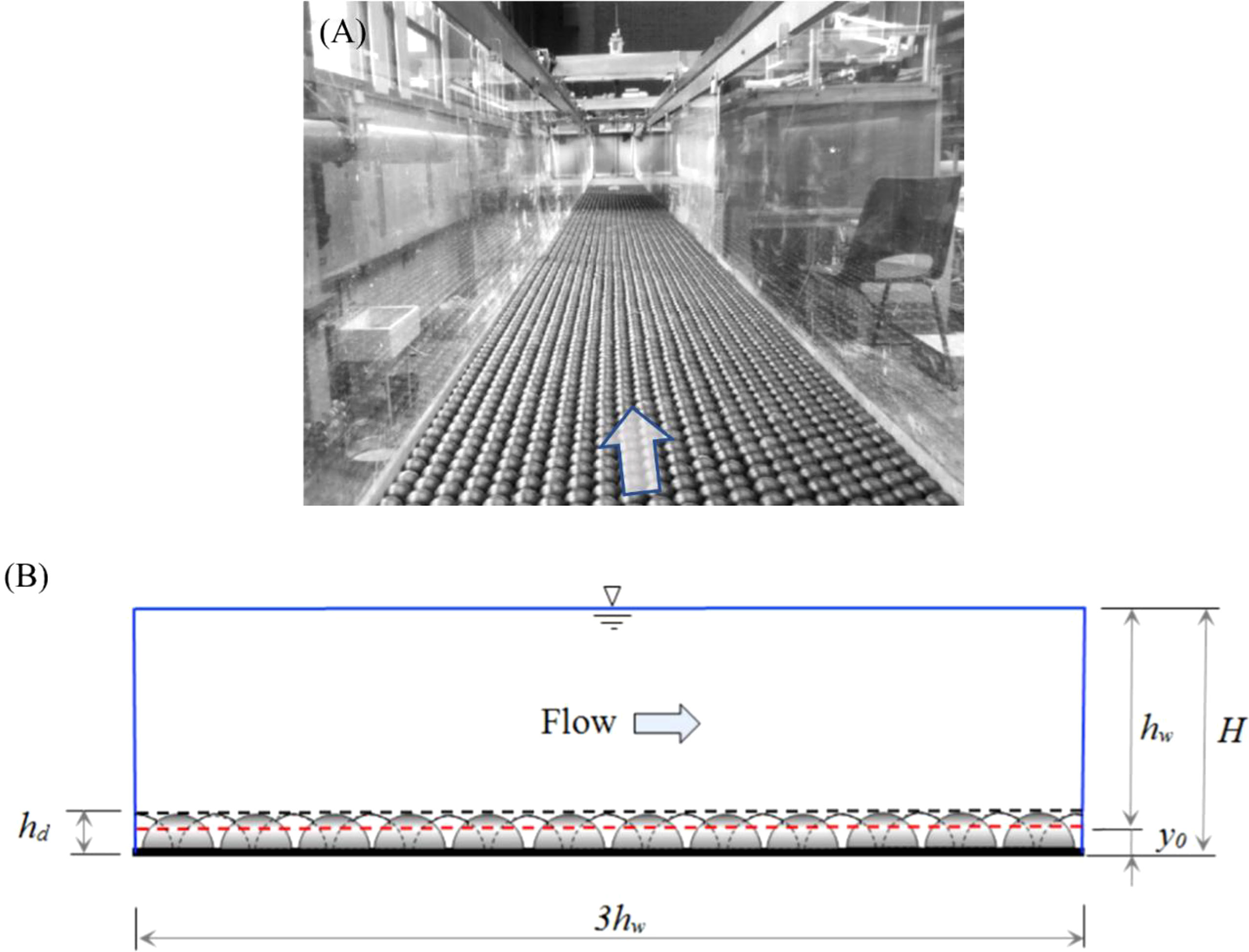
Figure 1 (A) Frontal view of the prototype flume and (B) longitudinal view through the centerline with rough bed spheres.

TABLE 1

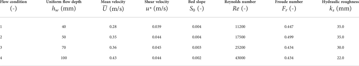
Table 1 Summary of the experimental flow conditions.

In Table 1, the shear velocity describes the gradient of velocity profile near the bed (< 20% of the total flow depth) and is calculated as $u^{\ast }=\sqrt{g{h}_w{S}_0}$. The Reynolds number Re is calculated by $\overline{U}{h}_w/{\upsilon }_0$ and Froude number by $F_r=\overline{U}/\sqrt{g{h}_w}$. The hydraulic roughness k_s is determined by fitting the average streamwise velocity profile measured in the centerline of the flume to the log-law for the rough bed turbulent flows. For each flow condition, the bed slope of the flume was controlled by using the adjustable jack located at the outlet end. The uniform flow depth h_w was measured by three-point gauges, located near the measurement sections at 4.5 m, 9.5 m, and 11.0 m measured from the flow inlet, respectively. The zero data were taken as the mean hemisphere elevation (4.0 mm below the top of the spheres), from which the uniform flow depth h_w was measured. Inside the measurement section, 3D side-looking acoustic Doppler velocimetry (ADV) probe was mounted on a scaled mechanical frame. This allowed the instrument to measure the flow velocity components in three different directions. The size of the sampling volume was 6 mm (diameter) and 6 mm (height), which was located 5 cm away from the tip of the ADV transmitter. The experiments were started by switching on the pump and carefully adjusting the flow rate by an adjustable valve located in the inlet pipe. The uniform flow was then established using the adjustable plate located at the flume outlet. The maximum deviation between the flow depths measured by the three-point gauges stayed below 1.5% of the mean flow depth. This indicates that the water surface slope was almost equal to the bed slope for the four flow conditions. The flow rate was determined by using a calibrated orifice plate located in the inlet pipe. For each flow condition, the flow was run at least 1 h before the measurements were taken. This allows the equilibrium conditions to be established.

The measurement section was located 9.5 m away from the inlet, which is believed to be sufficient to allow the stable flow condition to establish. Lateral profiles of the streamwise velocity and shear stress were measured for flow conditions 2 (shallow depth) and 4 (deep depth), whereas only vertical profiles of the streamwise and shear stress at the flume centerline were measured for flow conditions 1 (shallow depth) and 3 (deep depth). These measured data of flow velocity and shear stress are then used to validate the 3D SPH model results in the next section.

Smoothed particle hydrodynamics simulations and result analyses

This section introduces 3D SPH model validations with experimental data and the simulated flow patterns in the longitudinal and transverse directions. It shows the potential SPH applications in complex unilateral flows found in a coastal environment, such as the coastal current flows over a rough surface morphology.

Computational setup and model parameters

To be dimensionally consistent with the physical experiment, the width of numerical flume was taken 0.46-m wide for all the flow conditions. Considering sufficient numerical accuracy and low CPU load, the flume length was taken three times the flow depth. This length was believed to be sufficient to visualize the spatial patterns of secondary flow, bed shear stress and water surface. The initial particle size was selected to be 0.0015 m for flow conditions 1 and 2, and 0.0025 m for conditions 3 and 4, respectively. This provides 800,000–980,000 particles in the computation domain. The selection of particle size was to ensure enough resolution within the bed roughness elements and also minimize the kernel truncation errors near the solid boundaries. A cubic spline kernel was adopted with kernel size of h = 1.5 dx. The real water viscosity (υ₀ = 10⁻⁶ m²/s) was used and MLS filter was used every 30 time-steps to smooth out density and pressure fluctuations. The computational time step was automatically adjusted by following Courant stability requirement (Gomez-Gesteira et al., 2012). To reduce the CPU time and maintain the flow stability, a speed of sound c₀ = 20 m/s was used throughout the computations. This value is approximately three times larger than the minimum requirement.

The position of vertical origin (y = 0) at which the velocity is zero can be set at a distance of h_d below the top of the roughness sphere element. The value of h_d (roughness height) also represents the effective drag area to the flow and can be determined in such a way that the streamwise velocity distribution fit the log-law. In the experimental studies using hemispherical roughness elements of diameter D, slightly different values of h_d/D have been documented, being in the range of 0.15–0.35. To numerically investigate this issue, our SPH simulations were performed under four different values of h_d = 0.24 D, 0.28 D, 0.32 D, and 0.4 D, respectively, for each flow condition. By trial and errors, a value of roughness height h_d = 0.32 D was found to be applicable to flow conditions 1 and 2 (shallow depth) and h_d = 0.24 D, for the flow conditions 3 and 4 (deep depth). It is noted that these values are well within the previous experimental ranges. The values of h_d also make physical sense, since the shallow flows experience proportionally higher flow resistance and therefore the physical roughness elements generate larger numerical roughness height. It clearly shows that the roughness height h_d is a dynamic parameter, depending not only on the absolute value of the bed roughness size but also on the corresponding flow depth. More detailed discussions can be referred in the dissertation report (Gabreil, 2017). Besides, in our laboratory experiment, the flow velocity profile was measured from 4 mm below the crest of the rough sphere element, at which the mean flow depth h_w is defined. Therefore, we have h_d = y₀ + 4 mm, and we also use y₀ and h_w to normalize the vertical coordinate in the results. More details can be found in Gabreil (2017).

The SPH numerical model runs until the simulation time t exceeds 6.0 s. To reduce the time of simulation and to reach the stable flow conditions quicker, an analytical solution based on the power law U = U_max(y/H)^(1/m) was initially imposed within the fluid block for each flow condition. U_max is the maximum flow velocity in the streamwise velocity profile, which usually occurs at the free surface. The values of m take 2.8, 3.0, 3.2, and 3.8 for the flow conditions 1–4, respectively. It should be noted that nothing else has been imposed on the inflow/outflow conditions, channel bed and sidewall boundaries, rather the turbulent flows are naturally evolved by the influence of proposed 3D turbulence model and drag force equations. It was observed that the stable lateral bed shear stresses have been achieved at t = 3.0 s after the flows were initiated for all the four flow conditions. This was followed by further 3.0 s of data gathering without the influence of initial setup. It was also necessary to check the time convergence of the computed depth-averaged streamwise velocities $\overline{U}$ from t = 3.0 s -6.0 s, and the standard deviations for all test conditions were found to change within ±2.0%.

Flow patterns in the longitudinal direction

The spatial patterns of the time-averaged streamwise velocities in the longitudinal direction at the flume centerline were computed and plotted in Figures 2A–D for the four flow conditions 1, 2, 3, and 4 as shown in Table 1. These contour plots exhibit the smooth patterns that develop in almost parallel layers, which indicate that the fluid particle distributions are orderly without any persistent numerical noises in the particle field. Furthermore, the contour plots of the time-averaged pressures in the longitudinal direction presented in Figures 3A–D further reveal the smooth patterns such that they decrease almost linearly from the bed toward the free surface without significant numerical noises. Here, it should be noted that the dashed semi-circles on the bed seem not to be dimensionally uniform due to the normalization of different flow depths (shallow or deep conditions).

FIGURE 2

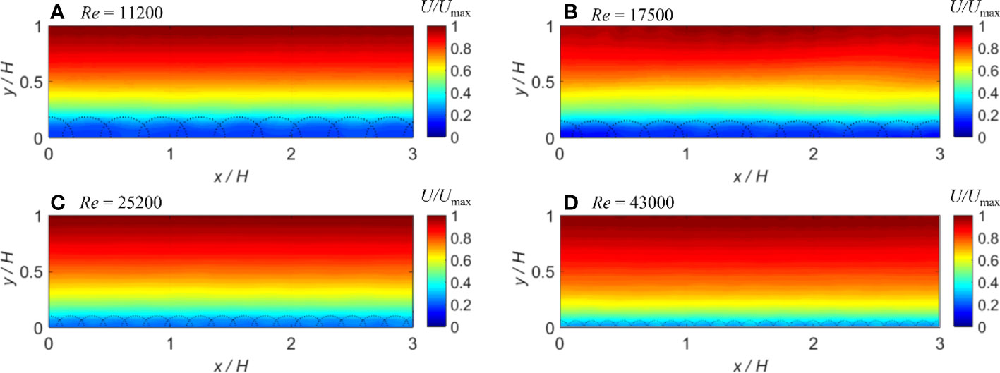
Figure 2 (A–D) Longitudinal contours of computed time-averaged streamwise velocities at the flume centerline for different flow conditions. The dashed semicircles at the bottom of each panel represent the rough bed spheres.

FIGURE 3

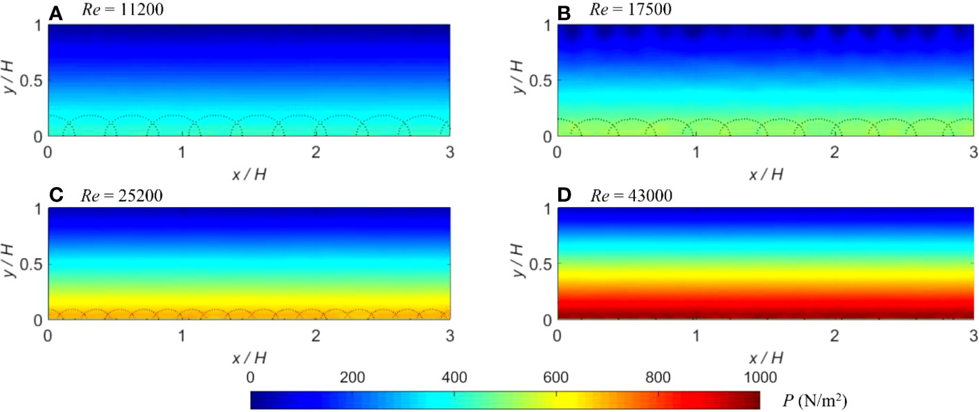
Figure 3 (A–D) Longitudinal contours of computed time-averaged pressures at the flume centerline for different flow conditions. The dashed semicircles at the bottom of each panel represent the rough bed spheres.

To validate SPH computations, Figures 4A–D present the comparisons of measured and computed time-averaged streamwise velocity profiles at the flume centerline for the four test conditions. The computed profiles were obtained by spatially averaging the contours shown in Figure 2. It is shown that the measured and computed profiles reveal a satisfactory agreement in the upper region of the flow, while the computed values were slightly under-predicted near the bed region for all the flow conditions. The averaged errors between experimental and numerical values were calculated to be 6.36%, 6.52%, 7.07%, and 7.51%, respectively, for each flow condition in Figure 4.

FIGURE 4

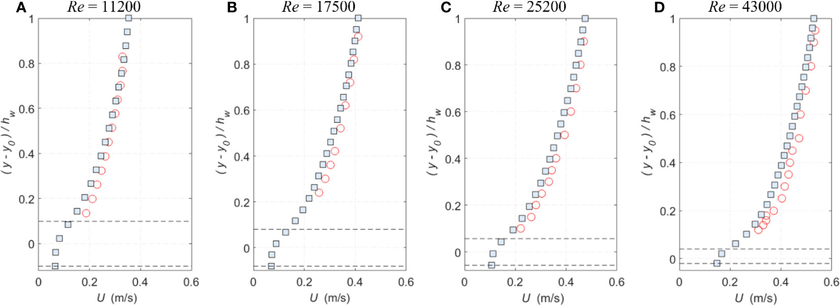
Figure 4 (A–D) Comparisons of time-averaged streamwise velocity profiles at the flume centerline for different flow conditions (circles: exp data; squares: smoothed particle hydrodynamics [SPH]; and dash lines: roughness top and bottom).

The spatial patterns of shear stress throughout the flow depths in Figures 5A–D demonstrate a gradual decreasing magnitude toward the free surface. The largest shear stress values occur on the top of the sphere, and these slightly vary in the streamwise direction. This spatial variation might be due to the secondary flows. Unlike previous 2D SPH simulations (Gabreil et al., 2018), a much better quantitative agreement between the computed, measured, and analytical shear stress profiles has been achieved in the present 3D model results, which is shown in Figures 6A–D. The averaged errors between experimental and numerical values were calculated to be 16.50%, 14.67%, 21.55%, and 10.76%, respectively, for each flow condition in Figure 6. It has been noted that flow condition 4 (the deepest depth with Re = 43,000) shows the largest deviation between the measured and predicted bed shear stress (16.0% of τ_b), where τ _b is the bed shear stress calculated from τ _b = ρg(H-h_d)S₀. This could be attributed to the measurement uncertainties, or the numerical conditions might still be in a non-uniform flow regime.

FIGURE 5

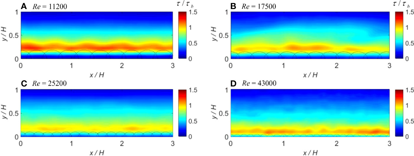
Figure 5 (A–D) Longitudinal contours of computed time-averaged shear stresses at the flume centerline for different flow conditions. The dashed semicircles at the bottom of each panel represent the rough bed spheres.

FIGURE 6

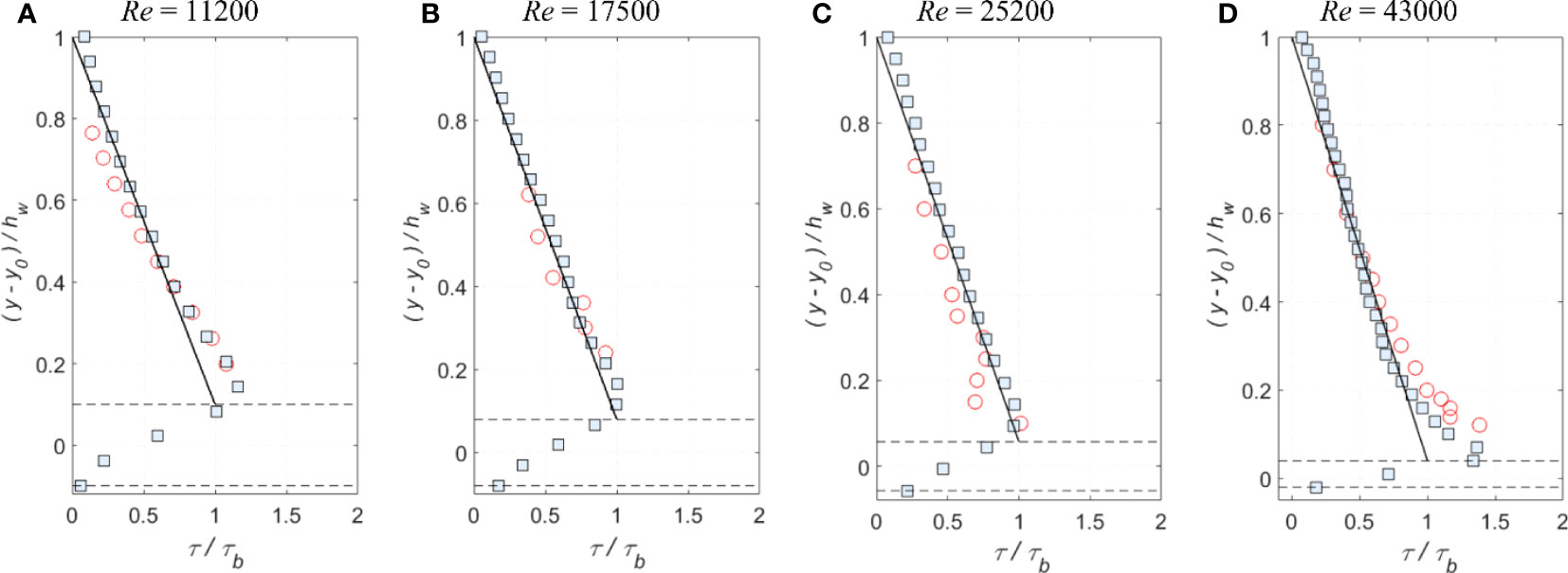
Figure 6 (A–D) Comparisons of time-averaged shear stress profiles at the flume centerline for different flow conditions (circles: exp data; squares: smoothed particle hydrodynamics [SPH]; solid black lines: analytical; and dash lines: roughness top and bottom).

Flow patterns in the lateral direction

The spatial patterns of hydrodynamic parameters over the flow cross section from the roughness bed to free surface are plotted in Figures 7–10 for the flow conditions 1–4, from shallow to deep flows, respectively. These results were obtained by averaging the flow fields over time t = 0.2 s. The averaging period was found to be sufficiently long to resolve the strongest secondary flows. The spatial averaging resolution used Δy = Δz = 0.0025 m for the flow conditions 1 and 2, and Δy = Δz = 0.005 m for the flow conditions 3 and 4. These resolutions depend on the original SPH particle spacing used for the computations, where two different values of 0.0015 m and 0.0225 m were used for the shallow and deep flow conditions, respectively. As for the spatial averaging resolutions Δy and Δz, they are usually selected to be 1.5–2 times of the particle spacing to ensure the elimination of particle fluctuations, and meanwhile, avoid over-smoothing of hydrodynamic variables in SPH post-data processing. The mean streamwise U, vertical V and lateral W velocities are all normalized by the maximum streamwise velocity U_max, whereas the shear stresses are all normalized by the bed shear stress calculated from τ _b = ρg(H-h_d)S_0. The experimental data are available for comparison for flow conditions of 2 (shallow depth) and 4 (deep depth). Here, it should be mentioned again that the dashed semi-circles on the bed seem not to be dimensionally uniform due to the normalization of different flow depths (shallow or deep conditions).

FIGURE 7

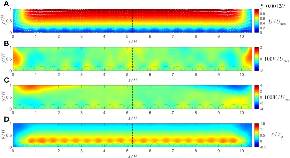
Figure 7 (A–D) Cross-sectional distributions of hydrodynamic parameters computed for flow condition 1 (shallow depth: Re = 11,200) including the roughness elements: normalized mean (A) streamwise velocity with vector field; (B) vertical velocity; (C) lateral velocity; and (D) shear stress. The dashed semicircles at the bottom of each panel represent the rough bed spheres.

FIGURE 8

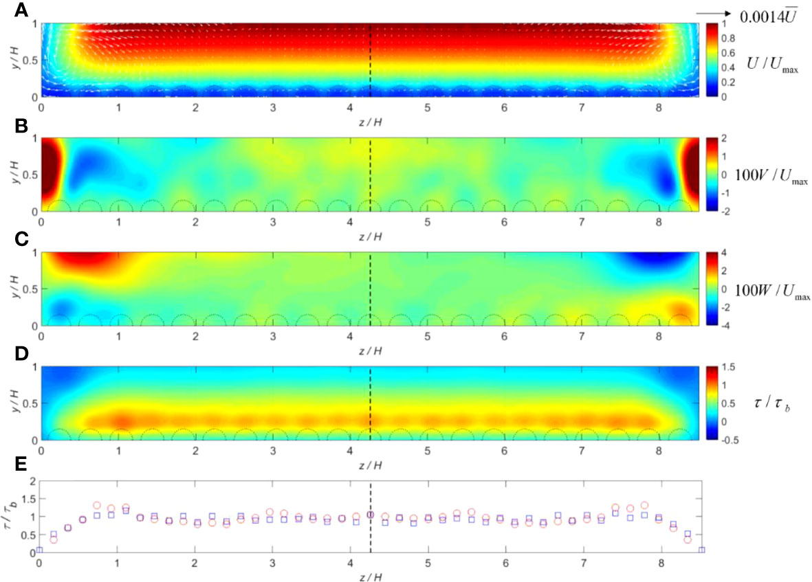
Figure 8 (A–E) Cross-sectional distributions of hydrodynamic parameters computed for flow condition 2 (shallow depth: Re = 17,500) including the roughness elements: normalized mean (A) streamwise velocity with vector field; (B) vertical velocity; (C) lateral velocity; (D) shear stress; and (E) measured and computed bed shear stress (circles: exp data; squares: SPH). The dashed semicircles at the bottom of each panel represent the rough bed spheres.

FIGURE 9

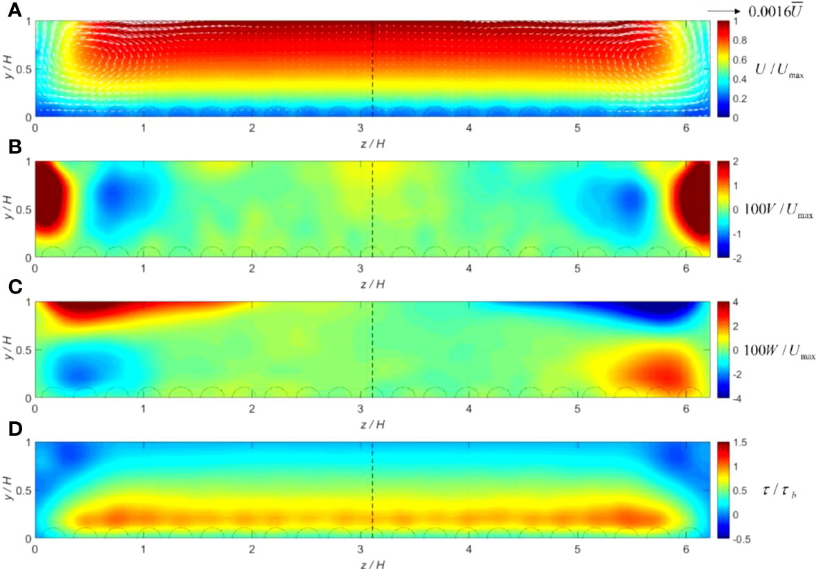
Figure 9 (A–D) Cross-sectional distributions of hydrodynamic parameters computed for flow condition 3 (deep depth: Re = 25,200) including the roughness elements: normalized mean (A) streamwise velocity with vector field; (B) vertical velocity; (C) lateral velocity; and (D) shear stress. The dashed semicircles at the bottom of each panel represent the rough bed spheres.

FIGURE 10

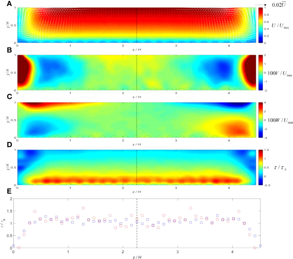
Figure 10 (A–E) Cross-sectional distributions of hydrodynamic parameters computed for flow condition 4 (deep depth: Re = 43,000) including the roughness elements: normalized mean (A) streamwise velocity with vector field; (B) vertical velocity; (C) lateral velocity; (D) shear stress; and (E) measured and computed bed shear stress (circles: exp data; squares: SPH). The dashed semicircles at the bottom of each panel represent the rough bed spheres.

From Figures 7–10, it is shown that the secondary flows develop throughout the whole width of the cross-sectional area, and they are also scaled with the flow depth. The rotational features of these currents are correlated with the patterns of vertical (V) and lateral (W) velocities. Regions of the up-flow (V > 0) and down-flow (V < 0) are approximately separated by a distance of 0.9H-1.2H in the lateral direction. The velocity vector fields show that the strongest flow cells occur near each side of the boundaries, which should transport high flow momentums from the free surface toward the channel bed, and thus cause the streamwise velocity to slightly bulge toward the sidewall corner. For flow conditions 1 and 2 (shallow depth), the secondary flows become weaker in the region away from the sidewalls. With the flow depth becoming deeper, such as in conditions 3 and 4, the secondary flow velocities also become larger. On the other hand, the cross-sectional distributions of computed shear stresses reveal a maximum value on the top of the roughness elements (where the streamwise velocity gradient dU/dy is largest), with a gradual decrease toward the free surface and sidewalls. Negative shear stresses are also observed in the small regions just below the water surface and next to the sidewalls, which may indicate a strong secondary flow cell.

In Figures 8E and 10E, to validate SPH simulation results, the lateral distributions of measured and computed bed shear stresses for flow conditions 2 (shallow depth) and 4 (deep depth) are compared respectively. The comparisons show a satisfactory agreement, and both the experimental and numerical shear stresses increase from the minimum value on sidewalls to a peak in the flume center, which is 30%–50% larger than τ_b. The averaged errors were found to be 12.33% and 14.35%, respectively, for Figures 8E and 10E.

To further evaluate the accuracy of proposed 3D SPH model results, the lateral profiles of time-averaged streamwise velocity and shear stress in the up-flow (V > 0) and down-flow (V < 0) zones were compared with the experimental data for flow condition 2 (shallow depth) in Figures 11, 12A–E, and flow condition 4 (deep depth) in Figures 13, 14A–C, respectively.

FIGURE 11

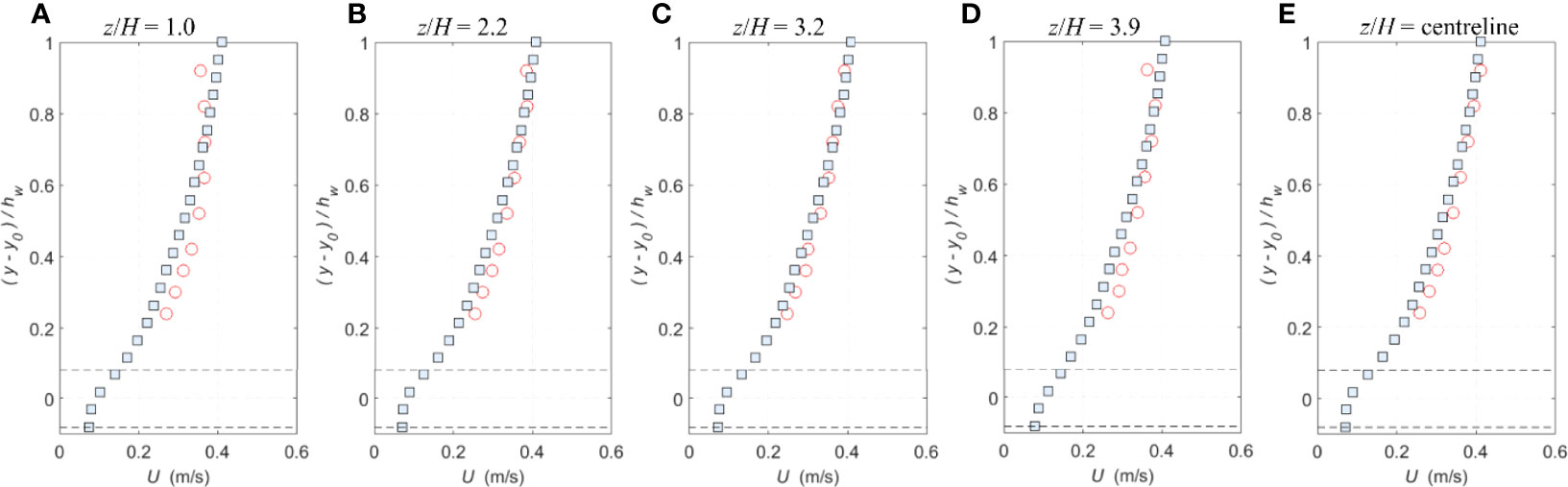
Figure 11 (A–E) Comparisons of the lateral profiles of time-averaged streamwise velocity between experimental and SPH results for shallow flow condition 2 (circles: exp data; squares: SPH; and dash lines: roughness top and bottom).

FIGURE 12

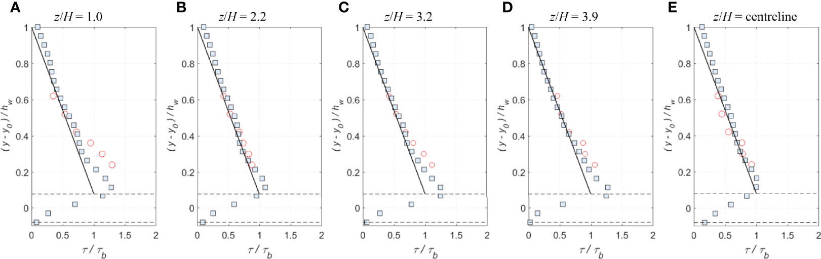
Figure 12 (A–E) Comparisons of the lateral profiles of time-averaged shear stress between experimental, analytical and SPH results for shallow flow condition 2 (circles: exp data; squares: SPH; solid black lines: analytical; and dash lines: roughness top and bottom).

FIGURE 13

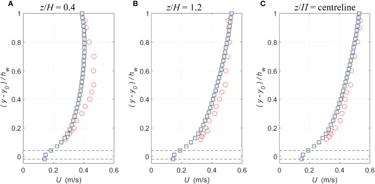
Figure 13 (A–C) Comparisons of the lateral profiles of time-averaged streamwise velocity between experimental and SPH results for deep flow condition 4 (circles: exp data; squares: SPH; and dash lines: roughness top and bottom).

FIGURE 14

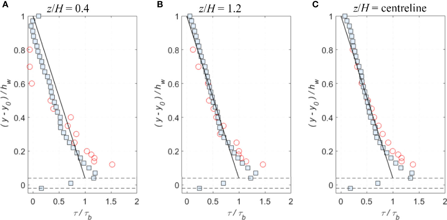
Figure 14 (A–C) Comparisons of the lateral profiles of time-averaged shear stress between experimental, analytical and SPH results for deep flow condition 4 (circles: exp data; squares: SPH; solid black lines: analytical; and dash lines: roughness top and bottom).

In Figures 11A–E, the SPH results slightly under-predict the time-averaged streamwise velocities for all the compared profiles. In the upper flow region (y-y₀)/h_w > 0.6, the largest error in U occurs in the lateral profile close to the sidewall (z/H = 1) reaching approximately 2.0%. This might be due to the difficulty in simulating the velocity dip in this shallow condition (2), whereas the experimental velocity profile clearly indicates the existence of a velocity dip. In Figures 12A–E, the SPH shear stress profiles are generally consistent with the measured and analytical ones. Again, there appears a large disagreement close to the sidewall (z/H = 1), which was found to be approximately 22.0% of τ_b. The discrepancy could be due to the physical velocity dip as mentioned before, or due to the numerical treatment of roughness elements on sidewalls.

Besides, Figures 13A–C shows the lateral profiles of measured and computed time-averaged streamwise velocities for flow condition 4 (deep depth). Once again, close to the sidewall at z/H = 0.4, the computed velocity profile is smaller than the measurement around 0.3 < (y-y₀)/h_w < 0.8, in spite that both profiles agree well in the near bed and water surface. An error analysis showed a maximum error of 3.0% in the middle region of the flow. This could be attributed to the fact that the computed secondary flow is not strong enough to bulge the streamwise velocity as observed in the experimental measurement. On the other hand, the corresponding shear stress profiles in Figures 14A–C also indicate the maximum deviation occurring somewhere to the sidewall (z/H = 0.4), which is about 26.0% of τ _b. It is also worth noting that the measured and computed shear stress values here are smaller than the analytical solutions in the upper flow region (y-y₀)/h_w > 0.25, and this might be attributed to the secondary flows that move from the free surface toward the bed. The measured shear stresses approach to zero from (y-y₀)/h_w ≥ 0.6, while the computed ones demonstrate this trend only from 0.85. This is a clear sign that the computed secondary flows are weaker than the observed ones in the laboratory experiment.

Conclusions

This study developed a 3D numerical model based on the SPH approach that could be used to predict the flow velocity and shear stress distributions in practical turbulent unilateral flows over a fixed rough bed surface, such as the near-shore flow currents approaching the coastal region. To validate the numerical results, experimental measurements of the flow velocity and shear stress were carried out for a wide range of flow conditions with different Froude and Reynolds numbers. The numerical program is based on the open-source code 3D SPHysics. Model improvements were made on the turbulence closure, and rough bed and sidewall treatment. Then a modified SPS mixing length model is proposed, with an improved drag force equation acting in the streamwise, vertical and lateral directions being included in the momentum equations.

The proposed 3D SPH model is shown capable of reproducing a stable secondary flow pattern across the flow area for different flow conditions. The lateral distributions of shear stresses have been validated against the experimental data with a mean square error of 4.0%, despite the maximum errors near the sidewall can reach as large as 25%. On the other hand, the comparisons between measured and computed profiles of streamwise velocity and shear stress at the flume centerline are also in satisfactory agreement. This is manifested by the fact that the average velocity errors are around 7.5% and average shear stress errors are around 15% for most flow conditions.

It should be mentioned that the numerical findings in this paper are not an indication that the pioneering benchmark SPS turbulence model (Gotoh et al., 2001) with a fixed Smagorinsky constant cannot always provide the correct shear flow mechanisms. The present rough bed could cause flow dispersion throughout the whole depth, and as a result, more realistic shear stress values should be reproduced if a more refined computational particle resolution is used.

Data availability statement

The raw data supporting the conclusions of this article will be made available by the authors, without undue reservation.

Author contributions

EG: methodology, simulation, visualization, validation, analysis, and writing—original draft. HW: investigation and writing—review and editing. CC: investigation and writing—review and editing. JL: investigation and writing—review and editing. MR: investigation and writing—review and editing. XZ: investigation and writing—review and editing. SS: supervision, conceptualization, management, and writing—review and editing. All authors contributed to the article and approved the submitted version.

Funding

This research work is supported by the National Natural Science Foundation of China (no. 51879051), Key Funded Disciplinary Research Promotion Project of Guangdong Higher Education Institutes (no. 226115001023), Major Project of Qinghai Provincial Department of Science and Technology (no. 2021-SF-A6) and GuanDong Basic and Applied Basic Research Foundation (no. 2021A1515110768).

Acknowledgments

The first and last authors acknowledge the support of Professor Simon Tait at The University of Sheffield for jointly supervising the research project. We all acknowledge the Frontier Editorial Team and Editor Professor Riccardo Briganti for their professional handling of the manuscript and two dedicated referees who provided very constructive and insightful comments to significantly improve the quality of the work. Author Songdong Shao also appreciates the useful feedbacks from Professor Pengzhi Lin of Sichuan University during the revision of the manuscript.

Conflict of interest

The authors declare that the research was conducted in the absence of any commercial or financial relationships that could be construed as a potential conflict of interest.

Publisher’s note

All claims expressed in this article are solely those of the authors and do not necessarily represent those of their affiliated organizations, or those of the publisher, the editors and the reviewers. Any product that may be evaluated in this article, or claim that may be made by its manufacturer, is not guaranteed or endorsed by the publisher.

References

Altomare C., Gironella X., Crespo A. J. C. (2021). Simulation of random wave overtopping by a WCSPH model. Appl. Ocean Res. 116, 102888. doi: 10.1016/j.apor.2021.102888

CrossRef Full Text | Google Scholar

Bartzke G., Fourtakas G., Canelas R., Rogers B. D., Huhn K. (2021). Simulation of flow past a sphere on a rough bed using smoothed particle hydrodynamics (SPH). Comput. Particle Mechanics. doi: 10.1007/s40571-021-00417-x

CrossRef Full Text | Google Scholar

Brakenhoff L., Schrijvershof R., van der Werf J., Grasmeijer B., Ruessink G., van der Vegt M. (2020). From ripples to large-scale sand transport: The effects of bedform-related roughness on hydrodynamics and sediment transport patterns in Delft3D. J. Mar. Sci. Eng. 8, 892. doi: 10.3390/jmse8110892

CrossRef Full Text | Google Scholar

Chen H., Tsai C. (2012). Computations of nearshore wave transformation using finite-volume method. Appl. Ocean Res. 38, 32–39. doi: 10.1016/j.apor.2012.07.001

CrossRef Full Text | Google Scholar

Czernuszenko W., Rylov A. A. (2000). A generalisation of prandtl’s model for 3D open channel flows. J. Hydraulic Res. 38, 173–180. doi: 10.1080/00221680009498335

CrossRef Full Text | Google Scholar

Dalrymple R. A., Knio O. (2001). “SPH modelling of water waves,” in Proceedings of 4th International Conference on Coastal Dynamics, , June. 779–787.

Google Scholar

De Padova D., Mossa M., Sibilla S., Torti E. (2013). 3D SPH modelling of hydraulic jump in a very large channel. J. Hydraulic Res. 51, 158–173. doi: 10.1080/00221686.2012.736883

CrossRef Full Text | Google Scholar

Duan G., Chen B. (2015). Large Eddy simulation by particle method coupled with Sub-Particle-Scale model and application to mixing layer flow. Appl. Math. Model. 39, 3135–3149. doi: 10.1016/j.apm.2014.10.058

CrossRef Full Text | Google Scholar

Džebo E., Žagar D., Krzyk M., Četina M., Petkovšek G. (2014). Different ways of defining wall shear in smoothed particle hydrodynamics simulations of a dam-break wave. J. Hydraulic Res. 52, 453–464. doi: 10.1080/00221686.2013.879611

CrossRef Full Text | Google Scholar

Farahani R. J., Dalrymple R. A., Hérault A., Bilotta G. (2012). SPH modeling of mean velocity circulation in a rip current system. 3rd Int. Conf. Coast. Eng. doi: 10.9753/icce.v33.currents.37

CrossRef Full Text | Google Scholar

Fedderico I., Marrone S., Colagrossi A., Aristodemo F., Antuono M. (2012). Simulating 2D open-channel flows through an SPH model. J. Hydraulic Res. 34, 35–46. doi: 10.1016/j.euromechflu.2012.02.002

CrossRef Full Text | Google Scholar

Gabreil E. (2017). Application of smoothed particle hydrodynamics modelling to turbulent open channel flows over rough beds (Sheffield, UK: University of Sheffield).

Google Scholar

Gabreil E., Tait S. J., Shao S., Nichols A. (2018). SPHysics simulation of laboratory shallow free surface turbulent flows over a rough bed. J. Hydraulic Res. 56, 727–747. doi: 10.1080/00221686.2017.1410732

CrossRef Full Text | Google Scholar

Gomez-Gesteira M., Rogers B. D., Crespo A. J. C., Dalrymple R. A., Narayanaswamy M., Dominguez J. M. (2012). SPHysics - development of a free-surface fluid solver - part 1: Theory and formulations. Comput. Geosciences 48, 289–299. doi: 10.1016/j.cageo.2012.02.029

CrossRef Full Text | Google Scholar

Gotoh H., Shibahara T., Sakai T. (2001). Sub-Particle-Scale turbulence model for the MPS method — Lagrangian flow model for hydraulic engineering. J. Comput. Fluid Dynamics 9, 339–347.

Google Scholar

Gu S., Zheng W., Wu H., Chen C., Shao S. (2022). DualSPHysics simulations of spillway hydraulics: a comparison between single- and two-phase modelling approaches. J. Hydraulic Res. doi: 10.1080/00221686.2022.2064343

CrossRef Full Text | Google Scholar

Harris L., Liang D., Shao S., Zhang T., Roberts G. (2021). MPM simulation of solitary wave run-up on permeable boundaries. Appl. Ocean Res. 111, 102602. doi: 10.1016/j.apor.2021.102602

CrossRef Full Text | Google Scholar

Kazemi E., Koll K., Tait S., Shao S. (2020). SPH modelling of turbulent open channel flow over and within natural gravel beds with rough interfacial boundaries. Adv. Water Resour. 140, 103557. doi: 10.1016/j.advwatres.2020.103557

CrossRef Full Text | Google Scholar

Lowe R. J., Buckley M. L., Altomare C., Rijnsdorp D. P., Suzuki T., Bricker J. (2019). “Improving predictions of nearshore wave dynamics and coastal impacts using smooth particle hydrodynamic models,” in 2019 Australasian Coasts and Ports Conference, , September.

Google Scholar

Meister M., Burger G., Rauch R. (2014). On the reynolds number sensitivity of smoothed particle hydrodynamics. J. Hydraulic Res. 52, 824–835. doi: 10.1080/00221686.2014.932855

CrossRef Full Text | Google Scholar

Monaghan J. J. (1994). Simulating free surface flows with SPH. J. Comput. Phys. 110, 399–406. doi: 10.1006/jcph.1994.1034

CrossRef Full Text | Google Scholar

Nam P. T., Larson M., Hanson H., Hoan L. (2009). A numerical model of nearshore waves, currents, and sediment transport. Coast. Eng. 56, 1084–1096. doi: 10.1016/j.coastaleng.2009.06.007

CrossRef Full Text | Google Scholar

Ruffini G., Briganti R., De Girolamo P., Stolle J., Ghiassi B., Castellino M. (2021). Numerical modelling of flow-debris interaction during extreme hydrodynamic events with DualSPHysics – CHRONO. Appl. Sci. 11, 3618. doi: 10.3390/app11083618

CrossRef Full Text | Google Scholar

Tang J., Lyu Y., Shen Y., Zhang M., Su M. (2017). Numerical study on influences of breakwater layout on coastal waves, wave-induced currents, sediment transport and beach morphological evolution. Ocean Eng. 141, 375–387. doi: 10.1016/j.oceaneng.2017.06.042

CrossRef Full Text | Google Scholar

Violeau D., Issa R. (2007). Numerical modelling of complex turbulent free surface flows with the SPH method: An overview. Int. J. Numerical Methods Fluids 53, 277–304. doi: 10.1002/fld.1292

CrossRef Full Text | Google Scholar

Wang D., Liu P. L.-F. (2020). An ISPH with k–ϵ closure for simulating turbulence under solitary waves. Coast. Eng. 157, 1–28. doi: 10.1016/j.coastaleng.2020.103657

CrossRef Full Text | Google Scholar

Yang S., Lim S. (1997). Mechanism of energy transportation and turbulent flow in a 3D channel. J. Hydraulic Eng. 123, 684–692. doi: 10.1061/(ASCE)0733-9429(1997)123:8(684)

CrossRef Full Text | Google Scholar

Yao Y., Chen X., Xu C., Jia M., Jiang C. (2022). Numerical modelling of wave transformation and runup over rough fringing reefs using VARANS equations. Appl. Ocean Res. 118, 102952. doi: 10.1016/j.apor.2021.102952

CrossRef Full Text | Google Scholar

Zhang J., Larson M., Ge Z. (2020). Numerical model of beach profile evolution in the nearshore. J. Coast. Res. 36, 506–520. doi: 10.2112/JCOASTRES-D-19-00065.1

CrossRef Full Text | Google Scholar

Appendix convergence analysis

This appendix checks the convergence of SPH computation in spatial domain using two different particle sizes for the flow conditions of Re = 11,200 and 25,200, representing the shallow and deep flow depths, respectively. Figures A1A, B show the computed time-averaged streamwise velocity at dx = 1.5 mm (original run) and 2.0 mm (new run) for the flow condition of Re = 11,200, and dx = 2.5 mm (original run) and 3.0 mm (new run) for the flow condition of Re = 25,200, while Figures A1C, D present the computed shear stresses correspondingly. The selection of these particle resolutions aimed to ensure at least 20 particles exist in the depth direction of flow to satisfy the numerical accuracy.

FIGURE A1

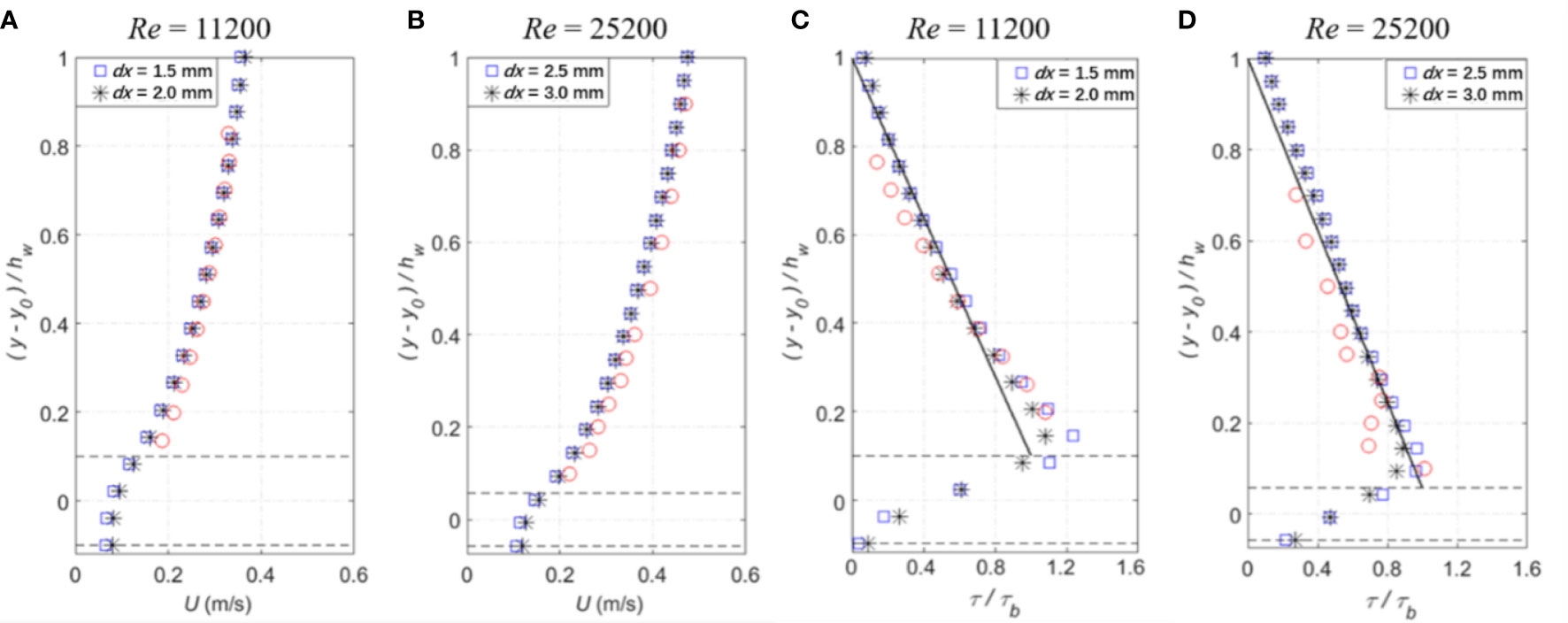
Figure A1 (A–D) Convergence studies: Comparisons between experimental (red circles), (A, B) SPH velocity profiles, and (C, D) SPH and analytical (black solid line) shear stress profiles, at two different particle resolutions for shallow and deep flow conditions.

Figures A1A–D reveal a good overlapping behavior along the flow depth for the two different particle sizes, indicating the convergence of numerical results. However, when the larger particle size is used for the two different flow conditions, the shear stress values decrease by as large as 10% of τ_b in the area just above the roughness top. This indicates that a more demanding spatial resolution of particles should be used near the roughness interface to obtain accurate velocity gradient there.