Hurricane and Typhoon Storm Wind Resolving NOAA NCEI Blended Sea Surface Wind (NBS) Product

1 Introduction

Surface wind is an essential climate variable. It drives the exchange of momentum between the atmosphere and ocean, generates ocean waves, and acts as a driving force for the ocean circulations responsible for the global transport of important properties such as momentum/energy, heat, and carbon. Extreme winds have huge social and economic impacts, most obviously during hurricanes and tropical cyclones (TCs), leading to loss of human life, damage to ecosystems, and destruction of properties and infrastructure. Two of the major extreme weather events related to winds are TCs/hurricanes and extratropical bomb cyclones (ECs). To improve forecasting and analysis of such extreme events, better and more accurate observing systems are needed (Domingues et al., 2019), such as in situ measurements from ships, buoys, surface drifters, and satellite-based remote sensing consisting of observations from scatterometers, radiometers, reflectometers, and altimeters, etc. (Villas Bôas et al., 2019).

The advantage of satellite-derived winds compared to other sources is their vast spatial coverage at higher global spatial resolution. However, all observations have data gaps and also have inherent inaccuracies due to the errors associated with spacecraft navigation, sensor calibration and noise, retrieval algorithm limitations, etc. Over the past few decades, the oceanographic community has been trying to overcome the space and time gaps and heterogeneity by combining observations from multiple sensors. In this context, several multiple-sensor blended wind products are developed by the community. These include the Copernicus Marine Environment Monitoring Service (CMEMS) Global Blended Mean Wind Fields (Desbiolles et al., 2017), Cross-Calibrated Multi-Platform (CCMP) wind analysis (Atlas et al., 2011), and Ocean Surface Current Analysis Real-time (OSCAR, Bonjean and Lagerloef, 2002). All these products are blended, but gaps (either spatial or temporal) in measurements of winds, currents, and waves still remain. Also, none of these products are capable of delineating very high winds associated with extreme events like TCs and ECs.

The U.S. National Oceanic and Atmospheric Administration (NOAA) National Centers for Environmental Information (NCEI) Blended Sea winds (NBS) product is an important element in NOAA’s Blue Economy Strategic Plan, supporting mission areas in offshore renewable energy (wind farms), marine transportation, marine ecosystem and fisheries, and others. The previous version (v1.0) of NBS (Zhang et al., 2006) was developed using multiple sources to fill data gaps and reduce errors and aliases associated with the sub-sampling by the individual satellite observations. Taking advantage of multiple satellite sources and using wind directions from model reanalysis, blended sea surface (10 m neutral) vector winds had been generated on a global 0.25° regular grid for several time resolutions: 6-hourly, daily, monthly, as well as a long-term climatology (1995–2005). A simple objective analysis method, namely, a spatial-temporally weighted interpolation, is used to generate the 6-hourly blended product from multiple satellites. In particular, the formula by Zeng and Levy (1995) that was used to address time and space aliases in monthly mean scatterometer winds was used. However, the blended wind generated by this process was unable to delineate the very high winds especially in and around hurricanes and TCs. Our recent investigation shows that when such simple spatial–temporal averaging is used in the existing multi-satellite blending schedule, we noticed cases of either underestimating the strong storm peak winds or artifacts due to fast-moving storms. The underestimates were due to the fact that the majority of the input satellite data cannot resolve strong storm winds; thus strong winds are dampened in multi-satellite data blending.

To address the above shortcomings in the NBS with a capability to resolve storm winds in the multi-satellite blended product, a new version, NBS v2.0, is developed. This is achieved by adding a random-error based weighted averaging on top of the simple spatial–temporal weighted interpolation (similar to the previous version), as detailed below in Section 3. The rest of the paper is organized as follows: Section 2 describes the data used in NBS v2.0. Section 3 describes the blending techniques, which include both the objective analysis spatial–temporal weighting method and the random-error based weighting method. Section 4 details the implementation of the new blending techniques and development of NBS v2.0. Section 5 describes examples of high wind characterization during some TCs and hurricane events. Finally, Section 6 provides some concluding summaries and discussions.

2 Dataset used

The Remote Sensing Systems, Inc. (RSS) has been processing climate research quality satellite ocean winds (at 10-m height above sea level) from various satellite instruments from the late 1980s to present-day satellites. These include wind data from the Defense Meteorological Satellite Program (DMSP) Special Sensor Microwave/Imager (SSM/I) version 7 (Wentz et al., 2012), the Tropical Rainfall Measuring Mission (TRMM) Microwave Imager (TMI) version 7.1 (Wentz et al., 2015a), the Quick Scatterometer (QuikSCAT) version 4 (Ricciardulli et al., 2011), the Advanced Microwave Scanning Radiometer—EOS (AMSR-E) version 7 (Wentz et al., 2014a), AMSR-2 version 8.2 (Wentz et al., 2014b; Meissner et al., 2021), Advanced Scatterometer (ASCAT) version 2.1 (Ricciardulli and Wentz, 2016), WindSat polarimetric radiometer data version 7.0.1 (Wentz et al., 2013), Global Precipitation Measurement (GPM) Microwave Imager (GMI) version 8.2 (Wentz et al., 2015b), and Soil Moisture Active Passive (SMAP) version 1.0 (Meissner et al., 2018). Figure 1 shows the timeline of the satellite data from RSS used in our blended product.

FIGURE 1

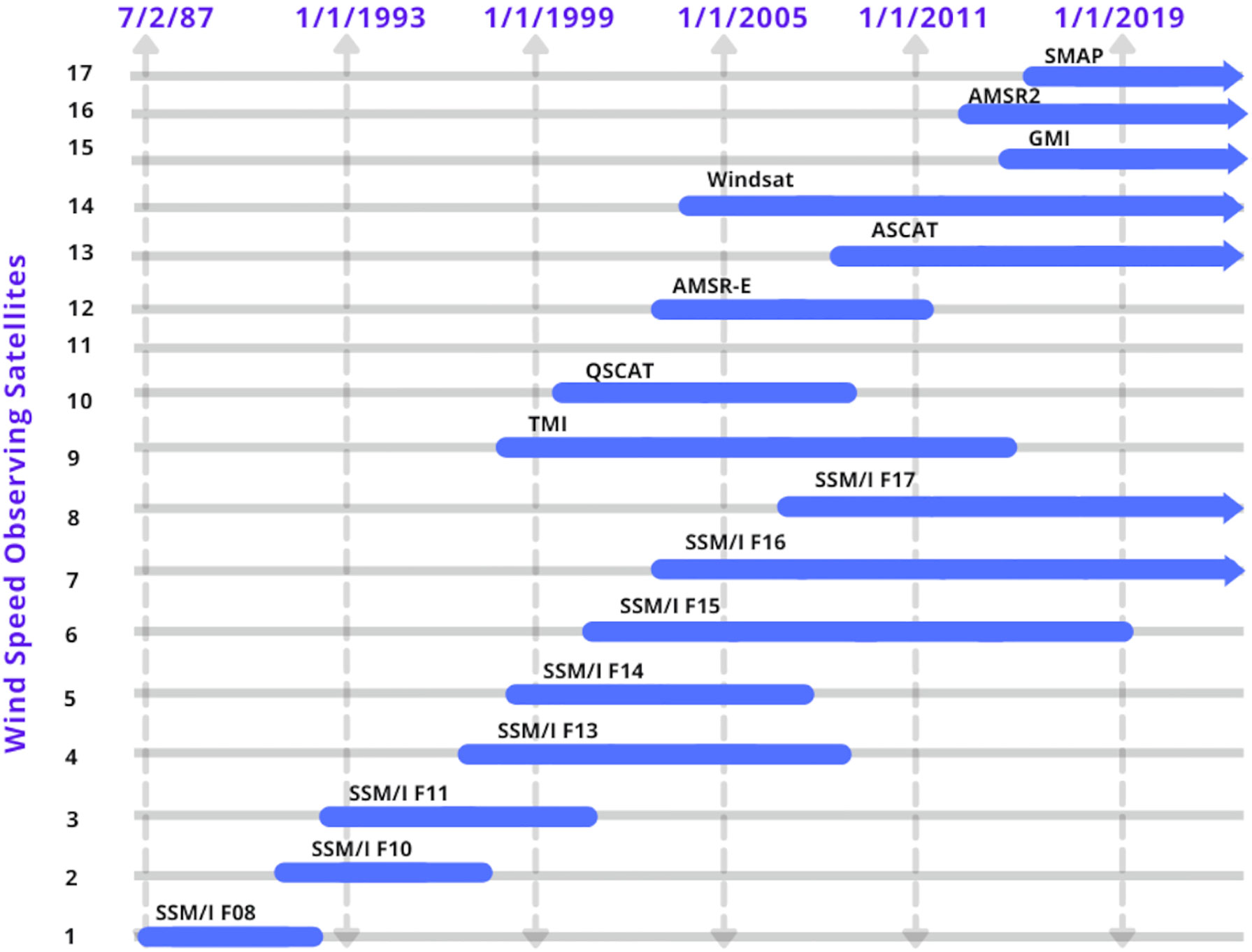
Figure 1 The primary U.S. wind speed observing satellites. Observations from these satellites are used to produce NBS products. The arrow represents data that are currently available into the future in near-real-time.

Throughout our processing that goes back to 1987, we used wind data derived from the 17 sensors. We downloaded the latest versions of the RSS satellite products at our processing time. RSS also operationally generates datasets in near-real-time (NRT) (with a latency of 1 day, with fewer quality controls), followed by delayed-mode final processing data (with latencies of minimum 2 days or longer), with better quality-controlled data (science quality) for a few of these sensors. Both the ascending and descending satellite swath data (representing morning and evening tracks) with a 0.25° resolution are used as input to our NBS product. Most of the imaging sensors/radiometers derive wind using 18.7- to 37-GHz channels (in medium frequencies) and ~11-GHz channels (in lower frequencies). For the TMI, data from both the 11 and 37 GHz channels are used. The new version of AMSR2 (version 8.2 recently released in May 2021 as a major update) has an extra all-weather channel in C-band (~6.9 GHz), which is rich with information about wind speeds in and around storms, including TCs.

The RSS data we used also include the L-band radiometers (~1.4 GHz) based on the wind from SMAP (Entekhabi et al., 2014), which is useful for the retrieval of high wind speeds around storms with heavy rain (Reul et al., 2012). Meissner et al., 2021 have detailed the TC wind speed algorithm that uses the wind speeds retrieved from SMAP (in L-band) and a combination of C and X band channels for TC-wind retrievals with reduced sensitivity to rain. This combination of C-band and X-band channels used for AMSR2 and WindSat is sensitive to wind speeds but insensitive to rain, thus reducing rain contamination. We also used the RSS scatterometer wind data, which were derived from the C-band (ASCAT) and Ku-band (QuikScat) with multiple polarization.

3 Blending techniques

3.1 Spatial–Temporal Weighted Interpolation

In the first step, a simple objective analysis method, namely, a three-dimensional spatial–temporal weighted interpolator (Zeng and Levy, 1995) that uses both spatial and temporal sampling patterns of satellite observation, is used to generate the 6-hourly and 0.25° grid blended product from multiple satellite observations. For the value at the grid location (x₀ , y₀ , and t₀) , this process searches for all available data values within horizontal range R and a temporal range of T. The value at (x₀ , y₀ , and t₀) is then estimated using linear weighted averaging for N observed values, as follows:

$\begin{array}{ll}{u}_{est}=\frac{{\sum }_{k=1}^N{w}_k{u}_k}{{\sum }_{k=1}^N{w}_k}& (1)\end{array}$

where uk is observational data at (xk , yk , and tk) and wk is a weighting function, derived as follows:

$\begin{array}{ll}{w}_k=\frac{2-\left[\frac{{\left(x_k-x_0\right)}^2+{\left(y_k-y_0\right)}^2}{R^2}+\frac{{\left(t_k-t_0\right)}^2}{T^2}\right]}{2+\left[\frac{{\left(x_k-x_0\right)}^2+{\left(y_k-y_0\right)}^2}{R^2}+\frac{{\left(t_k-t_0\right)}^2}{T^2}\right]}& (2)\end{array}$

In the above, x_k , y_k , and t_k are the location and time of the satellite data within the spatial range of R and temporal range of T. The averaging weights w_k are determined by the normalized “distances” (squared) in both space and time from the data points (denoted by subscript k) to the grid interpolation point (denoted by subscript 0). The R and T are the data averaging window sizes in space and time, respectively, chosen to be 62.5 km and 3 h from each side of the interpolation point for the 6-hourly products. The spatial window was chosen to avoid excessive smoothing of the blended output while having enough data to fill in the gridded points (Zhang et al, 2006).

The spatial–temporal component of the weighting function, w_k , has Gaussian characteristics (Figure 2), which plateaus near the center lag time. To the right of the center lag time, the weight function decreases slowly at first, followed by a rapid fall. The Gaussian profile ensures that far-field data contribute much less when nearby data are available.

FIGURE 2

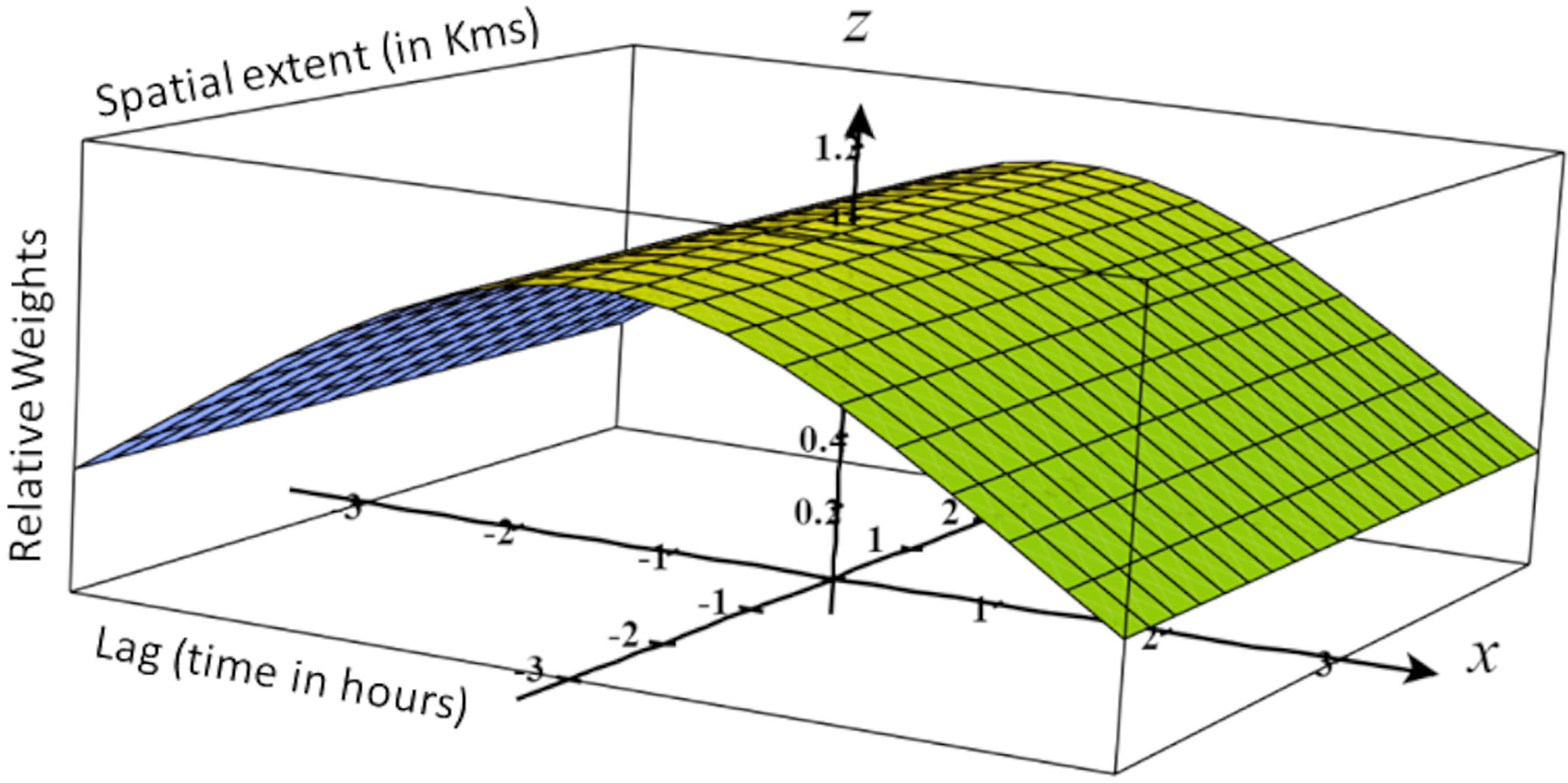
Figure 2 The interpolation weight function in the space–time domain w_k.

The multi-satellite blended global gridded winds are generated on a 0.25° global grid with a 6-hourly time resolution at 0000, 0600, 1200, and 1800 UTC grid points. For the 0000 UTC center time, 3 h of data from the previous day (2100 to 2400 UTC) are used. Note that the time grid points are in UTC and should not be interpreted as “morning/evening” time in the sense of local solar time. The final output is a 0.25° in the spatial grid between the longitude 0° to 359.75°E and 89.75°S to 89.75°N in latitude. The resulting grid points are mostly filled by blending satellite observations as above, but some gaps still exist, especially for the early decade of the dataset when fewer satellites were available. To make this product fully gap-free, we used the ECMWF ERA-5 reanalysis data to fill in the remaining gaps. This is explained in detail in Section 4.

The above blending method gives equal weightage to all the sensors used; thus, it effectively averages out the very high winds by the minority of the satellite sensors as described before. To achieve the capability of the blended wind product to resolve very high winds around the TCs and hurricanes, the second step of blending was added as described next, which uses a data fusion technique based on a varying weighting function.

3.2 Random-Error Based Multi-Sensor Data Fusion for Resolving High Winds

3.2.1 Weighting Factor Based on Multi-Sensor Data Fusion

A multi-sensor data fusion (Gao et al., 2011) based on the observation noises of each data is an efficient way to make the data more accurate in high wind regimes, with observation errors assumed to be independent of each other (McColl et al., 2014; Saha et al., 2020). The weighting factors are inversely proportional to their observation error variances for the sensors. The observation equation for a multi-sensor system is as follows:

$\begin{array}{ll}\begin{array}{c}Z=Lx+e\\ Z={\left(z_1,z_2,\dots ,z_n\right)}^T\\ e={\left(e_1,e_2,\dots ,e_n\right)}^T\end{array}& (3)\end{array}$

where Z is the observational vector, L is the constant vector, and e is the error vector (n-dimensions for n-sensors). x is the true underlying value of the parameter (here wind). We assume that the error of independent data has zero mean (E[e_i] = 0), and the errors are mutually uncorrelated and uncorrselated with true value ($E\left[{\left(x-z_i\right)}^2\right]={\sigma }_i^2$), where ${\sigma }_i^2$ is the observation variance of the ith sensor. To achieve optimal data fusion, Gao et al. (2011) derived the variance ${\sigma }_i^2$ in terms of random weighting factor (v_i) , as follows:

$\begin{array}{ll}{\sigma }^2=E\left[\sum _{i=1}^n{v}_i^2{\left(x-x_i\right)}^2\right]=\sum _{i=1}^n{v}_i^2{\sigma }_i^2& (4)\end{array}$

Solving for the weighting factor (v_i) in terms of the variances of each sensor the final relation takes the form of

$\begin{array}{ll}{v}_i=\frac{1}{{\sigma }_i^2{\sum }_{i=1}^n\frac{1}{{\sigma }_i^2}}\left(i=1,2,\dots ,n\right)& (5)\end{array}$

where $\frac{1}{{\sum }_{i=1}^n\frac{1}{{\sigma }_i^2}}$ is the minimum of the overall variance (${\sigma }_{min}^2$) of the final output (Salvadori et al., 2007). Therefore, to estimate the correct weight factor for each sensor, one has to obtain the variances for each of them.

3.2.2 Determine Random Error for Individual Sensors

To determine errors associated with data, a Triple Collocation (TCol) method (Saha et al., 2020) is used. For a set of three collocated data (i =1, 2, 3) the data variable (X_i) is related to the true signal (t) by (another form of equation 3):

$\begin{array}{ll}{X}_i={\alpha }_i+{\beta }_{i}t+e_i& (6)\end{array}$

where α_i and β_i are the ordinary least square intercept and slope, respectively, and e_i are additive random errors. Using a covariance-matrix approach and a number of linear equations, one can deduce the covariances (Q_ij ) between different datasets. Assuming that the errors from each independent observation have zero mean (E[e_i] = 0) and are uncorrelated with each other (Cov(e_i,e_j)=0, i≠j) and with true value t (Cov(t,e_i)=0) , the variance equation results in the following (Saha et al., 2020):

$\begin{array}{ll}{Q}_{ij}\equiv Cov\left(X_i,X_j\right)=\{\begin{array}{c}{\beta }_i{\beta }_j{\sigma }_t^2,\hspace{0.17em}\hspace{0.17em}for\hspace{0.17em}\hspace{0.17em}i\ne j\\ {\beta }_i^2{\sigma }_t^2+{\sigma }_i^2,\hspace{0.17em}\hspace{0.17em}for\hspace{0.17em}\hspace{0.17em}i=j\end{array}& (7)\end{array}$

where ${\sigma }_t^2$ is the variance of the true value. For a set of three collocated datasets, following McColl et al. (2014) and using six unique terms of a 3 × 3 covariance matrix (Q₁₁, Q₁₂, Q₁₃, Q₂₂, Q₂₃, and Q₃₃), equation (7) can be solved to obtain the root mean square error (RMSE), as follows:

$\begin{array}{ll}\sigma =\left[\begin{array}{c}\sqrt{Q_{11}-\frac{Q_{12}{Q}_{13}}{Q_{23}}}\\ \sqrt{Q_{22}-\frac{Q_{12}{Q}_{23}}{Q_{13}}}\\ \sqrt{Q_{33}-\frac{Q_{13}{Q}_{23}}{Q_{12}}}\end{array}\right]& (8)\end{array}$

The σ estimated for the three datasets is used in equation (5) to estimate the corresponding weighting factor for each dataset. These weighting factors are further used to blend the data and resolve very high winds near the storms. A simple-weight based average equation is used for this purpose:

$\begin{array}{ll}{W}_{av}=v_{highwinds}\hspace{0.17em}.\hspace{0.17em}{W}_{highwinds}+v_{blended}\hspace{0.17em}.\hspace{0.17em}{W}_{blended}& (9)\end{array}$

where W_av is the weighted winds derived using the weighting factors v_highwinds and v_blended that were derived from their corresponding random errors. v_highwinds denotes the weighting factor for the SMAP and/or AMSR2 All-Weather channel data, and v_blended is the weighting factor for the rest of all other sensors blended together. In this version of blended winds, the AMSR2 (2012 to current) and SMAP (2016 to current) are used as a source for high winds.

4 Blended and gridded wind fields

With the use of the two sequential weighting functions based on blending techniques, one constructed on spatial–temporal averaging and the other built on the random errors associated with the sensor dataset, a new version of the NBS wind is developed that is able to resolve very high winds in and around the storms. Figure 3 shows the algorithm flowchart for the development and production of the new version of this product. The blending algorithm uses an increasing number of satellites with time (Figure 1). Currently moving forward, there are 7 satellites that are used, and in the entire time series of 30+ years, a total of 17 satellites are used. Some satellites, such as TMI, AMSR-E, AMSR2, GMI, and WindSat, provide retrieved winds in dual channels (low frequency ~11 GHz and higher frequency ~37 GHz), resulting in two datasets from each of the above satellites.

FIGURE 3

Figure 3 Algorithm flowchart representing schema for version 2.0 NBS wind.

For AMSR2, an All-Weather (AW) channel (~6.9 GHz) wind dataset was also recently released by RSS and is used in this NBS v2.0. The AMSR2 channel provides storm winds of up to 70 to 80 m/s with higher accuracy even through rain (Meissner et al., 2021). The SMAP L-band radiometer is also able to measure wind speeds up to 65 m/s without being affected by rain (Meissner et al., 2017). All the input wind datasets are downloaded from the RSS ftp or http sites.

A preliminary blending using the spatial–temporal weight function is performed using a Python-based code package. The Python code modules are easily compiled and run in parallel using a shell script wrapper. The new script uses software like mini-task to run the job in parallel, thus reducing the CPU clock time by more than 10 times compared to the earlier version based on MATLAB and FORTRAN. To achieve that, it is necessary to develop precise code modules and optimize them for the cluster environment with the ability to run both on virtual CPUs and GPUs. The optimization included fixing the number of cores used, setting up the environment, and precision of computation, among others. All the code modules are developed in such a fashion that they are ready to be migrated to a cloud environment and tested in a cloud setting if/when available.

Once the spatial–temporal weighted mean wind fields are developed, the data are subjected to random-error based weighted averaging to provide more weightage to more accurate high winds obtained from both AMSR2 and SMAP data when they are available. This second level of blending is performed for winds with conditions higher than or equal to tropical depressions (>17 m/s on the Saffir–Simpson scale). The high-wind resolving NBS v2.0 enables its usage in research and applications related to TC and hurricane scale winds. The high wind resolving feature is only possible for 2012 onward, as the AMSR2 and SMAP datasets are only available from then.

With the present seven satellites, there are very few data gaps over the global ocean in the 6-hourly interpolated fields, and those gaps are mostly in the higher latitudes (beyond 40°N or S). To produce a version of “gap-free” Level 4 wind data, the few remaining gaps are filled with the ERA-5 reanalysis winds in the delayed mode NBS (latency and cycle of a month) and with NOAA/NCEP/GFS forecast winds in the NRT version (with a latency of 1 day). Reanalysis or forecast data are used to calculate the wind directions (θ ), which is essential to retrieve wind and wind stress components. ERA-5 or GFS wind vectors and fluxes are thus used in combination with satellite blended output to derive “gap-free” wind stress (τ_xandτ_y ) field as well as in NBS v1.0 (Zhang et al., 2006). To quantitatively evaluate the number of sampling data used to build and merge observations in the function of time, a time series plot for the total surface area (in m²) of satellite grid cells and reanalysis data (to fill the gaps) are plotted (Figure 4) for all four different synoptic times. The plots clearly show more weightage for reanalysis data for the earliest part of the time series (late 1980s and early 1990s), which eventually drops down to a 10%:90% ratio (with 10% of reanalysis data and 90% of satellite data). In the last two decades (2000 onward), the majority of the gap-filled region are high latitudes (beyond 65°N and S) where there is almost a dearth of satellite data. This information in the form of “mask” flags is available for users of this data, where the Land = Flag ‘0’, Ocean (satellite observation) = Flag ‘1’, Lake = Flag ‘2’, River = Flag ‘3’, and ERA5 model = Flag ‘6’. The NBS v2.0 final output provides 6-hourly, daily mean, and monthly mean of winds (wind speed as well as its two x–y components U and V for vector winds), as well as respective components of wind stress. The NBS v2.0 data are reprocessed back to July 1987 using the new algorithm, with high wind resolving capability from 2012 onward when the data from SMAP and/or AMSR2 became available.

FIGURE 4

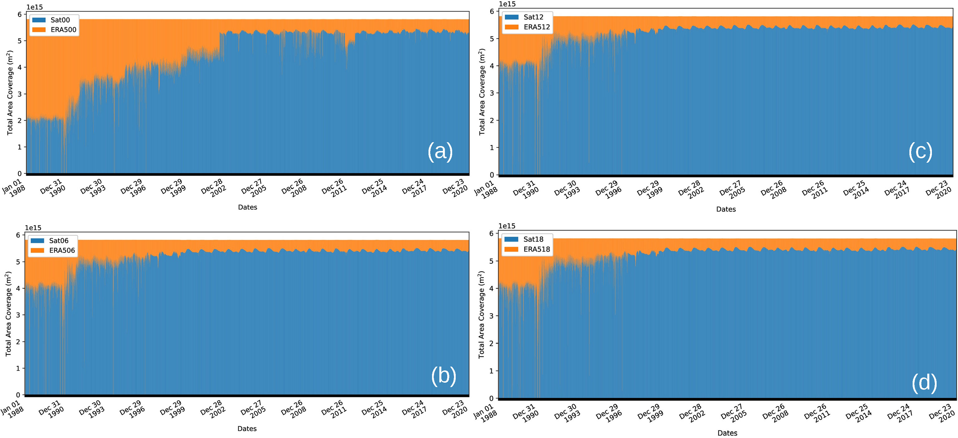
Figure 4 Time series plots of total area coverage for satellite data (in blue) and reanalysis data (in orange) for the period of NBS v2.0. at four different synoptic times (A) 0000 UTC, (B) 0600 UTC, (D) 1200 UTC, and (C) 1800 UTC.

5 Comparison with Copernicus marine environment monitoring service winds

The European CMEMS Wind Thematic Assembly Center (TAC) provides and maintains both Level 3 (L3) and Level 4 (L4) surface winds derived from satellite-based scatterometers and radiometers. The data are provided in both NRT and reprocessed mode (REP) (De Kloe et al., 2017). The L4 data include wind components (meridional and zonal) and wind stress (both components as well) along with other data. These fields are currently available globally in 6-hourly synoptic time (0000, 0600, 1200, and 1800 UTC) with a spatial resolution of 0.25° in longitude and latitude. The reprocessed version of this CMEMS wind data goes back to 1992. In the following, we compare our NBS v2.0 with the CMEMS winds as a product inter-comparison and evaluation exercise.

A matchup dataset is generated on the same spatial and temporal grids for this comparison. Figure 5 shows the mean difference field (CMEMS—NBS v2.0) and root mean square difference (RMSD) between them using a long-term overlap time period from 1992 to 2019.

The mean values of spatial comparison show that on a global scale, the wind values from the NBS wind product are very much similar to the CMEMS data, and the difference field is in and around zero value throughout. The global mean difference values are ~0.03 m/s with some statistically insignificant values between +5 and −5 m/s. The RMSD of the difference field (Figures 5E–H) for all the synoptic time data shows that throughout the equatorial, tropical, and subtropical regions, it ranges from 0 to 2 m/s. In the higher latitudes, the RMSD varies between 3 and 5 m/s. Figure 6 shows the global mean difference (CMEMS—NBS v2.0) time series for the period of 1992 to 2019, with the top panel showing the u-component and the bottom panel the v-component. The different colors (red, blue, green, and orange) denote four different synoptic times (0000, 0600, 1200, and 1800 UTC). It is clear from the time-series data that the global mean values of the two products are very much in agreement, as the different lines fluctuate near the zero-mean line. The long-term mean in the difference field are ~0.04 m/s (0000 UTC), ~0.047 m/s (0600 UTC), ~0.038 m/s (1200 UTC), and ~0.045 m/s (1800 UTC) for the u-component of wind, and these values are respectively −0.027, −0.0275, −0.04, and −0.0277 m/s for the v-component. The corresponding distribution curve in the difference field also shows a quasi-normal distribution with negligible outliers not affecting the overall statistics. On detailed observation of the days where the highest differences are reported, it was found that CMEMS data were erroneous for those few days (e.g., 2000/05/20, 2004/02/27–2004/02/29, and 2009/12/03).

FIGURE 5

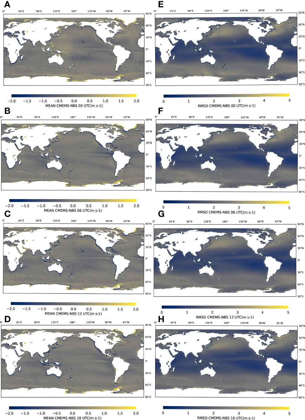
Figure 5 Map of Copernicus Marine Environment Monitoring Service (CMEMS)—NBS v2.0 winds. (A–D) The mean of this difference field. (E–H) The root mean square difference (RMSD) for a time period of 28 years (1992–2019) for four different synoptic times (0000, 0600, 1200, and 1800 UTC).

FIGURE 6

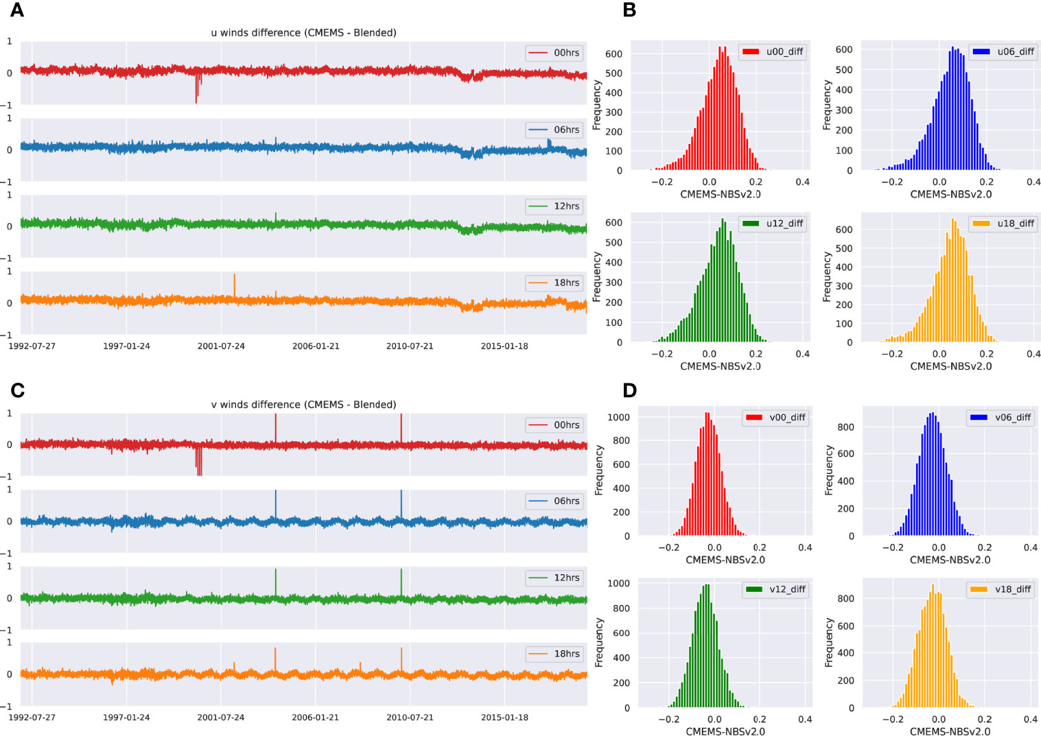
Figure 6 Time series of global annual mean of difference between Copernicus Marine Environment Monitoring Service (CMEMS) and National Oceanic and Atmospheric Administration (NOAA) National Centers for Environmental Information (NCEI) blended wind. A time series of daily global mean in the difference field (CMEMS—NOAA/NCEI blended sea winds) also shows that both the products agree more or less with each other for the entire period of 1992 to 2018, (A) is for the u-component, and (C) is for v-component of wind. The different colors denote different synoptic times. A distribution curve (histogram) for all 6-hourly times is also provided for (B) the u-component and (D) the v-component of wind.

6 Identification, tracking, and characteristics of high winds in NBS v2.0 during hurricanes and tropical cyclones

The new version of NBS is developed using a random-error based weighting factor to resolve very high winds around hurricanes, which are usually missing or underestimated in existing gap-free products. Usually, these fast-moving storms have heavy rainfalls associated with them, and both the active scatterometers and passive radiometers do not resolve such winds due to signal degradation. Recent advancements in satellite wind retrievals revealed that a new L-band instrument onboard the SMAP satellite can provide accurate hurricane winds of up to 65 m/s (145 MPH) without being affected by rain (Meissner et al., 2017). Additionally, the all-weather channel in AMSR-2 is a blend of wind at 6.9 GHz in no rain conditions and a statistical algorithm developed for retrieving accurate winds of up to 70–80 m/s during heavy rains. Both SMAP and AMSR-2 data not only provide these high wind observations but also complement each other and are highly accurate. These high-wind satellite data are infused into our NBS v2.0 with a special technique described in Section 3, and we present some examples of the storm events in this product.

6.1 Tropical Cyclone Fantala

TC Fantala (Figure 7) was one of the strongest cyclones over the western Indian Ocean. It started on 11 April 2016, and reached an intensity of Category 5 (on the Saffir–Simpson wind scale) by 18 April 2016. It started as a weak disturbance at approximately 12.7°S and 62.7°E on 11 April, from where it moved westward rapidly, intensifying and reaching a status of Category 3 (with an average wind speed of 110 knots or 56.5 m/s) by 15 April (Duvat et al., 2017). From 15 to 18 April, the storm hovered between Category 4 and 5 while drifting northeast of Madagascar and hitting Farquhar Atoll in the Seychelles on 17 April. The wind speed by then had reached an estimated 150 knots (77 m/s), as reported by the Joint Typhoon Warning Center (JTWC). By 20 April, Fantala weakened to Category 3, and it continued to weaken thereafter. The storm made a U-turn on 19 April moving more southeastward to a position northeast of Madagascar. TC Fantala weakened further (to Category 2) as it tracked backward to the southeast until 22 April, before making a second U-turn and being downgraded to a weak depression at the end of 22 April.

FIGURE 7

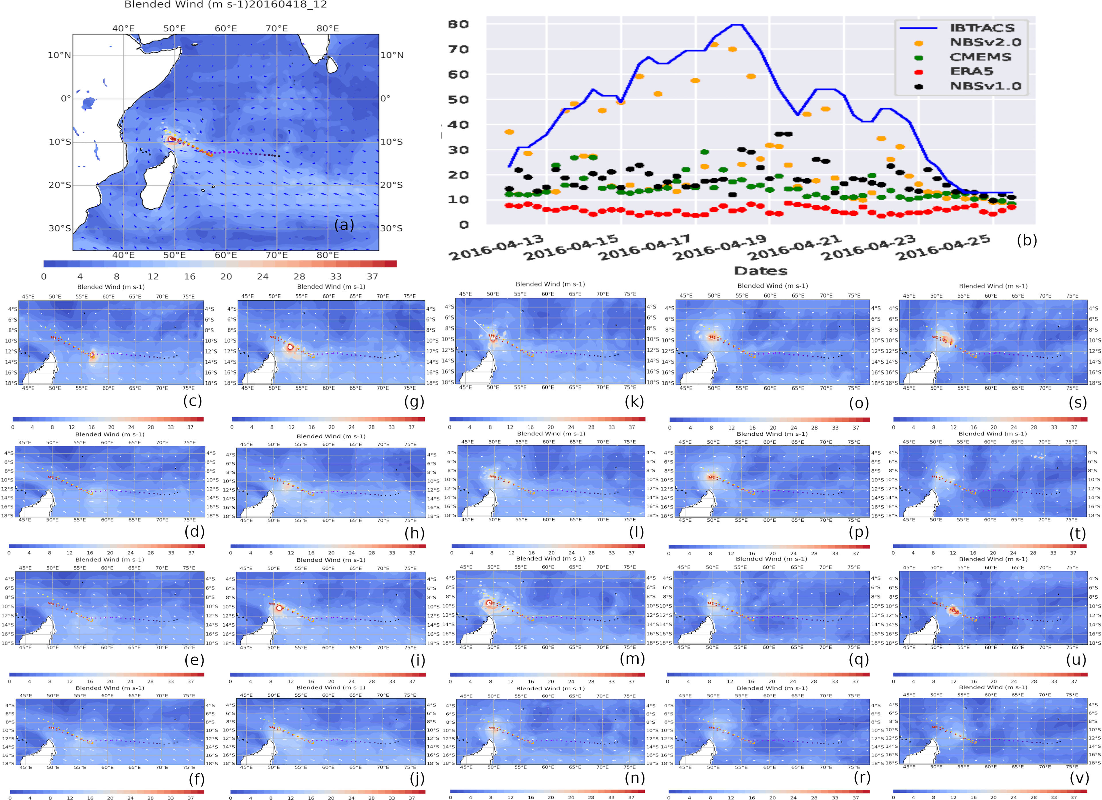
Figure 7 (A) Tropical cyclone Fantala’s maximum wind speed with best track from the IBTrACS data set. (B) Time series of maximum wind along the track of the Tropical Cyclone Fantala. (C–V) Five days of wind data in and around the peak of the storm (on April 18, 2016), for different days (along the rows) and 4 snapshots for each day (along the columns).

Figure 7A shows the TC Fantala’s best track from the IBTrACS dataset (Knapp et al., 2010). IBTrACS provides a collation of currently available best-track data from agencies worldwide, including the World Meteorological Organization (WMO) Regional Specialized Meteorological Centers (RSMCs) and the Tropical Cyclone Warning Centres (TCWCs), as well as other national agencies like the JTWC and NOAA National Hurricane Center (NHC). Figure 7B shows the time series of maximum sustained surface wind speed (MSW) along the track of the storm with blue representing IBTrACS points, and maximum winds in NBS v2.0, CMEMS, ERA-5, and NBS v1.0 represented by orange, green, red, and black, respectively. Figures 7C–V show 5 days of NBS v2.0 wind data in and around the peak of the storm (on 18 April, 2016), with different days (16 April to 20 April, along the rows) and winds for each day at 0000, 0600, 1200, and 1800 UTC.

The maps show clearly that NBS v2.0 is able to capture both the direction of the storm and the high winds associated with the storm. The time-series plot also confirms that NBS v2.0 is able to delineate the very high values of winds in and around the storm eye along the track of TC Fantala, whereas both the CMEMS blended product and ERA-5 reanalysis miss the high values of the winds. NBS v2.0 sometimes misses the high value of the storm as well; it is mainly due to the fact that resolving the high winds depends on the availability and quality of observational data, such as from the SMAP and AMSR2. Therefore, if SMAP or AMSR2 fails to capture the storm or if their data have larger errors, NBS v2.0 cannot resolve the storm winds either.

6.2 Hurricane Irma

Hurricane Irma (Figure 8) was a massive and long-lived hurricane that started from Cape Verde and reached a scale of Category 5 on the Saffir–Simpson scale. The hurricane made 7 catastrophic landfalls from the Caribbean all the way to Florida (Cangialosi et al., 2018). Irma was one of the strongest, costliest, and most devastating storms on record over the Atlantic Basin, which originated over the west coast of Africa in late August 2017. It traveled a long path from the west–southwest of Sao Vicente in the Cabo Verde Islands to the southwest of Florida where it made landfall as a Category 4 hurricane. Figure 8A shows the best track positions for Hurricane Irma. Figure 8B shows the time series of the maximum wind, MSW, along the track of the storm, with blue representing IBTrACS points, and maximum winds from NBS v2.0, CMEMS, ERA-5, and NBS v1.0 represented by orange, green, red, and black, respectively. Figures 8C–V show a snapshot of the NBS v2.0 product for 5 days of the hurricane in and around when it peaked before its final landfall over northern Florida. Irma reached Category 4 as its winds peaked at 155 knots (~79 m/s). None of the globally gridded products but NBS v2.0 are able to capture the high winds along the storm track.

FIGURE 8

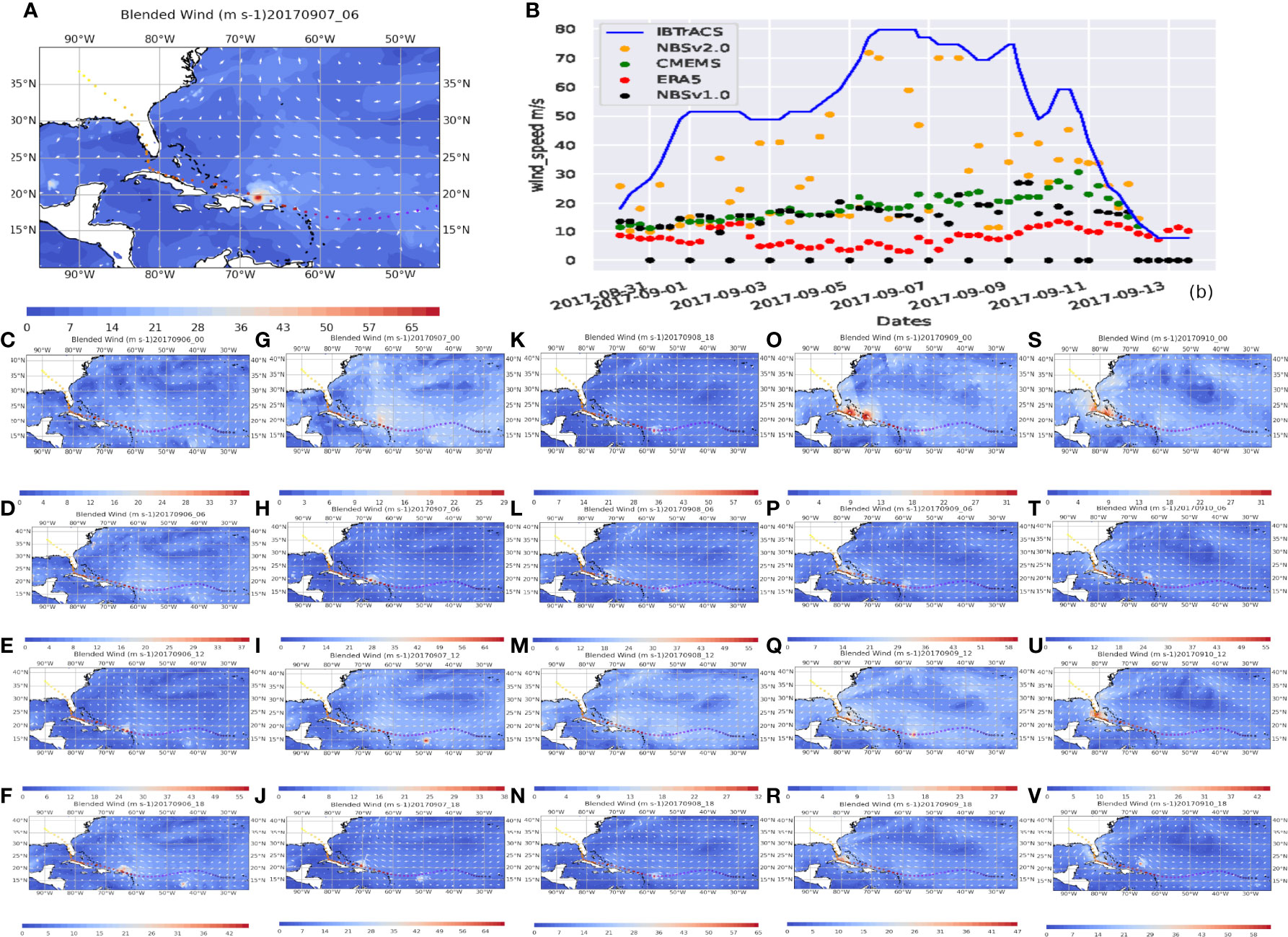
Figure 8 (A) Peak wind speed day of Irma with best track available from IBTrACS data. (B) Time series of maximum wind along the track of Hurricane Irma. (C–V) Five days of wind data in and around the peak of the storm (on 7 September 2017), with different days (along the rows) and 4-hourly winds for each day (along the columns).

6.3 Tropical Cyclone Amphan

Super Cyclonic Storm Amphan (Figure 9) was a powerful and catastrophic TC that formed over the north of the Bay of Bengal (BoB) in May 2020. On 13 May 2020, Amphan originated from a low-pressure region a few hundred miles off the east of Colombo, Sri Lanka. By 17 May, this extremely severe cyclonic storm had sustained winds of approximately 94 knots (48 m/s) equivalent to a Category 2 storm. Amphan quickly intensified into a Category 5 storm on 18 May, with sustained winds of 145 knots (~75 m/s). Such high winds were sufficient to classify Amphan as a super cyclone over the BoB basin. Given the location of the storm, it caused a tremendous amount of loss of life and destruction in that region. By the afternoon of 20 May at landfall, the winds were of the order of 75 knots (~38 m/s), but the storm remained powerful enough to destroy the coastal area (Ahmed et al., 2021).

FIGURE 9

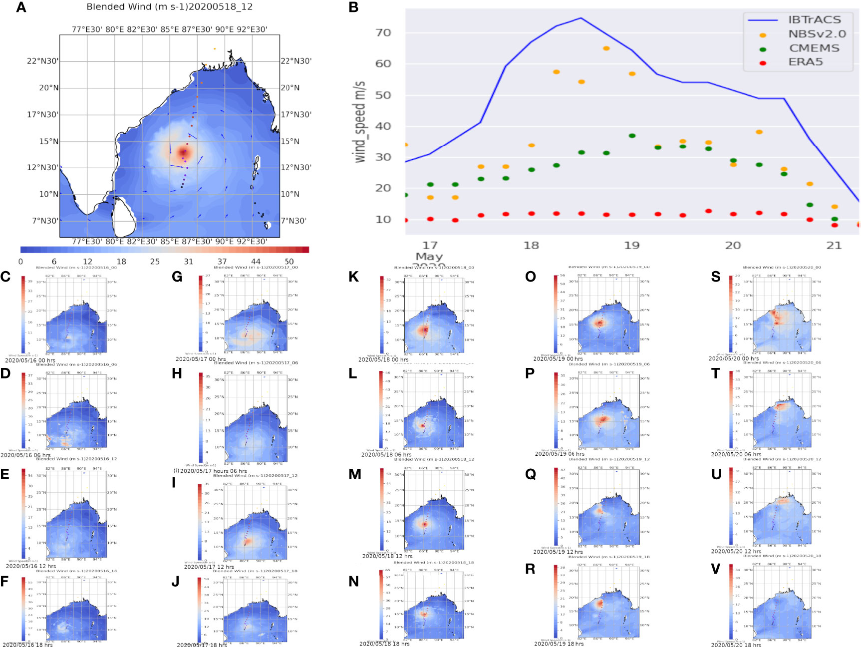
Figure 9 (A) Wind speed with track available from IBTrACS data. (B) Time series of maximum wind along the track of the Tropical Cyclone (TC) Amphan. (C–V) Five days of wind data in and around the peak of the storm (on 18 May 2020), with different days (along the rows) and 4-hourly winds for each day (along the columns).

Figure 9A shows the best track positions for TC Amphan available from IBTrACS data. Figure 9B shows the time series of MSW, along the track of the storm with blue representing IBTrACS points, and maximum winds for NBS v2.0, CMEMS, ERA-5, and NBS v1.0 are represented by orange, green, red, and black, respectively. Figures 9C–V show the new NBS product for 5 days of the super cyclone in and around when it peaked before its final landfall over the Indo-Bangladesh coast at approximately 1200 UTC on 20 May. Throughout the best track of the storm, the MSW values from IBTrACS data clearly match better with NBS v2.0 winds as compared to the CMEMS and ERA-5. For IBTrACS, the wind ranges from 19 to as high as 75 m/s, whereas for the NBS v2.0, this value ranges from 10 to 65 m/s. CMEMS winds range from 10 to 38 m/s, and ERA-5 was always underestimating at ~10 m/s. Therefore, it can be inferred that the NBS v2.0 product is performing better than the other existing blended and reanalysis data. The maps also capture the formation of the storm in such a short period of time, with sudden increases in wind speeds from about 40 to about 65 m/s when it peaked at approximately 13°N and 87°E on 18 May. The eye of the storm follows the best track position from IBTrACS from its genesis to the final landfall at the Indo-Bangladesh border on 20 May.

7 Summary and conclusion

The production of globally gridded gap-free 10-m neutral wind data that can resolve very high winds in and around TCs and hurricanes is one of the needed features for improving ocean, weather, and climate forecasts and research. Most of the existing globally gridded products and/or reanalysis products are not able to delineate the high wind values along the path of a passing storm. The NOAA NCEI Blended Sea winds (NBS) v2.0 is a new improved version over the existing v1.0 and in particular, is now capable of resolving high storm winds. NBS v2.0 is developed to include the new satellite retrieved winds from the L-band instrument on SMAP and the all-weather channel of AMSR2, along with the existing microwave imagers and scatterometers. Along with a spatial–temporal weighted interpolation, the storm-wind resolving SMAP and AMSR2 data are added to the blended sea winds product using a multi-sensor data fusion technique based on random errors.

The NBS v2.0 is generated from a combination of neutral winds derived from multiple satellites that are calculated from surface stress and roughness length by assuming that ideally the air is neutrally stratified. For moderate and strong winds over the open ocean, when shear production dominates over buoyancy production of turbulence, the effect of atmospheric stratification is minimal. Therefore, in reality, although the neutral conditions are rare, on an average for a marine boundary layer weekly unstable condition, the global mean 10-m neutral winds appear to be ~0.19 m/s stronger than the non-neutral wind (Brown et al., 2006; also see discussions at https://www.coaps.fsu.edu/~bourassa/BVW_html/eqv_neut_winds.php#:~:text=In%20the%20most%20common%20definition,%5BGeernaert%20and%20Katsaros%201986%5D).

The NBS v2.0 contains a long-term sea surface wind product from 1987 to the present that can easily delineate high storm winds starting from 2012 onward when the SMAP’s and/or AMSR2’s all-weather channel data become available. This product is examined for multiple cases of TCs and hurricanes, and three of them are presented here. Comparisons with the IBTrACS data show that NBS v2.0 performs better than the other existing globally gridded gap-free blended and reanalysis products. NBS v2.0 is also operationally updated in two modes: one is the NRT (v2.0_nrt) data with a latency of 1 day, using NRT preliminary versions of satellite data and NOAA/NCEP/GFS model data. Then on a monthly basis, the NRT version is replaced by reprocessing using the updated science quality satellite data and ERA5 reanalysis data. The NBS v2.0 (including the NRT v2.0_nrt) data will be publicly available through NOAA’s Coast Watch and Ocean Watch and archived at NCEI. In the future, we plan to include wind data retrieved from other satellites like SMOS, SAR data from Sentinal-1A/1B, and high-resolution CYGNSS data to improve the product on both global and regional scales.

Data Availability Statement

The raw data supporting the conclusions of this article will be made available by the authors, without undue reservation.

Author Contributions

Both authors were involved in the development of a new version of this product. Most of the analysis was conducted by KS. The manuscript was written by KS, with input from H-MZ. All authors read and approved the final manuscript.

Conflict of Interest

The authors declare that the research was conducted in the absence of any commercial or financial relationships that could be construed as a potential conflict of interest.

Publisher’s Note

All claims expressed in this article are solely those of the authors and do not necessarily represent those of their affiliated organizations, or those of the publisher, the editors and the reviewers. Any product that may be evaluated in this article, or claim that may be made by its manufacturer, is not guaranteed or endorsed by the publisher.

Acknowledgments

The authors would like to acknowledge numerous feedbacks and discussions from our product users, which motivated us to develop this blended wind product that can delineate very high winds associated with hurricanes/tropical cyclones. We would like to thank Ken Knapp and his team for developing and maintaining this amazing storm tracks data called IBTrACS, NCEI internal reviewers for their comments that substantially improved the manuscript, and Jennifer Fulford and our internal editorial staff for editorial improvement. Dr. Korak Saha is supported by a NOAA/NCEI grant to the University of Maryland through CISESS.

References

Ahmed R., Mohapatra M., Dwivedi S., Giri R. K. (2021). Characteristic Features of Super Cyclone ‘Amphan’- Observed Through Satellite Images.Trop. Cyclone Res. Rev. 10 (1), 16–31. doi: 10.1016/j.tcrr.2021.03.003

CrossRef Full Text | Google Scholar

Atlas R., Hoffman R. N., Ardizzone J., Leidner S. M., Jusem J. C., Smith D. K., Gombos D. (2011). A Cross-Calibrated, Multiplatform Ocean Surface Wind Velocity Product for Meteorological and Oceanographic Applications. Bull. Am. Meteorolog. Soc. 92 (2), 157–174. doi: 10.1175/2010bams2946.1

CrossRef Full Text | Google Scholar

Bonjean F., Lagerloef G. S. E. (2002). Diagnostic Model and Analysis of the Surface Currents in the Tropical Pacific Ocean. J. Phys. Oceanogr. 32 (10), 2938–2954. doi: 10.1175/1520-0485(2002)032<2938:DMAAOT>2.0.CO;2

CrossRef Full Text | Google Scholar

Brown A. R., Beljaars A. C. M., Hersbach H. (2006). Errors in Parametrizations of Convective Boundary-Layer Turbulent Momentum Mixing. Q. J. R. Meteorolog. Society. R. Meteorolog. Soc. (Great Britain) 132 (619), 1859–1876. doi: 10.1256/qj.05.182

CrossRef Full Text | Google Scholar

Cangialosi J. P., Latto A. S., Berg R. (2018). National Hurricane Center Report: Hurricane IRMA 30 August–12 September 2017 ( National Oceanic and Atmospheric Administration and National Hurricane Center). Available at: https://www.nhc.noaa.gov/data/tcr/AL112017_Irma.pdf.

Google Scholar

De Kloe J., Stoffelen A., Verhoef A. (2017). “The CMEMS L3 Scatterometer Wind Product,” in EGU General Assembly Conference Abstracts. Geophysical Res. Abstracts 19, EGU2017–18763, EGU General Assembly 2017.

Google Scholar

Desbiolles F., Bentamy A., Blanke B., Roy C., Mestas-Nuñez A. M., Grodsky S. A., (2017). Two Decades [1992–2012] of Surface Wind Analyses Based on Satellite Scatterometer Observations. J. Mar. systems: J. Eur. Assoc. Mar. Sci. Techniques 168, 38–56. doi: 10.1016/j.jmarsys.2017.01.003

CrossRef Full Text | Google Scholar

Domingues R., Kuwano-Yoshida A., Chardon-Maldonado P., Todd R. E., Halliwell G., Kim H.-S., (2019). Ocean Observations in Support of Studies and Forecasts of Tropical and Extratropical Cyclones. Front. Mar. Sci. 6. doi: 10.3389/fmars.2019.00446

CrossRef Full Text | Google Scholar

Duvat V. K. E., Volto N., Salmon C. (2017). Impacts of Category 5 Tropical Cyclone Fantala (April 2016) on Farquhar Atoll, Seychelles Islands, Indian Ocean. Geomorphology 298, 41–62. doi: 10.1016/j.geomorph.2017.09.022

CrossRef Full Text | Google Scholar

Entekhabi D., Das N., Yueh S., De Lannoy G., O'Neill P. E., Dunbar R. S., Kellogg K. H., (2014). SMAP Handbook ( Jet Propulsion Laboratory Publ. JPL), 400–1567. Available at: https://smap.jpl.nasa.gov/system/internal_resources/details/original/178_SMAP_Handbook_FINAL_1_JULY_2014_Web.pdf.

Google Scholar

Gao S., Zhong Y., Li W. (2011). Random Weighting Method for Multisensor Data Fusion. IEEE Sensors J. 11 (9), 1955–1961. doi: 10.1109/jsen.2011.2107896

CrossRef Full Text | Google Scholar

Knapp K. R., Kruk M. C., Levinson D. H., Diamond H. J., Neumann C. J. (2010). The International Best Track Archive for Climate Stewardship (IBTrACS): Unifying Tropical Cyclone Data. Bull. Am. Meteorolog. Soc. 91 (3), 363–376. doi: 10.1175/2009bams2755.1

CrossRef Full Text | Google Scholar

McColl K. A., Ogelzang J., Konings A. G., Entekhabi D., Piles M., Stoffelen A. (2014). Extended Triple Collocation: Estimating errors and Correlation Coefficients with Respect to an Unknown Target.Geophys. Res. Lett. 41(17). doi: 10.1002/2014GL061322

CrossRef Full Text | Google Scholar

Meissner T., Ricciardulli L., Manaster A. (2021). Tropical Cyclone Wind Speeds From WindSat, AMSR and SMAP: Algorithm Development and Testing. Remote Sens. 13 (9), 1641. doi: 10.3390/rs13091641

CrossRef Full Text | Google Scholar

Meissner T., Ricciardulli L., Wentz F. (2017). Capability of the SMAP Mission to Measure Ocean Surface Winds in Storms. Bull. Am. Meteorolog. Soc. 98, 1660–1677. doi: 10.1175/BAMS-D-16-0052.1

CrossRef Full Text | Google Scholar

Meissner T., Ricciardulli L., Wentz F. (2018). Remote Sensing Systems SMAP Daily Sea Surface Winds Speeds on 0.25 Deg Grid, Version 01.0 [NRT or FINAL] (Santa Rosa, CA: Remote Sensing Systems). Available at: www.remss.com/missions/smap.

Google Scholar

Reul N., Tenerelli J., Chapron B., Vandemark D., Quilfen Y., Kerr Y. (2012). SMOS Satellite L-Band Radiometer: A New Capability for Ocean Surface Remote Sensing in Hurricanes. J. Geophys. Res. 117, C02006 (1–24). doi: 10.1029/2011jc007474

CrossRef Full Text | Google Scholar

Ricciardulli L., Wentz F. J. (2016). Remote Sensing Systems ASCAT C-2015 Daily Ocean Vector Winds on 0.25 Deg Grid, Version 02.1 (Santa Rosa, CA: Remote Sensing Systems). Available at: http://www.remss.com/missions/ascat.

Google Scholar

Ricciardulli L., Wentz F. J., Smith D. K. (2011). Remote Sensing Systems QuikSCAT Ku-20112011 [Indicate Whether You Used Daily, 3-Day, Weekly, or Monthly] Orbital Swath Ocean Vector Winds L2B, Version 4, [Indicate Subset If Used] (Santa Rosa, CA: Remote Sensing Systems). Available at: https://www.remss.com/missions/qscat.

Google Scholar

Saha K., Dash P., Zhao X., Zhang H.-m. (2020). Error Estimation of Pathfinder Version 5.3 Level-3C SST Using Extended Triple Collocation Analysis. Remote Sens. 12 (4), 590. doi: 10.3390/rs12040590

CrossRef Full Text | Google Scholar

Salvadori G., De Michele C., Kottegoda N. T., Rosso R. (2007). Extremes in Nature: An Approach Using Copulas. Water Science and Technology Library Vol. Vol. 56 (Dordrecht: Springer Netherlands). doi: 10.1007/1-4020-4415-1

CrossRef Full Text | Google Scholar

Villas Bôas A. B., Ardhuin F., Ayet A., Bourassa M. A., Brandt P., Chapron B., (2019). Integrated Observations of Global Surface Winds, Currents, and Waves: Requirements and Challenges for the Next Decade. Front. Mar. Sci. 6. doi: 10.3389/fmars.2019.00425

CrossRef Full Text | Google Scholar

Wentz F. J., Ricciardulli L., Gentemann C., Meissner T., Hilburn K.A., Scott J. (2013). Remote Sensing Systems Coriolis WindSat [Indicate Whether You Used Daily, 3-Day, Weekly, or Monthly] Environmental Suite on 0.25 Deg Grid, Version 7.0.1, [Indicate Subset If Used] (Santa Rosa, CA). Available at: https://www.remss.com/missions/windsat.

Google Scholar

Wentz F. J., Meissner T., Gentemann C., Brewer M. (2014a). Remote Sensing Systems AQUA AMSR-E [Indicate Whether You Used Daily, 3-Day, Weekly, or Monthly] Environmental Suite on 0.25 Deg Grid, Version 7 [Indicate Subset If Used] (Santa Rosa, CA: Remote Sensing Systems). Available at: https://www.remss.com/missions/amsre.

Google Scholar

Wentz F. J., Meissner T., Gentemann C., Hilburn K. A., Scott J. (2014b). Remote Sensing Systems GCOM-W1 AMSR2 [Indicate Whether You Used Daily, 3-Day, Weekly, or Monthly] Environmental Suite on 0.25 Deg Grid Version 8.2, [Indicate Subset If Used] (Santa Rosa, CA: Remote Sensing Systems). Available at: https://www.remss.com/missions/amsr/.

Google Scholar

Wentz, Meissner T., Scott J., Hilburn K. A.(2015b). Remote Sensing Systems GPM GMI [Indicate Whether You Used Daily, 3-Day, Weekly, or Monthly] Environmental Suite on 0.25 Deg Grid, Version 8.2 [Indicate Subset If Used] (Santa Rosa, CA: Remote Sensing Systems). Available at: http://www.remss.com/missions/gmi.

Google Scholar

Wentz F. J., Gentemann C., Hilburn K. A. (2015a). Remote Sensing Systems TRMM TMI [Indicate Whether You Used Daily, 3-Day, Weekly, or Monthly] Environmental Suite on 0.25 Deg Grid, Version 7.1, [Indicate Subset If Used] (Santa Rosa, CA: Remote Sensing Systems). Available at: http://www.remss.com/missions/tmi.

Google Scholar

Wentz F. J., Hilburn K. A., Smith D. K. (2012). Remote Sensing Systems DMSP [SSM/I or SSMIS] [Daily, 3-Day, Weekly, Monthly] Environmental Suite on 0.25 Deg Grid, Version 7, [Indicate Subset If Used] (Santa Rosa, CA: Remote Sensing Systems). Available at: https://www.remss.com/missions/ssmi.

Google Scholar

Zeng L., Levy G. (1995). Space and Time Aliasing Structure in Monthly Mean Polar-Orbiting Satellite Data. J. geophys. Res. 100 (D3), 5133. doi: 10.1029/94jd03252

CrossRef Full Text | Google Scholar

Zhang H.-M., Reynolds R. W., Bates J. J. (2006). “Blended and Gridded High Resolution Global Sea Surface Wind Speed and Climatology From Multiple Satellites: 1987-Present,” in 14th Conference on Satellite Meteorology and Oceanography.

Google Scholar