Diver-generated photomosaics as a tool for monitoring temperate rocky reef ecosystems

1 Introduction

Globally, human activities are increasingly shaping ecosystems, though direct and indirect pathways such as climate change, species invasion, habitat modification, and harvest. Well-designed monitoring programmes can evaluate key ecosystem trends and inform management, conservation and restoration initiatives (Lovett et al., 2007; Lindenmayer and Likens, 2010; Mihoub et al., 2017). Traditionally, ecosystem monitoring has involved manual data collection in the field, which provides high quality data, but typically at low spatial and temporal scales due to the high effort and acquisition costs required. This creates data collection trade-offs (Braunisch and Suchant, 2010; Del Vecchio et al., 2019; D'Urban Jackson et al., 2020). For example, increasing the spatial scale may require reducing the amount of data collected at each site. Thus, alternative methods of data collection have been sought.

Recent developments in cost effective remote sensing techology such as high resolution satellites and unmanned aerial vehicles (UAVs) have revolutionised many forms of ecological monitoring, particularly in terrestrial environments (Aplin, 2005; Klemas, 2015; Yao et al., 2019). Imagery from these technologies, coupled with powerful computing software, allow rapid data collection and analysis over greater spatial scales and improved access to remote and less accessible locations (Klemas, 2015). The speed, access, and image quality can help to alleviate some of the trade-offs between monitoring effort and data quality and quantity that arise from traditional in-field data collection methods, enabling a better understanding of environmental change by allowing larger quantities of detailed data to be collected or over larger spatial scales during the same time frame.

Marine ecosystems are typically difficult to access and expensive to monitor. The impacts of human activities are acutely felt in coastal and nearshore marine regions (Halpern et al., 2008) where the cumulative effects of climate change, overfishing and terrestrial runoff result in large-scale ecosystem degradation and collapse (Halpern et al., 2019). Benthic ecosystems are particularly vulnerable as many species are sessile or have limited mobility and are unable to avoid disturbance (Solan et al., 2004). Nearshore, shallow subtidal benthic ecosystems have traditionally been monitored through in situ observations made by SCUBA divers with tools such as quadrats and transect tapes. These methods are time consuming and consequently spatially limited, and are prone to observer variability (Pizarro et al., 2017; Marre et al., 2020). Alternatively, aerial imagery and remote sensing data from satellite and UAVs can increase the spatial coverage, but often lack the resolution required to detect fine scale benthic patterns (Mizuno et al., 2017) and are restricted by water clarity, tides and meterological conditions, limiting their usefulness to very clear water habitats (Casella et al., 2017) or shallow depths, such as near surface kelp cover (Bennion et al., 2019; Tait et al., 2019; Cavanaugh et al., 2021).

Underwater structure-from-motion (SfM) photogrammetry presents a useful middle ground, allowing rapid, fine scale benthic observations to be made over larger spatial scales than are possible using traditional methods. Imagery for underwater SfM photogrammetry can be collected by divers with handheld cameras (Bayley and Mogg, 2020), by systems towed behind a vessel (Fakiris et al., 2022) and using remotely operated vehicle (ROV) or autonomous underwater vehicle (AUV) technology (Ling et al., 2016; Teague and Scott, 2017). While the extraction of benthic data from underwater photos, photo-quadrats and video (photogrammetry) is not new (Bohnsack, 1979; Logan et al., 1984; Roberts et al., 1994; Preskitt et al., 2004), improvements in computing power and photogrammetric software have allowed SfM to become a powerful, flexible tool for benthic monitoring and research, providing more methodological options for collecting data that fits intended study aims. SfM photogrammetry reconstructs a three-dimensional (3D) scene or feature from a series of overlapping two-dimensional (2D) images (Bayley and Mogg, 2020). Underwater SfM image acquisition of large areas is rapid (110 m² can be covered in approximately 15 min by a diver [Pizarro et al., 2017]), can be collected with low-cost camera equipment (Raoult et al., 2016) and resulting reconstruction resolution can be cm - mm per pixel due to the proximity of image capture (Marre et al., 2019). Reconstructions can also be orthorectified (correctly scaled) by using ground control points, scale references and/or GPS, allowing for standardised, accurate measurements (Burns et al., 2015; Teague and Scott, 2017; Marre et al., 2019; Nocerino et al., 2020). The SfM process produces a range of 2D or 3D outputs including photomosaics, digital elevation models, 3D meshers and point clouds. Photomosaics, 2D data, allow extraction of biological metrics such as species counts and cover percentages which can be used for calulating community composition, density and diversity (Raoult et al., 2016; Mizuno et al., 2017; Marre et al., 2019). 3D data can also provide information on structural complexity, species morphometrics and biomass (Palma et al., 2018; Bayley et al., 2019), which are frequently used for ecosystem monitoring. Machine learning classifiers, such as object based image analysis (OBIA), can further enhance the utility of these data formats by allowing the semi- or fully automatic classification of features (De Oliveira et al., 2021; Ternon et al., 2022).

Despite the surge in popularity of diver-based SfM photogrammetry for gathering benthic data in shallow water tropical ecosystems, similar examples from temperate regions remain limited. Temperate nearshore subtidal ecosystems are typically turbid environments when compared to their tropical counterparts making SfM image capture a greater challenge (Lochhead and Hedley, 2022; Ternon et al., 2022). Wave action is particularly problematic on rocky reefs dominated by kelp or other algae. These non-rigid taxa will continuously move in relation to water motion which has the potential to hinder the SfM reconstruction process, as has been shown in terrestrial systems when surveying vegetation in windy conditions (Dandois et al., 2015; Fraser and Congalton, 2018). Diver-based SFM photogrammetry work on algal dominated rocky reefs has to date been limited in spatial scale and focussed on measuring a single metric such as reef rugosity (Monfort et al., 2021), substrate composition (Ternon et al., 2022) or quantifying crustose coralline algae cover underneath kelp canopies (Smale et al., 2020). The potential for using SfM photogrammetry for collecting data from temperate rocky reef ecosystems, particularly as an alternative to, or supplement to traditional SCUBA-based methods for benthic monitoring, requires further investigation.

Here we assess the use of diver-generated photomosaics, a 2D SfM photogrammetry output, for extracting biotic data used for ecosystem monitoring from subtidal rocky reefs along the north-eastern coastline of New Zealand. This coastline has been subjected to significant commercial and recreational fishing pressure since the early 1900s which has resulted in significant declines in the abundance of predatory snapper (Chrysophrys auratus) and lobster (Jasus edwardsii; Francis and McKenzie, 2015; Webber et al., 2018). Without top-down predatory pressure, overgrazing by the sea urchin Evechinus chloroticus has transformed areas of productive Ecklonia radiata kelp forest to relatively impoverished urchin barren (Shears and Babcock, 2002). Consequently, urchin barrens are now commonly found on rocky reefs between 2 – 9 m deep along much of the north-eastern New Zealand coastline (Shears and Babcock, 2004). Benthic monitoring within these ecosystems has traditionally been carried out by divers using field quadrats, which is resource and time intensive resulting in limited spatial and temporal sampling. To assess the potential of photomosaics as a monitoring tool we compared data collected from photomosaics to that of traditional quadrats surveys at three sites primarily characterised by urchin barrens within north-eastern New Zealand. At each site SCUBA divers surveyed transects across the reef using quadrats. At the same time, overlapping imagery of the surveyed reef areas was collected and photomosaics created. From these mosaics sea urchin densities, benthic community composition and macroalgae canopy cover, primary metrics recorded in traditional field quadrats, were extracted for comparison. Data collection time for these metrics from both methods was also noted. We discuss these findings along with the strengths and weaknesses of using photomosaics as a monitoring tool within temperate rocky reef ecosystems.

2 Methods and materials

2.1 Field sites

The three sites selected for this study were within within Tık̄apa Moana Hauraki Gulf north-eastern New Zealand (Figure 1). All sites were gradually sloping rock reefs that had been significantly impacted by sea urchin overgrazing. The reefs were characterised by a narrow band of mixed algae in the shallows (~ 0-2 m, mostly E. radiata and Carpophyllum spp.), extensive sea urchin barrens and a deeper E. radiata kelp forest. These sites also spanned an environmental gradient of increasing wave exposure and decreasing sedimentation from inner to outer Gulf (Seers and Shears, 2015). As such the lower depth range of the urchin barrens, which is influenced by wave action (Shears and Babcock, 2004), varied from 5–7 m at Leigh, (sheltered bay) to 8-9 m at Hauturu-o-Toi (the most exposed site with the clearest water).

FIGURE 1

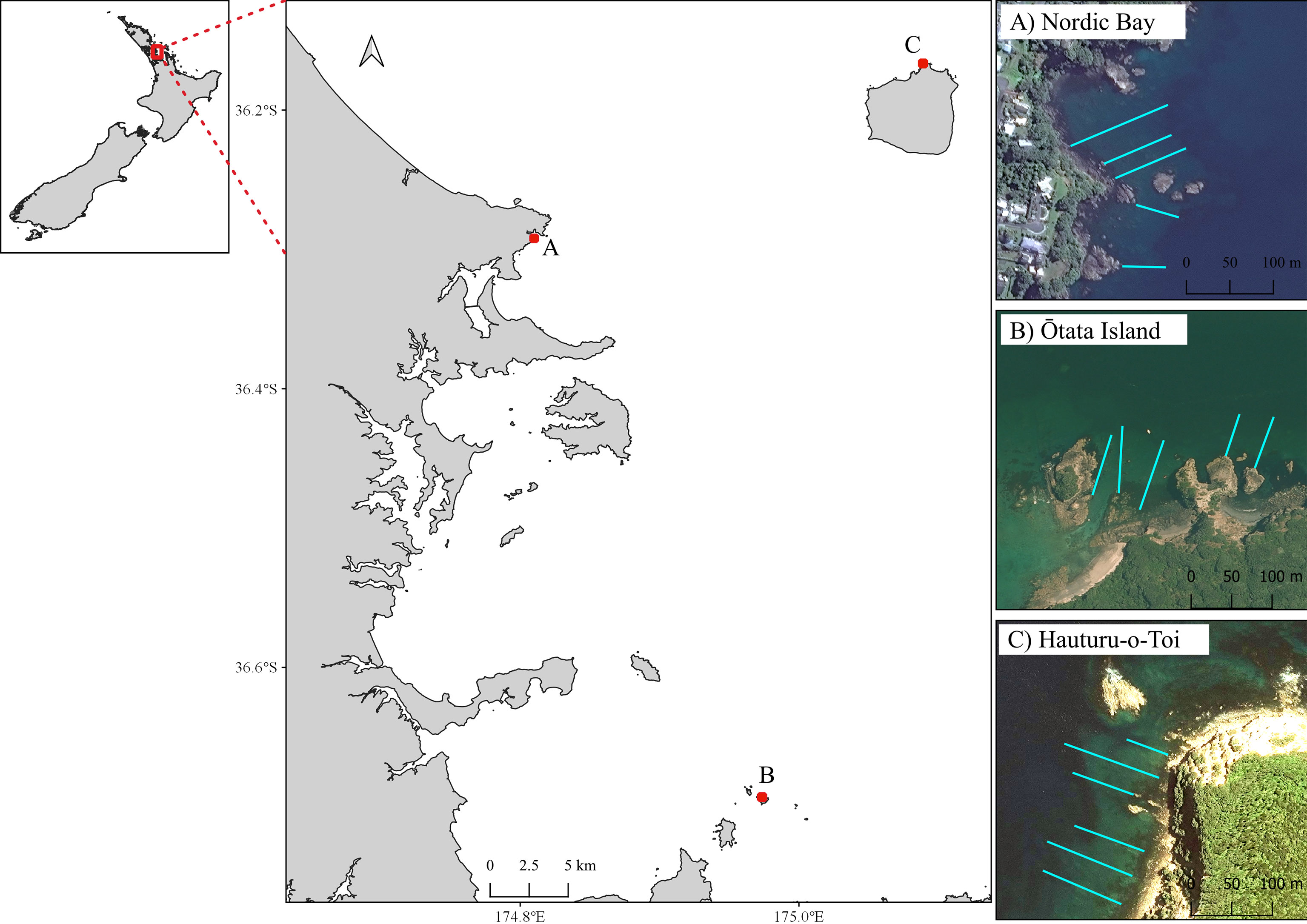
Figure 1 Map of Hauraki Gulf in north-eastern New Zealand, with three benthic monitoring sites: (A) Leigh, (B) Ōtata (inner Gulf); and (C) Hauturu-o-Toi (offshore island). Turquoise lines show approximate transect location.

At each site, line transects were laid out perpendicular to the shoreline on a fixed bearing (Figure 1). These ran from the upper limits of the subtidal zone (mean low water [MLW]), through the extent of the urchin barren (the primary area of monitoring focus) to the shallow edge of the kelp forest, sand, or approximately 100 m (~10 m depth), whichever came first. Markers were present every five meters along each transect line. Photogrammetric scale bars (25 cm x 12.5 cm) were placed along the transect length to aid the 3D model reconstruction process. Each scale bar had six visible markers, with exact distance between marker used for accurate scale during the photomosaic processing. Start and end points for each transect were marked by GPS and with heavy weights with subsurface floats. Five transects were surveyed at Leigh and Ōtata, and six surveyed at Hauturu-o-Toi (Table 1).

TABLE 1

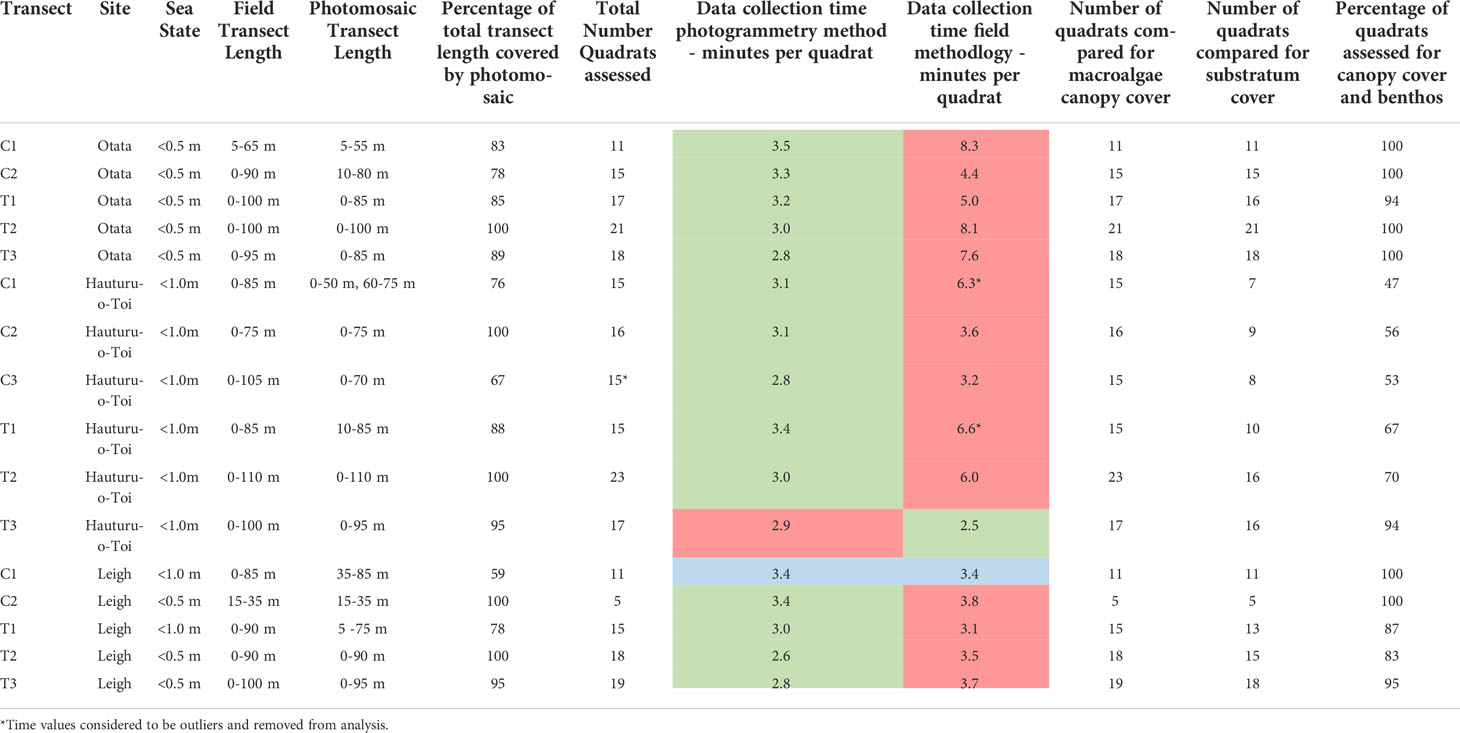
Table 1 Key comparison metrics for each transect between SfM photomosaics and field quadrats. Data collection times are highlighted in red if they were slower, green if faster and blue if the same.

Data on macroalgae canopy cover, sea urchin density and benthic community composition were collected at Ōtata in November 2020 and at Hauturu-o-Toi in March 2021. Macroalgal cover and benthic community composition data was collected at Leigh in April 2021 however, sea urchin density data was only collected from two transects (C1 and C2; Figure 1, Table 1). This was because sea urchins had been removed from T1 – T3 prior to the benthic survey for a simultaneous project.

Here benthic community composition refers to the sessile biotic taxa and abiotic substrates occupying space on the rocky reef. Benthic community composition categories were selected a priori, with the same categories used in the traditional and photogrammetric surveys for consistency (Table S1).

2.2 Traditional field quadrat surveys

A team of two divers collected benthic information along each transect line at 5 m marked intervals, adapted from methods in Shears and Babcock (2004). At each interval, a 1 m² quadrat was placed on the reef to assess in situ macroalgae canopy cover, sea urchin densities, and the benthic community composition. Canopy cover of large brown macroalgae (by species) and benthic community composition categories were visually estimated and expressed as percent covers. To provide an overview of each quadrat a photo was captured using a GoPro Hero 7. The total time taken for each dive team to collect this information from each transect was recorded. Additional information collected by divers but not compared with photomosaic survey include general habitat category, substrate type, depth, abundance and size categories of laminarian (to 25 cm) or fucoid kelps (< or > 25 cm), abundance of large mobile invertebrates, and size categories (to 20 mm) and behaviour of sea urchins. The time taken to collect this additional information was not included into the data collection time analysis, however it was estimated to add an additional 10-20% to the total time taken to collect data from within field quadrats at each site.

2.3 Photomosaic survey

2.3.1 Image collection

Concurrent with the field quadrat surveys, a diver carried out a photographic survey of each transect using methods adapted from previous papers such as Suka et al. (2019) which have collected imagery suitable to produce photomosaics (Figure 2A). Using a wide-angle underwater camera (Nikon Z6 with 14 mm rectilinear lens) the diver slowly swam (~14 m/min) a single pass over each transect line at a distance of 1 – 1.5 m above the benthos. Imagery geospatial information (longitude, latitude and depth) was collected along each transect using an ultra-short baseline underwater geolocation system (UWIS^®, x,y absolute accuracy ± 2.5 m). Total time taken to collect the images per dive was recorded after each transect. The camera was orientated directly downward and recorded an image every second, resulting in ~80% overlap between sequential images. Camera settings were aperture priority (f8) with ISO 800 – 3200. These settings allowed for consistent lighting across the length of the each transect, while enabling a high enough shutter speed to counter the effects of motion blur.

FIGURE 2

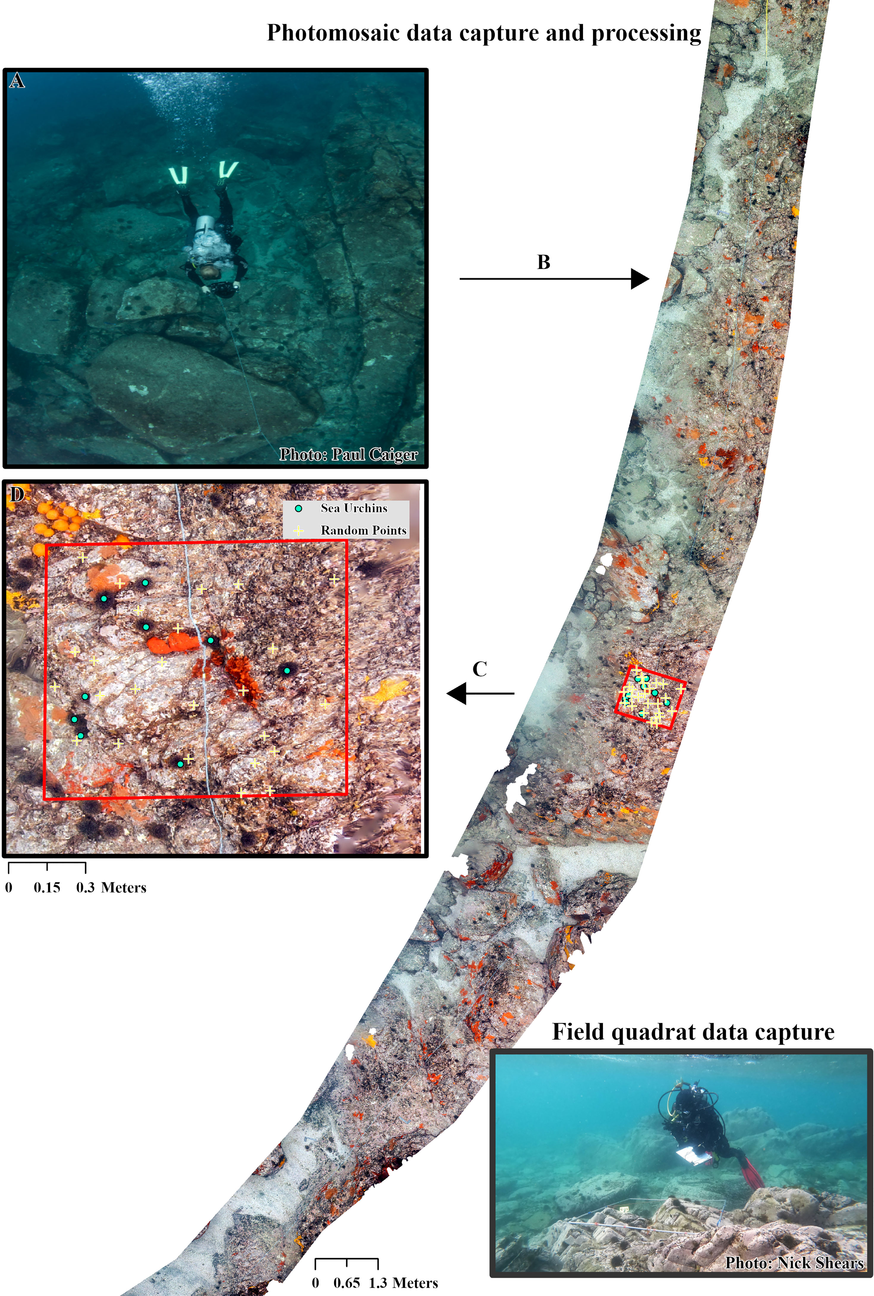
Figure 2 Photomosaic data capture and processing. (A) Capture of raw imagery in the field, (B) image processing and creation of photomosaic, (C) transfer of photomosaic raster into GIS software and (D) placement of virtual quadrats, annotation of random benthic community points and marking of sea urchins. Transect line is visible crossing through the quadrat position. Insert Diver collecting data from field quadrat.

2.3.2 Photomosaic assembly

Using the neutral grey tone of the scale bars, image sets for each transect were batch processed to correct for white balance in Adobe Lightroom before being imported into Agisoft Metashape (Professional V1.7) to create the photomosaics (Figure 2B). This was deemed a more appropriate method for ensuring correct colour within the image set than setting the white balance manually in the field as it avoided the need to stop and adjust white balance as depth changed over the length of the transect. Photomosaics were produced using a process similar to that outlined in Bayley and Mogg (2020). Imagery was first aligned (Accuracy = High, Generic preselection, Tie point limit = 70,000, Key point limit = 7,000), creating a sparse point cloud. Model accuracy was refined using the gradual selection tool to remove points with high reconstruction uncertainty, high projection error and poor projection accuracy (Threshold values of 20, 0.5 and 4 respectively). Each sparse cloud was then scaled using image geospatial reference information, checked using the photogrammetric scale bars placed along the transect line and refined using between marker distances. The sparse cloud was re-optimised, and a dense cloud created (Quality = High, Depth filtering = Mild). A digital elevation model (DEM) was produced from the point cloud which then allowed for the photomosaic to be created (Surface = DEM, blending mode = Mosaic, Hole filling and ghosting filter enabled). As with Raoult et al. (2016) photomosaic assembly time was not included in the data collection time analysis because much of this process is automated. Additionally, the total processing time is dependent on camera image resolution, the number of images being processed and computing power available for use (Bayley and Mogg, 2020; Couch et al., 2021).

2.3.3 Data extraction

Photomosaics were imported into ArcGIS Pro (V2.8) for data extraction (Figures 2C, D). Metrics extracted from the mosaics were: sea urchin density, large brown macroalgae canopy cover and benthic community composition (later two expressed as a percentage). These metrics were assessed at every 5 m interval that could be positively matched to the corresponding 5 m interval recorded during the field survey. Data was extracted from within a 1 m² virtual quadrat, created using the feature envelope to polygon tool around a 0.5 m circular buffer centred on each interval marker. Virtual quadrats were populated with 25 randomly placed points using the generate random points tool. Each point was assigned a cover type following the coral point count method (Kohler and Gill, 2006). Cover fell into three broad categories: large brown macroalgae (three types), benthic community composition (twenty-five types – including biotic and abiotic covers) and unclassified for all points which could not be positively identified (four types; Table S1). Following this, all sea urchins were identified and marked within each virtual quadrat. The total time taken to extract the above information was recorded. At Leigh, the time taken to record sea urchin densities along three of the transects was estimated (from the pooled average per quadrats time for all transects across the three sites) due to the absence of sea urchins following removal prior to the survey (see Section 2.1).

A percentage value was calculated for macroalgae types and benthic community composition categories recorded within each virtual quadrat. Points classified as shadow/blur were excluded from macroalgae canopy cover calculations as these represented points where the presence or absence of macroalgae could not clearly be determined. All macroalgae and unclassified cover types were excluded from benthic community composition calculations as these represented points where the underlying benthic canopy type could not be accurately defined. Any virtual quadrats where more than eight individual points could not be used towards a cover percentage conversion were discarded from the comparison analysis (Table 1).

To test the effect of reducing number of random points assigned to each transect on overall benthic community composition the first 15 points from each quadrat were selected and compared to the results from 25 points. For this comparison, any quadrat where more than five individual points could not be used towards a percentage conversion were discarded from the comparison analysis.

Because field quadrats were placed on 3D surfaces, while virtual quadrats were placed in 2D space, slight differences in quadrat placement were likely to have occurred between the two methods. While not an issue for cover percentages, which were an estimate for both methods, this would likely impact comparisons of sea urchin counts. To account for this, five intervals were randomly selected from each transect. At each a virtual quadrat was drawn out to match the alignment of the field quadrats. The photographs taken during the field quadrat survey was used to guide virtual quadrat placement. All visible sea urchins were then recorded for comparison. Due to camera issues at Leigh (field quadrat survey), sea urchin densities comparisons were made from photomosaics and field quadrat data of transects C1 and C2 collected from a previous survey in August 2020.

2.3.4 Data analysis

Binomial logistic regression was used to assess the probability of successfully stitching a five-metre section of photomosaic (success = yes or no) relative to three variables: biological habitat type, depth and wave action. Each section was categorised as: barren (no macroalgae canopy), mixed (sparse macroalgae canopy present) or macroalgae (dense macroalgae cover present) and depth bracket (<3 m, 3 – 5.9 m, 6+ m). Wave action (<0.5 m, 0.5 – 1.0 m) was applied to each transect based on swell conditions on the day (Table 1). The optimal model was selected through backwards elimination of non-significant interaction terms. This resulted in the final model with one interaction term (Biological habitat type*Wave action).

Two-way ANOVA was used to investigate any differences in data collection time between data collection methods (Photogrammetry, Field Quadrats), site (Leigh, Ōtata, Hauturu-o-Toi), and this interaction. Time was standardised to data collection time per quadrat and log transformed to meet the assumptions of normality and equal variance (Shapiro-Wilks and Levene’s Tests respectively). Time values for two Hauturu-o-Toi transects (Field Quadrats) were considered outliers and were removed, along with the times for the corresponding photogrammetry transects from analysis. As a significant interaction was found, post hoc t-tests for time differences between data collection methods were performed for each site.

Two-way ANOVA was used to investigate any differences in sea urchin densities and large brown macroalgae cover, for two groups (Ecklonia radiata and Sargassum sinclairii), between data collection methods (Photogrammetry, Field Quadrats), site (Leigh, Ōtata, Hauturu-o-Toi) and the interaction. As all three metrics meet the assumptions of normality and equal variance (Shapiro-Wilks and Levene’s Tests respectively) two-way ANOVA tests were performed on untransformed data. Data on fucoid canopy cover failed to meet the assumptions of normality and equal variance, even after being square root transformed. Fucoid canopy cover differences between data collection methods (Photogrammetry, Field Quadrats), site (Leigh, Ōtata, Hauturu-o-Toi) and the interaction were therefore investigated using univariate PERMANOVA. Univariate PERMANOVA was chosen because it is robust against the non-normality and heterogeneity of variance that are often associated with ecological data (Anderson, 2014). This test was performed on untransformed transect averaged data.

Multivariate PERMANOVA was used to compare benthic community composition data between the two survey methods. The test was performed on square-root transformed transect averaged data in PRIMER-e (V7) using Bray-Curtis dissimilarity matrices. This tested the main effects of method (Photogrammetry, Field Quadrats), site (Leigh, Ōtata, Hauturu-o-Toi), and their interaction. Down-weighting the importance of the most abundant species, through the square-root transformation, was considered appropriate to ensured that less common species also contributed towards similarity calculations within the data matrix (Clarke et al., 2014). Nonmetric multidimensional scaling (nMDS) was then used to visualise dissimilarity in benthic community composition between the survey methods at each site. To understand which benthic community composition categories contributed most to observed dissimilarity between data collection methodologies at each site, similarity percentage (SIMPER) breakdowns were undertaken. At each site, the benthic community composition categories that accounted for the greatest dissimilarity between methodologies (to an accumulated 70% of the observed dissimilarity) were identified.

An additional multivariate PERMANOVA analysis was undertaken to assess differences in the data between photogrammetry point counts based on 25 random points and 15 random points. This tested for main effects of method (Photogrammetry 25 pts, Photogrammetry 15 pts), site (Leigh, Ōtata, Hauturu-o-Toi) and their interaction.

3 Results

3.1 Photogrammetry metrics

A high resolution photomosaic was successfully created for each of the 16 transects assessed. Thirteen photomosaics had sub-millimetre image resolution, with the lowest quality resolution being 1.4 mm/pixel. Photomosaic coverage across the total transect length was high, averaging (± SE) 87 ± 1% (Table 1). The probability of stitching success was typically greater than 90% within areas of barren across all depths and levels of wave action (Table 2). The lowest probability (85%) of success for barren areas was seen in less than 3 m of water where wave action was 0.5 - 1.0 m. Stitching success in areas of mixed barren/macroalgae showed a similar trend to barrens and was typically high (> 88%) except for in areas less than 3 m deep when wave action was 0.5 - 1.0 m. Here the probability of success fell to 67%. Stitching success was lowest in biological habitats classified as macroalgae (10% – 83%), with the lowest probability of success in shallow water. However, for macroalgae we found that overall success rates rose when wave action was greater (Table 2).

TABLE 2

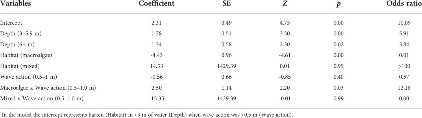
Table 2 Results from logistic regression assessing the probability of successfully stitching a section of photomosaic at different depths, within different habitat types and under differing wave conditions.

We found that failed image alignment was the primary cause of poor stitching success of kelp in deeper water. Image alignment, the first step of the SfM reconstruction process, requires the precise 3D coordinates for a feature (e.g. a corner or edge) to be calculated across multiple overlapping images (Sieberth et al., 2014). A lack of accurately mapped features may result in the failure to correctly align subsequent images, limiting image reconstruction. In very shallow water, failed image alignment also contributed to the poor stitching success of areas of both mixed and macroalgae; however, the impracticality of capturing imagery in very shallow water meant that in some instances imagery from the upper extent of a transect was simply not available for alignment and subsequent stitching.

Macroalgae canopy cover could be evaluated for all virtual quadrats (Table 1). In contrast, benthic community composition could only be calculated for an average of 84 ± 4% of virtual quadrats on each transect (Table 1), which varied between sites. For Leigh and Ōtata, the average number of quadrats where benthic community composition could be determined be made was above 90%. Virtual quadrats that could not be assessed were those with high (> 50%) macroalgae canopy cover. Consequently, not enough points were classified as a benthic community composition type. For Hauturu-o-Toi, the average number of virtual quadrats able to be assessed for benthic community composition was noticeably lower (64 ± 7%.) While high macroalgae canopy cover limited assessment for some quadrats, the primary cause of low benthic assessment rates was due to a filamentous algae bloom. It was extremely difficult to accurately quantify benthic community composition types in both methodological approaches where high densities of overlying filamentous algae were present.

3.2 Data collection

Photogrammetry data collection was faster than field quadrat data collection at Ōtata and Leigh but not Hauturu-o-Toi (Figure 3A, Table 3A). On average ( ± SE) traditional field quadrat data collection took 4.7 ± 1.9 min/quadrat while photogrammetric data collection took 3.1 ± 0.1 min/quadrat, approximately 1 minute and 44 seconds faster per quadrat. Time spent in the field accounted for 100% of the total data collection time for field quadrats, whereas field time only accounted for ~10% of the total data collection time for the photogrammetry method (Figure 3B). This equated to roughly 5 – 6 minutes of time collecting the required imagery per transect or ~19 sec/quadrat.

FIGURE 3

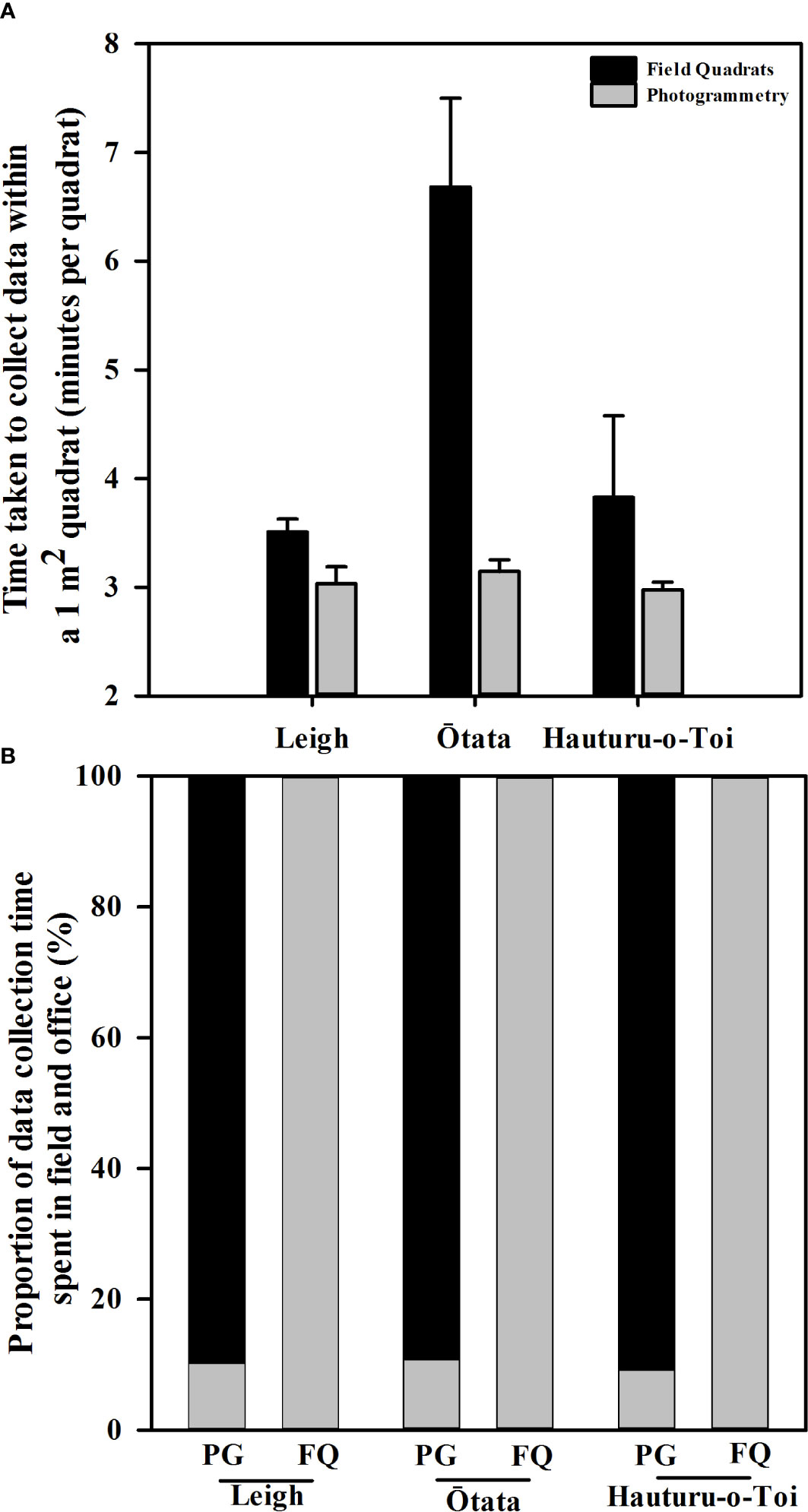
Figure 3 (A) Mean (+ SE) time taken per 1m² quadrat to collect data from virtual photogrammetry quadrats (grey bars) and in situ field quadrats (black bars) at each of the three monitoring sites. (B) Proportion of total data collection time spent in the field (grey bars) and in the office (black bars) for virtual photogrammetry quadrats (PG) and field quadrat (FQ) at each of the three monitoring sites.

TABLE 3

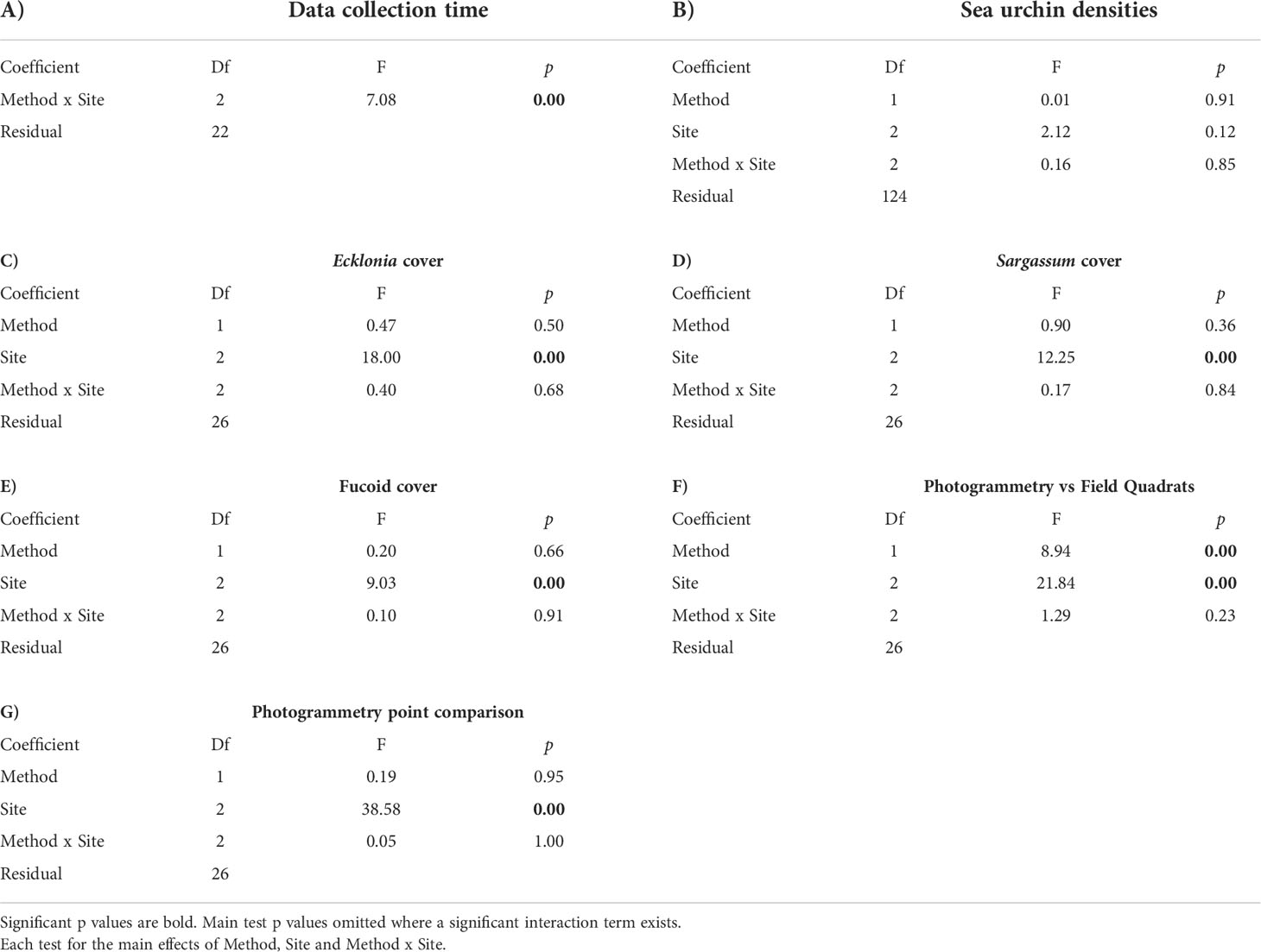
Table 3 Results of two-way ANOVA tests on (A) data collection time, (B) sea urchin densities, (C) canopy cover of Ecklonia radiata and, (D) canopy cover of Sargassum sinclairii, (E) a univariate PERMANOVA test on canopy cover of fucoid algae, (F) a multivariate PERMANOVA test on the difference between photogrammetry and field quadrats, and (G) a multivariate PERMANOVA test on the difference in substratum covers between 25 and 15 random points.

3.3 Sea urchin densities

Mean sea urchin densities did not differ significantly between data collection methodologies, nor was there an interaction between methodology and site (Figure 4A, Table 3B). However, at Leigh, the photomosaics showed non-significant lower densities of sea urchins. This was likely due to higher densities of small (<40 mm test diameter) cryptic sea urchins that were harder to detect within the mosaic.

FIGURE 4

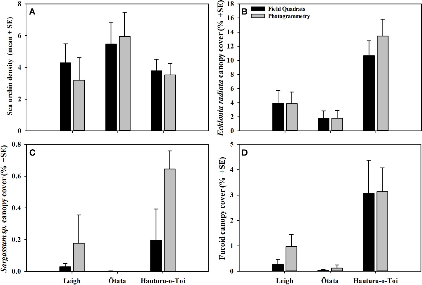
Figure 4 (A) Mean (+SE) sea urchin density, (B) mean Ecklonia radiata canopy cover, (C) mean Sargassum sinclairii canopy cover and (D) mean fucoid canopy cover recorded in virtual photogrammetry quadrats (grey) and field quadrats (black) at each of the three monitoring sites.

3.4 Macroalgae cover

Mean canopy cover for all macroalgae groups (Ecklonia radiata, Sargassum sinclairii and fucoids) did not differ significantly between data collection methodologies nor were there interactions between methodology and site (Figures 4B–D, Tables 3C–E).

3.5 Benthic community composition

Results from the multivariate PERMANOVA showed a difference in benthic community composition between the two methodological approaches (Table 3F). SIMPER analysis found that at all sites sediment cover was a primary contributor to the observed methodological differences and that broadly consistent benthic community compositions, with low levels of average dissimilarity, were recorded between the methods (Figure 5, Table 4). At Leigh and Hauturu-o-Toi sediment was the greatest contributor to overall dissimilarity; sediment cover was four to five times higher within field quadrats than in virtual quadrats. This is highlighted in the nMDS plots for both sites where there is clear separation between the methodologies in the direction of sediment (Figure 6). At Ōtata, recorded sediment cover was approximately three times higher within field quadrats than in virtual photogrammetry plots; however, recorded brown encrusting algae (BEA) cover was approximately four times higher in the virtual photogrammetry quadrats than in the field quadrats (Figure 5). Both contribute equally to overall dissimilarity and nMDS plots show methodological separation, primarily in the direction of sediment/BEA (Figure 6).

TABLE 4

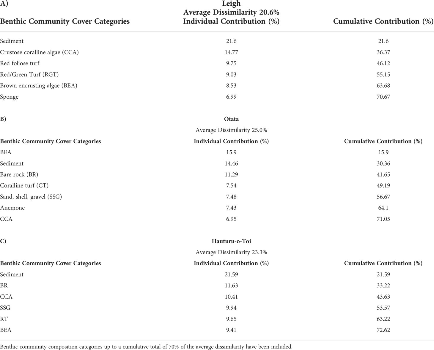
Table 4 SIMPER analysis results at (A) Leigh, (B) Ōtata and (C) Hauturu-o-Toi showing average site dissimilarity between data collection methods (photogrammetry, field quadrats) and key benthic community composition categories contributing towards overall dissimilarity.

FIGURE 5

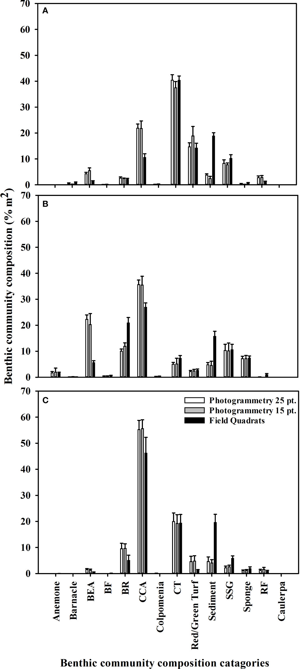
Figure 5 Mean (+SE) benthic community composition percentage covers recorded at (A) Leigh, (B), Ōtata and (C) Hauturu-o-Toi using virtual photogrammetry quadrats with 25 random points (white), virtual photogrammetry quadrats with 15 random points (grey) and field quadrats (black). For display purposes only benthic community composition categories with a mean cover greater than 1% are included.

FIGURE 6

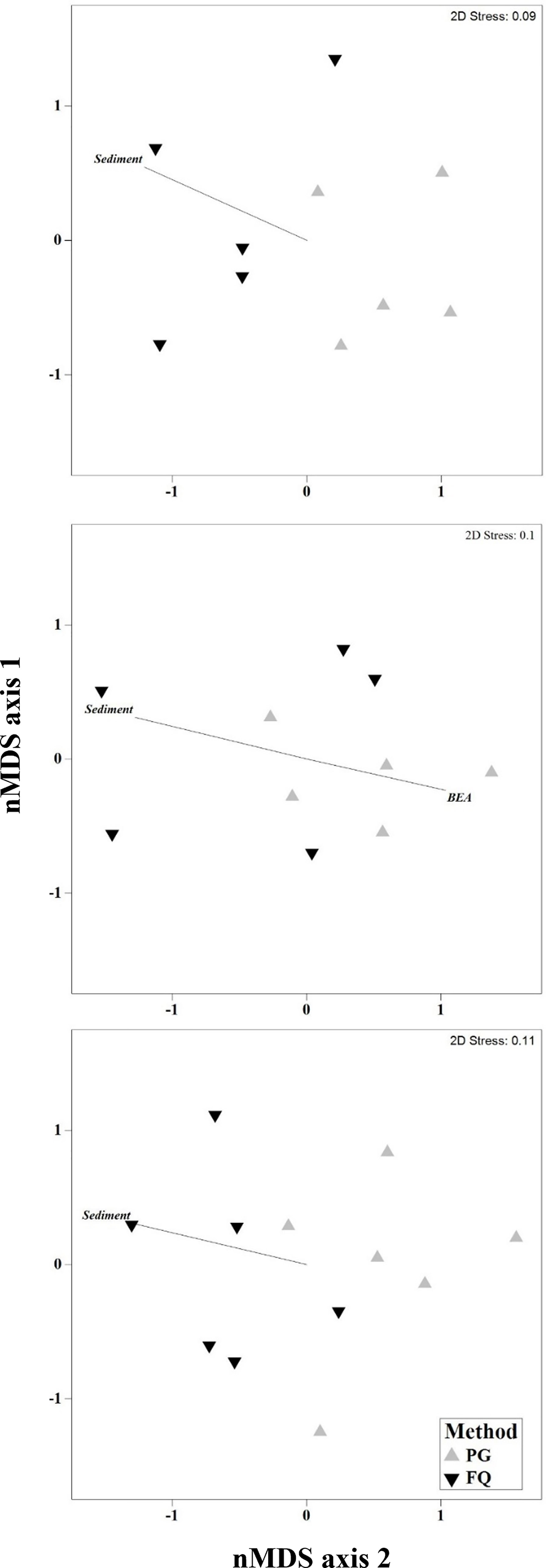
Figure 6 Non-metric multidimensional scaling (nMDS) plots of dominant benthic community composition categories at (A) Leigh, (B) Ōtata and (C) Hauturu-o-Toi as recorded within virtual photogrammetry quadrats (PG, grey) and field quadrats (FQ, black). nMDS plots based on Bray-Curtis distance matrices constructed from square-root transformed transect centroid data. Black lines show directional influence of key benthic community composition categories from SIMPER analysis.

Within virtual quadrats for the photomosaics, we found that the use of 25 random points per quadrat did not yield significantly different overall substratum coverage percentages than 15 random points per quadrat, nor was there any interaction between the number of points and sites surveyed (Figure 5, Table 3G).

4 Discussion

In this study we compared commonly used ecosystem monitoring metrics on temperate rocky reefs dominated by urchin barrens between data extracted from high-resolution, SfM derived, photomosaics and traditional diver-based field quadrats. Primary survey metrics, including sea urchin densities, kelp canopy cover and benthic community composition data, were similar between the two methodologies, consistent with other papers comparing benthic data collected by photography with traditional methods (Dodge et al., 1982; Preskitt et al., 2004; Parravicini et al., 2009; Jokiel et al., 2015) and more specifically comparing the use of photomosaics with traditional methods (Ling, et al., 2016; Raoult et al., 2016; Burns et al., 2020; Barrera-Falcon et al., 2021; Couch et al., 2021). Photogrammetric data collection required minimal in-field time, and can increase the potential survey area. However, not all habitats are suitable, as reconstruction success was hindered in areas of very shallow waters and/or areas where high macroalgal canopy cover existed. High macroalgal canopy cover and the presence of seasonal algal growth restricted the ability to extract benthic community composition information from photomosaics. A wider range of data metrics were able to be collected from field quadrats than photomosaics across all habitat surveyed. Overall we found that high resolution photomosaics were a quick, efficent way of collecting robust data on basic moniroting metrics from temperate rocky reefs with low macroalgae canopy cover, whilst also providing a permanent visual record of the site. In areas where macroalgae cover was high, traditional diver-based field quadrat surveys yielded more comprehensive data as sampling under the canopy remained possible, whereas photomosaics only provided information on macroalgae canopy cover. Decisions regarding the level of detail, and consequently time and resources required for in-field data collection, will ultimately depend on the aims of any study. The strengths and limitations of photomosaics as a tool for monitoring temperate rocky reef ecosystems are discussed below (Table 5).

TABLE 5

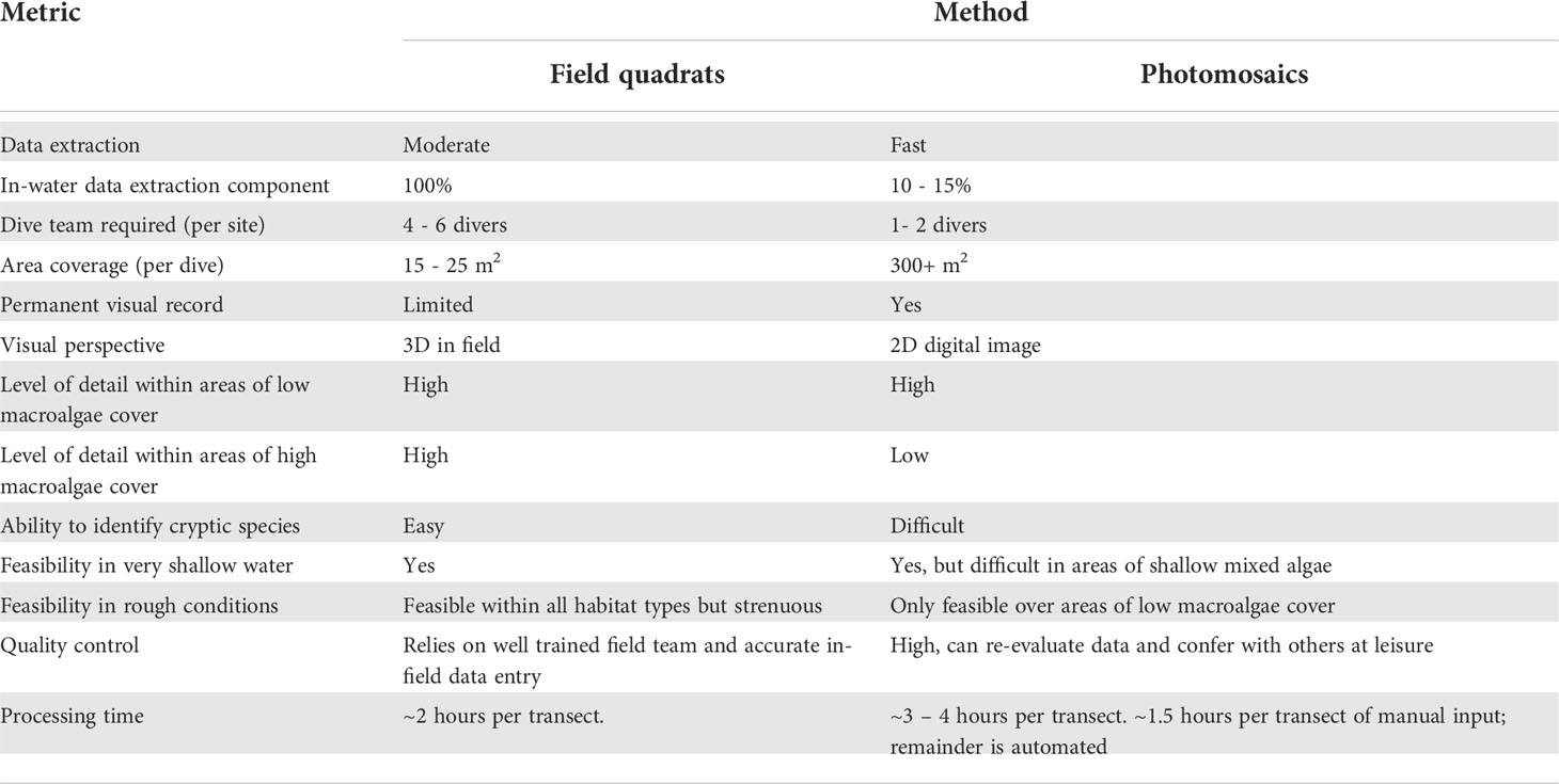
Table 5 Comparative strength and weaknesses of field quadrats and photomosaics within temperate rocky reef ecosystems.

4.1 Strengths and limitations

Data collection from SfM derived photomosaics was generally more time efficient than in-water monitoring using field quadrats. It should however be noted that more data metrics were able to be recorded (and were recorded in this study) within field quadrats than photomosaics, such as specific measurements and invertebrate records. Although this additional data was not considered in the time analysis, some metrics such as recording kelp abundance can be time consuming, and would further increase the overall time taken per field quadrat. The amount of time required for these metrics varied greatly depending on density of invertebrates, macroalgae, etc., but was estimated at roughly 10-20% additional time. Within urchin barrens, where this comparison was primarily conducted and where macroalgae was absent or sparse, the additional time required to make algal and invertebrate measurements was minimal. In this study, where four to six divers conducting multiple dives were required to collect the field quadrat data at each site, a single diver could capture the required photogrammetric imagery within two dives. Importantly, SfM methodolgy conferred the additional advantage of only one tenth of the total data collection time occuring underwater. Monfort et al. (2021) discussed similar findings where rugosity measured from SfM derived 3D point clouds was quicker than in situ ‘chain and tape’ measurements, while Couch et al. (2021) found that photomosaics yeilded similar coral colony data to in situ data collection, but reduced field time by 55%. This reduction in field time is consistent with the use of other photographic techniques, such as photo-quadrats, over field quadrats (Preskitt et al., 2004). Using SfM photogrammetry can significantly reduce the field time and resources required to collect benthic monitoring data and thus can capture more data spatially, albiet from a more limited range of data metrics, in restricted field seasons or windows. While capturing photographic data requires the additional expenses of camera equipment, a number of studies have found that low cost cameras performs well for creating photomosaics (Raoult et al., 2016; Neyer et al., 2019; Nocerino et al., 2019) and that initial costs associated with purchasing equipment are quickly offset by the cost-savings made from reduced field and resources requirements (Jokiel et al., 2015).

The consistency between data collected from the two methods suggests both provide robust forms of benthic monitoring data for key metrics. We did, however, find two notable differences in the datasets. Firstly, sediment cover was consistently higher in field quadrats than in the photomosaic data. This was largely due to different methods for benthic community composition estimates: visual (for field quadrats) and point count (photomosaic) estimates. Visual estimates tease out sediment bound within other substrate types, increasing sediment cover while decreasing other cover types (particularly encrusting and turfing algae). In the point count method, only points where a substrate type could not be identified due overlying sediment were recorded as sediment, resulting in lower sediment estimates. Secondly, brown encrusting algae cover (BEA) was consistently higher in photomosaics at Ōtata. Larger field teams require more training and increase the risk of inter-observer variation and errors. Surveyor experience can play an important role in the quality of collected data (Bernard et al., 2013) and an individuals interpretation of a given classification type, can result in substantial differences from one recorder to another (Cherrill and McClean, 1999; Beijbom et al., 2015). Observer error was considered the likely cause for this differences in BEA cover at Ōtata. Many encrusting algae look superficially similar and different interpretation of BEA between divers may have resulted in misclassificaion. This would result in consistency issues when trying to compare results with future monitoring data. In contrast, extracting data from the photomosaics required a single desk-based annotator who could rest when fatigued, could revisit sections of the imagery if discrepancies were picked up, and could confer with other ecologists for identification, reducing overall error and increasing quality control.

With SfM photogrammetry, a significant time investment is required to process the imagery into usable formats such as photomosaics (Couch et al., 2021). However, once processed, a photomosaic represents a permanent visual archive of a study area that can be repeatedly returned to without the need for further field time. It also allows for a significantly greater area of reef to be surveyed. Where 15 – 20 m² of data was collected from a transect using field quadrats as much as 100 m² was available for data extraction from the photomosaics. These benefits need to be carefully considered against the costs associated with the lengthy processing times required to create these and other SfM outputs. In this study photomosaic processing time was roughly 3 – 4 hours per transect. We did not include photomosaic processing as part of the ‘timed’ data collection because processing timeframes can vary signficantly with image resolution, the number of images being processed and available computing power (Bayley and Mogg, 2020; Couch et al., 2021). Overall processing time will increase with image resolution, larger areas, number of images and less computing power. However, much of the process is fully automated, with batch processing allowing simultaneous processing requiring only periodic manual intervention. For this study the manual processing components included image georeferencing and white balancing, intial workflow set up within Metashape and scaling/refining the sparse cloud. The time taken for this was relatively consistent across transects (~1.5 hours) and accounted for at most 50% of the total photomosaic processing time. In contrast, data recorded from field quadrats does not require computer-orientated post processing but does require transcription into a digital format for analysis. For this study this included copying field data into a digital spreadsheet, labelling and validating photos for each quadrat and data quality checks. This can be slowed or compromised by transcription errors, illegible handwriting or reliance on individuals recollections if data does not make sense. As with photomosaic processing we did not include this transcription into the ‘timed’ data collection processed however this accounted for roughly 2 hours per transect. While overall photomosaic processing time was approximately twice as long as the field quadrat data transcription process, the manual processing time was similar for both methods. Thus, we constrained the activities for time comparison to include data collection only (field and data extraction).

The number of sampling points within a given area can affect both precision and sampling time. We found that reducing the number of sampled points from 25 to 15 did not alter the overall breakdown of substratum covers within a 1 m² quadrat but decreases the time required to analyse a virtual quadrat. Perkins et al. (2016) found the precision of targeted monitoring species, when analysing benthic imagery, was increased by increasing the number of images sampled, as opposed to increasing sampling rate within images. However, the appropriate number of points per unit area will depend on the distribution and abundance of the species of interest (Pante and Dustan, 2012). For comparitive purposes this study only examined point count data within 1 m² quadrats, however the methodological approaches for data extraction from photomosaics are highly varied. In the case of community composition data, this could have also been collected across the length of our transects by hand-drawing polygons around various community catagories (Urbina-Barreto et al., 2021), or with the aid of machine learning classification algorithms (Mohamed et al., 2020; Ternon et al., 2022). This affords researchers the choice of selecting different data extraction method to best meet study aims as well as the ability to use the same underlying data set, but different methodological approaches for data extraction if new questions arise.

Despite increased sampling availabilty within a given photomosaic, reconstructing the entire transect was not always possible. Coverage in the shallowest areas (<1.5 m) was often impractical, while areas of dense macroalgae (typically the upper and lower extents of a transect) suffered from image alignment issues. Image misalignment was likely caused by macroalagal movement between images due to wave action and/or because dense macroalgae represents a homogenous, low contrast surface where the feature matching algorithms failed to pick out distinct points (Mancini et al., 2013). Vegetation movement, caused by high wind speeds, can cause feature mismatches and poor image alignment in UAV forest surveys (Dandois et al., 2015; Fraser and Congalton, 2018). Similarly, water motion can cause macroalgal movement between images, also resulting in feature mismatches and a failure to properly align images. In terrestrial systems, these alignment issues can be overcome by flying at greater altitiudes (Fraser and Congalton, 2018), which increases the area available in each image to detect features and reduces perspective distortion between images. We recommend that underwater imagery for SfM processing over macroalgae be captured at least 1 m above the benthos to improve the chances of success. Alternatively, issues matching homogeneous, low contrast features might explain why images over dense monospecific stands of macroalgae failed to align while areas along the same transect, surveyed under the same sea state conditions and dominated by a mixture of dense turfing and foliosed algae along with juvenile macroalgae, were able to be aligned. Overall, we found photomosaics provided limited monitoring information over areas of dense macroalgae cover.

Dense macroalgal canopies conceal underlying substratum, thereby reducing the utility of the imagery for substratum assessment (Tait et al., 2019). Where field quadrats can access under the kelp canopy and collect underlying benthic data, the photomosaics were only able to provide basic macroalgae canopy cover data. Seasonal filamentous algal blooms also caused data collection issues for photogrammetry and to a lesser extent for field quadrats. Where possible, imagery collections should occur outside of key growth periods for filamentous algae. Although not a major issue for this study, 2D imagery, such as photomosaics and photo-quadrats, are limited in their ability to detect organisms or substrate types occupying in deep cracks or overhangs (Jokiel et al., 2015; Couch et al., 2021). We found that photomosaics were less able to detect small sea urchins (<40 mm) hidden in cracks and crevices. Similarly, Ling et al. (2016) found that daytime density estimates of the sea urchin Centrostephanus rodgersii, which preferentially occupy crevices during the day, were lower in photomosaics than estimates from divers who were able to inspect crevices as they surveyed the area. While this study was designed to investigate data captured from 2D photomosaics, three-dimensional forms of photogrammetry data, such as point clouds and 3D meshes, may be able to be utilised to gather additional data from highly complexity reefs.

It has been suggested in tropical systems that there is unlikely to be a single method that can be considered the ‘gold standard’ for benthic monitoring (Burns et al., 2020; Couch et al., 2021). This appears true within temperate rocky reef ecosystems as well. As SfM derived photogrammetry has increased in popularity, and data derived from photogrammetry can be standardised with that collected from more traditional means (Jokiel et al., 2015), researchers have the ability to select and develop monitoring approaches that draw upon the strengths of different combinations of traditional and emerging techniques. For example, a study could incorporate field quadrat-based approaches in very shallow or highly layered habitats but using SfM photogrammetry in areas with low macroalgal cover, or a broad-scale SfM photogrammetry across a large area with fine detail collected from a smaller number of field quadrats. The ability to use diverse and perhaps complementary techniques will allow benthic ecologists to maximise data collection across the spectrum of habitat types present throughout an ecosystem within realistic time and resource constraints.

5 Conclusion

The results from this study build our understanding of the strengths and weakness of utilising diver-generated photomosaics, a form of SfM derived photogrammetry, for monitoring temperate rocky reefs. Photomosaics provide robust, spatially extensive data for a number of key rocky reef metrics, but is limited with respect to cryptic or understory species. Photogrammetry data collection is generally more time efficient than in situ field quadrat monitoring and requires minimal dive time. It also provides a permanent record of a site which can be reinvestigated without more time in the field. Their utility is lessened in areas of high macroalgae canopy cover, very shallow water or heightened sea state. Thus diver-generated photomosaics are a valuable monitoring tool in areas of low macroalgae cover, such as urchin barrens, but of limited value within kelp forests. As with comparative studies in tropical systems, highlighting the strengths and weakness of different data collectiong methodolgies reveals there is unlikely to be a ‘gold standard’ for monitoring temperate rocky reef ecosystems. Instead developing flexible monitoring programmes that utilise a range of techniques, including photogrammetry and more traditional methods, will result in the greatest level of data capture and spatial coverage, while reducing in-field resource and time related costs.

Data availability statement

The datasets presented in this study can be found in online repositories. The names of the repository/repositories and accession number(s) can be found below: https://figshare.com/projects/Divergenerated_photomosaics_as_a_tool_for_monitoring_temperate_rocky_reef_ecosystems/140110.

Author contributions

AS and KM conceived the ideas and designed methodology. AS and KM collected the data. AS analysed the data. AS led the writing of the manuscript. All authors contributed critically to the drafts and gave final approval for publication.

Funding

Funding for this project was provided by Live Ocean Charitable Trust, New Zealand Geographic, Foundation North: GIFT, and University of Auckland Doctoral Scholarship (awarded to KM).

Acknowledgments

Thanks to James Frankham for ongoing encouragement and support for the project; thanks to staff and students at the Leigh Marine Laboratory for assistance with field work. Thanks to two reviewers for their helpful feedback and improvements to this manuscript.

Conflict of interest

The authors declare that the research was conducted in the absence of any commercial or financial relationships that could be construed as a potential conflict of interest.

Publisher’s note

All claims expressed in this article are solely those of the authors and do not necessarily represent those of their affiliated organizations, or those of the publisher, the editors and the reviewers. Any product that may be evaluated in this article, or claim that may be made by its manufacturer, is not guaranteed or endorsed by the publisher.

Supplementary material

The Supplementary Material for this article can be found online at: https://www.frontiersin.org/articles/10.3389/fmars.2022.953191/full#supplementary-material

References

Anderson M. J. (2014). Permutational multivariate analysis of variance (PERMANOVA) (John wiley & sons, Inc. Hoboken, New Jersey: Wiley statsref: statistics reference online), 1–15.

Google Scholar

Aplin P. (2005). Remote sensing: ecology. Prog. Phys. Geogr. 29, 104–113. doi: 10.1191/030913305pp437pr

CrossRef Full Text | Google Scholar

Barrera-Falcon E., Rioja-Nieto R., Hernández-Landa R. C., Torres-Irineo E. (2021). Comparison of standard Caribbean coral reef monitoring protocols and underwater digital photogrammetry to characterize hard coral species composition, abundance, and cover. Front. Mar. Sci. 8, 722569. doi: 10.3389/fmars.2021.722569

CrossRef Full Text | Google Scholar

Bayley D., Mogg A. (2020). A protocol for the large-scale analysis of reefs using structure from motion photogrammetry. Methods Ecol. Evol. 11, 1410–1420. doi: 10.1111/2041-210X.13476

CrossRef Full Text | Google Scholar

Bayley D. T., Mogg A. O., Koldewey H., Purvis A. (2019). Capturing complexity: field-testing the use of ‘structure from motion' derived virtual models to replicate standard measures of reef physical structure. PeerJ 7, e6540. doi: 10.7717/peerj.6540

PubMed Abstract | CrossRef Full Text | Google Scholar

Beijbom O., Edmunds P., Roelfsema C., Smith J., Kline D., Neal B., et al. (2015). Towards automated annotation of benthic survey images: Variability of human experts and operational modes of automation. PLoS One 10, e0130312. doi: 10.1371/journal.pone.0130312

PubMed Abstract | CrossRef Full Text | Google Scholar

Bennion M., Fisher J., Yesson C., Brodie J. (2019). Remote sensing of kelp (Laminariales, ochrophyta): monitoring tools and implications for wild harvesting. Rev. Fish. Sci. Aquacult. 27, 127–141. doi: 10.1080/23308249.2018.1509056

CrossRef Full Text | Google Scholar

Bernard A. T., Götz A., Kerwath S. E., Wilke C. G. (2013). Observer bias and detection probability in underwater visual census of fish assemblages measured with independent double-observers. J. Exp. Mar. Biol. Ecol. 433, 75–84. doi: 10.1016/j.jembe.2013.02.039

CrossRef Full Text | Google Scholar

Bohnsack J. A. (1979). Photographic quantitative sampling of hard-bottom benthic communities. Bull. Mar. Sci. 29, 242–252.

Google Scholar

Braunisch V., Suchant R. (2010). Predicting species distributions based on incomplete survey data: the trade-off between precision and scale. Ecography 33, 826–840. doi: 10.1111/j.1600-0587.2009.05891.x

CrossRef Full Text | Google Scholar

Burns J. H., Delparte D., Gates R. D., Takabayashi M. (2015). Integrating structure-from-motion photogrammetry with geospatial software as a novel technique for quantifying 3D ecological characteristics of coral reefs. PeerJ 3, e1077. doi: 10.7717/peerj.1077

PubMed Abstract | CrossRef Full Text | Google Scholar

Burns J., Weyenberg G., Mandel T., Ferreira S., Gotshalk D., Kinoshita C., et al. (2020). A comparison of the diagnostic accuracy of in situ and digital image-based assessments of coral health and disease. Front. Mar. Sci. 7, 304. doi: 10.3389/fmars.2020.00304

CrossRef Full Text | Google Scholar

Casella E., Collin A., Harris D., Ferse S., Bejarano S., Parravicini V., et al. (2017). Mapping coral reefs using consumer-grade drones and structure from motion photogrammetry techniques. Coral Reefs 36, 269–275. doi: 10.1007/s00338-016-1522-0

CrossRef Full Text | Google Scholar

Cavanaugh K. C., Cavanaugh K. C., Bell T. W., Hockridge E. G. (2021). An automated method for mapping giant kelp canopy dynamics from UAV. Front. Environ. Sci. 8, 58735. doi: 10.3389/fenvs.2020.587354

CrossRef Full Text | Google Scholar

Cherrill A., McClean C. (1999). The reliability of ‘Phase 1’habitat mapping in the UK: the extent and types of observer bias. Landscape urban Plann. 45, 131–143. doi: 10.1016/S0169-2046(99)00027-4

CrossRef Full Text | Google Scholar

Clarke K. R., Gorley R. N., Somerfield P. J., Warwick R. M. (2014). Change in marine communities: an approach to statistical analysis and interpretation, 3rd edition (Plymouth: PRIMER-E).

Google Scholar

Couch C., Oliver T., Suka R., Lamirand M., Asbury M., Amir C., et al. (2021). Comparing coral colony surveys from in-water observations and structure-from-Motion imagery shows low methodological bias. Front. Mar. Science. 8, 657943. doi: 10.3389/fmars.2021.647943

CrossRef Full Text | Google Scholar

D'Urban Jackson T., Williams G. J., Walker-Springett G., Davies A. J. (2020). Three-dimensional digital mapping of ecosystems: a new era in spatial ecology. Proc. R. Soc. B 287, 20192383. doi: 10.1098/rspb.2019.2383

CrossRef Full Text | Google Scholar

Dandois J. P., Olano M., Ellis E. C. (2015). Optimal altitude, overlap, and weather conditions for computer vision UAV estimates of forest structure. Remote Sens. 7, 13895–13920. doi: 10.3390/rs71013895

CrossRef Full Text | Google Scholar

Del Vecchio S., Fantinato E., Silan G., Buffa G. (2019). Trade-offs between sampling effort and data quality in habitat monitoring. Biodiv. Conserv. 28, 55–73. doi: 10.1007/s10531-018-1636-5

CrossRef Full Text | Google Scholar

De Oliveira L. M. C., Lim A., Conti L. A., Wheeler A. J. (2021). 3D classification of cold-water coral reefs: A comparison of classification techniques for 3D reconstructions of cold-water coral reefs and seabed. Front. Mar. Sci. 8, 640713. doi: 10.3389/fmars.2021.640713

CrossRef Full Text | Google Scholar

Dodge R. E., Logan A., Antonius A. (1982). Quantitative reef assessment studies in Bermuda: a comparison of methods and preliminary results. Bull. Mar. Sci. 32, 745–760.

Google Scholar

Fakiris E., Papatheodorou G., Kordella S., Christodoulou D., Galgani F., Geraga M. (2022). Insights into seafloor litter spatiotemporal dynamics in urbanized shallow Mediterranean bays. an optimized monitoring protocol using towed underwater cameras. J. Environ. Manage. 308, 114647. doi: 10.1016/j.jenvman.2022.114647

PubMed Abstract | CrossRef Full Text | Google Scholar

Francis R. I. C. C., McKenzie J. R. (2015). “Assessment of the SNA 1 stocks in 2013,” in New Zealand fisheries assessment report 2015/76, (Wellington, New Zealand: Ministry of Primary Industries) 82 p.

Google Scholar

Fraser B. T., Congalton R. G. (2018). Issues in unmanned aerial systems (UAS) data collection of complex forest environments. Remote Sens. 10, 908. doi: 10.3390/rs10060908

CrossRef Full Text | Google Scholar

Halpern B., Frazier M., Afflerbach J., Lowndes J., Micheli F., O’Hara C., et al. (2019). Recent pace of change in human impact on the world’s ocean. Sci. Rep. 9, 1–8. doi: 10.1038/s41598-019-47201-9

PubMed Abstract | CrossRef Full Text | Google Scholar

Halpern B. S., Walbridge S., Selkoe K. A., Kappel C. V., Micheli F., D'Agrosa C., et al. (2008). A global map of human impact on marine ecosystems. Science 319, 948–952. doi: 10.1126/science.1149345

PubMed Abstract | CrossRef Full Text | Google Scholar

Jokiel P. L., Rodgers K. S., Brown E. K., Kenyon J. C., Aeby G., Smith W. R., et al. (2015). Comparison of methods used to estimate coral cover in the Hawaiian islands. PeerJ 3, e954. doi: 10.7717/peerj.954

PubMed Abstract | CrossRef Full Text | Google Scholar

Klemas V. V. (2015). Coastal and environmental remote sensing from unmanned aerial vehicles: An overview. J. Coast. Res. 35, 1260–1267. doi: 10.2112/JCOASTRES-D-15-00005.1

CrossRef Full Text | Google Scholar

Kohler K. E., Gill S. M. (2006). Coral point count with excel extensions (CPCe): A visual basic program for the determination of coral and substrate coverage using random point count methodology. Comput. geosci. 32, 1259–1269. doi: 10.1016/j.cageo.2005.11.009

CrossRef Full Text | Google Scholar

Lindenmayer D. B., Likens G. E. (2010). The science and application of ecological monitoring. Biol. Conserv. 143, 1317–1328. doi: 10.1016/j.biocon.2010.02.013

CrossRef Full Text | Google Scholar

Ling S. D., Mahon I., Marzloff M. P., Pizarro O., Johnson C. R., Williams S. B. (2016). Stereo-imaging AUV detects trends in sea urchin abundance on deep overgrazed reefs. Limnol. Oceanogr.: Methods 14, 293–304. doi: 10.1002/lom3.10089

CrossRef Full Text | Google Scholar

Lochhead I., Hedley N. (2022). Evaluating the 3D integrity of underwater structure from motion workflows. Photogrammetr. Rec. doi: 10.1111/phor.12399

CrossRef Full Text | Google Scholar

Logan A., Page F. H., Thomas M. L. (1984). Depth zonation of epibenthos on sublittoral hard substrates off deer island, bay of fundy, Canada. Estuarine Coast. Shelf Sci. 18, 571–592. doi: 10.1016/0272-7714(84)90091-X

CrossRef Full Text | Google Scholar

Lovett G., Burns D., Driscoll C., Jenkins J., Mitchell M., Rustad L., et al. (2007). Who needs environmental monitoring? Front. Ecol. Environ. 5, 253–260. doi: 10.1890/1540-9295(2007)5[253:WNEM]2.0.CO;2

CrossRef Full Text | Google Scholar

Mancini F., Dubbini M., Gattelli M., Stecchi F., Fabbri S., Gabbianelli G. (2013). Using unmanned aerial vehicles (UAV) for high-resolution reconstruction of topography: The structure from motion approach on coastal environments. Remote Sens. 5, 6880–6898. doi: 10.3390/rs5126880

CrossRef Full Text | Google Scholar

Marre G., Deter J., Holon F., Boissery P., Luque S. (2020). Fine-scale automatic mapping of living posidonia oceanica seagrass beds with underwater photogrammetry. Mar. Ecol. Prog. Ser. 643, 63–74. doi: 10.3354/meps13338

CrossRef Full Text | Google Scholar

Marre G., Holon F., Luque S., Boissery P., Deter J. (2019). Monitoring marine habitats with photogrammetry: a cost-effective, accurate, precise and high-resolution reconstruction method. Front. Mar. Sci. 6, 276. doi: 10.3389/fmars.2019.00276

CrossRef Full Text | Google Scholar

Mihoub J. B., Henle K., Titeux N., Brotons L., Brummitt N. A., Schmeller D. S. (2017). Setting temporal baselines for biodiversity: the limits of available monitoring data for capturing the full impact of anthropogenic pressures. Sci. Rep. 7, 1–13. doi: 10.1038/srep41591

PubMed Abstract | CrossRef Full Text | Google Scholar

Mizuno K., Asada A., Matsumoto Y., Sugimoto K., Fujii T., Yamamuro M., et al. (2017). A simple and efficient method for making a high-resolution seagrass map and quantification of dugong feeding trail distribution: A field test at Mayo bay, Philippines. Ecol. Inf. 38, 89–94. doi: 10.1016/j.ecoinf.2017.02.003

CrossRef Full Text | Google Scholar

Mohamed H., Nadaoka K., Nakamura T. (2020). Towards benthic habitat 3D mapping using machine learning algorithms and structures from motion photogrammetry. Remote Sens. 12, 127. doi: 10.3390/rs12010127

CrossRef Full Text | Google Scholar

Monfort T., Cheminée A., Bianchimani O., Drap P., Puzenat A., Thibaut T. (2021). The three-dimensional structure of Mediterranean shallow rocky reefs: Use of photogrammetry-based descriptors to assess its influence on associated teleost assemblage. Front. Mar. Sci. 8, 924. doi: 10.3389/fmars.2021.639309

CrossRef Full Text | Google Scholar

Neyer F., Nocerino E., Grün A. (2019). Image quality improvements in low-cost underwater photogrammetry. international archives of the photogrammetry. Remote Sens. Spatial Inf. Sci. 42, 135–142. doi: 10.3929/ethz-b-000343605

CrossRef Full Text | Google Scholar

Nocerino E., Menna F., Gruen A., Troyer M., Capra A., Castagnetti C., et al. (2020). Coral reef monitoring by scuba divers using underwater photogrammetry and geodetic surveying. Remote Sens. 12, 3036. doi: 10.3390/rs12183036

CrossRef Full Text | Google Scholar

Nocerino E., Neyer F., Grün A., Troyer M., Menna F., Brooks A., et al. (2019). Comparison of diver-operated underwater photogrammetric systems for coral reef monitoring. SPRS-international archives of the photogrammetry. Remote Sens. Spatial Inf. Sci. XLII-2/W10, 143–150. doi: 10.5194/isprs-archives-XLII-2-W10-143-2019

CrossRef Full Text | Google Scholar

Palma M., Rivas Casado M., Pantaleo U., Pavoni G., Pica D., Cerrano C. (2018). SfM-based method to assess gorgonian forests (Paramuricea clavata (Cnidaria, octocorallia)). Remote Sens. 10, 1154. doi: 10.3390/rs10071154

CrossRef Full Text | Google Scholar

Pante E., Dustan P. (2012). Getting to the point: Accuracy of point count in monitoring ecosystem change. J. Mar. Biol. 2012, 1–7. doi: 10.1155/2012/802875

CrossRef Full Text | Google Scholar

Parravicini V., Morri C., Ciribilli G., Montefalcone M., Albertelli G., Bianchi C. N. (2009). Size matters more than method: visual quadrats vs photography in measuring human impact on Mediterranean rocky reef communities. Estuarine Coast. Shelf Sci. 81, 359–367. doi: 10.1016/j.ecss.2008.11.007

CrossRef Full Text | Google Scholar

Perkins N. R., Foster S. D., Hill N. A., Barrett N. S. (2016). Image subsampling and point scoring approaches for large-scale marine benthic monitoring programs. Estuarine Coast. Shelf Sci. 176, 36–46. doi: 10.1016/j.ecss.2016.04.005

CrossRef Full Text | Google Scholar

Pizarro O., Friedman A., Bryson M., Williams S. B., Madin J. (2017). A simple, fast, and repeatable survey method for underwater visual 3D benthic mapping and monitoring. Ecol. Evol. 7, 1770–1782. doi: 10.1002/ece3.2701

PubMed Abstract | CrossRef Full Text | Google Scholar

Preskitt L. B., Vroom P. S., Smith C. M. (2004). A rapid ecological assessment (REA) quantitative survey method for benthic algae using photoquadrats with scuba. Pacific Sci. 58, 201–209. doi: 10.1353/psc.2004.0021

CrossRef Full Text | Google Scholar

Raoult V., David P. A., Dupont S. F., Mathewson C. P., O’Neill S. J., Powell N. N., et al. (2016). GoPros™ as an underwater photogrammetry tool for citizen science. PeerJ 4, e1960. doi: 10.7717/peerj.1960

PubMed Abstract | CrossRef Full Text | Google Scholar

Roberts D. E., Fitzhenry S. R., Kennelly S. J. (1994). Quantifying subtidal macrobenthic assemblages on hard substrata using a jump camera method. J. Exp. Mar. Biol. Ecol. 177, 157–170. doi: 10.1016/0022-0981(94)90234-8

CrossRef Full Text | Google Scholar

Seers B. M., Shears N. T. (2015). Spatio-temporal patterns in coastal turbidity–long-term trends and drivers of variation across an estuarine-open coast gradient. Estuarine Coast. Shelf Sci. 154, 137–151. doi: 10.1016/j.ecss.2014.12.018

CrossRef Full Text | Google Scholar

Shears N. T., Babcock R. C. (2002). Marine reserves demonstrate top-down control of community structure on temperate reefs. Oecologia 132, 131–142. doi: 10.1007/s00442-002-0920-x

PubMed Abstract | CrossRef Full Text | Google Scholar

Shears N. T., Babcock C. R. (2004). Community composition and structure of shallow subtidal reefs in northeastern new Zealand (Wellington, New Zealand: Department of Conservation).

Google Scholar

Sieberth T., Wackrow R., Chandler J. H. (2014). Influence of blur on feature matchin and a geometric approach for photogrammetric deblurring. Int. Arch. Photogrammetr. Remote Sens. Spatial Inf. Sci. XL-3, 321–326. doi: 10.5194/isprsarchives-XL-3-321-2014

CrossRef Full Text | Google Scholar

Smale D. A., Epstein G., Hughes E., Mogg A. O., Moore P. J. (2020). Patterns and drivers of understory macroalgal assemblage structure within subtidal kelp forests. Biodiv. Conserv. 29, 4173–4192. doi: 10.1007/s10531-020-02070-x

CrossRef Full Text | Google Scholar

Solan M., Cardinale B. J., Downing A. L., Engelhardt K. A., Ruesink J. L., Srivastava D. S. (2004). Extinction and ecosystem function in the marine benthos. Science 306, 1177–1180. doi: 10.1126/science.1103960

PubMed Abstract | CrossRef Full Text | Google Scholar

Suka R., Asbury M., Gray A. E., Winston M., Oliver T., Couch C. S. (2019). Processing photomosaic imagery of coral reefs using structure-from-MotionStandard operating procedures (Honolulu: U.S: Department of Commerce, National Oceanic and Atmospheric Administration).

Google Scholar

Tait L., Bind J., Charan-Dixon H., Hawes I., Pirker J., Schiel D. (2019). Unmanned aerial vehicles (UAVs) for monitoring macroalgal biodiversity: comparison of RGB and multispectral imaging sensors for biodiversity assessments. Remote Sens. 11, 2332. doi: 10.3390/rs11192332

CrossRef Full Text | Google Scholar

Teague J., Scott T. (2017). Underwater photogrammetry and 3D reconstruction of submerged objects in shallow environments by ROV and underwater GPS. J. Mar. Sci. Res. Technol. 1, 005.

Google Scholar

Ternon Q., Danet V., Thiriet P., Ysnel F., Feunteun E., Collin A. (2022). Classification of underwater photogrammetry data for temperate benthic rocky reef mapping. Estuarine Coast. Shelf Sci. 270, 107833. doi: 10.1016/j.ecss.2022.107833

CrossRef Full Text | Google Scholar

Urbina-Barreto I., Garnier R., Elise S., Pinel R., Dumas P., Mahamadaly V., et al. (2021). Which method for which purpose? a comparison of line intercept transect and underwater photogrammetry methods for coral reef surveys. Front. Mar. Sci. 8, 636902. doi: 10.3389/fmars.2021.636902

CrossRef Full Text | Google Scholar

Webber D. N., Starr P. J., Haist V., Rudd M., Edwards C. T. T. (2018). “The 2017 stock assessment and management procedure evaluation for rock lobsters (Jasus edwardsii) in CRA 2,” in New Zealand fisheries assessment report 2018/17, 87 p.

Google Scholar

Yao H., Qin R., Chen X. (2019). Unmanned aerial vehicle for remote sensing applications–a review. Remote Sens. 11, 1443. doi: 10.3390/rs11121443

CrossRef Full Text | Google Scholar