Southern Ocean ice charts at the Argentine Naval Hydrographic Service and their impact on safety of navigation

Introduction

Antarctica is strategically valued as a natural laboratory, a reservoir of fresh water, and critical for understanding and monitoring the dynamics of global climate change. It is a continent surrounded by seas influenced by ocean currents, winds, and variations in the concentration and thickness of sea ice, that make it a unique place. Sea ice has a significant impact on climate regulation and the global energy balance. Formation of sea ice occurs when seawater freezes at temperatures of -1.8°C, a salinity of 27 ‰, and with favorable hydro-meteorological conditions for its growth (WMO No. 574, 2021). Sea ice can be found floating adrift on the ocean surface or lying along the coasts, in front of barriers, or surrounding grounded icebergs (WMO No. 259, 2014b).

Logistics and scientific activities in Antarctica are determined by the presence of sea ice and icebergs, making it essential to have the most accurate sea-ice information, allowing the planning of different tasks, and the means to carry out operational activities, such as the use of inflatable and medium-sized boats with landing ramps, or helicopters (Pope et al., 2017). Similarly, tourist activity in Antarctica has been developing since the late 1960s, with a primary focus on attractions in the vicinity of the Antarctic Peninsula and adjacent islands. Last period there was an increase in tourist activity at a rate of 8.6%, with more than 50,000 visitors on more than 50 vessels of different sizes and characteristics during the season October 2018 to March 2019 (International Association of Antarctica Tour Operators, 2020).

The position and drift of icebergs, sea-ice concentration, and extent of the ice field have been monitored using satellite data for decades, yet information on additional parameters such as sea-ice stage of development, thickness and areas of pressure ridging provide a better understanding of ice conditions to support navigational safety for mariners. However, monitoring sea ice and its geophysical parameters is difficult due to differences in snow cover, seasonal variability, vast areas without observations from ships or stations, among others. Additionally to these obstacles, typically only one set of satellite data is available at a given time (i.e. individual polar orbit satellites provides imagery one at a time) and optical data commonly limited by cloud cover and passive microwave data limited by horizontal resolution (Dierking, 2013).

To respond to the requirement of sea-ice monitoring, national ice services develop ice charts that are compiled using an exhaustive set of satellite observations to offer all the available information in a graphical, complete and simplified format. Ice charts are produced by sea-ice analysts following international standards (WMO No. 1215, 2014a) including additional sea-ice parameters and the presence of icebergs, that are not always clearly discernible from satellites. The development of ice charts originated to provide guidance and support to sailors in the Polar Regions, particularly in the Arctic, but also subpolar areas with high maritime traffic, such as the Baltic Sea, Barents Sea, Denmark Strait, Bering Strait, among others (Partington et al., 2003). Ice Services from Canada, Denmark, Finland, Germany, Norway, Russia, Sweden, and the USA, among others, have been developing ice charts for more than 4 decades; while in the Southern Hemisphere the countries that follow the same procedures are limited. These differences are mainly related to the extremely important commercial use of the polar and subpolar sea routes of the Northern Hemisphere where the presence of ice limits navigation with the consequent cost implications for naval transport. In the Southern Hemisphere, Antarctica and adjacent areas of the austral oceans, the greatest commercial activity is related to tourist cruises during the southern spring and summer and a still limited fishing activity. Pope et al. (2017) describe the work of the Ice Services or other National Organizations with ice chart production for the Southern Oceans: Argentina, Australia, Chile, China, Denmark, Germany, Norway, Russia and the USA. These organizations provide different ice chart products based on their mandate, financial capabilities and regions of interest. Common challenges related to limitations of the availability of satellite data also affects these Services.

Ice charts pre-date the satellite age (late 1960’s with the onset of NIMBUS and other single sensor optical satellites), when routine products were produced using aerial reconnaissance, ship-based observations and local knowledge of sea ice areas, particularly closer to the land (Divine and Dick, 2006; Mahoney et al., 2008; Walsh et al., 2017). Since 1972 the U.S. National Ice Center (US NIC) has produced Arctic and Antarctic ice charts for operational purposes, including activity planning and nautical safety. The long consistent archive of operational charts has opened opportunities for numerous research projects that rely on ice chart databases for the validation of sea ice products developed for climate monitoring. For example, Kukla and Robinson (1980) use the ice charts for climatic studies of associated variables such as ice rim position, albedo, and snow depth. Knol et al. (2018) outline challenges in terms of changes in the information infrastructure of Ice Services in the Arctic, describing the different web services to access ice information in the Northern Hemisphere. For example, the Ocean and Sea Ice Satellite Application Facility (OSI SAF) generates derived products from climate records of gridded global ice concentration (Lavergne et al., 2019).

In order to provide ice charts suitable for navigational safety, it is essential to have the most up-to-date information on current sea-ice and iceberg conditions. To access this information during operations, or near real-time, satellite imagery from various sensors is used as the main source and paired with ship-based observations and coastal monitoring stations or aerial reconnaissance. But infrequent point observations have considerable limitations in terms of geographic coverage and frequency of acquisition and are therefore of relatively low importance from an operational point of view (Hall et al., 2002). There has been some development to automate ship-based observations with the use of video cameras. Digital images acquired from the ice condition monitoring video cameras deployed on the NB Palmer icebreaker during the 2007 SIMBA expedition were subjected to modern image analysis techniques to verify and validate ice observationsand provided high temporal resolution of continuous observations, which may eventually be used to validate satellite-derived products, such as ice charts (Weissling et al., 2009). Observations from helicopters and aerial drones have been improving with a significant amount of information including roughness, thickness and concentration (Divine et al., 2016; Li et al., 2019)

In this regard, remotely sensed data, such as satellite images, have become a very valuable tool for Earth observation and have become fundamental to support better decision-making. The interpretation and analysis of the products of these sensors have allowed the planning, execution, monitoring and evaluation of projects to be carried out safe and more efficiently, optimizing resources and their sustainability (Arias Duarte et al., 2010). For this reason, improving the current procedures of how satellites are analyzed is essential for ice services to provide better support in greater detail and precision.

The Argentine Naval Hydrographic Service (Servicio de Hidrografia Naval, SHN) has been supporting Argentine Navy Ships since 1970s, but the ice information has not been publicly available until recently. In 2015, SHN introduced the publication of its ice charts to general maritime users and started working as a recognized National Ice Service (WMO 574 (2021)). SHN’s routine products include the weekly production of ice charts for the Weddell Sea, Bellingshausen Sea and South Atlantic Ocean, iceberg drift charts, and detailed information through the Navtex and SafetyNet services for the safety of navigation.

The objective of this paper is to present the current state of SHN actions related to Ice Service duties, including a description of ice charting procedures, the satellite imagery processing and the analysis of different classes of sea ice and icebergs necessary for operations in Argentina’s area of national responsibility. By giving visibility and clarification on the methods used for the analysis of sea-ice conditions and the presence of icebergs, the end-users can improve in the interpretation of this information for better decision-making in ice infested waters.

Data and methodology

Area of study

This paper is focused on the NAVAREA VI, the Argentine area of responsibility in terms of public service for Safety at Sea (Figure 1). This area includes the Antarctic Peninsula, Bellingshausen Sea, Weddell Sea and the Southwestern Atlantic Ocean. Ice charts are developed for the sub-areas detailed in Figure 2, including Scotia Sea, Weddell Sea and Bellingshausen Sea. Sea ice does not usually extend north of the 60° South latitude (Venegas and Drinkwater, 2001) yet, icebergs drift can extend to subtropical latitudes over the South Atlantic Ocean, thus it is necessary to have a separate iceberg analysis chart that includes all the NAVAREA VI.

FIGURE 1

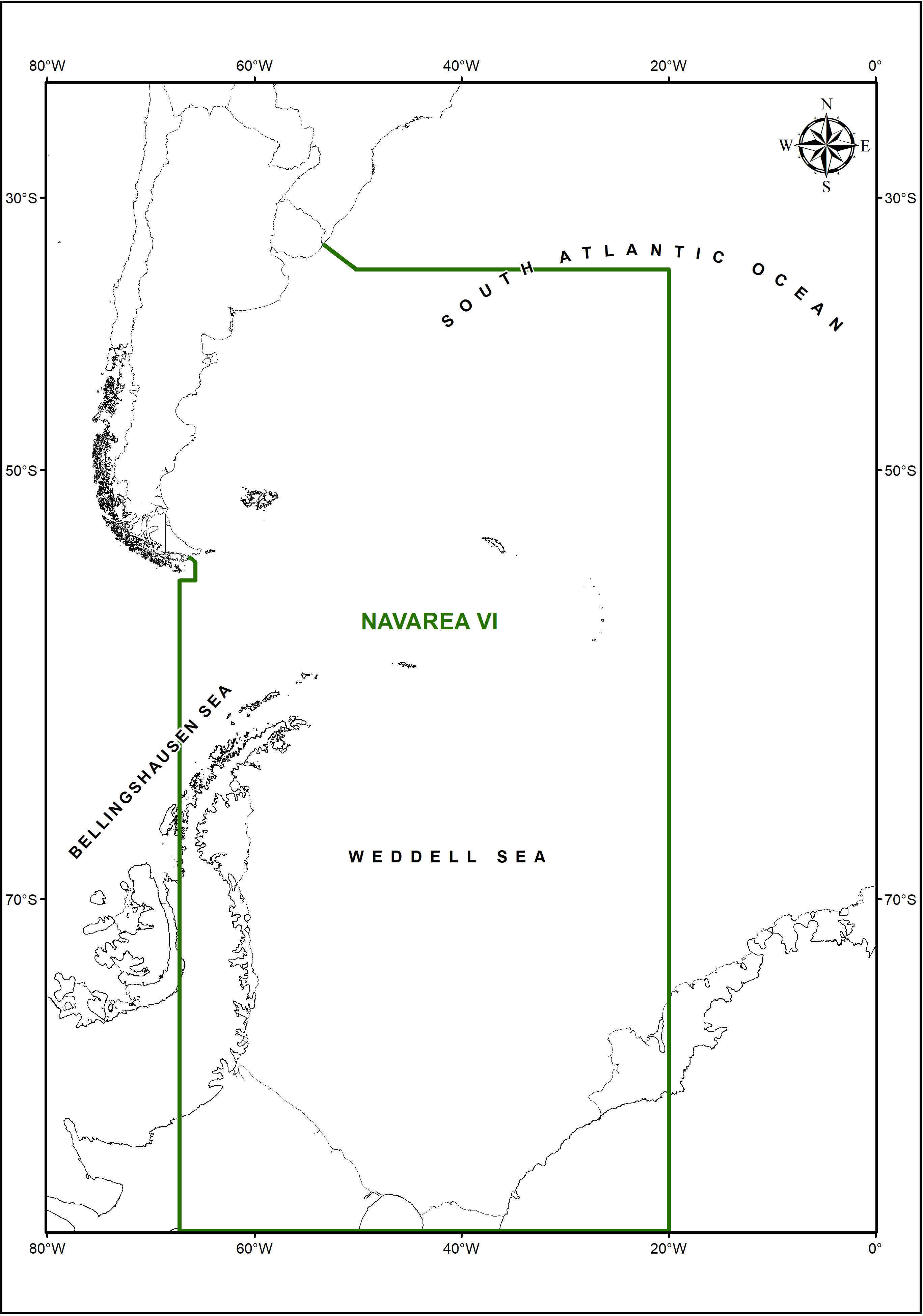
Figure 1 The NAVAREA VI, the Argentine area of responsibility for Safety at Sea information service, directed by the Naval Hydrographic Service.

FIGURE 2

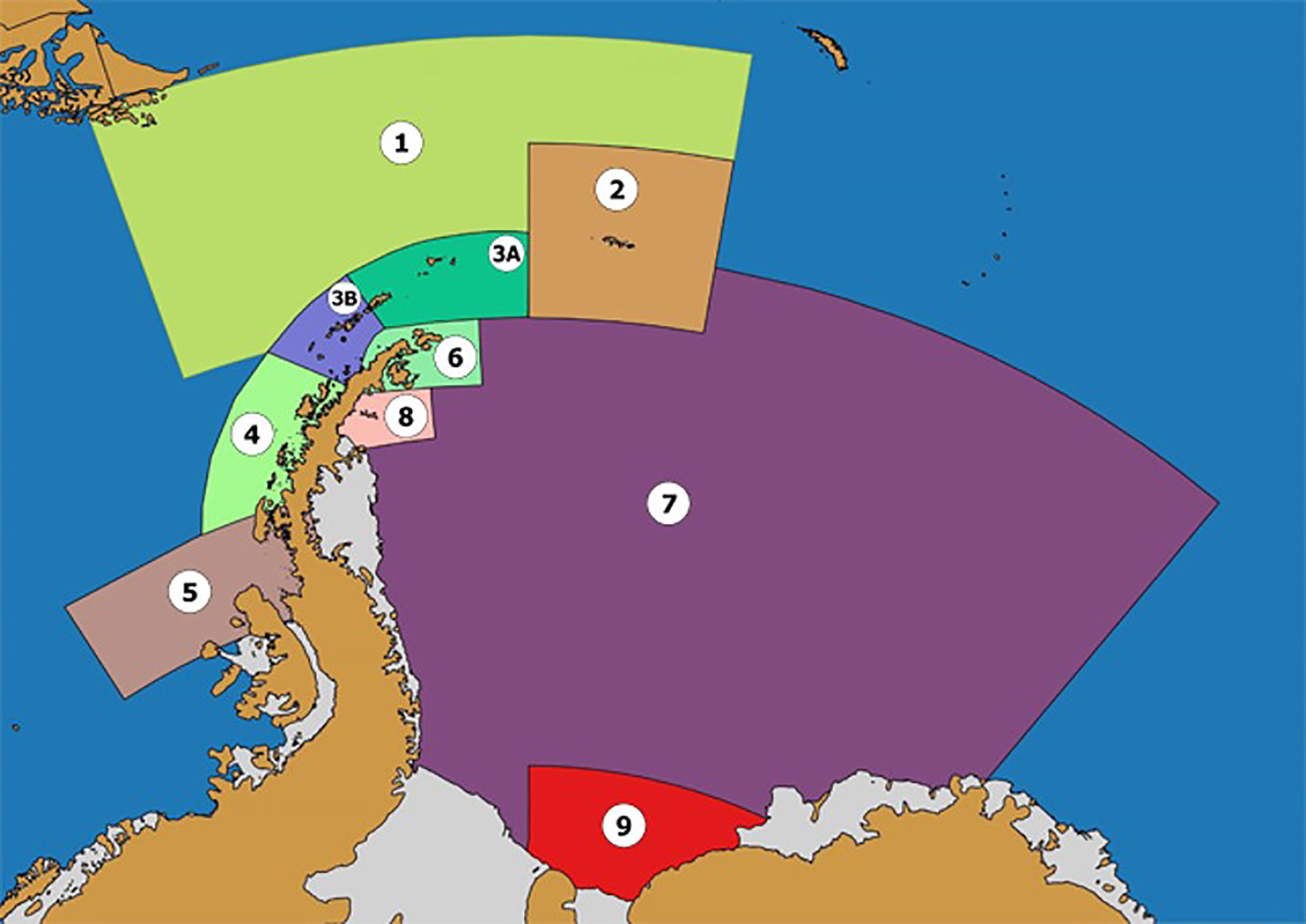
Figure 2 Sub-areas of ice charting production. Zone 1: Drake Passage. Zone 2: South Orkney Islands. Zone 3: Mar de la Flota Straight and South Shetland Islands (with sub-zones 3A and 3B). Zone 4: Channel to Belgrano Island. Zone 5: Bellingshausen Sea and Margarita Bay. Zone 6: Antarctic Strait and Erebus and Terror Gulf. Zone 7: Weddell Sea. Zone 8: Northwest Weddell Sea. Zone 9: South Weddell Sea (Halley station to Berkner Island).

The sub-areas of ice charting production presented in Figure 2 are considered to be high priority areas due to their relevance for research and tourist vessels, and multi-purpose operations that require more detailed sea-ice information.

Information sources

Information sources used as input for the production of ice charts are presented as the following:

Reconnaissance and in situ observations: coastal monitoring, ship-based and aircraft observations.

Observations from Argentine ships and coastal bases in Antarctica are conducted by personnel that undergo training procedures throughout the year, mandated by the SHN, to be approved as ice observers. Observations are collected and archived using the Glaciological Information System (SIGLAC, in Spanish) system, which registers sea ice parameters - such as concentration, stage of development, shape, topography and melting - and the amount of icebergs present. This software includes a quality control component during the observation input phase, that is converted into a numerical coded format for simplification and to unify the interpretation processes by analysts. Once the information is received, in near real-time, it is decoded and applied to second quality control, to be used in the validation of ice charts. All observations are stored in the SHN’s ice database, not currently available for open access.

The advantage to recording observations by a well-trained crew is that it provides a reliable source of information from several places in Antarctica, especially those made from the vicinity of inlets, bays, or coves where vessels need to maneuver for operations. Currently, Argentina supports ice observations from 13 stations, between permanent and temporary ones, distributed throughout the Antarctic Peninsula, Bellingshausen Sea and the east of the Weddell Sea.

Additionally, international merchant vessels and those coming from the Southwestern Atlantic Ocean provide additional information by notifying SHN of the presence of icebergs. Though these observations are not made by trained personnel, they are usually accompanied by photographs and geolocation information that provides ground-truth to corresponding satellite images. This information is extremely valuable to track larger icebergs that are drifting outside Antarctic waters and represent a serious hazard to mariners.

Aircraft observations of sea ice and icebergs are registered during logistic flights. These are primarily used to calibrate and validate satellite imagery and to update general information about the sea ice pack position, concentration and iceberg tracking. Observations from aircraft do not follow the standard format as those from ships or bases, although they are geolocated photographs (Figure 3).

FIGURE 3

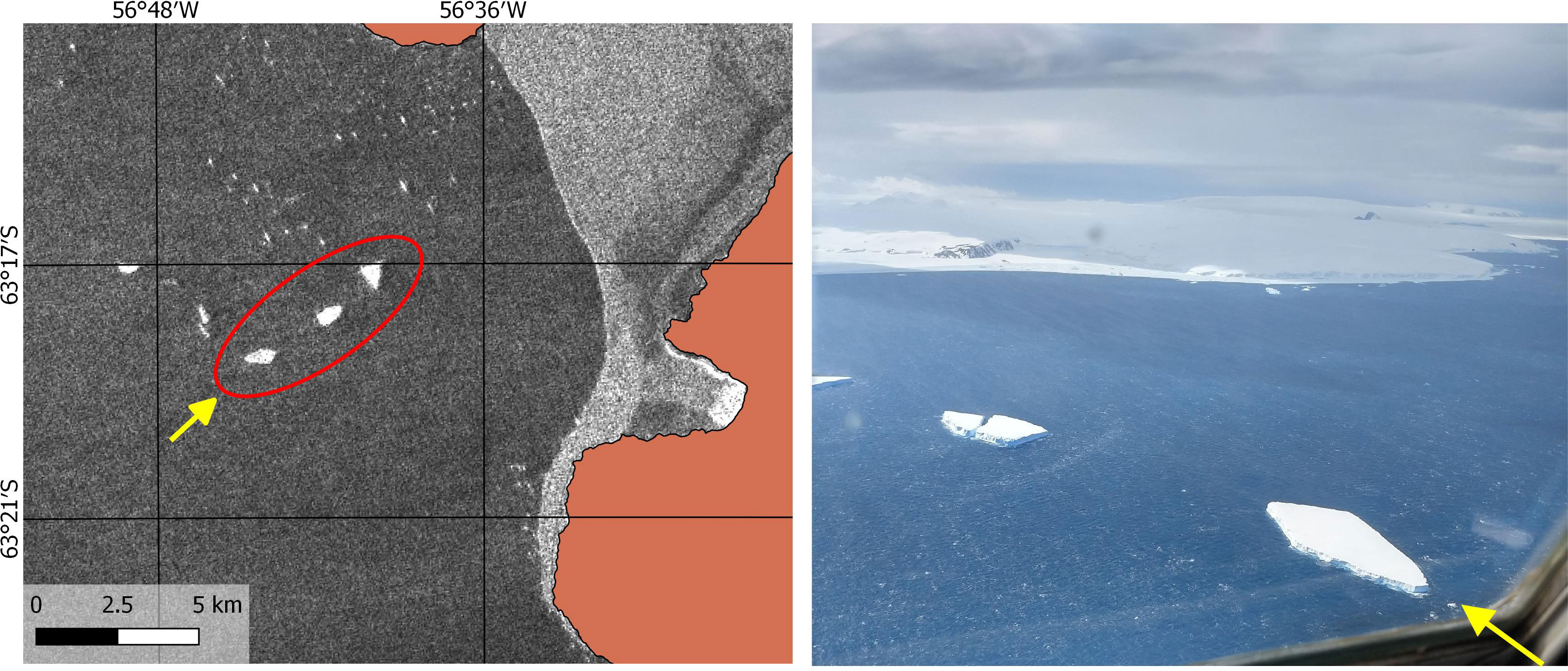
Figure 3 Observation of icebergs during a flight over Joinville Island (right) to validate SAOCOM image (left), from November 19, 2020. The yellow line correspond to the approximate route of the aircraft and the red circle marks the position of the observed icebergs (Satellite image provided by CONAE).

Optical satellite imagery (Visible and Infrared)

The primary sensor used for optical images analyzed at the SHN are the Moderate Resolution Imaging Spectroradiometer (MODIS), operational on the Terra and Aqua satellites, and the Visible Infrared Imaging Radiometer Suite (VIIRS) images from the Suomi National Polar-orbiting Partnership satellite (Suomi NPP). The MODIS and VIIRS imagery present multiple spatial resolutions, depending on the spectral bands. Resolutions corresponding to MODIS are 250 meters and 500 meters, while VIIRS has 375 meters and 750 meters,. Sea ice and icebergs are often identified using corrected reflectance in RGB composites of True and False Color. This optical imagery has the advantage of large spatial coverage with daily revisit for polar regions. However, in this type of image, the ice detection is obstructed by cloud cover or by the lack of solar light during the polar night in the winter season. In fact, high stratiform cloudiness can present spectral signatures similar to ice, which can make it difficult to distinguish, even with RGB combinations. The spectral bands that are frequently used go from the visible to the near-infrared region in the combination 3-6-7 and 7-2-1 for the MODIS Terra sensor, 7-2-1 for the MODIS Aqua sensor, and M11-I2-I1 and M3-I3-M11 for the VIIRS sensor. These combinations make it possible to easily detect ice or snow because of its spectral signature and filter the cloudiness which poses the main challenge when monitoring floating ice.

During low-light conditions, images from Day/Night Band (DNB) of the VIIRS sensor are often used, capturing low light emissions with those reflected by ice being sufficient for detection (Lee et al., 2006). The spatial resolution for this band is 750 meters with daily acquisitions and its combination with other optical images allows to obtain more information regarding the movement of cloud cover, taking advantage of the different schedules of satellite orbits.

Although the spatial resolution of optical satellites is low, as detailed on previous paragraphs, for a detailed analysis of sea ice and small icebergs, it makes it possible to have more regional information during the operational season for critical areas in the ice charts. Additionally, the aforementioned images can be obtained free of charge, provided by the Global Imagery Browse Services (GIBS) as part of the Earth Observing System Data and Information System (EOSDIS) of the National Aeronautics and Space Administration (NASA).

Microwave satellite imagery

Currently, the active microwave sensor Synthetic Aperture Radar (SAR) is the most essential instrument for monitoring floating ice and can be used under any weather and illumination conditions, especially over the polar regions where cloud cover and absence of sunlight in winter make observations difficult with other onboard satellite instruments.

Different frequencies (bands) of the SAR systems are used for glaciology purposes, being mainly the X (8–12.5 GHz, 2.4–3.8 cm), C (4–8 GHz, 3.8–7.5 cm) and L (1–2 GHz, 15–30 cm) bands those with the highest application (Dierking, 2013). Current operational satellites are TerraSAR and COSMO-Skymed in X band, Sentinel-1 and RADARSAT-2 in C band; and ALOS-PALSAR-2 and SAOCOM-1 in L band. SAOCOM-1 consists of two Argentine satellites complementing the SIASGE constellation (Sistema Italo Argentino de Satélites para la Gestión de Emergencias, as in Spanish) with the Italian satellites COSMO-Skymed. SAOCOM-1, launched in 2018, has enabled Argentina to increase the amount of data analyzed for the production of ice charts (Figure 4).

FIGURE 4

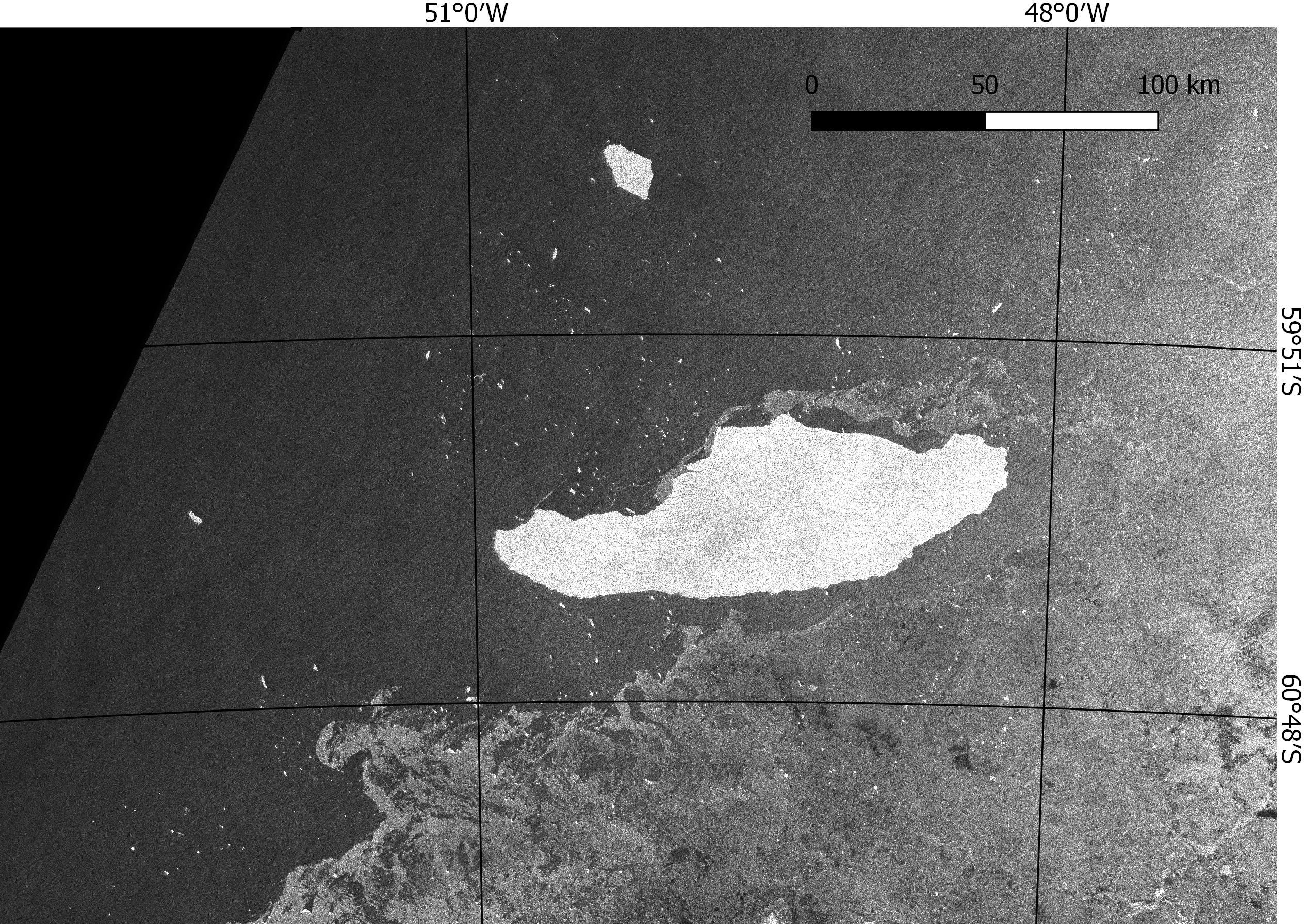
Figure 4 SAOCOM image from May 23 - 2020, showing A68A and A68C icebergs and sea ice in the Weddell Sea (Satellite image provided by CONAE).

SAR images have spatial resolutions that range from 3 to 100 m and wide swath from 20 to 400 km (depending on each satellite instrument and acquisition mode selected)-, allowing a high level of detail over a relatively large area (Dierking, 2013). The spatial resolution and size of the images will depend on the sensor and the acquisition mode. In general, acquisition modes in SAR systems are Spotlight, Stripmap, Scansar and the newer Topsar mode incorporated into Sentinel-1 and SAOCOM-1 satellites (De Zan and Monti Guarnieri, 2006). The Topsar and Scansar modes cover a larger area over Spotlight and Stripmap but yield lower spatial resolutions. Some SAR systems can also obtain polarimetry information for the observed surface using the polarization of received and transmitted signals combining the orientation of the vectorial electric field (Onstott and Shuchman, 2004; Dierking, 2013).

Unlike optical images, SAR images have specific geophysical characters that can affect photo interpretation, thus requiring analysis from specifically trained personnel. It is necessary to understand the scattering mechanisms from the objects of interest in response to the radar signal considering the dielectric properties and the roughness of the observed surface (Onstott and Shuchman, 2004). Characteristics of SAR systems such as the frequency (band) in which the sensor operates, the polarization and the incidence angle determine differences within a scene and must be considered by the ice analyst. Additionally, the coverage of SAR images is limited for regional areas, and the availability of scenes in Antarctic region depends on the frequency of acquisition of each satellite. Some images are usually provided free of charge for predetermined orbits (i.e., Sentinel 1) while others require on-demand and tailored acquisitions, usually at additional cost.

Products derived from passive microwave satellites are used for ice charts to observe sea-ice concentration using the Advanced Microwave Scanning Radiometer (AMSR-2) sensor onboard the GCOM-W satellite (Meier et al., 2018). Even though this data is available year-round, it is mostly used in the absence of illumination during the Southern Hemisphere winter for latitudes south of 60° S when optical images can no longer be used. The reason of this criteria in the use of AMSR-2 data is that the spatial resolution of 12 km is considered too low for a detailed analysis of ice conditions.

Elaboration of the ice charts

Currently, the SHN produces three types of ice charts: sea-ice concentration, ice edge, and iceberg; all three published weekly on the SHN website (www.hidro.gob.ar). Iceberg charts have been published since 2019 on the PolarView portal (www.polarview.aq), yet this is currently in trial mode. QGIS software (www.qgis.org) is used for ice charting production, a reliable, free and open-source solution to the requirements of the SHN. Satellite imagery analysis is performed by trained ice analysts with previous experience in data interpretation of optical and SAR imagery, and a comprehensive knowledge on Antarctic climatology and marine glaciology. The nomenclature and standards used in the generation of the ice charts described in this paper correspond to the publication WMO Sea Ice Nomenclature: Volume I – Terminology and Codes, Volume II – Illustrated Glossary and Volume III – International System of Sea Ice Symbols (WMO No. 259, 2014b). The methodology of ice charting and the description of the final product is explained in the Results section.

Result

Analysis of the information

The first step at the beginning of the charting procedure is to analyze the complete set of data that is available in near-real time. This begins with the ice analyst’s work through visual interpretation of satellite images, combined with observations received from ships and stations in Antarctica. The characteristics to be identified are the extent, the stage of development, the shape and spatial distribution of sea ice. Icebergs presence are also analyzed in terms of their quantity and later tracking. To recognize these variables in the data, well trained analysts must have a good understanding of the object of study and the source of information used.

The object of study, sea ice and icebergs, is directly affected by different environmental variables. Wind and ocean currents determine drift, sea-surface temperature influences formation and melting processes and tidal currents have a local effect on sea-ice concentration in coves, bays and straits. A snow cover modifies the physics of the sea-ice surface and may obscure the stage of development. In order to have complete knowledge of the formation processes of snow cover and sea ice, the analyst needs to understand the climatological and glaciological regimes in the different regions of Antarctica.

Another subject to be covered in the training of ice analysts is the spatial and temporal scale of different satellite sensors and their integration with consistent criteria in the chart products. Additionally, observations from ships and stations are received in a coded format and need a proper training to rapidly understand the information, discriminate the relevant data and integrate them with the satellite imagery in the digitization of ice charts.

Optical images allow for an almost intuitive photo interpretation under cloud-free conditions when respective RGB composites are used. Clouds can obscure the surface and therefore present an obstacle in the identification of sea ice and icebergs, especially when the area of interest is below a dense stratiform cover. RGB composites that include bands from the visible and near-infrared channels can be of great help in distinguishing ice on the ocean from clouds in these situations. For example, the RGB combination of MODIS sensor Band 3-6-7 allows for enhancing the presence of snow and ice in reddish colorations, because these objects are reflective in band 3, corresponding to the visible spectrum, and absorbent in bands 6 and 7, infrared channel (Figure 5). Due to its spectral signature, a cloud cover is typically represented in white in the composite of those three mentioned bands and the open waters appear in dark colors. Therefore, it is possible to find a cloud-free location of sea ice and icebergs despite cloudiness. However, occasionally small ice crystals of Cirrus clouds appear in reddish orange with the aforementioned RGB composite, which means a detailed analysis is necessary to not confuse the ice on the ocean surface with that in the clouds.

FIGURE 5

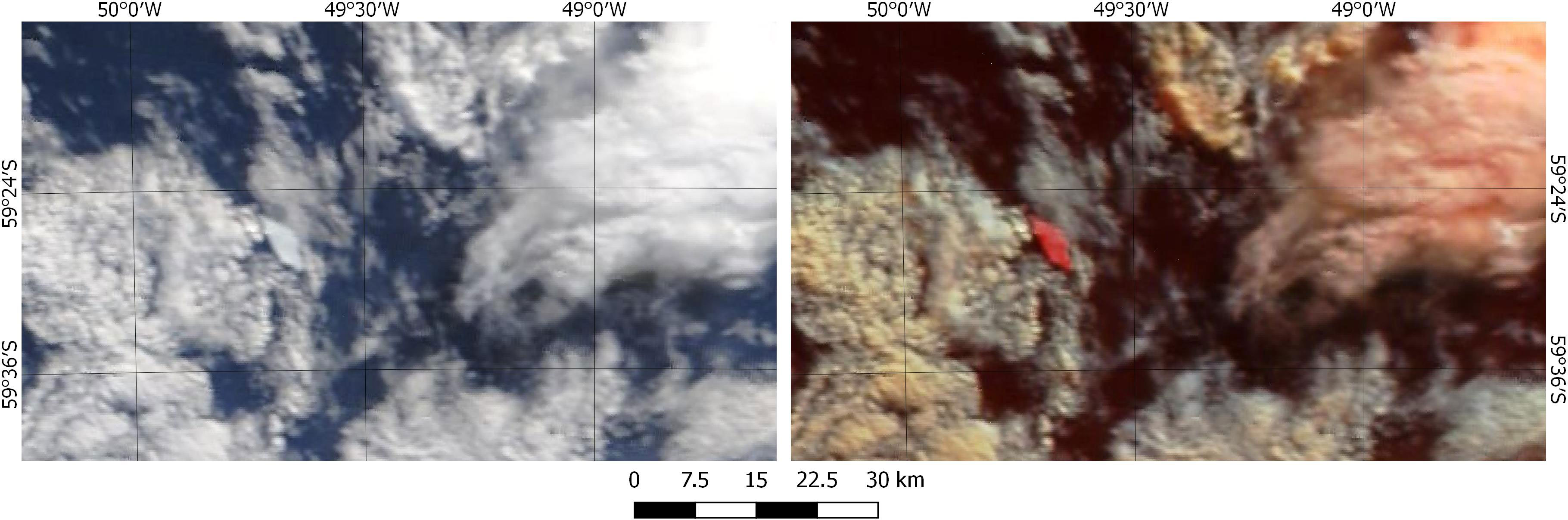
Figure 5 Iceberg and cloudiness in MODIS Terra image from April 5 - 2020, in true color (left) and RGB 3-6-7 composite (right).

On the other hand, SAR systems, by employing the transmission of electromagnetic pulses in the microwave range to receive the energy backscattered from the surface, not only require trained personnel to understand the response of the objects to be analyzed, but also constant training and familiarization for the correct data.

Ice analysts can recognize the different types of ice in the SAR images by interpreting the intensity of the response, the texture and the shape of the different objects. The observed characteristics of those elements are integrated with the knowledge of the dielectric properties and the roughness of the surface of each class of ice. Also, radar frequency used is mainly considered, which determines the penetration of the signal into the surface and the angle of incidence of each image.

In large-scale SAR imagery (around 250 km swath coverage), such as ScanSAR and TopSAR, very small or large incidence angles can present difficulties in detecting ice, and in the worst-case scenario, the presence of ice is note noticeable in the SAR scene. Example of this can be seen in Figure 6, where sea-ice belt and strips are hardly detected. An ice analyst familiar with this type of image can determine the presence of the ice even when it is not as clearly defined by the sensor.

FIGURE 6

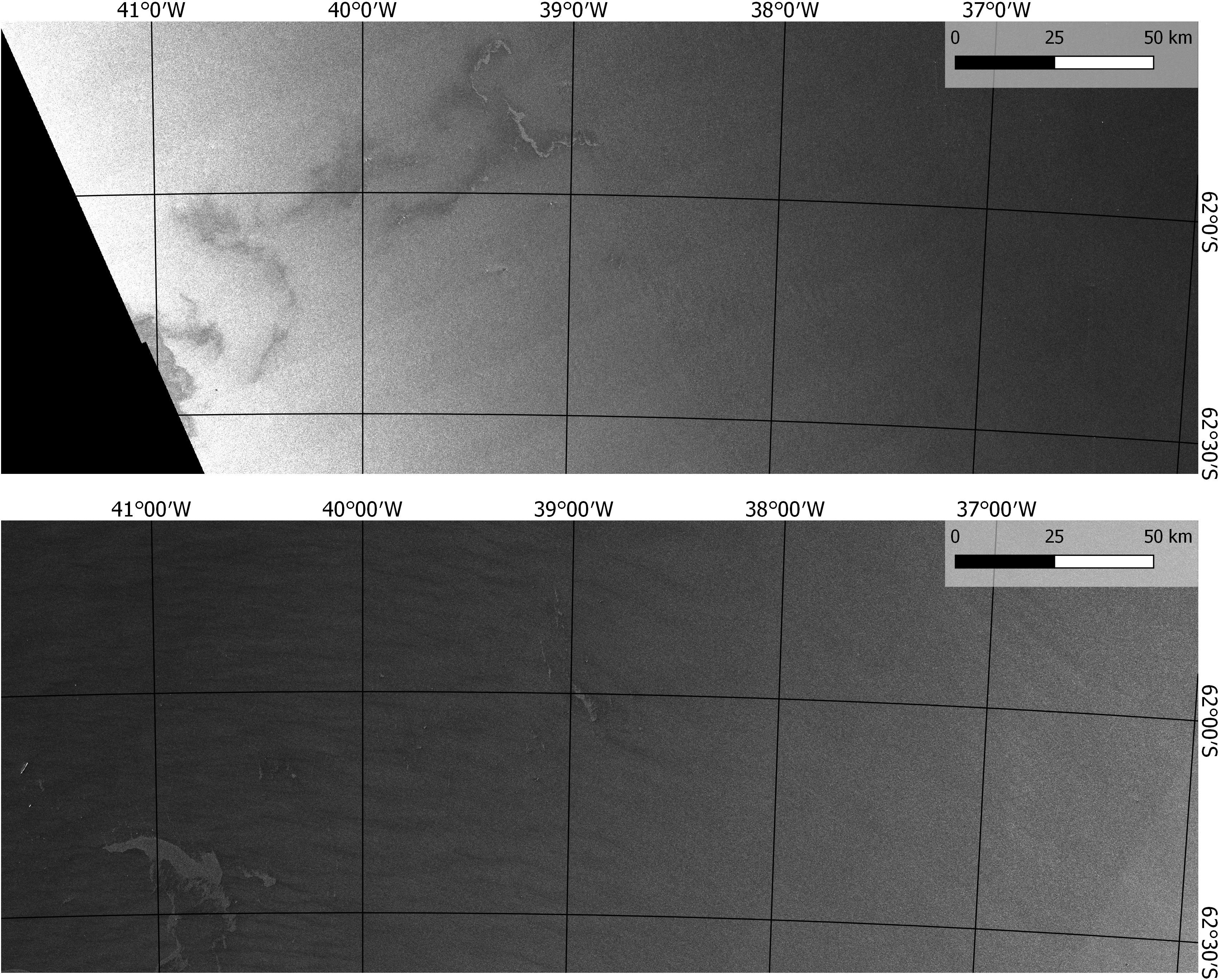
Figure 6 Belts and strips in Sentinel-1 image from April 4 (top) and April 5 (bottom), 2020 in the Weddell Sea. Near and far range of each image, respectively. Copernicus Sentinel data 2020, processed by ESA.

Information sources are not always updated at the time of the analysis, and some observations or satellite images may correspond to the previous 48 hours. Analyzes are carried out considering the variations that sea ice has suffered and the drift of icebergs in that period. Meteorological, oceanographic and even statistical climatological data must be incorporated in the charting process.

Sea-ice concentration charts

For the preparation of the sea-ice concentration charts, generally known as ‘ice charts’, homogeneous areas in the sea-ice concentration are identified. The World Meteorological Organization Nomenclature defines concentration as the fraction of the sea surface covered by ice, expressed in tenths (WMO No. 259, 2014b). The analysis of the area in which the different concentrations are divided will depend on the spatial scale used in the digitalization, the source of the information and the spatial resolution. The concentration is classified with categories ranging from 0/10 (open water) to 10/10 (the entire surface covered) of sea ice and polygons are generated in vector format files, following the definitions and standard colors of the Color Code Ice Chart Standard (WMO No. 1215, 2014a) (Figure 7).

FIGURE 7

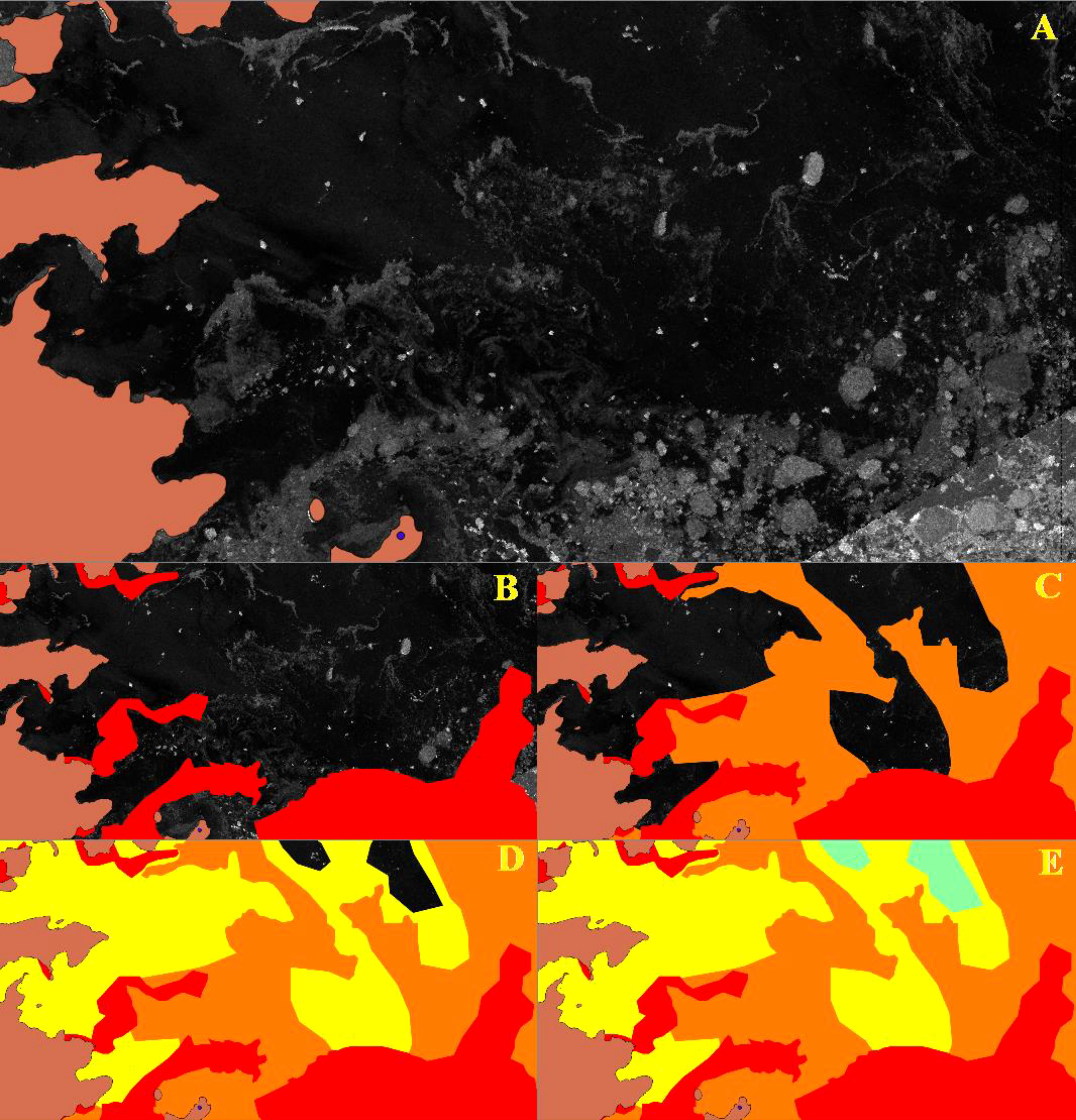
Figure 7 Digitization of sea-ice concentration polygons in the Erebus and Terror Gulf. (A) Sentinel-1 image from March 30, 2020. (B) Polygons with concentration 9-10/10, (C) adding polygons with concentration 7-8/10, (D) adding polygons with concentration 4-6/10 and (E) adding polygons with concentration 1-3/10. SHN 2020, contains modified Copernicus Sentinel data 2020, processed by ESA. Color code is available in Figure 8.

The predominant form and stage of development of sea ice are coded using ice-chart symbology combined in the so-called Egg Code. This code is represented by an oval subdivided into four horizontal sections. The first one at the top indicates the total concentration of the sea ice in tenths. In the second section, partial concentrations are indicated, while in the third and fourth the stages of development and the forms, respectively, of each of the partial concentrations are reported. In those polygons where the presence of icebergs is detected, a black triangle is included on the side of the oval.

Figure 8 shows the ice chart for April 1 - 2020, corresponding to the Antarctic Strait and the Erebus and Terror Gulf. Digitized ice concentrations for the area can be seen with Egg Codes for each polygon. In this particular situation, the polygon indicated with an A has a sea-ice concentration of 1-3/10 with egg code reporting partial concentrations of 1/10 for the stages of development ‘7. 6 3’, corresponding to old, first year and young ice. The form in the fourth section is informed with (~ 10) symbology where strips and patches can be found in that concentration area. The black triangle indicates the presence of icebergs.

FIGURE 8

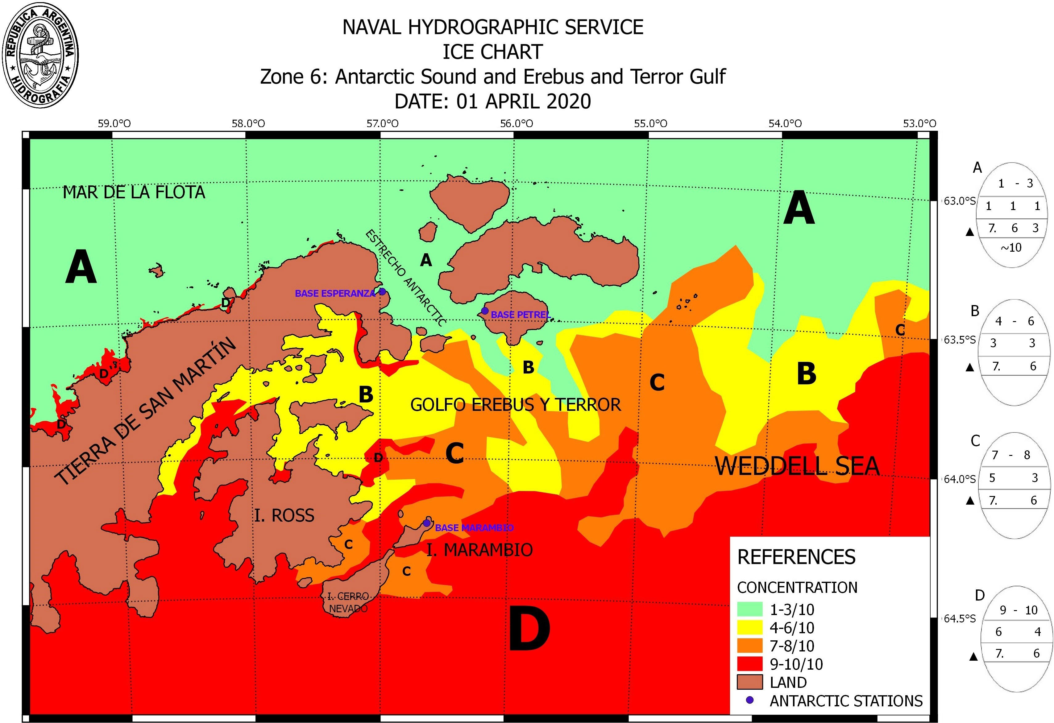
Figure 8 Ice chart dated April 1, 2020. Zone 6: Antarctic Strait and the Erebus and Terror Gulf.

These ice charts provide detailed information on sea ice, but only indicate the presence or absence of icebergs in the egg code. Nine sea-ice concentration charts are generated weekly and in the case of significant changes due to environmental conditions, the frequency of updates increases; especially in the highly visited area of the Antarctic Peninsula.

Ice edge charts

The Ice Edge chart is made to establish the general limits of the ice edge and the marginal ice zone, allowing mariners to know which areas of navigable waters are free of sea ice. It is useful for ships that do not have intent to navigate in the Antarctic region but also need to make their way through the Drake Passage, which connects the South Atlantic Ocean with the South Pacific Ocean, or ships that sail north of the Antarctic Peninsula during spring and winter when the ice field extends the most to the northern waters.

As it was mentioned before, using the different satellite images, the presence of sea ice is observed and delimited with the digitization of polygons in vector format. In the analysis, the ice edge, compact and diffuse, and the marginal zone are distinguished. According to standardized nomenclature, the ice edge is the demarcation between the sea ice of any kind and the open sea. Operationally, this definition is considered for the delimitation of the ice edge and also the criterion is taken to consider those ice concentrations between 4-10/10. The marginal ice zone is defined as the region covered with ice that is affected by waves that penetrate the open areas of sea ice. For the digitization of the charts, concentration polygons of 1-3/10 are considered. Red polygons indicate the ice edge and yellow ones, the marginal ice zone (Figure 9).

FIGURE 9

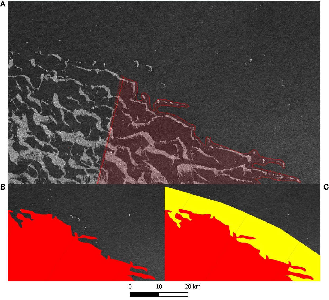
Figure 9 Generation of the ice edge chart using satellite images. (A) digitization of the Sentinel-1 image on March 31, 2020 in the Weddell Sea. (B) polygon of the ice edge (red) and (C) the addition of the marginal ice zone (yellow). SHN 2020, contains modified Copernicus Sentinel data 2020, processed by ESA. Color code is available in Figure 8.

In sectors where a diffuse ice edge is seen, broken sea-ice strips and belts may not be fully incorporated into the ice edge and belong in part to the marginal ice zone (Figure 9). The analyst should prioritize the areas to be included in these polygons to clearly transmit the information about the sea-ice condition. The user should keep these considerations in mind, in case the only available information is the ice edge charts.

Two ice edge charts are generated weekly. Figure 10 presents a completed ice chart for May 26, 2020. It should be noted that this chart only refers to sea ice and does not indicate the presence or absence of icebergs, mariners should consult the iceberg chart so as not to incur risks during navigation nearby the sea-ice edge.

FIGURE 10

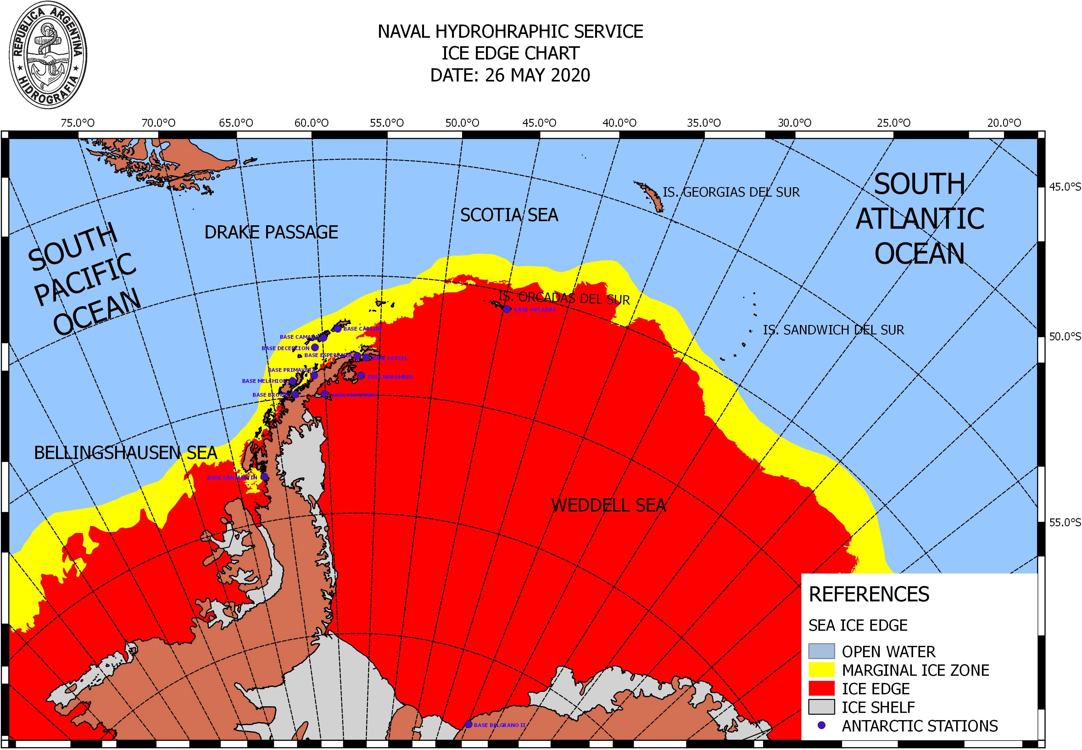
Figure 10 Ice edge chart from May 26, 2020. Ice edge is defined as the limit of sea-ice concentration above 4/10.

The same information is summarized in several waypoints and transmitted through SafetyNET and NAVTEX systems for duplication of communications to ensure that the location of sea-ice edge is acquired by all vessels in the NAVAREA VI and vicinities.

Iceberg charts

The Iceberg Chart identifies the position of icebergs in open waters or next to the sea-ice edge. Icebergs with dimensions greater than 10 nautical miles, named by the US NIC using a letter from the region of Antarctica where it calved, and a cumulative number, are indicated in the iceberg chart with colored dots. Icebergs with smaller dimension between10 and 2 nautical miles are marked with blue colored dots, differentiating them from internationally renowned (Figure 11).

FIGURE 11

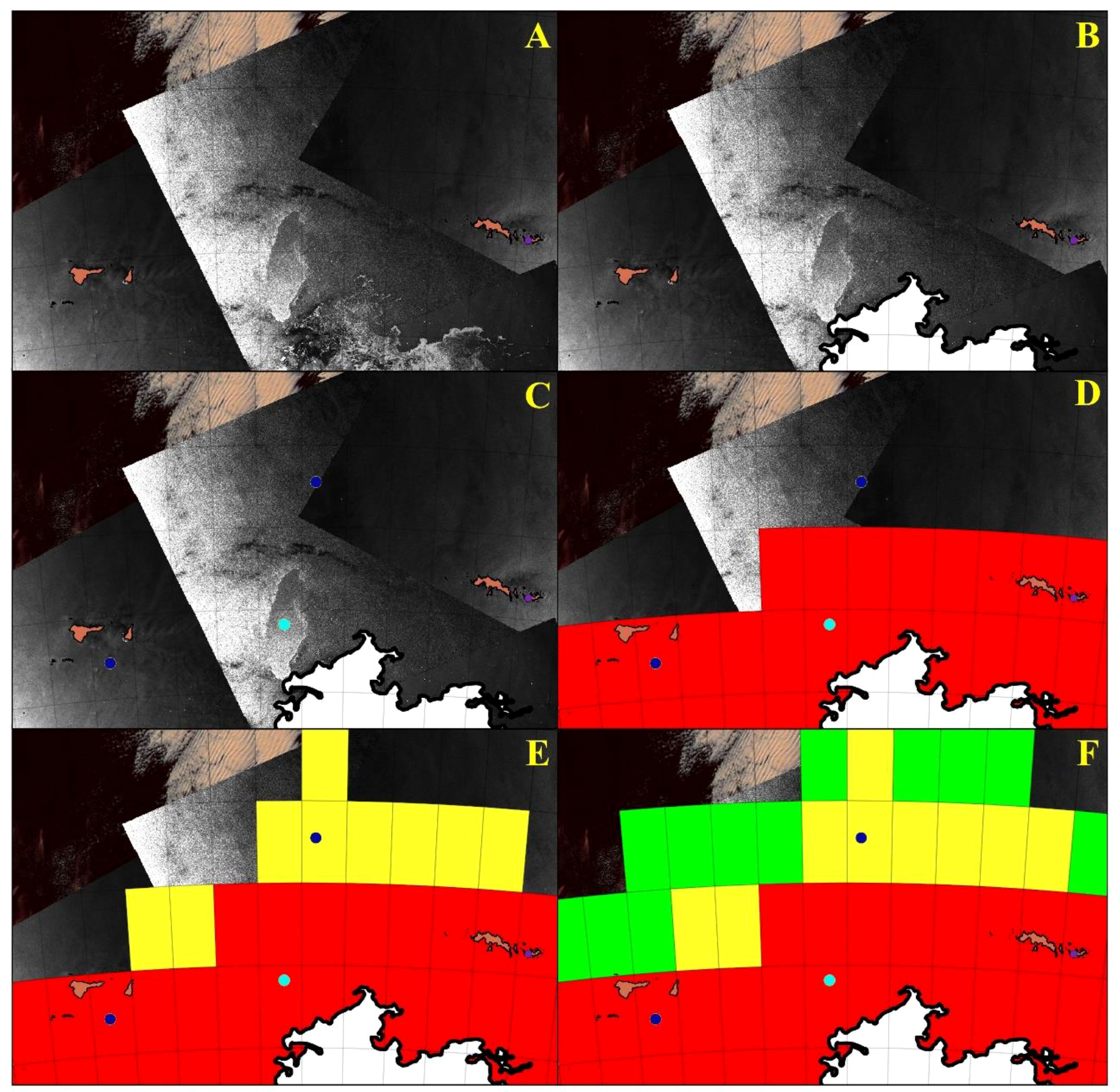
Figure 11 (A) Sentinel-1 image of April 2, 5 and 6 2020 and VIIRS Suomi NPP of March 28, 2020 in the South Orkney Islands sector. (B) Compact ice edge delimited in white. (C) A68A iceberg positioned with a cyan dot and smaller iceberg in blue dot. Digitized cells as a risk area for (D) ‘many icebergs’ (E) ‘few icebergs’ and (F) ‘isolated icebergs’. SHN 2020, contains modified Copernicus Sentinel data 2020, processed by ESA.

Icebergs with smaller dimensions than 2 MN are include in areas indicating the risk of finding icebergs in a certain amount, named as ‘Iceberg Risk Areas’. These areas are distinguished by the number of icebergs recorded in a grid cell of 1-degree latitude by 1-degree longitude. If the grid contains only 1 iceberg, it is classified as ‘isolated icebergs’ (green cells), between 2 and 6 icebergs it corresponds to ‘few icebergs’ (yellow cells), and for an amount of 7 icebergs or higher, it is called ‘many icebergs’ (red cells), as shown in Figure 11. Working with risk areas definitions saves operating time for the analysts by providing a large amount of detailed information for safety of navigation in waters infested by numerous icebergs.

Special focus is dedicated to those icebergs drifting in the Drake Passage or even further north in the Argentine Sea. The drift to the north and beyond the limits of the Antarctic Circumpolar Current is the consequence of the effect of the Malvinas Current that deflects to the north, towards warmer latitudes, representing a real hazard in regions of the South Atlantic Ocean where these floating objects are not expected by Officers on Watch at the bridge of a ship. Furthermore, warmer water generates a gradual decrease in the size of the iceberg due to melting and iceberg detection gets more difficult due to the spatial resolution of the available satellite data. In this situation, reports received by the vessels are extremely valuable information for the iceberg chart provided.

Figure 12 shows the iceberg chart from April 6, 2020. The compact ice edge is represented by the black line and white region, establishing that the risk areas analyzed are in open waters where icebergs constitute a bigger risk for navigation. Icebergs within the ice field are not represented on these specific charts.

FIGURE 12

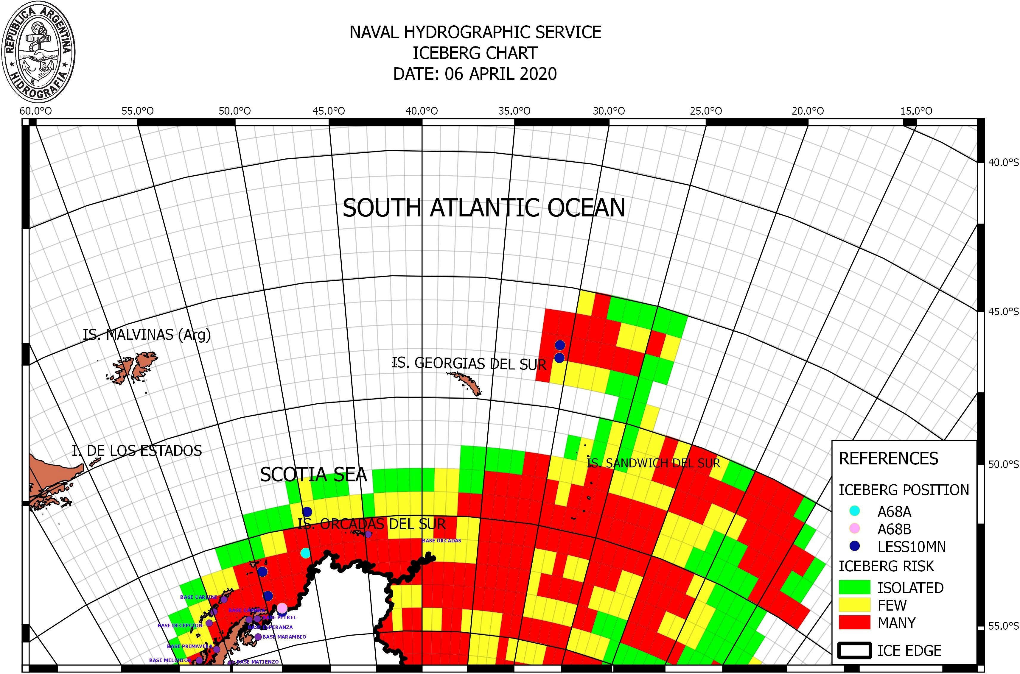
Figure 12 Iceberg chart from April 6, 2020. Grids are sized 1° x 1°. Isolated: only 1 iceberg, Few: from 2 to 6 icebergs and Many: more than 7 icebergs.

As it was mentioned before, the iceberg chart is also uploaded on the PolarView(Figure 13), where it can also be overlaid with other shapes of information from different Ice Services around the world.

FIGURE 13

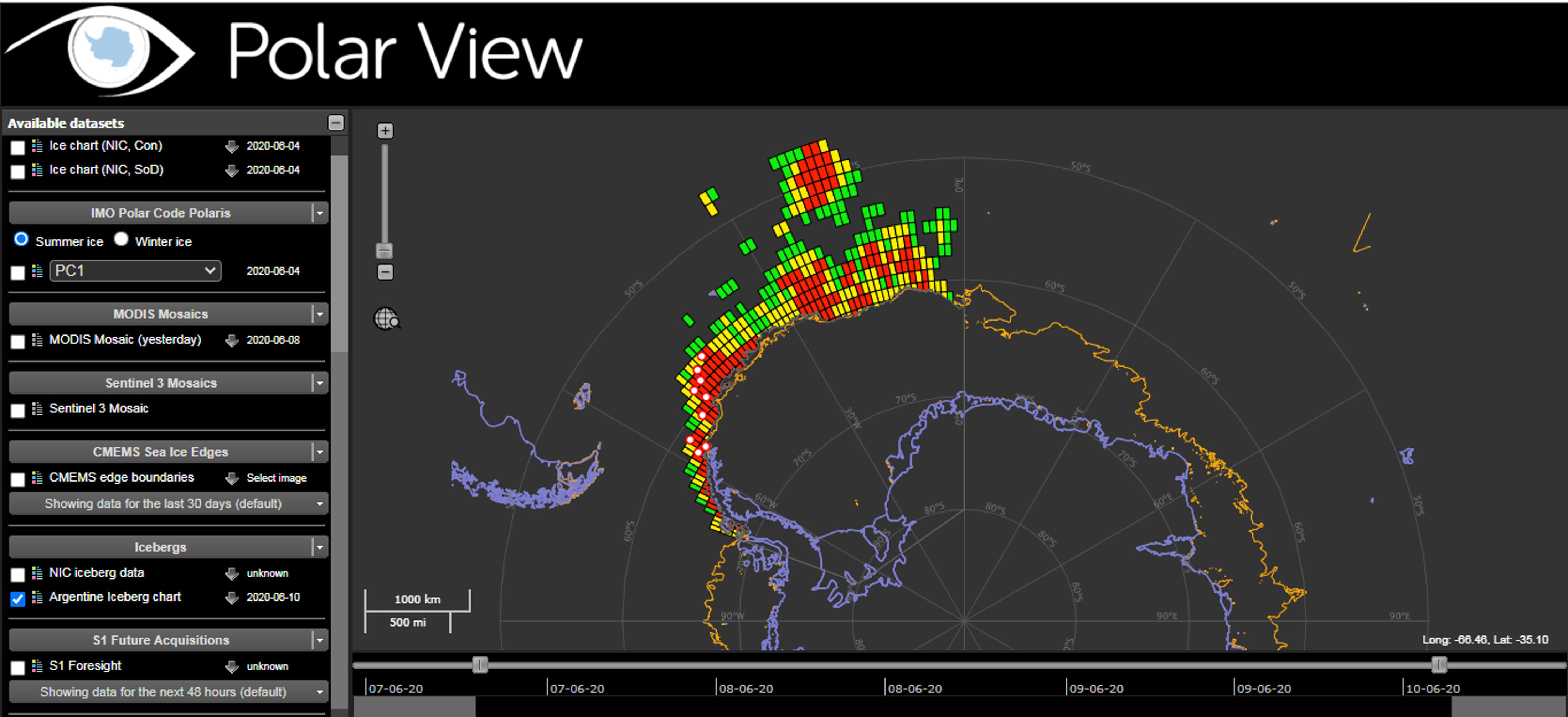
Figure 13 Argentine Iceberg Chart displayed on Polarview’s website.

As for the ice edge, iceberg positions are also included in the SafetyNET and NAVTEX messages to mariners. Information on the position of all known icebergs is transmitted, with daily updates when satellite imagery is available, and areas with the presence of several icebergs by using the position of polygons vertices.

Discussion

The activities carried out on the Antarctic continent require a great logistical effort by all countries that have permanent or temporary stations, being executed mainly by marine transport. Although activities in polar waters of the Antarctic region are minimal compared to the Arctic Ocean, with well-defined trade routes and throughout the entire year, tourist activity and fishing in border regions of Antarctica increase annually. For that reason, it is imperative for countries closer to Antarctica, like Argentina, to provide reliable and accurate support information on the safety of navigation to all ships sailing this remote part of the globe. Even more, if we consider that if an incident occurs in polar or subpolar waters of the Southern Hemisphere, aid would be delayed for several days because of the long distances that exist between Antarctica and the Search and Rescue (SaR) Centers. It is important to inform that iceberg impacts are not the only hazard but also the presence of multi-year sea ice or the increase of pressure in the surrounding sea-ice field.

During the austral summer season, from November to April, the Argentine and Chilean Navy share SaR activities in the Antarctic Peninsula, ensuring the permanent presence of a rescue ship in the area with the highest marine traffic. However, for the rest of the year the aid could take weeks by ship to reach a remote area of ​​Antarctica, with consequent implications of risking human lives or possible ecological disasters. Therefore, to ensure navigation in isolated and potentially dangerous areas subject to rapid variations due to the effect of meteorology and ocean currents, updated ice charts are necessary, which must be constantly improved with the development of new technological tools.

The mission of the Argentine Naval Hydrographic Service (SHN) as a public service is to provide information for safety of navigation in NAVAREA VI. One of these tasks is the provision of the best products and services for ice charting in the Antarctic and South Atlantic Ocean. Although this activity has been carried out uninterruptedly since the 1970s with the use of satellite products, since 2015 ice charts have been produced weekly, with a significant improvement in quality and precision according to the advancement of knowledge and technological tools.

The ice edge charts provide users with regional information on the extent and concentration of sea ice in the Weddell Sea and Bellingshausen Sea. When it is required to know in more detail the glaciological condition, the sea-ice concentration charts in the different areas can be consulted, which also present information on the stage of development and the forms of sea ice. The iceberg chart provides detailed information on icebergs all over the NAVAREA VI, with updated positions and risk areas giving information on their distribution and quantity.

In addition, the systematic and continuous production and storage of ice charts can provide a valuable source of information, validated and quantifiable, to map the detection of changes in the state and condition of both sea ice and icebergs. This information will be of particular interest to cryosphere researchers who are linking changes in sea-ice conditions and extent to climate models.

During the ice charting process, the training and experience of those who perform the analysis is essential. It is fundamental for the ice analysts to be familiar with the region of focus, with an emphasis on understanding the prevailing synoptic environmental variables - such as atmospheric, currents and tides - and climatological - such as glaciological regimes in the formation or deterioration of the ice. Analysts must also be aware of the particularities of each information source to avoid making erroneous interpretations that could constitute a potential hazard to maritime navigation. Different characteristics of the ice (i.e., roughness, thickness or snow cover) may not be detected as easily as expected when the identification through the different types of satellite imagery must be done during operational times, knowing that dozens of vessels will depend on this information.

It should be noted that the manual drawing of ice charts has operator-dependent subjectivities. Partington et al. (2003) highlight that ice analysts have different skill levels according to their fieldwork experiences and knowledge on the specifics of ice. Alternatives to manually generated ice charts are being studied by automating the processes for the detection, classification and estimation of ice concentration (Moen et al., 2013). However, there is currently no conclusive evidence that the tasks of ice analysts can be replaced by automatic processes for operational activities.

As mentioned before, ice analysts have a major responsibility in the ice charting process. SHN’s ice analysts have a rotation of about 5 years, allowing proper training with a high degree of experience in the manual elaboration of ice charts. Transferring experiences to new analysts is also an important concept in the personnel training. Generally, it is intended to incorporate one crew member per year with an increase from 2 to 7 expert analysts since 2015. Systematic errors can be reduced with a consolidated training program and continuous provision of personnel and the adjusted rotation in the assignment of tasks within the Ice Service responsibilities.

An advantage in the training of ice analysts from the SHN is the possibility of sailing in Antarctic waters on board Argentine Navy Ships – an icebreaker, polar supplies or research vessels - making it possible to personally experience navigation within sea ice or near icebergs of different sizes. In this sense, they become aware of the implications of providing the most accurate and updated ice information for nautical safety and the difficulties that mariners experience in the interpretation of ice charts.

Analog to the results obtained by Dedrick et al. (2001), the different ice charts that Argentina produces for Antarctica and NAVAREA VI have increased their quality and reliability remarkably from the following factors:

1. The increase in the availability of SAR imagery, starting with a higher acquisition frequency of Sentinel-1 and since 2018 with the Argentine SAOCOM satellite that represents a significant improvement in working capacity.

2. The ability to handle and process an increasing volume of information and to improve the quality controls of observations made by ships and stations.

3. The possibility of using the Night Vision mode of the SNPP satellite, allowed the improvement in the elaboration of ice charts during the austral polar night.

4. The increase in the number of personnel dedicated exclusively to the task of ice analysts.

5. The collaborative work between the different Ice Services and related organizations around the world, based on the links established through the incorporation to the International Ice Charting Working Group.

We conclude that the regular training of ice analysts in the correct use of information sources is essential and one of the key objectives of the SHN. This enables SHN to issue best quality products by integrating all near real-time information available and serve the public by providing relevant information for safety of navigation to mariners in Antarctic and South Atlantic waters. This paper is intended to make the information published in the ice charts visible for all end-users in order to enable a more in-depth interpretation.

Author contributions

Equal contribution: AS and CS. Last authorship: LS. All authors contributed to the article and approved the submitted version.

Acknowledgments

The authors acknowledge the support of WMO for the publication of this paper, as a contribution to better supporting sea ice services in the Southern Ocean. The authors acknowledge the use of imagery from NASA’s Worldview application (https://worldview.earthdata.nasa.gov), part of NASA’s Earth Observing System Data and Information System (EOSDIS).

Conflict of interest

The authors declare that the research was conducted in the absence of any commercial or financial relationships that could be construed as a potential conflict of interest.

Publisher’s note

All claims expressed in this article are solely those of the authors and do not necessarily represent those of their affiliated organizations, or those of the publisher, the editors and the reviewers. Any product that may be evaluated in this article, or claim that may be made by its manufacturer, is not guaranteed or endorsed by the publisher.

References

Arias Duarte L. P., Santacruz Delgado A. M., Posada E. (2010). Programa satelital colombiano de observación de la tierra: una estrategia de innovación y desarrollo tecnológico para Colombia. Rev. del Instituto Geográfico Agustín Codazzi. 44, 13–29.

Google Scholar

Dedrick K. R., Partington K., Van Woert M., Bertoia C. A., Benner D. (2001). U.S. National/Naval ice center digital Sea ice data and climatology. Can. J. Remote Sens. 27:5, 457–475. doi: 10.1080/07038992.2001.10854887

CrossRef Full Text | Google Scholar

De Zan F., Monti Guarnieri A. (2006). TOPSAR: Observation by Progressive Scans. IEEE Trans. Geosci. Remote Sens. 44 (9), 2352–2360. doi: 10.1109/TGRS.2006.873853

CrossRef Full Text | Google Scholar

Dierking W. (2013). Sea Ice monitoring by synthetic aperture radar. Oceanography 26, 100–111. doi: 10.5670/oceanog.2013.33

CrossRef Full Text | Google Scholar

Divine D. V., Dick C. (2006). Historical variability of sea ice edge position in the Nordic seas. J. Geophys. Res. 111 (C01001). doi: 10.1029/2004JC002851

PubMed Abstract | CrossRef Full Text | Google Scholar

Divine D. V., Pedersen C. A., Karlsen T. I., Faste Aas H., Granskog M. A., Hudson S. R., et al. (2016). Photogrammetric retrieval and analysis of small scale sea ice topography during summer melt. Cold Regions Sci. Technol. 129, 77–84. doi: 10.1016/j.coldregions.2016.06.006

CrossRef Full Text | Google Scholar

Hall R. J., Hughes N., Wadhams P. (2002). A systematic method of obtaining ice concentration measurements from ship-based observations. Cold Regions Sci. Technol. 34 (2), 97–102. doi: 10.1016/S0165-232X(01)00057-X

CrossRef Full Text | Google Scholar

International Association of Antarctica Tour Operators (2020). Available at: https://iaato.org/.

Google Scholar

Knol M., Arbo P., Duske P., Gerland S., Lamers M., Pavlova O., et al. (2018). Making the Arctic predictable: the changing information infrastructure of Arctic weather and sea ice services. Polar Geogr. 41:4, 279–293. doi: 10.1080/1088937X.2018.1522382

CrossRef Full Text | Google Scholar

Kukla G., Robinson D. (1980). Annual cycle of surface albedo. Mon. Wea. Rev. 108, 56–68. doi: 10.1175/1520-0493

CrossRef Full Text | Google Scholar

Lavergne T., Sørensen A. M., Kern S., Tonboe R., Notz D., Aaboe S., et al. (2019). Version 2 of the EUMETSAT OSI SAF and ESA CCI sea-ice concentration climate data records. Cryosphere 13, 49–78. doi: 10.5194/tc-13-49-2019

CrossRef Full Text | Google Scholar

Lee T., Miller S., Turk F., Schueler C., Julian R., Deyo S., et al. (2006). The NPOESS VIIRS Day/Night visible sensor. Bull. Amer. Meteor. Soc 87, 191–199. doi: 10.1175/BAMS-87-2-19

CrossRef Full Text | Google Scholar

Li T., Zhang B., Cheng X., Westoby M. J., Li Z., Ma C., et al. (2019). Resolving fine-scale surface features on polar Sea ice: A first assessment of UAS photogrammetry without ground control. Remote Sensing 11 (7), 784. doi: 10.3390/rs11070784

CrossRef Full Text | Google Scholar

Mahoney R. A., Barry R. G., Smolyanitsky V., Fetterer F. (2008). Observed sea ice extent in the Russian arcti-2006. J. Geophys. Res. Atmos. 113 (C11). doi: 10.1029/2008JC004830

PubMed Abstract | CrossRef Full Text | Google Scholar

Meier W. N., Markus T., Comiso J. C. (2018). AMSR-E/AMSR2 unified L3 daily 12.5 km brightness temperatures, Sea ice concentration, motion & snow depth polar grids, version 1 (Boulder, Colorado USA: NASA National Snow and Ice Data Center Distributed Active Archive Center). doi: 10.5067/RA1MIJOYPK3P

CrossRef Full Text | Google Scholar

Moen M.-A. N., Doulgeris A. P., Anfinsen S. N., Renner A. H. H., Hughes N., Gerland S., et al. (2013). Comparison of feature based segmentation of full polarimetric SAR satellite sea ice images with manually drawn ice charts. Cryosphere 7, 1693–1705. doi: 10.5194/tc-7-1693-2013

CrossRef Full Text | Google Scholar

Onstott R., Shuchman R. (2004). “Chapter 3: Measurements of Sea ice,” in Synthetic aperture radar marine user's manual. Eds. Apel J. R., Jackson C. R. (Washington, DC. USA: National Oceanic and Atmospheric Administration).

Google Scholar

Partington K., Flynn T., Lamb D., Bertoia C., Dedrick K. (2003). Late twentieth century northern hemisphere sea-ice record from U.S. national ice center ice charts. J. Geophys. Res. 108 (C11), 3343. doi: 10.1029/2002JC001623

CrossRef Full Text | Google Scholar

Pope A., Wagner P., Johnson R., Shutler J., Baeseman J., Newman L. (2017). Community review of southern ocean satellite data needs. Antarctic Sci. 29 (2), 97–138. doi: 10.1017/S0954102016000390

CrossRef Full Text | Google Scholar

Venegas S. A., Drinkwater M. R. (2001). Sea Ice, atmosphere and upper ocean variability in the weddell Sea, Antarctica. J. Geophys. Res. 106 (C8), 16747–16765. doi: 10.1029/2000JC000594

CrossRef Full Text | Google Scholar

Walsh J. E., Fetterer F., Scott Stewart J., Chapman W. L. (2017). A database for depicting Arctic sea ice variations back to 1850. Geogr. Rev. 107, 89–107. doi: 10.1111/j.1931-0846.2016.12195.x

CrossRef Full Text | Google Scholar

Weissling B., Ackley S., Wagner P., Xie H. (2009). EISCAM — digital image acquisition and processing for sea ice parameters from ships. Cold Regions Sci. Technol. 57, 49–60. doi: 10.1016/j.coldregions.2009.01.001

CrossRef Full Text | Google Scholar

World Meteorological Organization (2014a) Chart Colour Code Standard (WMO No. 1215). Available at: https://library.wmo.int/index.php?lvl=notice_display&id=11296#.YppAa3bMI2w.

Google Scholar

World Meteorological Organization (2014b) Sea Ice Nomenclature (WMO No. 259, Volume I – Terminology and Codes, Volume II – Illustrated Glossary and Volume III – International System of Sea-Ice Symbols). Available at: https://library.wmo.int/index.php?lvl=notice_display&id=6772#.YpoywXbMI2w.

Google Scholar

World Meteorological Organization (2021) Sea-ice Information and Services (WMO-No.574). Available at: https://library.wmo.int/index.php?lvl=notice_display&id=7542#.YpodqHbMI2w.

Google Scholar