Comparative analysis of four types of mesoscale eddies in the Kuroshio-Oyashio extension region

Introduction

Mesoscale eddies are almost everywhere in the ocean (Chelton et al., 2011; Chelton et al., 2007), especially in the Kuroshio Extension (Ma and Wang, 2014a; Ji et al., 2018), Gulf Stream (Peterson et al., 2011; Castelao, 2014; Li et al., 2014), and the Southern Ocean (Frenger et al., 2015; Rohr et al., 2020). The time scale of these mesoscale eddies can range from several weeks to months, and the horizontal spatial scale is O(10 ~ 250 km), depending on topography, water depth, latitude, and other factors. According to the rotation direction of the flow field within the eddies, they are usually divided into two types: cyclonic eddies (CEs), associated with a counterclockwise rotating flow field, and anticyclonic eddies (AEs), associated with a clockwise rotating flow field, in the Northern Hemisphere. According to the sea water temperature difference inside the eddy and the surrounding waters, eddies can be further subdivided into warm- and cold-core eddies. Many composite analyses have shown that CEs usually have cold eddy centers and AEs associated with warm eddy centers (Zhang et al., 2014; Chaigneau et al., 2011; Zhang et al., 2013; Qiu et al., 2019; Sandalyuk et al., 2020). Therefore, CEs (AEs) are also called cold (warm) eddies. These eddies have strong nonlinearity. Their horizontal rotation velocity is faster than their horizontal movement (Chelton et al., 2011). Thus, mesoscale eddies can trap seawater and carry it horizontally over long distances, affecting the horizontal distribution of heat and freshwater (Bishop and Bryan, 2013; Dong et al., 2014; Zhang et al., 2014; Sun et al., 2018; Wang et al., 2018; Müller et al., 2019; Lin et al., 2019; Ding et al., 2021). Moreover, the horizontal rotation of eddies can affect the distribution of chlorophyll concentration in and around eddies (Frenger et al., 2018; Xu et al., 2019).

The shape and deformation rate of mesoscale eddies can change dramatically during the formation stage (the first fifth of their lifespan) and decay stage (the last fifth of their lifespan), inducing strong vertical motion (Martin and Richards, 2001), thereby affecting the vertical distribution of materials (Gaube et al., 2015; Lian et al., 2021) and the upper mixed layer depth (Hausmann et al., 2017; Sun et al., 2017; Gaube et al., 2019). In the mature stage (middle three-fifth of their lifespan), mesoscale eddies approximately follow a geostrophic balance and do not directly induce vertical motion. However, the mesoscale eddies are often associated with sub-mesoscale processes such as secondary circulation around them, thus resulting in vertical transport in this stage (Adams et al., 2017; Archer et al., 2020; Jing et al., 2020; Ito et al., 2021).

In summary, mesoscale eddies can cause changes in the spatial distribution of ocean elements (such as heat, freshwater, nutrient and chlorophyll concentration) through their motions (horizontal movement, rotation and vertical pumping, Sasai et al., 2010; Kouketsu et al., 2015; Xu et al., 2019; Patel et al., 2020; Geng et al., 2021). In addition, mesoscale eddies also induce heat flux changes at the air-sea interface (Chelton, 2013; Frenger et al., 2013; Ma et al., 2015; Ma et al., 2016), subduction of modal water (Xu et al., 2016; Xu et al., 2014), and enhancement of mixing in the ocean interior (Ma and Wang, 2014b; Qi et al., 2020; Duguay et al., 2022).

It is worth noting that previous studies usually focus on the cyclonic cold-core eddy (CCE) and anticyclonic warm-core eddy (AWE). In addition to these eddy statistical results (normal eddies, namely, CCE and AWE), recent studies show that there is also an abundance of eddies that do not meet the statistical characteristics (abnormal eddies, that are cyclonic warm-core eddy (CWE) and anticyclonic cold-core eddy (ACE); Itoh and Yasuda, 2010b; Itoh and Yasuda, 2010a; Ji et al., 2016; Sun et al., 2019; Liu et al., 2021; Ni et al., 2021; Sun et al., 2021a). The discovery of these abnormal eddies expands the research content and classification of mesoscale eddies from two types (CCE and AWE) to four (CCE, AWE, CWE, and ACE). On the other hand, it also challenges the previous analysis of mesoscale eddies. Combining the eddy data derived from the Archiving, Validation, and Interpretation of Satellite Oceanographic (AVISO) satellite altimeter and sea surface temperature data from the Advanced Very High-Resolution Radiometer (AVHRR), it is found that the abnormal eddy phenomenon is prevalent in the North Pacific Ocean. More specifically, the Kuroshio-Oyashio Extension (KOE) region has a high incidence of abnormal eddy occurrences. The proportion of abnormal eddies can reach about 10%. Its strict definition includes the following four constraints (Sun et al., 2019):

1. The lifetime of the eddy is at least 30 days;

2. The radius of the eddy is greater than 25 km;

3. The average temperature difference between the eddy interior and the surrounding background field (i.e., from the eddy boundary to the annular region within 1.5 times the radius of the eddy) is 0.1°C;

4. The grid points of temperature anomaly in an eddy (i.e., the warmer points within a CWE or the colder points within an ACE) account for more than 60% of the total grid points within the eddy.

Neglecting the third condition, CWEs and ACEs in the South China Sea (SCS) account for 14.6 and 15.8% of the total number of CEs and AEs, respectively (Sun et al., 2021a). Under the first condition only, a global mesoscale eddy survey found that the CWEs accounted for 19% of the corresponding CEs, and the ACEs accounted for 22% of the corresponding AEs (Ni et al., 2021). Using the latest artificial intelligence identification method and based on the limitations of sea surface height anomaly amplitude larger than 2 cm, radius over 35 km and water depth over 200 m, it is found that the proportion of abnormal eddies in the world ocean can reach up to 1/3 of the total (Liu et al., 2021). To summarize, the number of abnormal eddies is not negligible, although there is some difference among different definitions.

Studies in the North Pacific Ocean indicate that the seasonal number of abnormal eddies is more in summer and less in winter. On an interannual scale, the annual average number of abnormal eddies tends to decrease yearly due to the weakening of the sea surface temperature gradient caused by global warming. The decay rate of CWEs is twice that of ACEs (Sun et al., 2019). Studies based on global data also point out that the number of abnormal eddies shows a decreasing trend from 1996 to 2015 (Liu et al., 2021). Sun et al. (2021a) found that the average vertical penetration depth of CWEs and ACEs in the SCS is 40.8 and 40.5 m, using the output of a high-resolution regional ocean numerical model, respectively, which is slightly deeper than the average mixed layer depth.

Composite analyses of satellite sea surface data and Argo profile data show that, on a global average, these abnormal eddies are within 50 m of the ocean’s upper layer (Ni et al., 2021). Abnormal eddy is an ocean phenomenon with a three-dimensional structure, although many previous studies have used satellite observation data to study it (Sun et al., 2019; Liu et al., 2021). Satellite data can only analyze these eddies at the sea surface but cannot obtain comprehensive information such as the three-dimensional structure and vertical distribution. While case studies based on in-situ observation data can reveal the vertical characteristics of the abnormal eddies (Yasuda et al., 2000; Itoh and Yasuda, 2010a), they cannot obtain a comprehensive view of their characteristics. Due to the limitation of observation data and method, it is almost impossible to conduct in-situ large-scale three-dimensional observation, and numerical models are just an effective alternative.

Previous studies have shown that the KOE region is one of the regions with the most robust air-sea interaction in the North Pacific Ocean (Jing et al., 2019), as well as the region with the most active abnormal eddies (Sun et al., 2019). The KOE region has very complex hydrological conditions (Figure 1). In the north, the Oyashio Extension originates in the Bering Sea and flows southward from the Kamchatka Peninsula along the Kuril Islands. In the south, the Kuroshio, the world’s second strongest western boundary current, originates east of Luzon Island. The western boundary region is the Japan Trench and the Kuril Kamchatka Trench (white dotted line in Figure 1). To the east is the Hawaii-Emperor Seamount Chain, a series of extinct volcanoes (HEMSC in Figure 1). The complex flow field and hydrology make this area the most active region of mesoscale eddy in the North Pacific Ocean. Therefore, it is an ideal experimental area for studying eddy phenomena.

FIGURE 1

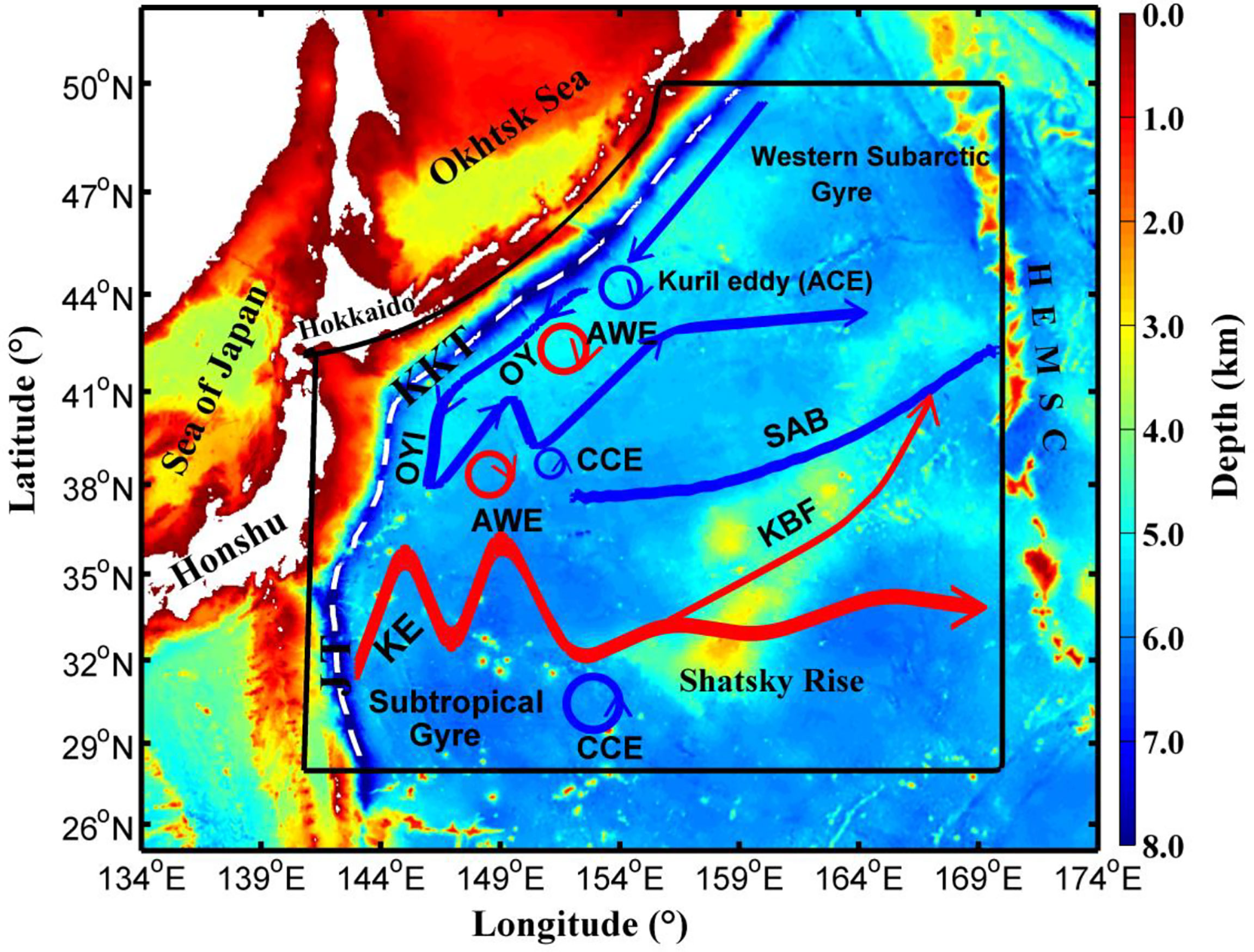
Figure 1 Geography and hydrography of the Kuroshio–Oyashio Extension region (black polygon area). The background color indicates water depth (units: km), and the white dotted line indicates the Japan Trench (JT) and Kuril-Kamchatka Trench (KKT). The symbols “OY”, “OYI”, “KE”, “CCE”, “AWE”, “ACE”, “SAF”, “KBF”, “HEMSC” stand for Oyashio Current, southward intrusion of the Oyashio, Kuroshio Extension, cyclonic cold-core eddy, anticyclonic warm-core eddy, anticyclonic cold-core eddy, Subarctic Front, the Kuroshio Bifurcation Front, and the Hawaii-Emperor Sea mount chain, respectively.

The rest of this work is organized as follows: Section 2 introduces the model data used and the definition method for the four types of mesoscale eddies. Section 3 presents the four eddy cases and their detailed analysis. The statistical differences among the four types of eddies, including the eddy number, radius, vertical penetration depth, seasonal distribution, temperature, salinity, and potential density anomalies modulated by eddies are given in Section 4. In Section 5, we discuss the generation mechanism of abnormal eddies. The conclusions are presented in Section 6.

Data and methodology

OFES data

The model data used in this work are from the Ocean General Circulation Model (OGCM) for the Earth Simulator data (OFES) produced by Japan’s Earth Simulator (Masumoto et al., 2004; Sasaki et al., 2008). The model is based on the Geophysical Fluid Dynamics Laboratory/National Oceanic and Atmospheric Administration (GFDL/NOAA) Modular Ocean Model 3 (MOM3) and improved for parallel computing (Pacanowski and Griffies, 2000). The horizontal spatial resolution is 0.1° × 0.1°, and the calculation area ranges from 75°S to 75°N, covering almost the whole globe except for the Arctic Sea. Vertically, the dataset has 54 layers, and each layer’s interval refers to the thickness of the thermocline layer in the real ocean. The thickness of each layer gradually increases with depth, from 5 m at the surface layer to 330 m at the bottom layer, and the maximum water depth is 6,065 m (Nonaka et al., 2012).

The topography of the model is from the Southampton Marine Centre (provided by GFDL/NOAA) 1/30° resolution ordnance survey data. The horizontal turbulent diffusion term in the momentum equations uses a bi-harmonic operator to suppress the horizontal grid scale error. The model adopts the K-Profile Parameterization (KPP) boundary layer mixing scheme (Large et al., 1994) for vertical mixing. NCEP/NCAR reanalysis data from 1950 to 1999 are used for monthly mean wind stress. The surface heat flux is calculated using the monthly average output of the NCEP/NCAR reanalysis data based on the formula proposed by Rosati and Miyakoda (1988). Masumoto et al. (2004) verified that the OFES data are suited to study large-scale circulation characteristics and mesoscale phenomena by comparing altimeter data.

This study uses the OFES’s sea surface height, meridional and zonal current velocity, temperature, and salinity data from January 2008 – December 2017 provided by the Asia Pacific Data Research Center. The time resolution of the data is three days. By using a band-pass filtering method (please refer to subsection 2.3) to extract mesoscale signals from the OFES dataset, only signals with a spatial scale between 25 – 200 km (Chelton et al., 2011) are retained in this study.

AVISO data

To further confirm the ability of the OFES data to simulate mesoscale phenomena in the KOE region, a new version of the Archiving, Validation, and Interpretation of Satellite Oceanographic (AVISO) data from the same period is used. AVISO integrates a variety of satellite altimeter data to produce results with a spatial resolution of 0.25°×0.25° and a daily temporal resolution (Ducet et al., 2000; Yang et al., 2013; Yang et al., 2015). For more information about the AVISO data, please refer to Pujol et al. (2016).

We use the sea surface geostrophic current anomaly u’ and v’ provided by AVISO to calculate the eddy kinetic energy ($EKE=\frac{u^{\text{'}2}+v^{\text{'}2}}{2}$) and compare it with the EKE calculated from OFES data after band-pass filtering (Figure 2). Figures 2A, B show the same spatial pattern, and both display the existence of the Kuroshio Extension (KE) and Subarctic Front (SAF). That means the band-pass filtered OFES data can accurately identify mesoscale phenomena in the KOE region. The EKE distribution from OFES data (Figure 2A) has more fine-scale structures than that using AVISO data (Figure 2B), and the distribution of SAF is more evident in Figure 2A. This is mainly due to the 0.1° spatial resolution of the OFES data, while that of AVISO data is 0.25°.

FIGURE 2

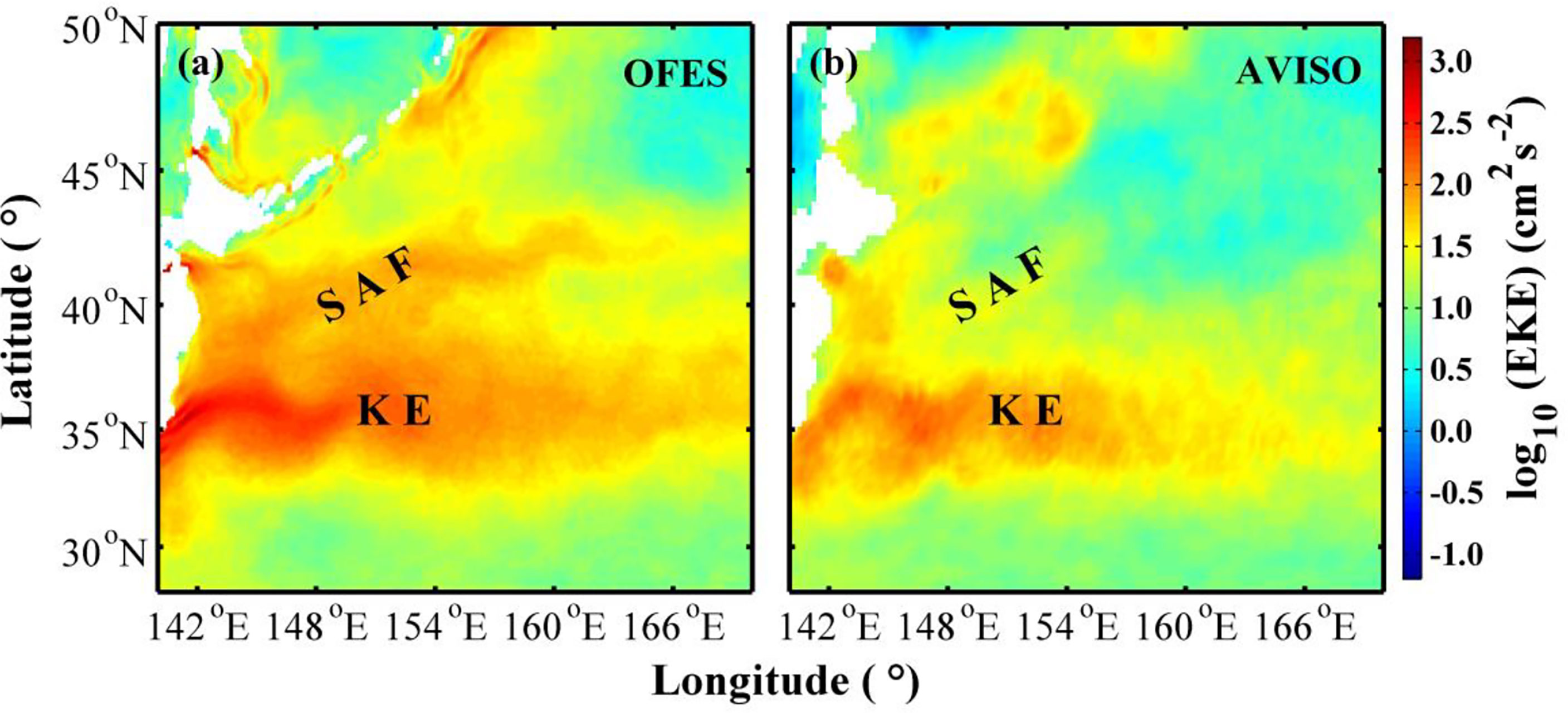
Figure 2 Distribution of sea surface eddy kinetic energy calculated from (A) OFES and (B) AVISO data. Shading indicates the value of eddy kinetic energy (units: cm²/s²). The symbol “KE” and “SAF” represent the Kuroshio Extension and Subarctic Front, respectively. Note that the eddy kinetic energy is plotted with log base 10.

Band-pass filtering method

The band-pass filtering method used in this work includes six steps. The zonal velocity component U(x,y) is used as an example.

Step 1: The spatial average of the two-dimensional current field is subtracted from U(x,y) of the original OFES data to obtain U₁(x,y) .

Step 2: A 200 km low-pass filtering is carried out on U₁(x,y) in the zonal direction to obtain $U_1({\overline{x}}_{200},y)$. The spatial resolution of the OFES data (0.1°) has different spatial distances in the zonal direction at different latitudes (the higher the latitude, the smaller the space). The actual distance varies with latitude as the sampling length of the OFES data during low-pass filtering.

Step 3: $U_1({\overline{x}}_{200},{\overline{y}}_{200})$ is obtained by applying a 200 km low-pass filtering to $U_1({\overline{x}}_{200},y)$ in the meridional direction. In different latitudes, the spatial distance corresponding to a 0.1° resolution in the meridional direction is constant (~ 11.11 km), so the sampling length of the low-pass filter adopts a fixed value here.

Steps 4~5: Similar to steps 2~3, a 25 km low-pass filtering is applied to U₁(x,y) in the zonal and meridional directions to obtain $U_1({\overline{x}}_{25},{\overline{y}}_{25})$.

Step 6: The difference between $U_1({\overline{x}}_{25},{\overline{y}}_{25})$and $U_1({\overline{x}}_{200},{\overline{y}}_{200})$ is taken as the mesoscale signal of U(x,y) after band-pass filtering.

Eddy detection and tracking scheme

There are several automatic eddy detection methods, including the “OW” (Okubo, 1970; Weiss, 1991) and “WA” methods (Sadarjoen and Post, 2000). This study uses the vector geometry-based automatic eddy detection methodology proposed by Nencioli et al. (2010). This method can rapidly detect eddies from any given velocity field and, as such, has been widely applied to many regions (Dong et al., 2012; Liu et al., 2012; Aguiar et al., 2013; Lin et al., 2015; Yang et al., 2020; Sun et al., 2021b; You et al., 2022; Dong et al., 2022). The eddy detection algorithm is applied to the OFES data from January 3, 2008 – December 29, 2017 to detect and track mesoscale eddies.

In order to have more robust results, three additional conditions are imposed on the results obtained from the automatic eddy detection. Firstly, considering that the time scale of the mesoscale eddies is monthly, only eddies surviving for at least 30 days are selected. Secondly, since the spatial scale of the mesoscale eddies is O(100 km) and the spatial resolution of OFES data is 0.1° ×0.1°, only eddies with an average radius larger than 25 km are retained. Thirdly, only eddies with vertical penetration depths of at least 100 m are kept. Please refer to the Appendix for more details concerning the automatic eddy detection and tracking scheme.

Definitions of four types of mesoscale eddies

We divide mesoscale eddies into four types according to the rotation direction of the eddy’s flow field (clockwise or counterclockwise rotation) and the water temperature anomaly (T’) inside the eddy (positive or negative): cyclonic cold-core eddy (CCE, with a counterclockwise rotation flow field and a negative T’), cyclonic warm-core eddy (CWE, with a counterclockwise rotation flow field and a positive T’), anticyclonic warm-core eddy (AWE, with a clockwise rotation flow field and a positive T’), anticyclonic cold-core eddy (ACE, with a clockwise rotation flow field and a negative T’).

The CCEs and AWEs are called normal eddies, while the CWEs and ACEs are named abnormal eddies. Since the abnormal phenomena usually do not occur at all layers, an eddy is regarded as an abnormal eddy as long as there is an abnormal layer vertically. Figures 3A–D give the individual cases of CCE, AWE, CWE, and ACE, respectively. Please refer to the next section for a detailed explanation of these eddy cases.

FIGURE 3

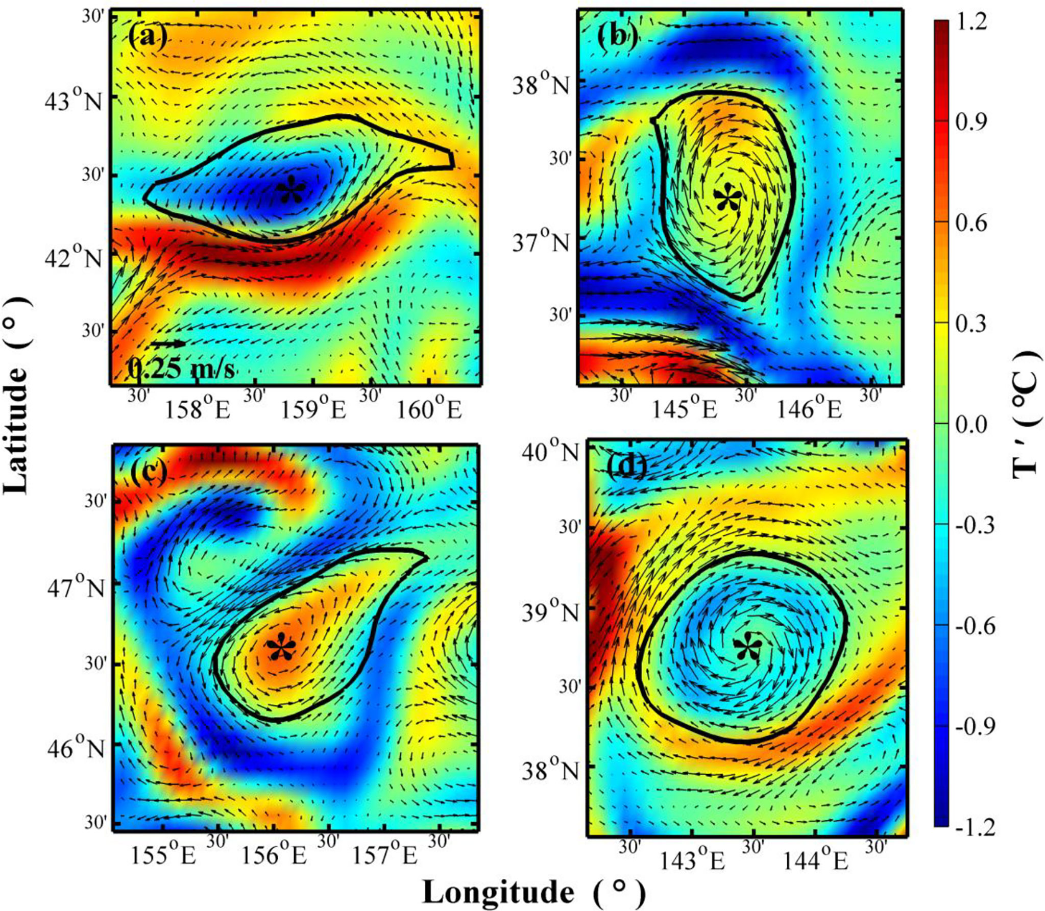
Figure 3 Individual cases of four types of mesoscale eddies. (A) Cyclonic cold-core eddy, (B) anticyclonic warm-core eddy, (C) cyclonic warm-core eddy and (D) anticyclonic cold-core eddy. Black vectors indicate geostrophic current anomalies, bold black curves (black asterisk) indicate the boundary (center) of the eddies, and the background color indicates temperature anomalies (units: °C).

Case Analysis

Basic information on the four types of mesoscale eddy cases

The basic information of the four types of eddy cases shown in Figure 3 is given in Table 1. The CCE case appeared on July 27, 2014 (Figure 3A). Its center is located at (158.65°E, 42.35°N), the average radius is 69.6 km, and its vertical penetration depth is 2,591.6 m. The average T’ inside the CCE case is –0.33°C, and the maximum T’ is –1.03°C. The AWE case shown in Figure 3B appeared on January 2, 2011. The center of the AWE is located at (145.35°E, 37.25°N), the average radius is 62.1 km, and the vertical penetration depth is 1,702.4 m. The average and the maximum T’ inside the AWE is 0.41°C, and 0.96°C, respectively.

TABLE 1

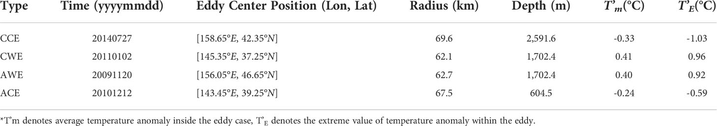
Table 1 Basic information of the four types of eddy cases*.

The CWE case shown in Figure 3C appeared on November 20, 2009. The center of the CWE is located at (156.05°E, 46.65°N), the average radius is 62.7 km, and the vertical penetration depth is 1,702.4 m. The average T’ inside this eddy is 0.40°C, and the maximum T’ is 0.92°C. The ACE case appeared on December 12, 2010 (Figure 3D). The ACE’s center is located at (143.45°E, 39.25°N), the average radius is 67.5 km, and the vertical penetration depth is 604.5 m. The average and the maximum T’ inside the ACE are –0.24°C and –0.59°C, respectively. The average radius of these four eddy cases is about O(60 km), but their vertical penetration depth is significantly different.

Cross-section of temperature, salinity, and potential density anomaly modulated by four types of mesoscale eddy cases

Figure 4 shows the vertical cross-section of temperature anomalies (T’, Figures 4A–D), salinity anomalies (S’, Figures 4E–G, and potential density anomalies σ'_θ, Figures 4I–L) modulated by the four types of mesoscale eddy cases in the upper 1,000 m. There are regular eddy structures in the upper 400 m, with clear closed isotherm lines, and the maximum T’ appears at 45.5 m, reaching –2.56°C(Figure 4A). The CCE case has a significant negative S’ above 200 m (Figure 4E). The maximum negative S’ is –0.28 psu, which appears at 37.8 m. Below 200 m, there is a weak positive S’ but no noticeable closed isohaline lines.

FIGURE 4

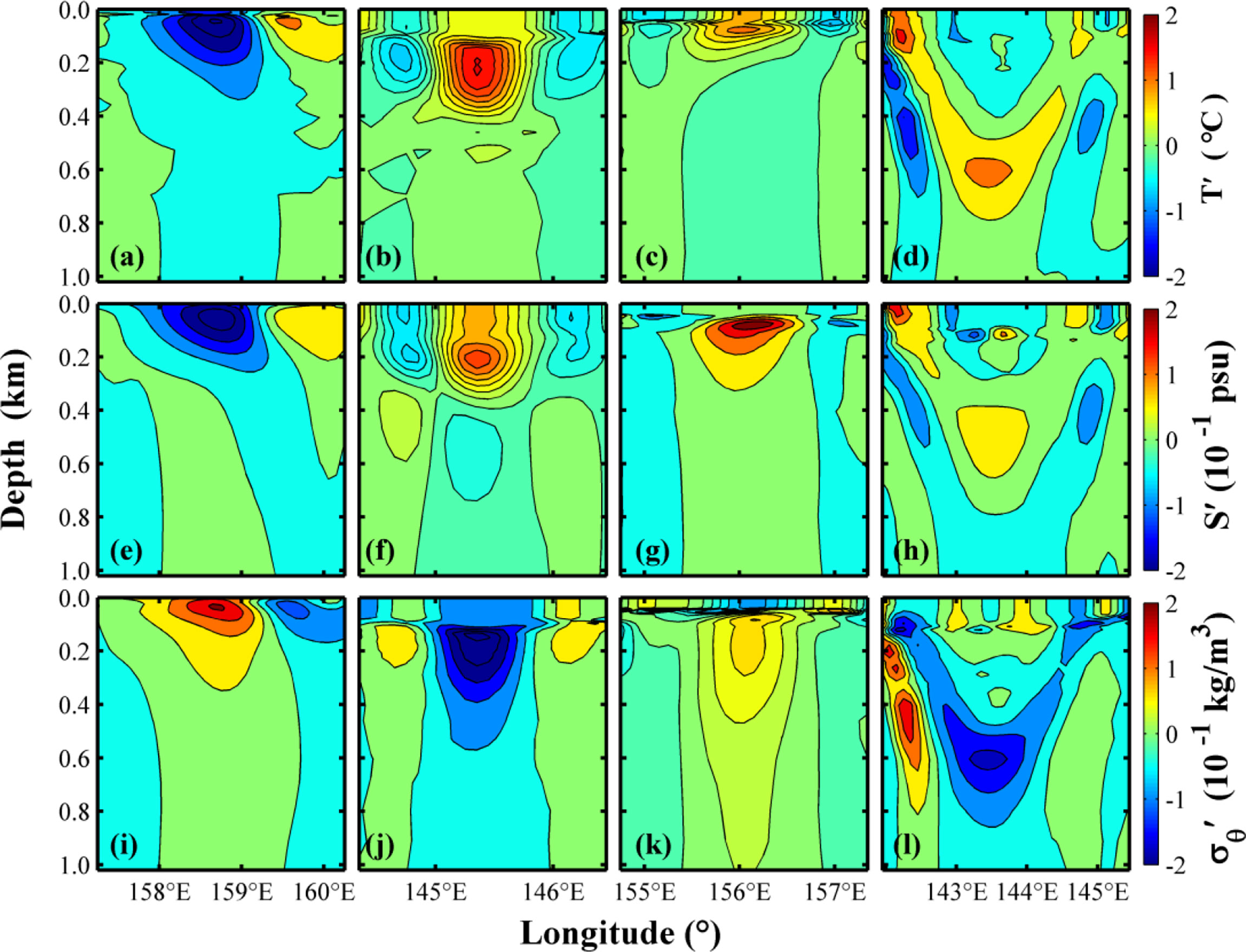
Figure 4 Vertical cross-sections of temperature anomaly (A–D), salinity anomaly (E–H), and potential density anomaly (I–L) are modulated by the four eddy cases. (A, E, I) correspond to the cyclonic cold-core eddy case, (B, F, J) correspond to the anticyclonic warm-core eddy case, (C, G, K) corresponds to the cyclonic warm-core eddy case, and (D, H, L) correspond to the anticyclonic cold-core eddy case. Shading in (A–D), (E–H), and (I–L) indicate temperature (units: °C), salinity (units: 10^-1 psu), and potential density anomalies (units: 10^-1 kg/m³), respectively.

It is known that negative anomalies in temperature (salinity) could induce an (a) increase (decrease) in potential density. From Figure 4I, the potential density anomaly induced by the CCE case presents a positive value, with a maximum of 0.27 kg/m³ occurring at 24.3 m. This indicates that in the case of CCE, the temperature dominates the change in potential density. In addition, from the overall pattern in Figures 4A, E, I, we know that the CCE eddy center shifts about 0.5 degrees to the east within the upper 1,000 m.

Figure 4B shows the vertical temperature cross-section of an AWE case. The sea water temperature inside the AWE case is generally warm. Furthermore, the T’ is small in the upper 100 m (approximately the depth of the mixed layer), only about 0.5°C. There is a distinct isotherm line closed ring structure between 100 and 400 m. The maximum T’ appears at 223.2 m (reaching 1.64°C). After analysis, the maximum T’ depth is close to the position of the main thermocline. It can be inferred that the AWE case is in the form of the first baroclinic mode in the vertical direction. That is, T’is the largest at the main thermocline and decreases rapidly at other positions.

The AWE-induced S’ has an apparent two-layer structure (Figure 4F). Above 400 m, it corresponds to a positive S’ with a maximum value of 0.14 psu, which occurs at 192.5 m. Similar to T’, S’ changes slightly and evenly within the upper 200 m. A weak negative S’ appears below 400 m, and the maximum value appears at 460.5 m, reaching –0.09 psu. The positive T’ above 400 m induces a negative σ'_θ, and the positive S’ induces a positive σ'_θ. However, σ'_θ of the AWE case is always negative (Figure 4J). Therefore, temperature dominates the change in potential density in the AWE case. Both positive T’ and negative S’ induce negative σ'_θbelow 400 m, but because their changes are very weak, so the σ'_θis very small as well. The maximum change in potential density occurs at 148.4 m, reaching –0.27 kg/m³. In addition, it can be seen from Figures 4B, F, J that the AWE center is not offset in the vertical direction.

The CWE corresponds to a positive T’ within the upper 300 m, with a maximum of 1.09°C at 73.2 m (Figure 4C). Below 300 m, it corresponds to a negative T’, with the maximum anomaly reaching –0.19°C at 460.5 m. Therefore, the CWE case belongs to an abnormal eddy within the upper 300 m and is a normal eddy below that depth. As shown in Figure 4G, this CWE case has a pronounced S’ above 400 m, with the maximum S’ of 0.24 psu appearing at 84.0 m. There is an apparent high S’ core between 50 and 400 m. The salinity variation above 50 m and below 400 m is very weak, and the variation range is only about 0.02 psu.

From the distribution of σ'_θ (Figure 4K), it can be seen that above 50 m, T’ dominates the variation of potential density and induces a negative value. The maximum value (reaching –0.09 kg/m³) appears at 24.3 m. Below 50 m, S’ dominates the variation of potential density and induces a positive σ'_θ. The maximum value appears at 207.5 m, reaching 0.08 kg/m³. Different factors control the variation of σ'_θ in different layers of the CWE case, with temperature dominating in the upper layers and salinity in the lower layers. The CWE center also does not incline in the vertical direction.

The vertical temperature cross-section of the ACE case is shown in Figure 4D. On the whole, the cross-section shows a two-part structure. One is the positive T’ at the ACE boundary, and the other is the negative T’ inside the eddy. The positive T’ displays a wine cup-shaped eddy boundary, where the wine cup contains seawater with a negative T’. The largest T’ in the cup-shaped eddy structure occurs at 604.5 m, and T’ reaches 1.26°C. The temperature of the relatively cold water in the ACE case is relatively uniform, and the change range is not obvious, with an average of –0.20°C.

Figure 4H shows that the S’ is consistent with T’. The wine cup-shaped eddy boundary corresponds to an obvious positive S’. The maximum anomaly at the eddy center reaches 0.11 psu at 604.5 m, while the seawater inside shows a weak negative S’, with an average value of 0.01 psu.

Concerning σ'_θ, the wine cup-shaped eddy boundary structure and the seawater inside the eddy show that the temperature change dominates potential density. The maximum σ'_θ occurs at 604.5 m, reaching –0.18 kg/m³. From the T’ at the ACE boundary, the eddy is a normal eddy, but from the T’ within the eddy, the eddy is abnormal. The ACE center is also not inclined vertically.

Based on the analysis of these eddy cases, it can be seen that temperature, salinity, and potential density anomaly modulated by normal eddies are more significant than those modulated by corresponding abnormal eddies. Additionally, a normal eddy shows a uniform cold or warm anomaly in the vertical direction. The anomalous phenomena of abnormal eddies are concentrated in the ocean’s upper layer, while it often disappears at a deeper level, where abnormal eddies change back to normal eddies.

Statistical characteristics analysis of the four types of mesoscale eddies

Horizontal distribution of the four types of mesoscale eddies

Figure 5 shows the horizontal distribution of the four types of eddy numbers in each 1° by 1° grid. The number of CCEs (10,471) accounts for 38.46% of the total eddies (Figure 5A). The maximum number of CCEs in a single grid is 59, which appears at (161°E, 41°N). Figure 5B shows the number of AWEs (9,841), accounting for 36.15% of the total eddies. The maximum value in a single grid is 86, which appears at (156°E, 44°N). Comparing Figures 5A, B, the distribution of CCEs and AWEs are roughly the same, and the number of CCEs is 6.40% more than that of AWEs. CCEs and AWEs are evenly distributed in the meridional direction, and the higher the latitude, the larger the number of eddies. The large CCEs and AWEs number areas are concentrated in the open ocean, while it is relatively small along the coast.

FIGURE 5

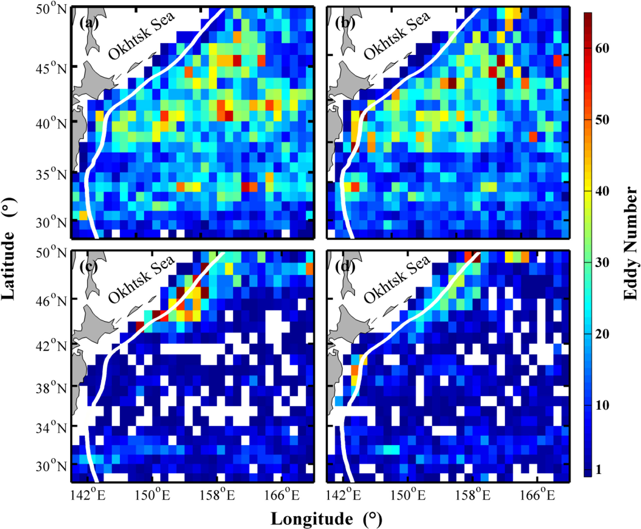
Figure 5 Spatial distribution of the four types of eddy numbers in 1° × 1° grids in the Kuroshio-Oyashio Extension region from January 3, 2008 – December 29, 2017. Subplots (A–D) give the cyclonic cold-core, anticyclonic warm-core, cyclonic warm-core, and anticyclonic cold-core eddies, respectively. Shading represents eddy number (areas with no eddies are shown in white). The bold white curve represents Japan and the Kuril-Kamchatka Trenches.

The distribution of the number of CWEs is shown in Figure 5C. The number of CWEs is 3,647, accounting for 13.40% of the total eddies. The maximum number of CWEs in a single grid is 155, located at (154°E, 47°N), near the Okhotsk Sea. Figure 5D shows the distribution of ACEs in 1°by 1° grids, with 3,267 accounting for 11.99% of the total eddies. The maximum number of ACEs in a single grid is 65 (159°E, 42°N), also located near the Okhotsk Sea. By comparing Figures 5C, D, it can be seen that CWEs and ACEs are mainly distributed at the edge of the KOE region, mostly along the Kuril-Kamchatka Trench. The number of abnormal eddies in the open ocean is relatively small, with no abnormal eddies detected in several grids (white patches in Figures 5C, D).

Abnormal eddies are unevenly distributed in space (mostly concentrated in the continental shelf boundary region), while normal eddies are primarily concentrated in the open ocean. The number of CWEs and ACEs is 34.83 and 33.20% of CCEs and AWEs, respectively. The number of ACEs is 10.42% less than that of CWEs. In conclusion, the number of abnormal eddies (6,914) in the KOE region is about 34.04% of normal eddies (20,312). This proportion is much higher than the results of Sun et al. (2019), but it is very close to Liu et al. (2021). The main reason for this difference with Sun et al. (2019) is the different definitions of abnormal eddies.

Vertical distribution of the number of the four types of mesoscale eddies

In order to have a clear understanding of the vertical distribution of the four types of eddy numbers, a ratio (R₁) between the four types of eddy numbers at each layer to the number of surface eddies is calculated as:

$\begin{array}{ll}{R}_1\left(z\right)=\frac{N_i}{N_1},i=1,2,3,\mathrm{\dots 54}& (1)\end{array}$

where N₁represents the number of eddies in layer i and N₁ represents the number of eddies in the surface layer.

Figure 6 shows the vertical distribution of R₁(z) . Within the upper 100 m, R₁ is always equal to one due to the additional restriction that the vertical penetration depth of the eddy is at least 100 m. When the water depth reaches 1,000 m, the corresponding R₁ of CCEs, AWEs, CWEs, and ACEs is 36.03, 11.92, 0.32, and 0.24%. At 2,000 m, R₁ for CCEs, AWEs, CWEs, and ACEs is 9.16, 1.31, 2.91, and 0.70%, respectively. Here, the number of eddies decreases rapidly with increasing depth. The downward trend of R₁ is another representation of the vertical penetration depth of the eddy (please refer to Figure 7). Therefore, it is necessary to consider at least 2,000 m to discuss the impact of eddies when analyzing the vertical distribution of eddy numbers, especially for normal eddies.

FIGURE 6

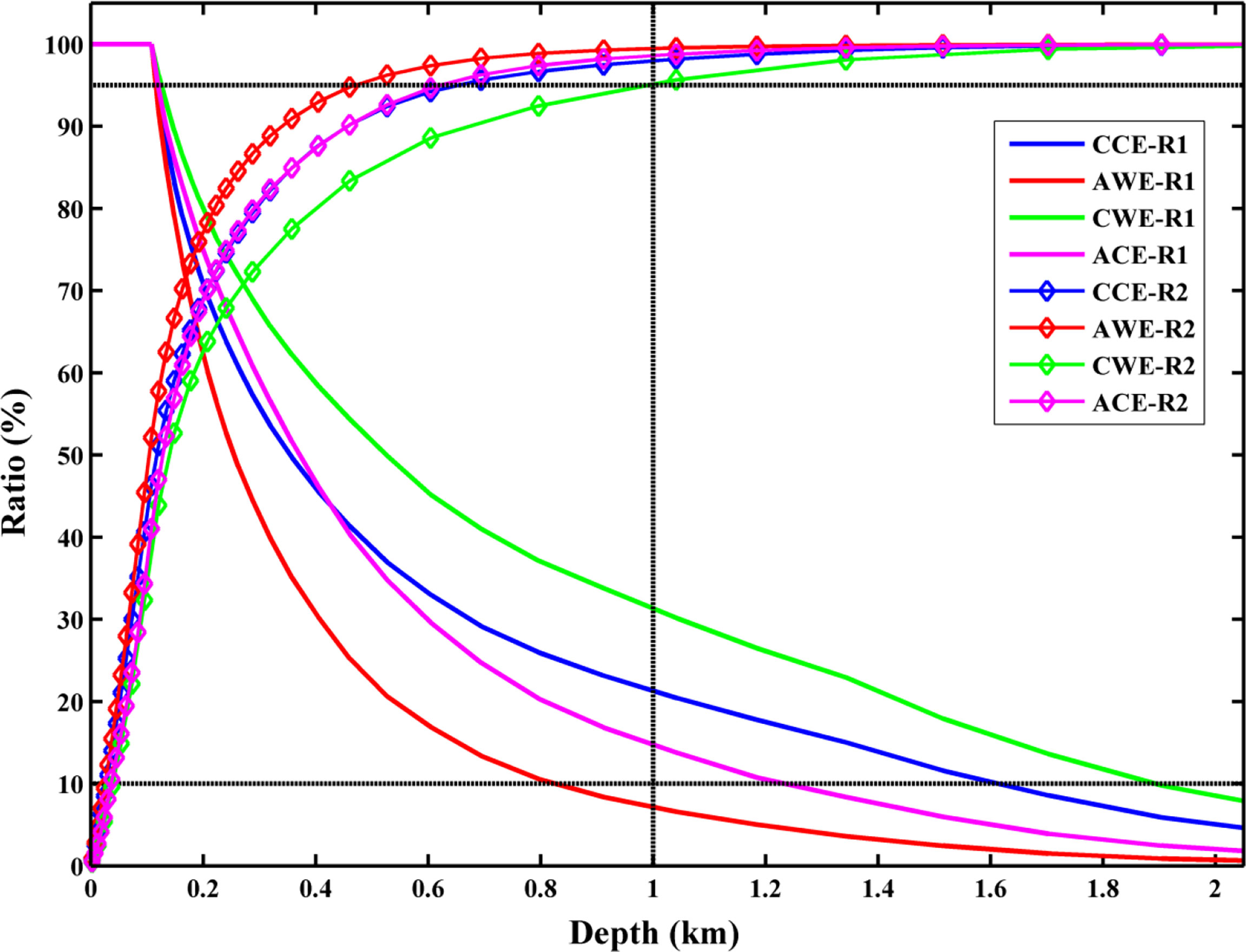
Figure 6 Ratio R₁ distribution of the number of four types of eddies at different depths to the total number of surface layer eddies (solid lines), and ratio R₂ distribution of the cumulative heat content in the vertical direction to the total heat content (diamond lines). The vertical black dotted line represents 1,000 m, and the horizontal black dotted lines represent 10% and 95% isobaths, respectively.

FIGURE 7

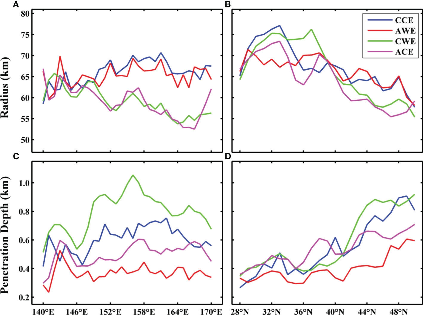
Figure 7 Variation of average eddy radius and vertical penetration depth of three-dimensional eddies with (A, C) longitude and (B, D) latitude. The figure’s blue, red, green, and magenta lines indicate cyclonic cold-core, anticyclonic warm-core, cyclonic warm-core, and anticyclonic cold-core eddies, respectively.

However, previous studies have shown that eddy-induced effects are mainly concentrated in the upper 1,000 m of the ocean (Dong et al., 2017). In order to further illustrate this point, we calculate the vertical distribution of the cumulative ratio (R₂ ) of heat content anomaly within the eddies:

$\begin{array}{ll}{R}_2\left(z\right)=\frac{{\sum }_{i=1}^n{Q}_n}{{\sum }_{i=1}^{53}{Q}_i},n=1,2,3,\dots ,53.& (2)\end{array}$

where R₂(z) represents the ratio of accumulated heat content anomaly to total heat anomaly, n=1,2,3,…,53 , $Q_n= c_{\rho }\rho \pi r_{n}2\frac{d_{n+1}-d_n}{2}\left|T_n^{\text{'}}\right|$, c_ρ is the specific heat capacity of seawater, ρ is the density of seawater, r_n is the average radius of the eddy at this level. d_n represents the depth of the current layer and $T_n^{\text{'}}$ represents the corresponding temperature anomaly inside the eddy at the current level.

From Figure 6, in the upper layer, the proportion of heat content anomaly in the four types of eddies increases rapidly with the increase in depth. At 1,000 m, R₂ for CCEs, AWEs, CWEs, and ACEs is 97.83, 99.41, 94.89, and 98.49%. Similarly, at 2,000 m, R₂ is 99.91, 99.99, 99.74, and 99.96%, respectively. From the perspective of eddy-induced heat content anomalies, the impacts of the eddies are mainly concentrated within the upper 1,000 m.

Distribution of average eddy radius and vertical eddy penetration depth

Figure 7 shows the variation of the average eddy radius (Figures 7A, B) and vertical penetration depth (Figures 7C, D) of the three-dimensional eddy with longitude (Figures 7A, C) and latitude (Figures 7B, D). Figures 7A, B show that the average radius of CCEs and AWEs is 65.96 ± 2.86 and 65.28 ± 2.38 km, respectively, with little difference between them. The average eddy radius of both CCEs and AWEs tends to increase gradually from the coast to the open ocean (Figure 7A). On the contrary, the average eddy radius of CWEs is 59.11 ± 3.98 km, and that of ACEs is 58.88 ± 4.88 km.

In the western part of the North Pacific Ocean near the continental shelf area (140°E – 150°E), there is no obvious difference between the average radius of normal and abnormal eddies. However, in the open ocean, the average radius of normal eddies is significantly larger than that of abnormal eddies. This difference may be because the abnormal eddies mainly occur in the formation and decay stages of the eddies’ lifespan when their radius are relatively small (Sun et al., 2019). The terrain near the western boundary limits the growth of eddies, making the eddy radii relatively small. On the other hand, eddies generated in the open ocean also tend to move westward and decay in those boundary regions, resulting in a relatively small average eddy radius. The average eddy radius of the four types of eddies tends to decrease with the increase in latitude (Figure 7B). This variation may be caused by the gradual decrease of the first baroclinic Rossby deformation radius with an increase in latitude (Sun et al., 2021b).

The average vertical penetration depth of CCEs, AWEs, CWEs, and ACEs is 604.94 ± 91.08, 370.63 ± 52.00, 797.11 ± 153.33, and 499.12 ± 104.07 m, respectively. Normal eddies’ vertical penetration depth is consistent with the variation trend along the longitude (Figure 7C) and latitude (Figure 7D), but both are shallower than the corresponding abnormal eddies. The vertical penetration depth of AEs is shallower than that of CEs (Figure 7C, D). In the zonal direction, the average penetration depth of eddies in the open ocean is deeper than that in the marginal area, especially for CWEs. Meridionally, the vertical penetration depth of the four types of eddies increases significantly with the increase in latitude.

Seasonal distribution of the four types of eddy numbers

Figure 8 shows the seasonal distribution of the number of four types of eddies. The variation trend of normal eddies is consistent as a whole, i.e., there is no noticeable difference in the number of CCEs and AWEs. Both are characterized by a large number in winter months (December – February) and a small number in summer months (June – August). The largest number occurred in January, with 1,341 CCEs and 1,308 AWEs. The minimum eddy number appears in May (672) for CCEs and in July (590) for AWEs.

FIGURE 8

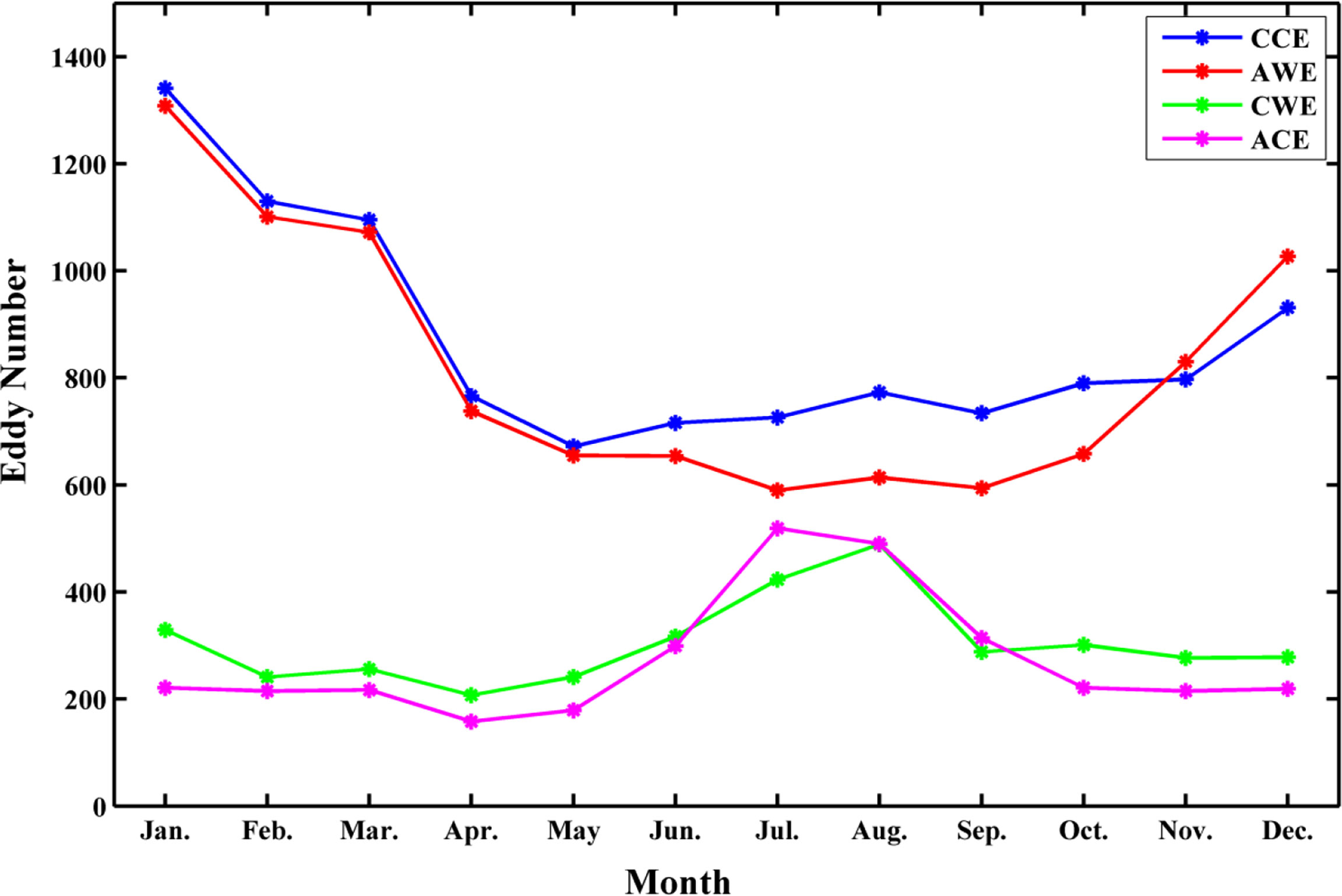
Figure 8 Seasonal distribution of the four types of eddy numbers. The blue, red, green, and magenta lines represent cyclonic cold-core, anticyclonic warm-core, cyclonic warm-core, and anticyclonic cold-core eddies, respectively.

The overall variation trends of CWEs and ACEs are also very similar, showing more eddies in summer and autumn than in winter and spring. The maximum and the minimum value of CWEs appear in August (489) and February (241), respectively. Accordingly, the maximum and the minimum number of ACEs appear in July (519) and April (158). Therefore, the number of normal and abnormal eddies shows the opposite seasonal trends. This distribution may be because the sea surface wind stress curl in the KOE region is intense in winter (figure not shown). The wind-induced eddies in winter are not only numerous but also substantial, making it challenging to generate abnormal eddies. In summer, due to the relatively weaker wind stress curl, the abnormal eddy phenomenon is more likely to occur in the ocean’s upper layer (Ni et al., 2021).

Eddy-induced temperature, salinity, and potential density anomalies

Previous studies pointed out that mesoscale eddies can cause vertical anomalies of various marine elements (Gaube et al., 2019). Figure 9 shows the vertical distribution of temperature, salinity, and potential density anomalies modulated by the four types of eddies. Figures 9A–C show the result within a one-time eddy radius, and Figures 9D–F show the situation within 0.5 times eddy radius. The vertical changes of T’ modulated by normal eddies are consistent (Figures 9A, D). CCEs induce a negative T’ (Figure 9A). For the results within a one-time the radius (0.5 times the radius), the maximum value of CCEs-modulated T’ is -0.78°C (-1.48°C), which occurs at 63.23 m (120.77 m). Accordingly, AWEs induce a positive T’ (Figure 9A). For the result within a one-time radius (0.5 times radius), the maximum T’ is 0.74°C (1.32°C) at 63.23 m (63.23 m).

FIGURE 9

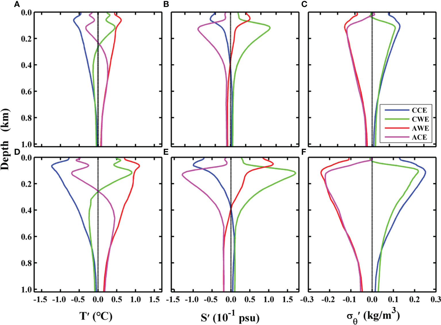
Figure 9 Vertical distribution of the four types of eddies-modulated temperature (A, D, units: °C), salinity (B, E, units: 10^-1 psu), and potential density anomalies (C, F, units: kg/m³). Subfigures (A–C) show the results averaged within a one-time eddy radius, and (D–F) show the results averaged within 0.5 times eddy radius. The blue, red, green, and magenta lines represent cyclonic cold-core, anticyclonic warm-core, cyclonic warm-core, and anticyclonic cold-core eddy, respectively.

CWEs induce a positive T’ at the ocean’s upper 250 m (Figure 9A). For the result within a one-time radius (0.5 times radius), the maximum T’ is 0.54°C (1.08°C) and occurs at 120.77 m (120.77 m). A negative T’ is modulated by CWEs below 250 m, the same as CCEs. ACEs induce a negative T’ at the ocean’s upper 250 m (Figure 9A). For the result within one-time of the radius (0.5 times of the radius), the maximum value of T’ is -0.39°C (-0.84°C), which occurs at 120.77 m (120.77 m). ACEs induce a positive T’ below 250 m, similar to AWEs.

To summarize, T’ modulated by abnormal eddies has a two-layer structure. At about 250 m, the abnormal eddies-modulated T’ changes sign. Specifically, T’ modulated by the CWEs is warmer in the upper 250 m and colder below that depth. In contrast, T’ modulated by ACEs is colder in the ocean’s upper 250 m and warmer below that depth. The abnormal eddy phenomenon is mostly concentrated in the upper layer of the ocean, which can also be verified from the vertical distribution of abnormal eddy numbers (Figure 6). Generally, the temperature changes modulated by abnormal eddies are weaker than those modulated by normal eddies.

Figures 9B, E show the vertical distribution of eddies-modulated S’ within one-time of the eddy radius (Figure 9B) and 0.5 times of the eddy radius (Figure 9E). The salinity anomaly modulated by normal eddies shows a two-layer structure. Above (below) about 400 m, the CCEs induce a negative (positive) S’. Under the one-time eddy radius (0.5 times eddy radius), the maximum CCEs-modulated S’ is –0.05 psu (–0.10 psu), which occurs at 54.02 m (63.23 m). Accordingly, the maximum S’ modulated by AWEs, CWEs, and ACEs is 0.05 (0.11), 0.10 (0.17), and –0.08 psu (–0.13 psu), which occurs at 45.56 (45.56), 120.77 (120.77), and 134.31 m (134.31 m), respectively.

From Figures 9A, B, D, E, contrary to T’, the variation amplitude of S’ modulated by abnormal eddies is more significant than that of normal eddies. Salinity anomalies modulated by CCEs and AWEs (CWEs and ACEs) are symmetrically distributed. The depth of maximum S’ modulated by abnormal eddies is larger than those modulated by normal eddies.

The vertical distribution of eddies-modulated σ'_θ within one-time and 0.5 times the eddy radius is shown in Figures 9C, F, respectively. Potential density anomalies modulated by the four types of eddies show the same structure from top to bottom. CEs (including CWEs and CCEs) induce a positive σ'_θ, and AEs (including ACEs and AWEs) induce a negative σ'_θ. Under the one-time eddy radius (0.5 times eddy radius), the maximum σ'_θ modulated by CCEs is –0.05 kg/m³ (–0.10 kg/m³), which occurs at 54.02 m (63.23 m). Accordingly, the maximum σ'_θ modulated by AWEs, CWEs, ACEs is 0.05 (0.11), 0.10 (0.17), and –0.08 kg/m³ (–0.13 kg/m³) which occurs at 45.56 (45.56), 120.77 (120.77), and 134.31 m (134.31 m), respectively.

Several observations can be made from the above analysis. Firstly, the changing trend of σ'_θ modulated by normal eddies is the same as that of T’. Specifically, taking the CCEs (AWEs) as an example, the T’ modulated by the CCEs (AWEs) is negative (positive), which increases (decreases) potential density. In contrast, S’ modulated by the CCEs (AWEs) is negative (positive), which decreases (increases) potential density. However, from Figure 9C, σ'_θ modulated by the CCEs (AWEs) is positive (negative). Therefore, the CCEs-modulated(AWEs-modulated) potential density anomaly is dominated by temperature.

Secondly, the changing trend of σ'_θ modulated by abnormal eddies is opposite to that of T’. Specifically, taking CWEs (ACEs) as an example, T’ modulated by CWEs (ACEs) above 250 m is positive (negative), which reduces (increases) the potential density. The CWEs-modulated (ACEs-modulated) S’ is positive (negative), which increases (decreases) the potential density. The σ'_θ modulated by CWEs (ACEs) is positive (negative) from Figure 9F. Therefore, the change in potential density modulated by CWEs (ACEs) is dominated by salinity.

Thirdly, σ'_θ modulated by CEs and AEs are almost symmetrically distributed. Fourthly, the pattern of σ'_θ modulated by normal and abnormal eddies is the same. However, in the upper layer, the normal eddies-modulated σ'_θ is much larger than that modulated by abnormal eddies. Lastly, the σ'_θ modulated by abnormal eddies within the upper 50 m is almost zero.

Discussion

The discussion on the generation mechanism can deepen our understanding of mesoscale eddy dynamics. Current generation mechanisms of abnormal eddies mainly focus on analyzing individual cases of eddies. The primary generation mechanisms reported in the literature include the following.

(1) Abnormal eddies are generated due to the influence of the surrounding hydrological environment. Itoh and Yasuda (2010a) pointed out many ACEs around the Oyashio southward intrusions and farther north near the Kuril Islands. Based on the heat content anomaly integrated over 50 ~ 200 dbar, 15% of the AEs within 35°N ~ 50°N, 140°E ~ 155°E have a cold and fresh core. There are two processes for forming ACEs in that area: direct formation from the cold, freshwater outflow from the Okhotsk Sea, and modification of AWEs that originate from the Kuroshio Extension. In addition, if the eddy nonlinearity is less than one, i.e., the AWE propagation velocity exceeds the rotation velocity at a certain depth, then the eddy core water is replaced by ambient cold water that will form an ACE (Flierl, 1981).

Similarly, a particular hydrological environment also exists in the SCS. The difference is warm Kuroshio water in the periphery of the SCS. After the Kuroshio intrudes into the SCS, a CE pinches off the central axis of the Kuroshio, containing warmer water than the surrounding area and forms a CWE. The interior of this CWE is warm water from the Kuroshio and the eddy exterior is cold water from the SCS. On the contrary, if an AE is generated after the meandering of the Kuroshio’s central axis entraps relatively cold water, an ACE will be formed (Sun et al., 2021a).

(2) The instability of the eddy itself leads to the generation of abnormal eddies. Sun et al. (2019) pointed out that eddies lose their coherent structure in the decay stage, become very unstable, and generate abnormal eddies. They found that a CCE’s radius suddenly increases and absorbs warm waters from the ambient area, which turns this CCE into a CWE.

(3) The interaction between eddies leads to the formation of abnormal eddies. Based on satellite observation data in the North Pacific Ocean, Sun et al. (2019) found that the interaction between adjacent eddies can entrain cold water into the interior of an AWE, thus generating an ACE.

(4) The interaction between eddy and wind generates abnormal eddies. Specifically, the relative motion between the wind and the eddy surface current causes Ekman pumping. That is, the upwelling (sinking) of the isopycnal within the AEs (CEs) (McGillicuddy et al., 2007; Gaube et al., 2015; McGillicuddy, 2015) to finally generate abnormal eddies. Through the global abnormal eddy phenomenon analysis, Ni et al. (2021) confirmed that this mechanism plays a vital role in the tropical region.

(5) AEs influence the barrier layer and lead to abnormal eddies. By analyzing more than a decade of in situ, satellite, and reanalysis data, He et al. (2020) showed that AEs could significantly thicken the barrier layer in salinity-stratified oceans in winter. This thickening of the barrier layer consists of the isothermal layer’s deepening, which then inhibits the upward heat supply into the mixed layer and retains the heat in the barrier layer. On the other hand, it shoals the mixed layer and promotes winter surface cooling and subsurface temperature inversion. Under the joint action of these two aspects, sea surface temperature is lower in the AEs compared to the ambient region and thus generates ACEs.

In summary, many mechanisms could lead to abnormal eddies. Therefore, specific to each abnormal eddy, it may have its characteristics or a variety of mechanisms acting together to generate it. Establishing a standard for automatic abnormal eddies classification generated under different generation mechanisms requires further study.

Conclusions

The KOE region is characterized by the most substantial air-sea interaction and mesoscale eddy activity in the North Pacific Ocean. This work divides eddies into four types and performs detailed analyses of their characteristics to deepen understanding eddy phenomenon in this area.

Based on case studies, the central axis of some eddies in the KOE area is tilted in the vertical direction. It is also found that the temperature anomaly modulated by the normal eddies is more significant than that modulated by abnormal eddies. On the contrary, the abnormal eddies-modulated salinity anomaly is larger than that of normal eddies. Moreover, abnormal eddies are concentrated in the ocean’s upper layer, while they often turn to normal eddies again in the deeper ocean.

Based on statistical analyses, the number of CCEs (10,471), AWEs (9,841), CWEs (3,647), and ACEs (3,267) at the sea surface account for 38.46, 36.15, 13.40, and 11.99% of the total number of eddies, respectively. That is, the number of abnormal eddies (6,914) is about 34.04% of the number of normal eddies (20,312). CCEs and AWEs are mainly concentrated in the open ocean and relatively scarce in the coastal boundary area. By contrast, CWEs and ACEs are mainly distributed at the edge of the KOE region.

In the vertical direction, the number of four types of eddies decreases rapidly with the increase in depth. Eddies’ effects are within about 2,000 m considering the eddy number. However, eddy-modulated heat content anomalies account for more than about 95% of the total heat content anomalies within the upper 1,000 m. The average eddy radius for CCEs, AWEs, CWEs, and ACEs is 65.96 ± 2.86, 65.28 ± 2.38, 59.11 ± 3.98, and 58.88 ± 4.88 km, respectively. In the zonal direction, the average radius of normal eddies gradually increases from the coastal area to the open ocean.

Along the KOE shelf area (140°E – 150°E), there is no significant difference between the average radius of abnormal and normal eddies. In the open ocean, by contrast, the average eddy radius of normal eddies is larger than that of abnormal eddies. In the meridional direction, the average eddy radius of the four types of eddies decreases gradually with the increase in latitude. The average vertical penetration depth of CEs is larger than that of AEs. Normal eddies’ vertical penetration depth is shallower than the corresponding abnormal eddies. In the zonal direction, the average penetration depth of the four types of eddies is deeper in the open ocean than in the marginal sea, while in the meridional direction, the eddies penetrate deeper as latitude increases.

The distribution in different months shows that the normal eddies mainly occur in winter and spring, while the abnormal eddies are mainly concentrated in summer and autumn. Temperature anomalies modulated by normal eddies show a consistent trend in the vertical. However, abnormal eddies-modulated T’ shows a two-layer structure, with positive (negative) T’ associated with CWEs (ACEs) at upper 250 m and negative (positive) T’ below that depth.

Temperature changes modulated by abnormal eddies are smaller than those modulated by normal eddies. However, the variation range of abnormal eddies-modulated S’ is larger than that of normal eddies. The depth of abnormal eddies-modulated maximum S’ is deeper than that modulated by normal eddies.

The density anomalies modulated by the four types of eddies show the same structure from top to bottom. CEs induce positive σ'_θ, and AEs induce negative σ'_θ. The potential density anomaly modulated by CCEs (AWEs) is dominated by temperature. However, the σ'_θ modulated by CWEs (ACEs) is dominated by salinity.

The discovery of abnormal eddies enriches the research content of eddy dynamics. The detailed discussion of the four types of eddies in the KOE region helps deepen the understanding of regional oceanography. It is also helpful to establish more refined maritime weather forecasts that consider the influence of mesoscale eddies on atmospheric variables. In addition, heat and material transports modulated by eddies, especially the transports modulated by abnormal eddies and their generation mechnisms, are worthy of further investigation.

Data Availability Statement

The datasets presented in this study can be found in online repositories. The names of the repository/repositories and accession number(s) can be found in the article/Supplementary Material.

Author contributions

WS, CD, and YL conceived and designed the experiments. WS performed the experiments. WS, MA, JL, JL, and WT analyzed the data. WS drafted the original manuscript, and CD, YL, and JY revised and edited the manuscript. All authors contributed to the article and approved the submitted version.

Funding

National Natural Science Foundation of China under contract Nos. 41906008, 42192562, 42076162, 42176012; Open Fund of State Key Laboratory of Satellite Ocean Environment Dynamics, Second Institute of Oceanography, MNR under contract No. QNHX2231; the Natural Science Foundation of Guangdong Province of China under contract No. 2020A1515010496; and the Innovation Group Project of Southern Marine Science and Engineering Guangdong Laboratory (Zhuhai) under contract No. 311020004.

Acknowledgments

The authors thank Brandon J. Bethel and Kenny T.C. Lim Kam Sian for the English language editing. The altimeter products are produced by the Ssalto/Duacs and distributed by AVISO, with support from the Centre National d’Etudes Spatiales (http://www.aviso.oceanobs.com/duacs/). The OFES data are downloaded from http://apdrc.soest.hawaii.edu/dods/public_ofes/OfES. We thank the editor (Prof. Wang Qiang) and two anonymous reviewers for their constructive comments and helpful suggestions on an earlier manuscript version.

Conflict of interest

The authors declare that the research was conducted in the absence of any commercial or financial relationships that could be construed as a potential conflict of interest.

Publisher’s Note

All claims expressed in this article are solely those of the authors and do not necessarily represent those of their affiliated organizations, or those of the publisher, the editors and the reviewers. Any product that may be evaluated in this article, or claim that may be made by its manufacturer, is not guaranteed or endorsed by the publisher.

Supplementary material

The Supplementary Material for this article can be found online at: https://www.frontiersin.org/articles/10.3389/fmars.2022.984244/full#supplementary-material

References

Adams K. A., Hosegood P., Taylor J. R., Sallée J., Bachman S., Torres R., et al. (2017). Frontal circulation and submesoscale variability during the formation of a southern ocean mesoscale eddy. J. Phys. Oceanogr. 47 (7), 1737–1753. doi: 10.1175/JPO-D-16-0266.1

CrossRef Full Text | Google Scholar

Aguiar A. C. B., Peliz Á., Carton X. (2013). A census of meddies in a long-term high-resolution simulation. Prog. Oceanogr. 116 (9), 80–94. doi: 10.1016/j.pocean.2013.06.016

CrossRef Full Text | Google Scholar

Archer M., Schaeffer A., Keating S., Roughan M., Holmes R., Siegelman L. (2020). Observations of submesoscale variability and frontal subduction within the mesoscale eddy field of the Tasman Sea. J. Phys. Oceanogr. 50 (5), 1509–1529. doi: 10.1175/JPO-D-19-0131.1

CrossRef Full Text | Google Scholar

Bishop S. P., Bryan F. O. (2013). A comparison of mesoscale eddy heat fluxes from observations and a high-resolution ocean model simulation of the kuroshio extension. J. Phys. Oceanogr. 43 (12), 2563–2570. doi: 10.1175/JPO-D-13-0150.1

CrossRef Full Text | Google Scholar

Castelao R. M. (2014). Mesoscale eddies in the south Atlantic bight and the gulf stream recirculation region: Vertical structure. J. Geophys. Res. 119, 2048–2065. doi: 10.1002/2014JC009796

CrossRef Full Text | Google Scholar

Chaigneau A., Gizolme A., Grados C. (2008). Mesoscale eddies off Peru in altimeter records: Identification algorithms and eddy spatiotemporal patterns. Prog. Oceanogr. 79 (2), 106–119. doi: 10.1016/j.pocean.2008.10.013

CrossRef Full Text | Google Scholar

Chaigneau A., Texier M. L., Eldin G., Grados C., Pizarro O. (2011). Vertical structure of mesoscale eddies in the eastern south pacific ocean: A composite analysis from altimetry and argo profiling floats. J. Geophys. Res. 116 (C11025), 476–487. doi: 10.1029/2011JC007134

CrossRef Full Text | Google Scholar

Chelton D. B. (2013). Ocean-atmosphere coupling: Mesoscale eddy effects. Nat. Geosci. 6 (8), 594–595. doi: 10.1038/ngeo1906

CrossRef Full Text | Google Scholar

Chelton D. B., Schlax M. G., Samelson R. M. (2011). Global observations of nonlinear mesoscale eddies. Prog. Oceanogr. 91 (2), 167–216. doi: 10.1016/j.pocean.2011.01.002

CrossRef Full Text | Google Scholar

Chelton D. B., Schlax M. G., Samelson R. M., De Szoeke R. A. (2007). Global observations of large oceanic eddies. Geophys. Res. Lett. 34 (L15606), 87–101. doi: 10.1029/2007GL030812

CrossRef Full Text | Google Scholar

Ding R., Xuan J., Zhang T., Zhou L., Zhou F., Meng Q., et al. (2021). Eddy-induced heat transport in the south China Sea. J. Phys. Oceanogr. 51, 2329–2348. doi: 10.1175/JPO-D-20-0206.1

CrossRef Full Text | Google Scholar

Doglioli A. M., Blanke B., Speich S., Lapeyre G. (2007). Tracking coherent structures in a regional ocean model with wavelet analysis: Application to cape basin eddies. J. Geophys. Res. 112, C5043. doi: 10.1029/2006JC003952

CrossRef Full Text | Google Scholar

Dong D., Peter B., Chang P., Florian S., Yang X., Yan J, et al. (2017). Mesoscale eddies in the northwestern pacific ocean: Three-dimensional eddy structures and heat/salt transports. J. Geophys. Res. 122, 9795–9813. doi: 10.1002/2017JC013303

CrossRef Full Text | Google Scholar

Dong C., Lin X., Liu Y., Nencioli F., Chao Y., Guan Y., et al. (2012). Three-dimensional oceanic eddy analysis in the southern California bight from a numerical product. J. Geophys. Res. 117 (C00H14), 92–99. doi: 10.1029/2011JC007354

CrossRef Full Text | Google Scholar

Dong C., Liu L., Nencioli F., Bethel B. J., Liu Y., Xu G., et al. (2022). The near-global ocean mesoscale eddy atmospheric-oceanic-biological interaction observational dataset. Sci. Data. 9 (1), 436. doi: 10.1038/s41597-022-01550-9

PubMed Abstract | CrossRef Full Text | Google Scholar

Dong C., McWilliams J. C., Liu Y., Chen D. (2014). Global heat and salt transports by eddy movement. Nat. Commun. 5 (2), 1–6. doi: 10.1038/ncomms4294

CrossRef Full Text | Google Scholar

Ducet N., Le Traon P., Reverdin G. (2000). Global high-resolution mapping of ocean circulation from TOPEX/Poseidon and ERS-1 and-2. J. Geophys. Res. 105 (C8), 19477–19498. doi: 10.1029/2000JC900063

CrossRef Full Text | Google Scholar

Duguay J., Biron P., Buffin Bélanger T. (2022). Large-Scale turbulent mixing at a mesoscale confluence assessed through drone imagery and eddy-resolved modelling. Earth Surf. Proc. Land. 47 (1), 345–363. doi: 10.1002/esp.5251

CrossRef Full Text | Google Scholar

Flierl G. R. (1981). Particle motions in large-amplitude wave fields. Geophys. Astro. Fluid. 18 (1-2), 39–74. doi: 10.1080/03091928108208773

CrossRef Full Text | Google Scholar

Frenger I., Gruber N., Knutti R., Münnich M. (2013). Imprint of southern ocean eddies on winds, clouds and rainfall. Nat. Geosci. 6 (8), 608–612. doi: 10.1038/NGEO1863

CrossRef Full Text | Google Scholar

Frenger I., Münnich M., Gruber N. (2018). Imprint of southern ocean eddies on chlorophyll. Biogeosciences 15, 4781–4798. doi: 10.5194/bg-15-4781-2018

CrossRef Full Text | Google Scholar

Frenger I., Münnich M., Gruber N., Knutti R. (2015). Southern ocean eddy phenomenology. J. Geophys. Res. 120, 7413–7449. doi: 10.1002/2015JC011047

CrossRef Full Text | Google Scholar

Gaube P., Chelton D. B., Samelson R. M., Schlax M. G., O Neill L. W. (2015). Satellite observations of mesoscale eddy-induced ekman pumping. J. Phys. Oceanogr. 45 (1), 104–132. doi: 10.1175/JPO-D-14-0032.1

CrossRef Full Text | Google Scholar

Gaube P., McGillicuddy J., Moulin A. J. (2019). Mesoscale eddies modulate mixed layer depth globally. Geophys. Res. Lett. 46 (3), 1505–1512. doi: 10.1029/2018GL080006

CrossRef Full Text | Google Scholar

Geng B., Xiu P., Liu N., He X., Chai F. (2021). Biological response to the interaction of a mesoscale eddy and the river plume in the northern south China Sea. J. Geophys. Res. 126 (9), e2021J–e17244J. doi: 10.1029/2021JC017244

CrossRef Full Text | Google Scholar

Hausmann U., McGillicuddy D. J., Marshall J. (2017). Observed mesoscale eddy signatures in southern ocean surface mixed-layer depth. J. Geophys. Res. 122 (1), 617–635. doi: 10.1002/2016JC012225

CrossRef Full Text | Google Scholar

He Q., Zhan H., Cai S. (2020). Anticyclonic eddies enhance the winter barrier layer and surface cooling in the bay of Bengal. J. Geophys. Res. 125 (10), e2020J–e16524J. doi: 10.1029/2020JC016524

CrossRef Full Text | Google Scholar

Hu J., Gan J., Sun Z., Jia Z., Dai M. (2011). Observed three-dimensional structure of a cold eddy in the southwestern south China Sea. J. Geophys. Res. 116, C05016. doi: 10.1029/2010JC006810

CrossRef Full Text | Google Scholar

Itoh S., Yasuda I. (2010a). Water mass structure of warm and cold anticyclonic eddies in the western boundary region of the subarctic north pacific. J. Phys. Oceanogr. 40 (12), 2624–2642. doi: 10.1175/2010JPO4475.1

CrossRef Full Text | Google Scholar

Itoh S., Yasuda I. (2010b). Characteristics of mesoscale eddies in the kuroshio-oyashio extension region detected from the distribution of the sea surface height anomaly. J. Phys. Oceanogr. 40 (5), 1018–1034. doi: 10.1175/2009JPO4265.1

CrossRef Full Text | Google Scholar

Ito D., Suga T., Kouketsu S., Oka E., Kawai Y. (2021). Spatiotemporal evolution of submesoscale filaments at the periphery of an anticyclonic mesoscale eddy north of the kuroshio extension. J. Oceanogr. 77 (5), 763–780. doi: 10.1007/s10872-021-00607-4

CrossRef Full Text | Google Scholar

Ji J., Dong C., Zhang B., Liu Y. (2016). Oceanic eddy statistical comparison using multiple observational data in the kuroshio extension region. Acta Oceanol. Sin. 36 (3), 1–7. doi: 10.1007/s13131-016-0882-1

CrossRef Full Text | Google Scholar

Ji J., Dong C., Zhang B., Liu Y., Zou B., Gregory P. K., et al. (2018). An oceanic eddy characteristics and generation mechanisms in the kuroshio extension region. J. Geophys. Res. 123, 2018J–2123J. doi: 10.1029/2018JC014196

CrossRef Full Text | Google Scholar

Jing Z., Chang P., Shan X., Wang S., Wu L., Kurian J. (2019). Mesoscale SST dynamics in the kuroshio–oyashio extension region. J. Phys. Oceanogr. 49 (5), 1339–1352. doi: 10.1175/JPO-D-18-0159.1

CrossRef Full Text | Google Scholar

Jing Z., Wang S., Wu L., Chang P., Zhang Q., Sun B., et al. (2020). Maintenance of mid-latitude oceanic fronts by mesoscale eddies. Sci. Adv. 6 (31), a7880. doi: 10.1126/sciadv.aba7880

CrossRef Full Text | Google Scholar

Kouketsu S., Kaneko H., Okunishi T., Sasaoka K., Itoh S., Inoue R., et al. (2015). Mesoscale eddy effects on temporal variability of surface chlorophyll a in the kuroshio extension. J. Oceanogr. 72 (3), 439–451. doi: 10.1007/s10872-015-0286-4

CrossRef Full Text | Google Scholar

Large W. G., McWilliams J. C., Doney S. C. (1994). Oceanic vertical mixing: A review and a model with a nonlocal boundary layer parameterization. Rev. Geophys. 32 (4), 363–403. doi: 10.1029/94RG01872

CrossRef Full Text | Google Scholar

Lian Z., Wei Z., Wang Y., Wang X. (2021). Geographical variation and controlling mechanism of eddy-induced vertical temperature anomalies and eddy available potential energy in the south China Sea. Ocean Dynam. 71 (4), 411–421. doi: 10.1007/s10236-021-01441-4

CrossRef Full Text | Google Scholar

Lin X., Dong C., Chen D., Liu Y., Yang J., Zou B., et al. (2015). Three-dimensional properties of mesoscale eddies in the south China Sea based on eddy-resolving model output. Deep Sea Res. 99, 46–64. doi: 10.1016/j.dsr.2015.01.007

CrossRef Full Text | Google Scholar

Lin X., Qiu Y., Sun D. (2019). Thermohaline structures and heat/freshwater transports of mesoscale eddies in the bay of Bengal observed by argo and satellite data. Remote Sens. 11 (24), 2989. doi: 10.3390/rs11242989

CrossRef Full Text | Google Scholar

Liu Y., Dong C., Guan Y., Chen D., McWilliams J., Nencioli F. (2012). Eddy analysis in the subtropical zonal band of the north pacific ocean. Deep Sea Res. 68 (5), 54–67. doi: 10.1016/j.dsr.2012.06.001

CrossRef Full Text | Google Scholar

Liu Y., Zheng Q., Li X. (2021). Characteristics of global ocean abnormal mesoscale eddies derived from the fusion of sea surface height and temperature data by deep learning. Geophys. Res. Lett. 48 (17), e2021G–e94772G. doi: 10.1029/2021GL094772

CrossRef Full Text | Google Scholar

Li M., Xie L. L., Yang Q. X., Tian J. W. (2014). Impact of eddies on ocean diapycnal mixing in gulf stream region. Sci. China Earth Sci. 57 (6), 1407–1414. doi: 10.1007/s11430-013-4708-0

CrossRef Full Text | Google Scholar

Martin A. P., Richards K. J. (2001). Mechanisms for vertical nutrient transport within a north Atlantic mesoscale eddy. Deep Sea Res. 48 (4), 757–773. doi: 10.1016/S0967-0645(00)00096-5

CrossRef Full Text | Google Scholar

Masumoto Y., Sasaki H., Kagimoto T., Komori N., Ishida A., Sasai Y., et al. (2004). A fifty-year eddy-resolving simulation of the world ocean – preliminary outcomes of OFES (OGCM for the earth simulator). J. Earth Simul. 1, 35–56.

Google Scholar

Ma L., Wang Q. (2014a). Mean properties of mesoscale eddies in the kuroshio recirculation region. Chin. J. Oceanol. Limn. 32 (3), 681–702. doi: 10.1007/s00343-014-3029-2

CrossRef Full Text | Google Scholar

Ma L., Wang Q. (2014b). Interannual variations in energy conversion and interaction between the mesoscale eddy field and mean flow in the kuroshio south of Japan. Chin. J. Oceanol. Limn. 32 (1), 210–222. doi: 10.1007/s00343-014-3036-3

CrossRef Full Text | Google Scholar

Ma J., Xu H., Dong C., Lin P., Liu Y. (2015). Atmospheric responses to oceanic eddies in the kuroshio extension based on composite analyses. J. Geophys. Res. 120 (13), 6313–6330. doi: 10.1002/2014JD022930

CrossRef Full Text | Google Scholar

Ma X., Zhao J., Chang P., Liu X., Montuoro R., Small R. J., et al. (2016). Western Boundary currents regulated by interaction between ocean eddies and the atmosphere. Nature 535 (7613), 533–537. doi: 10.1038/nature18640

PubMed Abstract | CrossRef Full Text | Google Scholar

McGillicuddy J. D.J. (2015). Formation of intrathermocline lenses by eddy–wind interaction. J. Phys. Oceanogr. 45 (2), 606–612. doi: 10.1175/JPO-D-14-0221.1

CrossRef Full Text | Google Scholar

McGillicuddy D. J., Anderson L. A., Bates N. R., Bibby T., Buesseler K. O., Carlson C. A., et al. (2007). Eddy/wind interactions stimulate extraordinary mid-ocean plankton blooms. Science 316 (5827), 1021–1026. doi: 10.1126/science.1136256

PubMed Abstract | CrossRef Full Text | Google Scholar

Müller V., Kieke D., Myers P. G., Pennelly C., Steinfeldt R., Stendardo I. (2019). Heat and freshwater transport by mesoscale eddies in the southern subpolar north Atlantic. J. Geophys. Res. 124 (8), 5565–5585. doi: 10.1029/2018JC014697

CrossRef Full Text | Google Scholar

Nencioli F., Dong C., Dickey T., Washburn L., Mcwilliams J. C. (2010). A vector geometry-based eddy detection algorithm and its application to a high-resolution numerical model product and high-frequency radar surface velocities in the southern California bight. J. Atmos. Oceanic Technol. 27 (27), 564–579. doi: 10.1175/2009JTECHO725.1

CrossRef Full Text | Google Scholar

Ni Q., Zhai X., Jiang X., Chen D. (2021). Abundant cold anticyclonic eddies and warm cyclonic eddies in the global ocean. J. Phys. Oceanogr. 51 (9), 2793–2806. doi: 10.1175/JPO-D-21-0010.1

CrossRef Full Text | Google Scholar

Nonaka M., Sasaki H., Taguchi B., Nakamura H. (2012). Potential predictability of interannual variability in the kuroshio extension jet speed in an eddy-resolving OGCM. J. Climate. 25 (10), 3645–3652. doi: 10.1175/JCLI-D-11-00641.1

CrossRef Full Text | Google Scholar

Okubo A. (1970). Horizontal dispersion of floatable particles in the vicinity of velocity singularities such as convergences. Deep Sea Res. 17, 445–454. doi: 10.1016/0011-7471(70)90059-8

CrossRef Full Text | Google Scholar

Pacanowski R. C., Griffies S. M. (2000). MOM 3.0 manual (Princeton: Geophysical Fluid Dynamics Laboratory/National Oceanic and Atmospheric Administration), 680 pp.

Google Scholar

Patel R. S., Llort J., Strutton P. G., Phillips H. E., Moreau S., Conde Pardo P., et al. (2020). The biogeochemical structure of southern ocean mesoscale eddies. J. Geophys. Res. 125 (8), e2020JC016115. doi: 10.1029/2020JC016115

CrossRef Full Text | Google Scholar

Peterson T. D., Crawford D. W., Harrison P. J. (2011). Mixing and biological production at eddy margins in the eastern gulf of Alaska. Deep Sea Res. 58 (4), 377–389. doi: 10.1016/j.dsr.2011.01.010

CrossRef Full Text | Google Scholar

Pujol M. I., Faugère Y., Taburet G., Dupuy S., Pelloquin C., Ablain M., et al. (2016). DUACS DT2014: The new multi-mission altimeter dataset reprocessed over 20 years. Ocean Sci. Discuss. 6 (1), 1–48. doi: 10.5194/os-2015-110

CrossRef Full Text | Google Scholar

Qi Y., Shang C., Mao H., Qiu C., Liang C., Yu L., et al. (2020). Spatial structure of turbulent mixing of an anticyclonic mesoscale eddy in the northern south China Sea. Acta Oceanol. Sin. 39 (11), 69–81. doi: 10.1007/s13131-020-1676-z

CrossRef Full Text | Google Scholar

Qiu C., Huabin M., Yanhui W., Jiancheng Y., Danyi S., Shumin L. (2019). An irregularly shaped warm eddy observed by Chinese underwater gliders. J. Oceanogr. 75 (2), 139–148. doi: 10.1007/s10872-018-0490-0

CrossRef Full Text | Google Scholar

Rohr T., Harrison C., Long M. C., Gaube P., Doney S. C. (2020). The simulated biological response to southern ocean eddies via biological rate modification and physical transport. Global Biogeochem. Cy. 34 (6), e2019G–e6385G. doi: 10.1029/2019GB006385

CrossRef Full Text | Google Scholar

Rosati A., Miyakoda K. (1988). A general circulation model for upper ocean circulation. J. Phys. Oceanogr. 18, 1601–1626. doi: 10.1175/1520-0485(1988)018<1601:AGCMFU>2.0.CO;2

CrossRef Full Text | Google Scholar

Sadarjoen I. A., Post F. H. (2000). Detection, quantification, and tracking of vortices using streamline geometry. Comput. Graphics 24 (3), 333–341. doi: 10.1016/S0097-8493(00)00029-7

CrossRef Full Text | Google Scholar

Sandalyuk N. V., Bosse A., Belonenko T. V. (2020). The 3-d structure of mesoscale eddies in the lofoten basin of the Norwegian Sea: A composite analysis from altimetry and in situ data. J. Geophys. Res. 125 (10), e2020J–e16331J. doi: 10.1029/2020JC016331

CrossRef Full Text | Google Scholar

Sasai Y., Richards K. J., Ishida A., Sasaki H. (2010). Effects of cyclonic mesoscale eddies on the marine ecosystem in the kuroshio extension region using an eddy-resolving coupled physical-biological model. Ocean Dyn. 60 (3), 693–704. doi: 10.1007/s10236-010-0264-8

CrossRef Full Text | Google Scholar

Sasaki H., Nonaka M., Sasai Y., Uehara H, Sakuma H. (2008). “An eddy-resolving hindcast simulation of the quasi-global ocean from 1950 to 2003 on the earth simulator,” in High resolution numerical modelling of the atmosphere and ocean. Eds. Hamilton K., Ohfuchi W. (New York: Springer), 157–185.

Google Scholar

Sun W., Dong C., Tan W., He Y. (2019). Statistical characteristics of cyclonic warm-core eddies and anticyclonic cold-core eddies in the north pacific based on remote sensing data. Remote Sens. 11, 208. doi: 10.3390/rs11020208

CrossRef Full Text | Google Scholar

Sun W., Dong C., Tan W., Liu Y., He Y., Wang J. (2018). Vertical structure anomalies of oceanic eddies and eddy-induced transports in the south China Sea. Remote Sens. 10, 795. doi: 10.3390/rs10050795

CrossRef Full Text | Google Scholar

Sun W., Dong C., Wang R., Liu Y., Yu K. (2017). Vertical structure anomalies of oceanic eddies in the kuroshio extension region. J. Geophys. Res. 122 (2), 1476–1496. doi: 10.1002/2016JC012226

CrossRef Full Text | Google Scholar

Sun W., Liu Y., Chen G., Tan W., Lin X., Guan Y., et al. (2021a). Three-dimensional properties of mesoscale cyclonic warm-core and anticyclonic cold-core eddies in the south China Sea. Acta Oceanol. Sin. 40 (10), 17–29. doi: 10.1007/s13131-021-1770-x

CrossRef Full Text | Google Scholar

Sun W., Yang J., Tan W., Liu Y., Zhao B., He Y., et al. (2021b). Eddy diffusivity and coherent mesoscale eddy analysis in the southern ocean. Acta Oceanol. Sin. 40 (10), 1–16. doi: 10.1007/s13131-021-1881-4

CrossRef Full Text | Google Scholar

Wang Q., Zeng L., Li J., Chen J., Yunkai H., JingLong Y., et al. (2018). Observed cross-shelf flow induced by mesoscale eddies in the northern south China Sea. J. Phys. Oceanogr. 48 (7), 1609–1628. doi: 10.1175/JPO-D-17-0180.1

CrossRef Full Text | Google Scholar

Weiss J. (1991). The dynamics of enstrophy transfer in two-dimensional hydrodynamics. Physica D. 48, 273–294. doi: 10.1016/0167-2789(91)90088-Q

CrossRef Full Text | Google Scholar

Xu G., Dong C., Liu Y., Gaube P., Yang J. (2019). Chlorophyll rings around ocean eddies in the north pacific. Sci. Rep. 9 (1), 2056. doi: 10.1038/s41598-018-38457-8

PubMed Abstract | CrossRef Full Text | Google Scholar

Xu L., Li P., Xie S. P., Liu Q., Liu C., Gao W. (2016). Observing mesoscale eddy effects on mode-water subduction and transport in the north pacific. Nat. Commun. 7, 10505. doi: 10.1038/ncomms10505

PubMed Abstract | CrossRef Full Text | Google Scholar

Xu L., Shang I. X., McClean J. L., Liu Q., Sasaki H. (2014). Mesoscale eddy effects on the subduction of north pacific mode waters. J. Geophys. Res. 119 (8), 4867–4886. doi: 10.1002/2014JC009861

CrossRef Full Text | Google Scholar

Yang G., Wang F., Li Y., Lin P. (2013). Mesoscale eddies in the northwestern subtropical pacific ocean: Statistical characteristics and three-dimensional structures. J. Geophys. Res. 118, 1906–1925. doi: 10.1002/jgrc.20164

CrossRef Full Text | Google Scholar

Yang X., Xu G., Liu Y., Sun W., Xia C., Dong C. (2020). Multi-source data analysis of mesoscale eddies and their effects on surface chlorophyll in the bay of Bengal. Remote Sens. 12 (21), 3485. doi: 10.3390/rs12213485

CrossRef Full Text | Google Scholar

Yang G., Yu W., Yuan Y., Zhao X., Wang F., Chen G., et al. (2015). Characteristics, vertical structures, and heat/salt transports of mesoscale eddies in the southeastern tropical Indian ocean. J. Geophys. Res. 120 (10), 6733–6750. doi: 10.1002/2015JC011130

CrossRef Full Text | Google Scholar

Yasuda I., Ito S. I., Koizumi K., Shinizu Y., Ichikawa K., Ueda K. I., et al. (2000). Cold-core anticyclonic eddies south of the bussol' strait in the northwestern subarctic pacific. J. Phys. Oceanogr. 30 (6), 1137–1157. doi: 10.1175/1520-0485(2000)030<1137:CCAESO>2.0.CO;2

CrossRef Full Text | Google Scholar

You Z., Liu L., Bethel B. J., Dong C. (2022). Feature comparison of two mesoscale eddy datasets based on satellite altimeter data. Remote Sens. 14 (1), 116. doi: 10.3390/rs14010116

CrossRef Full Text | Google Scholar

Zhang Z., Tian J., Qiu B., Zhao W., Chang P., Wu D., et al. (2016). Observed 3D structure, generation, and dissipation of oceanic mesoscale eddies in the south China Sea. Sci. Rep. 6, 24349. doi: 10.1038/srep24349

PubMed Abstract | CrossRef Full Text | Google Scholar

Zhang Z., Wang W., Qiu B. (2014). Oceanic mass transport by mesoscale eddies. Science 345 (6194), 322–324. doi: 10.1126/science.1252418

PubMed Abstract | CrossRef Full Text | Google Scholar

Zhang Z., Zhang Y., Wang W., Huang R. (2013). Universal structure of mesoscale eddies in the ocean. Geophys. Res. Lett. 40 (14), 3677–3681. doi: 10.1002/grl.50736

CrossRef Full Text | Google Scholar