 Jiye Zeng
 Yosuke Iida
 Tsuneo Matsunaga1
- 1Earth Systems Division, National Institute for Environmental Studies, Tsukuba, Japan
- 2Atmosphere and Ocean Department, Japan Meteorological Agency, Tokyo, Japan
The global ocean is a major sink of anthropogenic carbon dioxide (CO2) emitted into the atmosphere. Machine learning has been actively used in the past decades to estimate the oceanic sink, but it is still a challenge to obtain an accurate estimate due to scarcely available CO2 measurements. One of the methods to deal with data scarcity was normalizing multiple years’ CO2 values to a reference year to increase the spatial coverage. The practice assumed a constant CO2 trend for the normalization. Here, we used three machine learning models to extract variable ocean CO2 trends on a decadal scale and proposed a method to use the extracted ocean CO2 trends to correct the decadal atmospheric CO2 trends for data normalization. The method minimizes assumptions of using the extracted ocean CO2 trends directly. Comparisons of our CO2 flux estimate with machine learning products included in Global Carbon Budget 2021 indicates that using the variable trends improved the bias resulted from using a constant trend and that the trends are a critical factor for machine learning methods. Our dataset includes monthly distributions of surface ocean CO2 concentration and air-sea flux in 1980-2020 with a spatial resolution of 1×1 degree.
Introduction
The oceans play a crucial role in mitigating the increase of atmospheric CO2 emitted into the atmosphere by human activities (Sabine, 2004; Khatiwala et al., 2013; McKinley et al., 2016). Using machine learning to estimate the oceanic sink has been practiced in the past decades and the results have become an important part of the Global Carbon Budget (Friedlingstein et al., 2022). Nevertheless, it is still a challenge to obtain an accurate estimate due to scarcely available CO2 measurements. Through internationally coordinated efforts, decades of in situ measurements have been combined to form high-quality databases, such as the Surface Ocean CO2 Atlas Database (SOCAT) (Sabine et al., 2013; Pfeil et al., 2013; Bakker et al., 2016). The composite sampling map of SOCAT appears to cover most areas of the oceans. However, only a small portion of the oceans had samples in any single year and the samples were unevenly distributed in time and space. The dilemma of using multiple years’ data to train a machine learning model is that while ocean CO2 tends to track the increase of atmospheric CO2 closely (Fay and McKinley, 2013; Bates et al., 2014), the large seasonal and spatial variabilities up to a few hundred μatm make it difficult to detect the trends in the order of a few μatm per year. Current methods for solving the problem include normalizing ocean CO2 to a reference year (Takahashi et al., 2009; Sasse et al., 2013a; Sasse et al., 2013b; Nakaoka et al., 2013; Zeng et al., 2014), including a linear time-dependent term in regression (Fay and McKinley, 2013; Iida et al., 2015; Jones et al., 2015; Watson et al., 2020; Iida et al., 2021), and including atmospheric CO2 as a predictor to make models learn the trend implicitly (Landschützer et al., 2016; Denvil-Sommer et al., 2019; Gregor and Gruber, 2021; Chau et al., 2022). The former two methods assume a constant trend for the whole period. This can be a good approximation when the time span is short, but the error tends to become substantial in a long period as the trend could vary greatly with time. Landschützer et al. (2016) and Gloege et al. (2021) showed that such a problem could also exist in the third method.
There are two camps of using machine learning to reconstruct ocean CO2 in terms of data pooling strategy. One camp treats the global oceans as one entity (Takahashi et al., 2009; Sasse et al., 2013b; Nakaoka et al., 2013; Zeng et al., 2014; Denvil-Sommer et al., 2019; Chau et al., 2022). The other camp divides the oceans into clusters with similar biogeochemical properties. Sasse et al. (2013a) and Landschützer et al. (2013) are early pioneers in this camp. They used a Self-Organization Map (SOM) for clustering in the first step and then used different regression methods in the second step for making predictions. This method, used by Landschützer et al. (2013) and named two-step method, was also applied by Laruelle et al. (2017); Watson et al. (2020), and Gloege et al. (2021). Other clustering methods include geographical blocking (Iida et al., 2015; Watson et al., 2020), K-mean clustering (Gregor et al., 2019; Gregor and Gruber, 2021), and CO2 biome clustering (McKinley et al., 2011; Fay and McKinley, 2013; Gregor et al., 2019; Watson et al., 2020).
In this study, we used three machine learning models to extract the global time-dependent ocean CO2 trends. They were used to correct the decadal atmospheric CO2 trends to normalize ocean CO2 measurements to a reference year for modelling the nonlinear dependence of CO2 on biogeochemical predictors. Then, we reconstruct monthly CO2 distributions between 1980 and 2020 with a spatial resolution of 1×1 degree. Our method is in the first camp discussed above. We compared the air-sea flux estimate with those included in the Global Carbon Budget 2021 (Friedlingstein et al., 2022). The results reveal that the ocean CO2 trends are a critical factor for machine learning methods, which in turn implies the importance of having long-term observations to quantify the uptake, predict scenarios, and evolve adapting strategies.
Method
Model setup
Following Zeng et al. (2014) and considering the inconstancy that can be associated with long-term oceanic CO2 trends, we express the nonlinear dependence of ocean CO2 on time and biogeochemical variables as:
where SST stands for sea surface temperature, SSS for sea surface salinity, CHL for chlorophyll-a concentration, MLD for mixed layer depth, LAT for latitude, and LON for longitude. The sine and cosine converted values of LON were used to make the circular variable contingent. We replaced the month variable of Zeng et al. (2014) with the SST anomaly (dSST) against the annual mean to harmonize the seasons of the two hemispheres. The function of year represents the trends, which were a constant in Zeng et al. (2014).
We used machine learning to investigate the variable trends with varying lengths of data (Figure 1). A similar iteration method was also used by Zeng et al. (2014). For a given target year and data length, we fitted the dependence of CO2W on year by linear regression first. The first term in Eq.(1) was treated as an error in this step. Then we subtracted the trend from observations and used machine learning to model the nonlinear relationship between the residual and predictors. These two steps were repeated until the trend became stabilized. Initially, three years’ data were used: the target year plus and minus one year. The data length was increased to the longest available data length gradually. The longest data length was 41 years for the target year 2000, i.e., all data between 1980 and 2020 were included. The extracted trends were used as reference to model the decadal trends of atmospheric CO2 by fitting its annual increase rates with the following harmonic function:
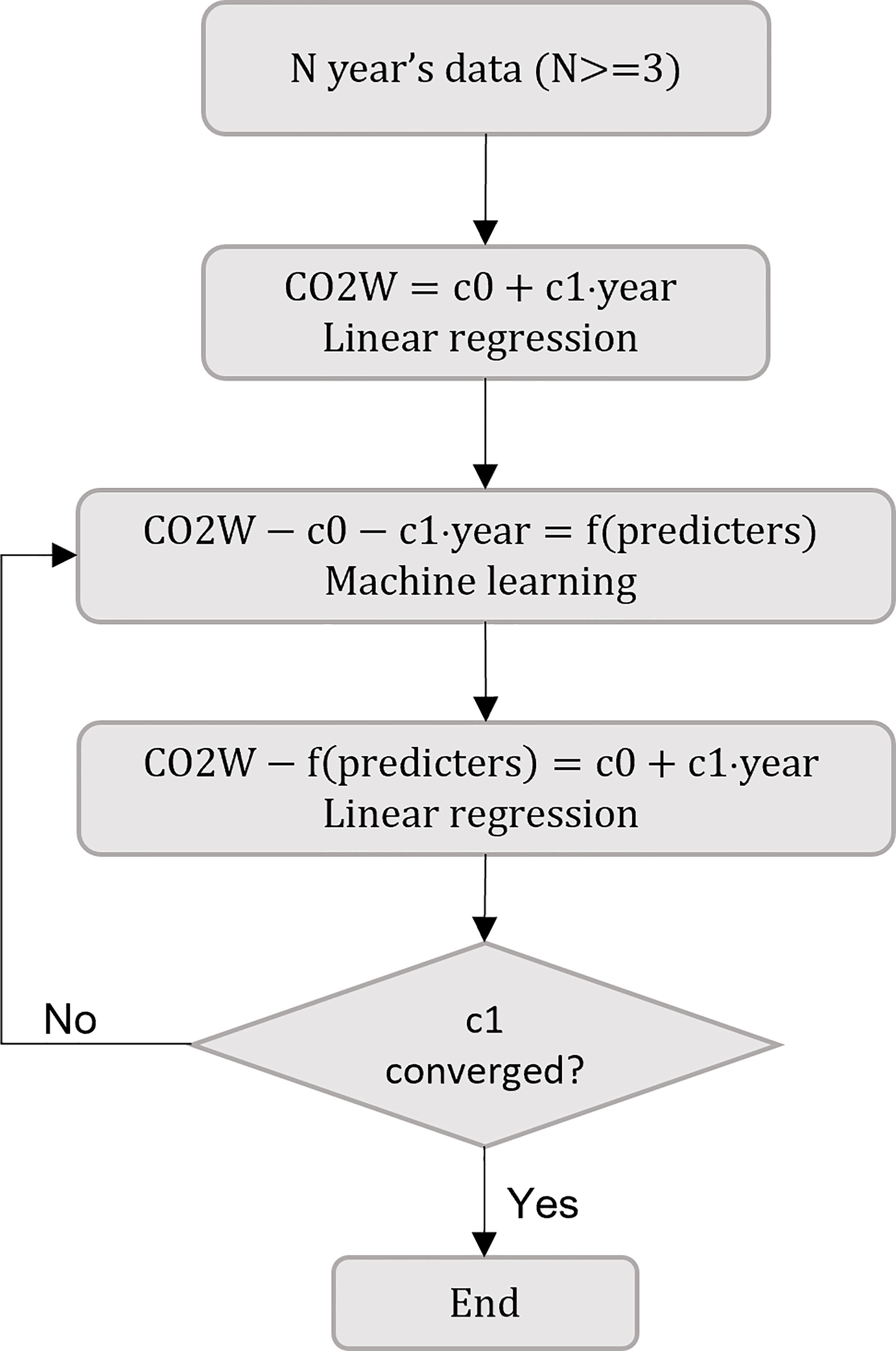
Figure 1 Flow chart of the iteration method for trend extraction.
where T1 and T2 are time parameter in year. For training machine learning models, the atmospheric CO2 trends obtained by Eq.(2) were used to normalize the observed CO2 values to the reference year 2000 by the equation:
where ± is positive when i<2000 and negative when i>2000. At i=2000, the trend correction is zero. Global CO2 concentrations were constructed by adding or subtracting the trend correction of Eq.(3) to the predicted CO2 values. The process is the inverse of the normalization. Using atmospheric CO2 trends for data normalization avoided problems in using oceanic CO2 trends directly, e.g., insufficient data points in the early and later years and the difficulty of determining the best data length for trend extraction.
Models
We deployed three machine learning models: Random Forest (RF), Gradient Boost Machine (GBM), and Feedforward Neural Network (FNN). Using multiple models has the merit of mutual overfit checking and compensating model weakness with each other.
RF was proved to be a robust method for modelling carbon flux at the global scale (Zeng et al., 2020) and was applied to global ocean CO2 mapping recently (Gregor et al., 2019). RF partitions a training dataset into subsets repeatedly by random sampling and uses the subsets to construct trees. We used the python library of Ranger (Wright and Ziegler, 2017) which implements the regression algorithm using a two-stage randomization procedure to partition trees. Given a subset, the root node in a tree is recursively split into binary nodes until the number of data points in the leaf nodes becomes no larger than a specified number. In each split, the RF randomly selects a subset of predictor variables and searches them for splitting points that minimize node impurity (Ishwaran, 2015). In making a prediction, a set of predictors are passed through branches of nodes according to the splitting rule until the journey ends up in a leaf node. The mean of the target variable in the leaf node is taken as an estimate. Then the mean estimate of all leaf nodes is used as the prediction. Sensitive configuration factors for the RF include the number of trees and the number of data points in the leaf nodes (Zeng et al., 2020). The default setting includes 500 trees and 5 data points. We raised the data points to 100 based on our experiments with the ocean CO2 data discussed in the data section to prevent hot spots in predicted CO2 in the southern oceans where vast empty areas exist in certain months. The configuration yielded good validation results.
A decision-tree-based GBM emerged in the ocean CO2 mapping recently (Gregor et al., 2019; Gregor and Gruber, 2021). Like a RF, a GBM combines weak learners into a single strong learner (Natekin and Knoll, 2013), but in an iterative fashion. It adds trees one at a time, and existing trees are not changed. We used the python library of LightGBM (Ke et al., 2017). Instead of the level-wise strategy of the RF, the GBM grows a tree leaf-wise by splitting nodes that produce the highest loss change until the number of leaf nodes becomes no larger than a specified number. The observed values of the target variable are assigned to the leaf nodes of the first tree. Then, the residuals of the previous predictions minus observations are assigned to the leaf nodes of a subsequent tree. A gradient descent procedure is used to obtain parameters that improve the accuracy of predictions. By experimenting with our ocean CO2 data and using the RF as a reference, we found that LightGBM performed well with 500 trees and a maximum number of 100 terminal nodes in a tree.
FNN has been used for ocean CO2 mapping since the early 2010s (e.g., Landschützer et al., 2013; Zeng et al., 2014). FNN has a layered structure, including an input layer, one or more hidden layers, and an output layer. Neurons between adjacent layers are fully connected. A neuron in the hidden layer uses an activation function to transform the weighted sum of inputs to form an input for the neuron in the output layer, which in turn transforms the weighted sum of inputs to form a prediction. Details of the FNN method can be found in Svozil et al. (1997) and abundant other references. We used python’s MLPRegressor model with one hidden layer and 64 hidden neurons, which is the same as that used by Zeng et al. (2014). Their investigations show that the setting yielded uncertainties in the level of grid mean variation of measurements. We raised the default maximum training iterations of MLPRegressor from 200 to 500. Our tests indicate that when the iterations were larger than 300, doubling or tripling the number did not make a substantial change in the flux estimate. Training the FNN took a much longer time than training the RF and GBM. As the trend extraction and validation discussed later involve many rounds of training, we had to set a fixed number of training iterations so that the training could be completed within a reasonable amount of time. The settings also yielded results well harmonized with those of the RF and GBM.
We validated the model performance by a leave-one-year-out (LOYO) method. Given N years of data, N validations were done by setting aside one year’s data for validation and using the remaining N-1 years of data for training. A model’s performance was evaluated by the mean bias. The validation method has an advantage over the conventional n-fold method in that the validation data of LOYO are more likely to come from unsampled domains of the training data. Another advantage is that LOYO can also be used to detect trends. If the target variable has an increasing trend, a model trained with data in early years tends to make predictions smaller than the observations in later years and vice versa.
Data
We extracted monthly CO2 fugacity (fCO2) in 1×1-degree grids from the track-gridded database of SOCAT version 2021 (Sabine et al., 2013; Pfeil et al., 2013; Bakker et al., 2016). We relaxed the criteria of Zeng et al. (2014) to include data when fCO2 values are between 50 μatm and 1000 μatm and salinity is larger than 15 g kg-1. A total of 273,456 data points were extracted for 1980-2020. We confined the fCO2 training data set to post-1980 due to large uncertainties in the early measuring techniques (Sasse et al., 2013). The sources of predictor variables are shown in Table 1. The monthly climatology of MODIS-AQUA and MODIS-TERRA of 2002-2019 in 0.083×0.083-degree grids (Hu et al., 2012.) were combined and re-binned into 1x1-degree grids. The values of CHL and MDL were scaled by log(1+CHL) and log(1+MDL) to reduce the skewness of sample distribution. Filling missing CHL data in high latitudes with a small constant is a common practice (Gregor and Gruber, 2021; Chau et al., 2022). We filled the missing CHL in a grid with the smallest observed value in that grid. The data of SST (Ishii et al., 2005) and SSS (Zweng et al., 2019) were used without pre-processing. For flux calculation, we used the wind speed (WIND) and surface pressure (Ps) of the fifth generation ECMWF atmospheric reanalysis of the global climate (ERA5) (Hersbach et al., 2020), and the mole fraction of air CO2 (xCO2A) of NOAA’s Marine Boundary Layer Reference (Conway et al., 1994; Dlugokencky et al., 2021). The monthly WIND and Ps in 0.25×0.25 degrees were averaged to 1×1 degree. The surface xCO2A in sine latitude grids was interpolated to 1×1 degree.
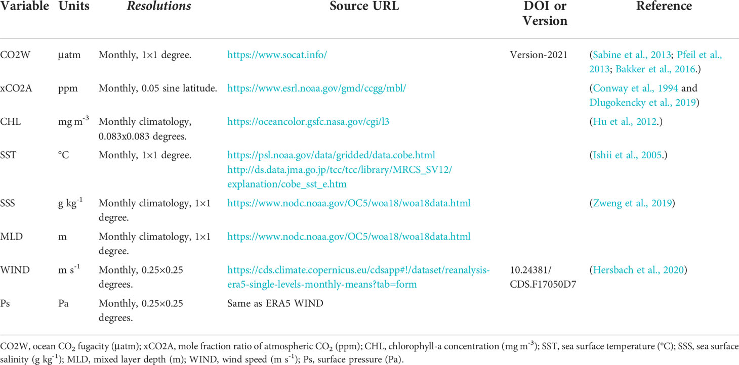
Table 1 Data sources.
Comparison
We compared our estimates with seven machine learning products included in GCB-2021 (Table 2). We recalculated their fluxes by the same procedure to eliminate the effect of using different flux dependent data and coefficients. As each product has a different spatial coverage, we adjusted their annual fluxes using the equation

Table 2 Datasets for comparison.
where FML3 (PgC a-1) is the mean annual flux of NIES-ML3 (the ensemble mean of the three models) in the available period of a pair of products under comparison and F’ML3 (PgC a-1) is the mean annual flux of NIES-ML3 in the grids where both products have data. The adjustment was intended to bring fluxes with different spatial coverages to the same coverage as the NIES-ML3.
Results and discussion
CO2 trend
The ocean CO2 trends obtained using the iteration method in Figure 1 with the longest available data are shown in Figure 2A along with the annual increase rates of global atmospheric CO2 concentrations (ppm) (Friedlingstein et al., 2022). Because of data scarcity, the extracted trends fluctuate dramatically when the data length is short and converge gradually (Figure 2B). Sutton et al. (2019) pointed out that the number of years of observations needed (YON) to detect a statistically significant trend over variability ranges from 8 to 15 years at several open ocean sites. It is reasonable to assume the same YON range for open oceans. Ideally, the trend for a year should be extracted with the shortest data length possible. As it is difficult to determine the smallest stabilization length and the trend does not change much after 10 to 15 years, we presented the trend with the maximum data length. The extracted trends appear to track the decadal trends of the atmospheric CO2 in 1990-2015 obtained by Eq.(2) with T1 = 20 year and T2 = 40 year.
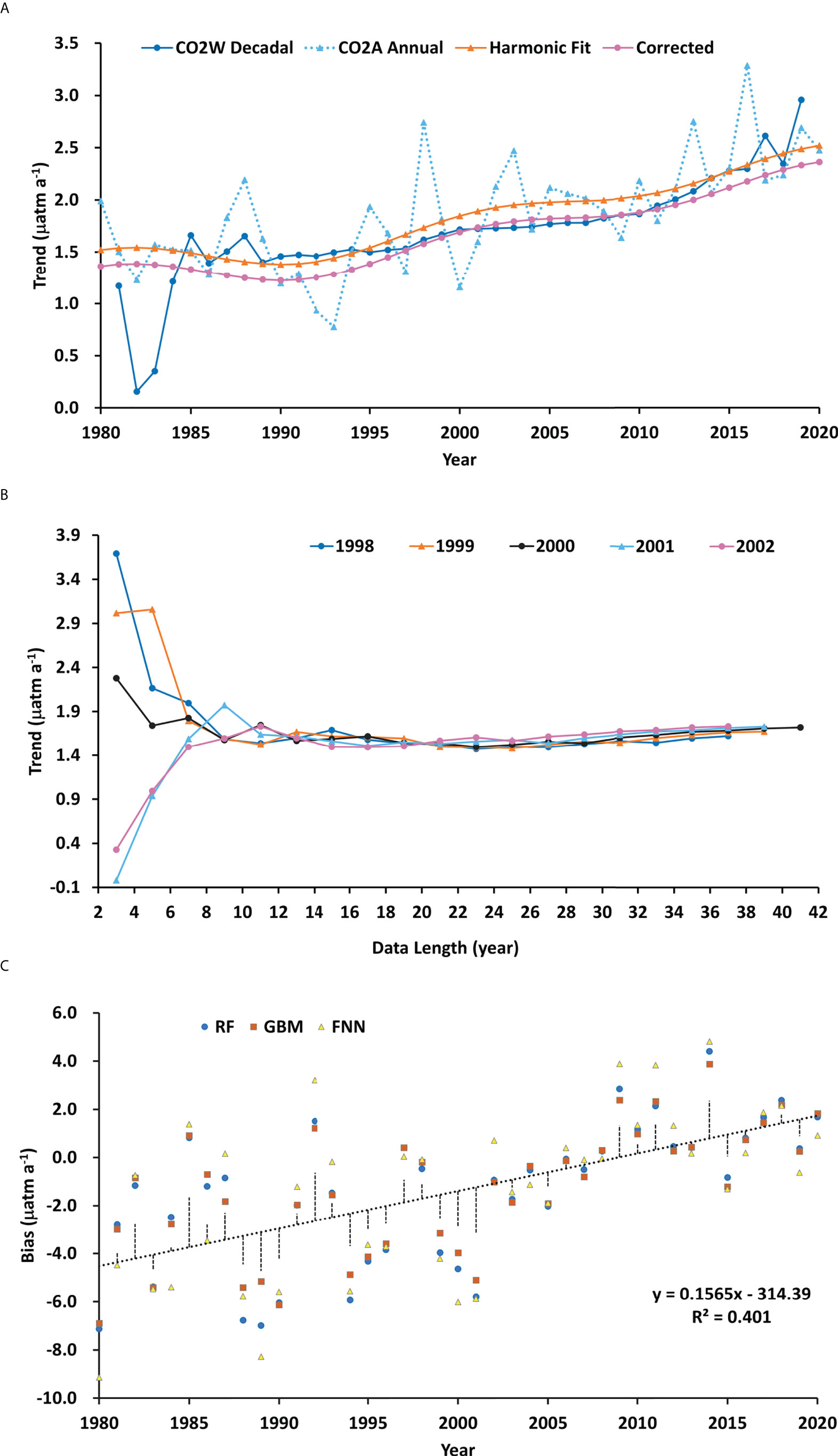
Figure 2 Trends extraction. (A) The trend of ocean CO2 for a target year (blue) was estimated by using the iteration method with the longest data length around the year. The final trends to be used for data normalization (magenta) are the corrected function fitting trends (orange) of the annual increase rate of air CO2 (cyan). (B) Examples of trend variations with data length for the target years 1998-2002. (C) The trend of CO2 biases (prediction – observation) detected by LOYO with CO2 data normalized by the uncorrected decadal trends of air CO2. The vertical lines show the standard residuals of the regression.
We applied the LOYO method to the data normalized by the trends of Eq.(2). A small trend of 0.1565 μatm a-1 exists in the residual of model prediction minus observations (Figure 2C). The p-value of the trend is 9×10⁻⁶, indicating that the trend is significant. We subtracted the residual trend from the decadal air CO2 trends and yielded the trends shown in magenta line in Figure 2A. The numerical values of the corrected trends are listed in Table 3. They were used for final data normalization. The corrected trends agree well with the extracted ocean CO2 trends in 1996-2013, during which the data length used to extract ocean CO2 trends is longer than the YON of Sutton et al. (2019). The corrected trends in early 2000s are close to the those obtained by Sutton et al. (2019) for the time series station WHOTS in the subtropical North Pacific and Stratus in the South Pacific gyre in 2004-2013. Although the corrected trends before 1997 are smaller than those used by Takahashi et al. (2009) and Zeng et al.,(2014) for data normalization, they are within the range of trends summarized by Takahashi et al. (2009).
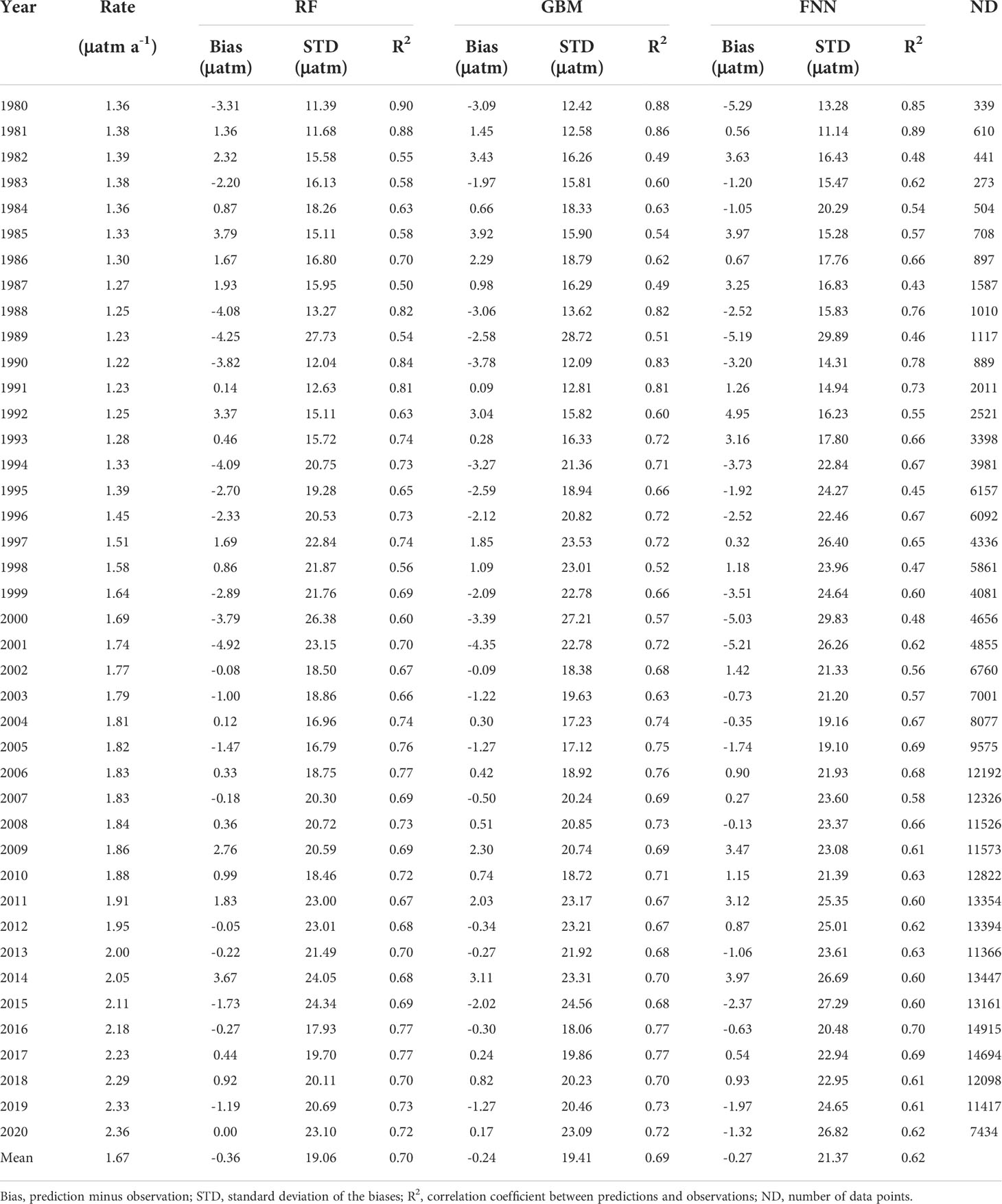
Table 3 Trends for data normalization and LOYO validation results.
Validation and uncertainty
The performances of the three models were evaluated by the LOYO method with the normalized CO2. The validation yields small biases (prediction minus observation) and good correlation coefficients. The annual mean bias ranges between -4.82 and 3.79 μatm for RF, between -4.34 and 3.92 μatm for GBM, and between -5.29 and 4.95 μatm for FNN (Table 3). Their mean biases are -0.36 μatm, -0.24 μatm, and -0.27 μatm, respectively. The correlation coefficient R2 in individual years ranges between 0.50 and 0.90 for RF, between 0.49 and 0.88 for GBM, and between 0.43 and 0.89 for FNN. Their mean R2 are 0.70, 0.69, and 0.62, respectively. Figure 3 shows the goodness of fit of the three models. The bias and R2 in the figure were calculated directly using all validation data points and therefore are equivalent to the weighted mean bias and R2 in Table 3.
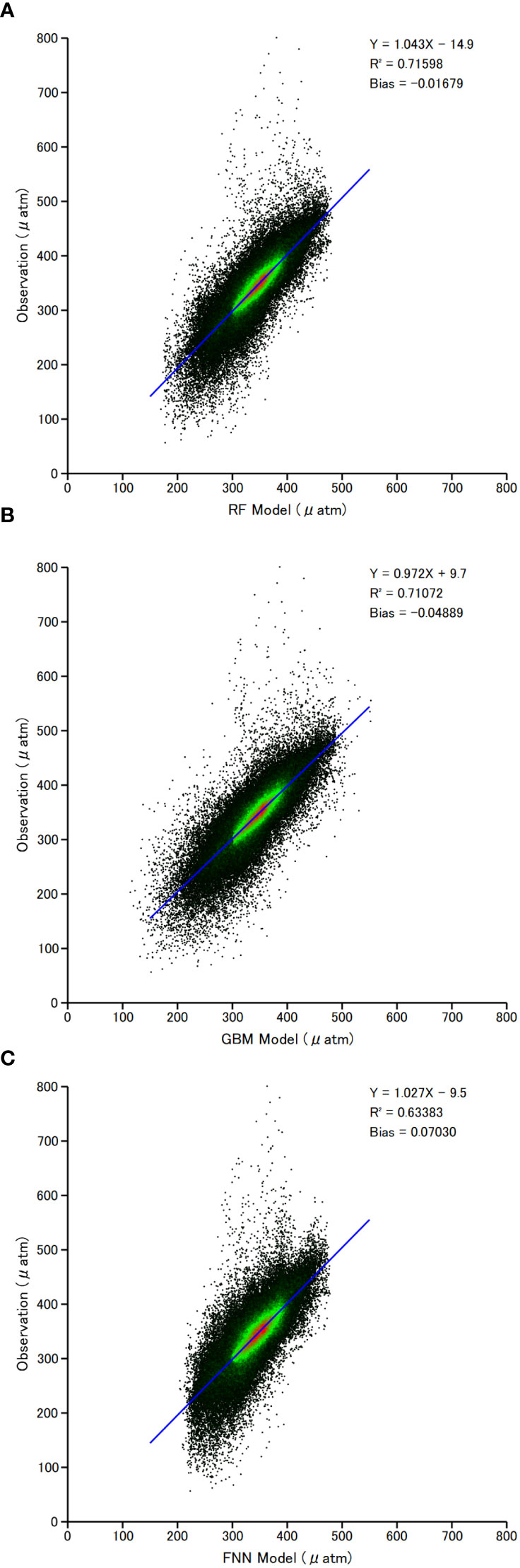
Figure 3 Model predictions vs observations of ocean CO2 fugacity using normalized data with the trends in Table 3. Predictions come from 41 validations for each target year between 1980 and 2020. The colour indicates the density of data points. (A) Results of the RF model. (B) Results of the GBM model. (C) Results of the FNN model.
At the CO2 level in year 2000, one unit CO2 change results in a flux change of 0.19 PgC a-1. We calculated the flux uncertainties approximately by multiplying this value with the biases in Table 3. For the RF model, the uncertainty ranges from -0.93 PgC a-1 to 0.72 PgC a-1 and the mean is -0.07 PgC a-1. The GBM model has a smaller uncertainty range from -0.83 PgC a-1 to 0.74 PgC a-1 and a mean of -0.05 PgC a-1. The FNN model has the largest uncertainty range from -1.01 PgC a-1 to 0.94 PgC a-1 and a mean of -0.05 PgC a-1.
Comparison
The fluxes of the products in Table 2 were recalculated by equations in the Appendix and adjusted by Eq.(4) for comparison. The offset added to the products is 0.00 μatm for NIES-NN and JENA, 0.22 μatm for JMA-MLR, 0.01 μatm for MPI-SOMFFN, 0.34 μatm for CMEMS-FFNN, 0.07 μatm for CSIR-ML6, and 0.01 μatm for OceanSODA-ETHZ.
The difference between NIES-ML3 and NIES-NN is small in 1991-2006 but much larger in the early and late years (Figure 4A). NIES-NN used a constant trend of 1.54 μatm a-1 to normalize data to the reference year 2000. The trend is larger than those in Table 3 before 1998 and smaller after that year. This resulted in larger reconstructed CO2 in the periods. The bias caused larger flux estimates in the years further away from the reference year. In 1985 and 2019, NIES-NN flux is larger than that of NIES-ML3 by 0.536 PgC a-1 and 1.057 PgC a-1 respectively. The latter is close to half of the fluxes in recent years. Near the reference year of 2000, NIES-NN is smaller than NIES-ML3 in the order of 0.1 PgC a-1. The JMA-MLR product (Iida et al., 2021) also shows an arch-shaped flux trend like NIES-NN does. Again, the differences are larger in the early and late years of the comparison period, especially in the 1990s. This is expected as the regression method of JMA-MLR includes a linear term of time for each geographic box, which is equivalent to using a constant trend for data normalization. The flux estimate of JMA-MLR is larger than that of NIES-ML in all years. In 1990 to 2020, JMA-MLR flux is larger than that of NIES-ML3 by 0.699 PgC a-1 and 0.506 PgC a-1 respectively. They are about a quarter of the flux in recent years.
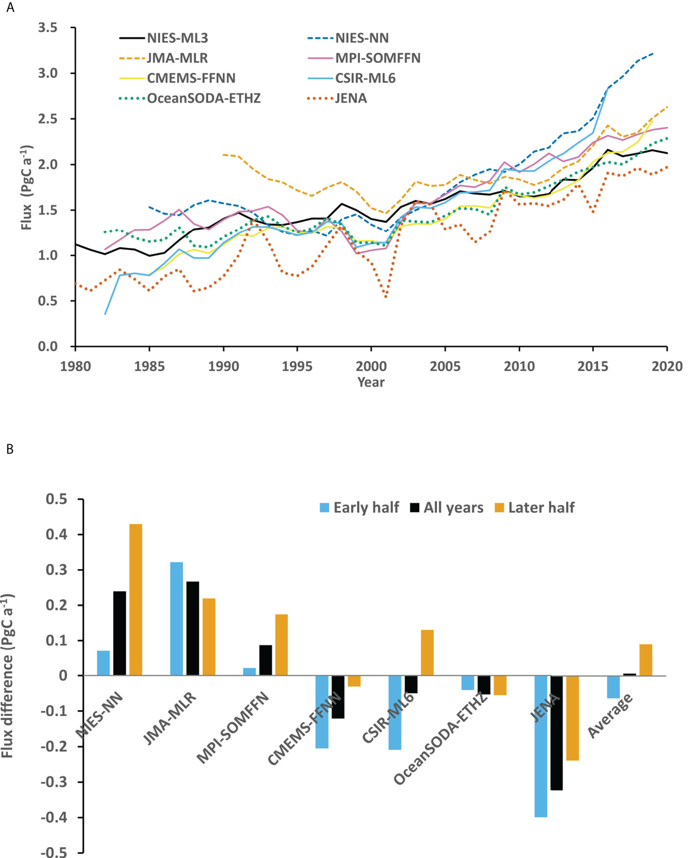
Figure 4 Comparisons with machine learning products included in GSB-2021. Fluxes were recalculated by the same method and adjusted to have the same spatial coverage of NIES-ML3. (A) Variations of annual fluxes with time. (B) Mean differences of third-party products minus NIES-ML3 in the whole available period, the early half years, and later half years.
Instead of using explicit trends to normalize data or including a linear term of time in the regression, MPI-SOMFFN (Landschützer et al., 2016), CMEMS-FFNN (Chau et al., 2022), CSIR-ML6 (Gregor et al., 2019), and OceanSODA-ETHZ (Gregor and Gruber, 2021) used atmospheric CO2 as a predictor so that their models could learn the trends implicitly. Their flux trend patterns indicate different implicit CO2 trends. While the fluxes of MPI-SOMFFN and OceanSODA-ETHZ remain rather flat before 2000 and then increase with time, the fluxes of CMEMS-FFNN and CSIR-ML6 show a trend before the early 1990s and after 2000 and remain at a similar level in between. The JENA method (Rödenbeck et al., 2013) involves an inversion model for the ocean chemistry coupled with the atmospheric CO2 of an atmospheric transport model. It has the largest inter-annual flux variations. Note that all products except for JENA are monthly with a 1×1-degree spatial resolution. We calculated the monthly mean CO2 of JENA in 2×2.5-degree grids using its daily dataset and then filled the 1x1-degree grids with values in the nearest source grids. A different averaging and re-gridding method may yield a different result. The day of the year is also a predictor of CSIR-ML6.
Figure 4B reveals several patterns in the flux differences between NIES-ML3 and other products. The black, cyan, and orange bars represent the mean of a product minus NIES-ML3 in the whole available period, in the early half, and the latter-half years, respectively. NIES-ML3 agrees with CSIR-ML6 and OceanSODA-ETHZ the most in terms of the overall mean difference, which is -0.050 PgC a-1 and -0.053 PgC a-1, respectively. Their p-values of two tailed t-test with a significance level of 95%, 0.615 and 0.478 respectively, indicate that the differences are insignificant. While the flux of CSIR-ML6 is smaller than that of NIES-ML3 in the early-half years and larger in the latter-half years, the long-term change of NIES-ML3 is more consistent with that of OceanSODA-ETHZ. The differences between NIES-ML3 and MPI-SOMFFN (0.088 PgC a-1, p-value=0.304), and between NIES-ML3 and CMEMS-FFNN (-0.121 PgC a-1, p-value=0.151) are moderate but insignificant. The fluxes of NIES-NN and JMA-MLR are much larger than that of NIES-ML3, by 0.240 PgC a-1 (p-value=0.030) and 0.267 PgC a-1 (p-value=0.000) respectively, especially in the latter-half years of NIES-NN and the early-half years of JMA-MLR. The largest difference was between JENA and NIES-ML3 (-0.322 PgC a-1, p-value=0.000). Overall, the difference between NIES-ML3 and other products is small, about 0.007 PgC a-1.
Conclusion
Our results point out that the ocean CO2 trends are an important factor affecting the global ocean CO2 reconstruction and flux estimate by machine learning methods. So far, explicit trend methods assumed a constant trend. They yielded much larger flux estimates than most implicit methods in the early and later years of the modelled period. Because the ocean CO2 trends tend to track the trends of air CO2 and the later increased with time, using a constant ocean CO2 trend tends to underestimate the concentration in those years. We proposed a new method to use variant trends for an explicit method that applies machine learning to trend removed data. On average, our flux estimates are significantly lower those of NIES-NN and JMA-MLR. Comparing to the implicit methods, they are smaller than that of MPI-SOMFFN but larger than those of CSIR-ML6, OceanSODA-ETHZ and CMEMS-FFNN. Even though the differences of implicit methods are less significant than those of the explicit methods, the fluxes among the implicit methods depart substantially in early and recent years. This reveals that the ocean CO2 trends obtained by the implicit methods could be largely different. All the implicit methods regrouped data by clustering. While the merit point of clustering to regroup data by their biogeochemical properties have been stressed, its demerit point of worsening the data scarcity problem was rarely discussed. Therefore, our results are expected not only to enhance the accuracy of flux estimate by machine learning but also to provide a reference to investigate the trend differences of the implicit methods.
Data availability statement
The modelled results can be obtained from https://www.nies.go.jp/doi/10.17595/20220311.001-e.html. Other data and code used in the study may be provided upon request. Further inquiries can be directed to the corresponding author.
Author contributions
JZ: Model experiment design, data processing, and draft manuscript. YI: Flux comparisons. TM: Advice on satellite data. TS: Result checking and advice on carbon budget issues. All authors contributed to the article and approved the submitted version.
Acknowledgments
This study was partly supported by NIES GOSAT and GOSAT-2 projects. The Surface Ocean CO2 Atlas (SOCAT) is an international effort, endorsed by the International Ocean Carbon Coordination Project (IOCCP), the Surface Ocean Lower Atmosphere Study (SOLAS), and the Integrated Marine Biosphere Research (IMBeR) program, to deliver a uniformly quality-controlled surface ocean CO2 database. We thank the many researchers and funding agencies responsible for the collection of data and quality control for their contributions to SOCAT.
Conflict of interest
The authors declare that the research was conducted in the absence of any commercial or financial relationships that could be construed as a potential conflict of interest.
Publisher’s note
All claims expressed in this article are solely those of the authors and do not necessarily represent those of their affiliated organizations, or those of the publisher, the editors and the reviewers. Any product that may be evaluated in this article, or claim that may be made by its manufacturer, is not guaranteed or endorsed by the publisher.
References
Bakker D. C. E., Pfeil B., Landa C. S., Metzl N., O’Brien K. M., Olsen A., et al. (2016). A multi-decade record of high-quality CO2 data in version 3 of the surface ocean CO2 atlas (SOCAT). Earth Syst. Sci. Data 8, 383–413. doi: 10.5194/essd-8-383-2016
Bates N., Astor Y., Church M., Currie K., Dore J., Gonaález-Dávila M., et al. (2014). A time-series view of changing ocean chemistry due to ocean uptake of anthropogenic CO2 and ocean acidification. oceanog 27, 126–141. doi: 10.5670/oceanog.2014.16
Chau T. T. T., Gehlen M., Chevallier F. (2022). A seamless ensemble-based reconstruction of surface ocean <i<p</i<CO<sub<2</sub< and air–sea CO<sub<2</sub< fluxes over the global coastal and open oceans. Biogeosciences 19, 1087–1109. doi: 10.5194/bg-19-1087-2022
Conway T. J., Tans P. P., Waterman L. S., Thoning K. W., Kitzis D. R., Masarie K. A., et al. (1994). Evidence for interannual variability of the carbon cycle from the national oceanic and atmospheric Administration/Climate monitoring and diagnostics laboratory global air sampling network. J. Geophys. Res. 99, 22831. doi: 10.1029/94JD01951
Denvil-Sommer A., Gehlen M., Vrac M., Mejia C. (2019). LSCE-FFNN-v1: a two-step neural network model for the reconstruction of surface ocean CO2 over the global ocean. Geosci. Model. Dev. 12, 2091–2105. doi: 10.5194/gmd-12-2091-2019
Dickson A. G., Sabine C. L., Christian J. R. (2007). Guide to best practices for ocean CO2 measurements. (Sidney, Canada: PICES Special Publication 3, North Pacific Marine Science Organization) 196 pp. 3, IOCCP Report No. 8.
Dlugokencky E. J., Thoning K. W., Lang P. M., Tans P. P. (2021). NOAA Greenhouse gas reference from atmospheric carbon dioxide dry air mole fractions from the NOAA ESRL carbon cycle cooperative global air sampling network.
Fay A. R., Gregor L., Landschützer P., McKinley G. A., Gruber N., Gehlen M., et al. (2021). SeaFlux: harmonization of air–sea CO2 fluxes from surface pCO2 data products using a standardized approach. Earth Syst. Sci. Data 13, 4693–4710. doi: 10.5194/essd-13-4693-2021
Fay A. R., McKinley G. A. (2013). Global trends in surface ocean pCO2 from in situ data: GLOBAL TRENDS IN SURFACE OCEAN pCO2. Global Biogeochem. Cycles 27, 541–557. doi: 10.1002/gbc.20051
Friedlingstein P., Jones M. W., O’Sullivan M., Andrew R. M., Bakker D. C. E., Hauck J., et al. (2022). Global carbon budget 2021. Earth Syst. Sci. Data 14, 1917–2005. doi: 10.5194/essd-14-1917-2022
Gloege L., McKinley G. A., Landschützer P., Fay A. R., Frölicher T. L., Fyfe J. C., et al. (2021). Quantifying errors in observationally based estimates of ocean carbon sink variability. Global Biogeochem Cycles 35, 1–14. doi: 10.1029/2020GB006788
Gregor L., Gruber N. (2021). OceanSODA-ETHZ: a global gridded data set of the surface ocean carbonate system for seasonal to decadal studies of ocean acidification. Earth Syst. Sci. Data 13, 777–808. doi: 10.5194/essd-13-777-2021
Gregor L., Lebehot A. D., Kok S., Scheel Monteiro P. M. (2019). A comparative assessment of the uncertainties of global surface ocean CO2 estimates using a machine-learning ensemble (CSIR-ML6 version 2019a) – have we hit the wall? Geosci. Model. Dev. 12, 5113–5136. doi: 10.5194/gmd-12-5113-2019
Hersbach H., Bell B., Berrisford P., Hirahara S., Horányi A., Muñoz-Sabater J., et al. (2020). The ERA5 global reanalysis. Q.J.R. Meteorol. Soc 146, 1999–2049. doi: 10.1002/qj.3803
Hu C., Lee Z., Franz B. (2012). Chlorophyll-a algorithms for oligotrophic oceans: A novel approach based on three-band reflectance difference: A NOVEL OCEAN CHLOROPHYLL a ALGORITHM. J. Geophys. Res. 117:1–25. doi: 10.1029/2011JC007395
Iida Y., Kojima A., Takatani Y., Nakano T., Sugimoto H., Midorikawa T., et al. (2015). Trends in pCO2 and sea–air CO2 flux over the global open oceans for the last two decades. J. Oceanogr 71, 637–661. doi: 10.1007/s10872-015-0306-4
Iida Y., Takatani Y., Kojima A., Ishii M. (2021). Global trends of ocean CO2 sink and ocean acidification: an observation-based reconstruction of surface ocean inorganic carbon variables. J. Oceanogr 77, 323–358. doi: 10.1007/s10872-020-00571-5
Ishii M., Shouji A., Sugimoto S., Matsumoto T. (2005). Objective analyses of sea-surface temperature and marine meteorological variables for the 20th century using ICOADS and the Kobe collection. Int. J. Climatol 25, 865–879. doi: 10.1002/joc.1169
Ishwaran H. (2015). The effect of splitting on random forests. Mach. Learn 99, 75–118. doi: 10.1007/s10994-014-5451-2
Jones S. D., Le Quéré C., Rödenbeck C., Manning A. C., Olsen A. (2015). A statistical gap-filling method to interpolate global monthly surface ocean carbon dioxide data: STATISTICAL INTERPOLATION OF OCEAN CO2. J. Adv. Model. Earth Syst. 7, 1554–1575. doi: 10.1002/2014MS000416
Ke G., Meng Q., Finley T., Wang T., Chen W., Ma W., et al. (2017). LightGBM: A highly efficient gradient boosting decision tree 9. Adv. Neural Inf. Process. Syst. 30, 1–9.
Khatiwala S., Tanhua T., Mikaloff Fletcher S., Gerber M., Doney S. C., Graven H. D., et al. (2013). Global ocean storage of anthropogenic carbon. Biogeosciences 10, 2169–2191. doi: 10.5194/bg-10-2169-2013
Landschützer P., Gruber N., Bakker D. C. E. (2016). Decadal variations and trends of the global ocean carbon sink: DECADAL AIR-SEA CO2 FLUX VARIABILITY. Global Biogeochem. Cycles 30, 1396–1417. doi: 10.1002/2015GB005359
Landschützer P., Gruber N., Bakker D. C. E., Schuster U., Nakaoka S., Payne M. R., et al. (2013). A neural network-based estimate of the seasonal to inter-annual variability of the Atlantic ocean carbon sink. Biogeosciences 10, 7793–7815. doi: 10.5194/bg-10-7793-2013
Laruelle G. G., Landschützer P., Gruber N., Tison J.-L., Delille B., Regnier P. (2017). Global high-resolution monthly pCO2 climatology for the coastal ocean derived from neural network interpolation. Biogeosciences 14, 4545–4561. doi: 10.5194/bg-14-4545-2017
McKinley G. A., Fay A. R., Takahashi T., Metzl N. (2011). Convergence of atmospheric and north Atlantic carbon dioxide trends on multidecadal timescales. Nat. Geosci 4, 606–610. doi: 10.1038/ngeo1193
McKinley G. A., Pilcher D. J., Fay A. R., Lindsay K., Long M. C. (2016). Lovenduski, N.S.: Timescales for detection of trends in the ocean carbon sink. Nature 530, 469–472. doi: 10.1038/nature16958
Nakaoka S., Telszewski M., Nojiri Y., Yasunaka S., Miyazaki C., Mukai H., et al. (2013). Estimating temporal and spatial variation of ocean surface pCO2 in the north pacific using a self-organizing map neural network technique. Biogeosciences 10, 6093–6106. doi: 10.5194/bg-10-6093-2013
Natekin A., Knoll A. (2013). Gradient boosting machines, a tutorial. Front. Neurorobot 7. doi: 10.3389/fnbot.2013.00021
Pfeil B., Olsen A., Bakker D. C. E., Hankin S., Koyuk H., Kozyr A., et al. (2013). A uniform, quality controlled surface ocean CO2 atlas (SOCAT). Earth Syst. Sci. Data 5, 125–143. doi: 10.5194/essd-5-125-2013
Rödenbeck C., Keeling R. F., Bakker D. C. E., Metzl N., Olsen A., Sabine C., et al. (2013). Global surface-ocean pCO2 and sea–air CO2 flux variability from an observation-driven ocean mixed-layer scheme. Ocean Sci. 9, 193–216. doi: 10.5194/os-9-193-2013
Sabine C. L. (2004). The oceanic sink for anthropogenic CO2. Science 305, 367–371. doi: 10.1126/science.1097403
Sabine C. L., Hankin S., Koyuk H., Bakker D. C. E., Pfeil B., Olsen A., et al. (2013). Surface ocean CO2 atlas (SOCAT) gridded data products. Earth Syst. Sci. Data 5, 145–153. doi: 10.5194/essd-5-145-2013
Sasse T. P., McNeil B. I., Abramowitz G. (2013a). A novel method for diagnosing seasonal to inter-annual surface ocean carbon dynamics from bottle data using neural networks (preprint). Biogeochem.: Open Ocean 10:4319–4340. doi: 10.5194/bgd-9-15329-2012
Sasse T. P., McNeil B. I., Abramowitz G. (2013b). A new constraint on global air-sea CO2 fluxes using bottle carbon data: DATA-BASED CONTEMPORARY CO2 UPTAKE. Geophys. Res. Lett. 40, 1594–1599. doi: 10.1002/grl.50342
Sutton A. J., Feely R. A., Maenner-Jones S., Musielwicz S., Osborne J., Dietrich C., et al. (2019). Autonomous seawater pCO2 and pH time series from 40 surface buoys and the emergence of anthropogenic trends. Earth Syst. Sci. Data 11, 421–439. doi: 10.5194/essd-11-421-2019
Svozil D., Kvasnicka V., Pospichal J. (1997). Introduction to multi-layer feed-forward neural networks. Chemometrics Intelligent Lab. Syst., 43–62 39. doi: 10.1016/S0169-7439(97)00061-0
Takahashi T., Sutherland S. C., Wanninkhof R., Sweeney C., Feely R. A., Chipman D. W., et al. (2009). Climatological mean and decadal change in surface ocean pCO2, and net sea–air CO2 flux over the global oceans. Deep Sea Res. Part II: Topical Stud. Oceanogr. 56, 554–577. doi: 10.1016/j.dsr2.2008.12.009
Wanninkhof R. (2014). Relationship between wind speed and gas exchange over the ocean revisited: Gas exchange and wind speed over the ocean. Limnol. Oceanogr. Methods 12, 351–362. doi: 10.4319/lom.2014.12.351
Watson A. J., Schuster U., Shutler J. D., Holding T., Ashton I. G. C., Landschützer P., et al. (2020). Revised estimates of ocean-atmosphere CO2 flux are consistent with ocean carbon inventory. Nat. Commun. 11, 4422. doi: 10.1038/s41467-020-18203-3
Weiss R. F. (1974). Carbon dioxide in water and seawater: the solubility of a non-ideal gas. Mar. Chem. 2, 203–215. doi: 10.1016/0304-4203(74)90015-2
Weiss R. F., Price B. A. (1980). Nitrous oxide solubility in water and seawater. Mar. Chem. 8, 347–359. doi: 10.1016/0304-4203(80)90024-9
Wright M.N, Ziegler A. (2017). ranger : A Fast Implementation of Random Forests for High Dimensional Data in C++ and R. J. Stat. Soft 77. doi: 10.18637/jss.v077.i01
Zeng J., Matsunaga T., Tan Z.-H., Saigusa N., Shirai T., Tang Y., et al. (2020). Global terrestrial carbon fluxes of 1999–2019 estimated by upscaling eddy covariance data with a random forest. Sci. Data 7, 313. doi: 10.1038/s41597-020-00653-5
Zeng J., Nojiri Y., Landschützer P., Telszewski M., Nakaoka S. (2014). A global surface ocean fCO2 climatology based on a feed-forward neural network. J. Atmospheric Oceanic Technol. 31, 1838–1849. doi: 10.1175/JTECH-D-13-00137.1
Zweng M. M., Reagan J. R., Seidov D., Boyer T. P., Locarnini R. A., Garcia H. E., et al. (2019). World ocean atlas 2018, volume 2: Salinity Vol. 82. Ed. Mishonov A. (Silver Spring, MD, USA: U.S. DEPARTMENT OF COMMERCE National Oceanic and Atmospheric Administration National Environmental Satellite, Data, and Information Service National Centers for Environmental Information.), 50.
Appendix
According to Wanninkhof (2014), air-sea CO2 fluxes can be calculated by the partial pressures of CO2 in the air (pCO2A, μatm) and seawater (pCO2W, μatm):
where k0 (mol L-1 atm-1) denotes the solubility of CO2 in seawater. It is a function of seawater temperature (K) and salinity (g kg-3):
The gas transfer velocity kw (cm h-1) is a function of wind speed WIND (m s-1) 10 m above the surface and the dimensionless Schmidt number:
in which α is a coefficient and the unit of SST is Celsius. Wanninkhof (2014) obtained α as 0.251 (cm h-1) (m s-1)-2 using the high-resolution data of Cross-Calibrated Multi-Platform wind vector analysis (CCMP). The study of Fay et al. (2021) shows that α should take a larger value when a monthly wind with 1×1-degree resolution is used. We adopted their value of 0.271 (cm h-1) (m s-1)-2 for ERA5 wind.
The predicted fCO2 (μatm) was converted to partial pressure (μatm) by the method of Weiss (1974) and Dickson et al. (2007):
in which the unit of SST is Kelvin. The partial pressure of air CO2 was calculated from xCO2A by:
The vapor pressure of seawater pH2O (atm) was calculated by the method of Weiss & Price (1980):
with SST in Kelvin.
Keywords: global ocean CO2 flux, machine learning, random forest, gradient boost machine, neural network
Citation: Zeng J, Iida Y, Matsunaga T and Shirai T (2022) Surface ocean CO2 concentration and air-sea flux estimate by machine learning with modelled variable trends. Front. Mar. Sci. 9:989233. doi: 10.3389/fmars.2022.989233
Received: 08 July 2022; Accepted: 24 August 2022;
Published: 14 September 2022.
Edited by:
Laurent Coppola, UMR7093 Laboratoire d’océanographie de Villefranche (LOV), FranceReviewed by:
Thibaut Wagener, Aix-Marseille Université, FranceCathy Wimart-Rousseau, GEOMAR Helmholtz Center for Ocean Research Kiel, Germany
Copyright © 2022 Zeng, Iida, Matsunaga and Shirai. This is an open-access article distributed under the terms of the Creative Commons Attribution License (CC BY). The use, distribution or reproduction in other forums is permitted, provided the original author(s) and the copyright owner(s) are credited and that the original publication in this journal is cited, in accordance with accepted academic practice. No use, distribution or reproduction is permitted which does not comply with these terms.
*Correspondence: Jiye Zeng, emVuZ0BuaWVzLmdvLmpw