Coastal sea levels and wind-waves in the Mediterranean Sea since 1950 from a high-resolution ocean reanalysis

1 Introduction

Sea level in coastal areas varies in a wide range of temporal scales, with the largest amplitudes being generally associated to high-frequency (daily and sub-daily) processes, mainly astronomic tides and storm surges (Woodworth et al., 2019). Storm surges are generated by atmospheric pressure gradients and winds blowing over the ocean surface and are a major driver of coastal flooding. Wind-generated waves may also contribute to high coastal water levels, through wave setup and runup (Melet et al., 2018), and may play an important role on coastal inundation. Sea level variability along the coast also changes at short spatial scales due to shallow water dynamics and coastal geomorphological features. Both storm surges and wind-waves (referred to as waves hereinafter, for simplicity) are also modulated in the long-term due to low-frequency atmospheric changes and large-scale climate patterns. Characterising coastal sea level variability thus requires long time series at high spatial and temporal resolution. This is particularly important for coastal extreme sea levels, which are among the most destructive hazards in the densely populated coastal regions. Large storm surges have contributed to coastal disasters with both huge damages in assets and coastal infrastructures and casualties (e.g. hurricane Katrina generated storm surges greater than 7 m in the Gulf of Mexico, Fritz et al. (2007)). Storm surges and waves are common in mid-latitudes originated by extra-tropical storms, while tropical areas face mainly tropical cyclones, hurricanes and typhoons. Though such events are not as intense as for regions prone to large storm surges (e.g. Bay of Bengal, Gulf of Mexico, etc.), extreme sea levels occurring in the Mediterranean Sea are a major issue for decision makers in terms of coastal planning. Indeed, coastal flooding by storm surges, heavy rains and intense wind are recurrent and mainly caused by the presence of extra-tropical cyclones. In fact, the Mediterranean basin has one of the highest rates of cyclogenesis in the world (Jansà, 1997; Sartini et al., 2015). A notable example of coastal extreme sea levels generated by this phenomenon occurred in January 2020 when storm Gloria hit the Spanish eastern coasts, generating wind-driven high storm surges combined with record-breaking waves enhancing coastal sea surface elevation through wave setup contribution (Amores et al., 2020; de Alfonso et al., 2021; Pérez-Gómez et al., 2021). This dramatic event illustrates how important is to improve the understanding and quantification of the processes leading to coastal extreme sea levels in the Mediterranean Sea. Despite being home to some of the longest tide gauge records (Marcos et al., 2021), these only provide point-wise information on extreme sea levels and are biased towards the northern coastlines of the basin (see Figure 1 in Haigh et al., 2022, paper available at https://eartharxiv.org/repository/view/2828/). The same applies to in-situ wave measurements from buoys, limiting our capacity to characterize coastal processes and the resulting extreme episodes. In the Mediterranean Sea, astronomical tides play a minor role in coastal extreme sea levels, due to small tidal amplitudes (few tens of cm) and generally negligible tide-surge interactions (Marcos et al., 2009).

FIGURE 1

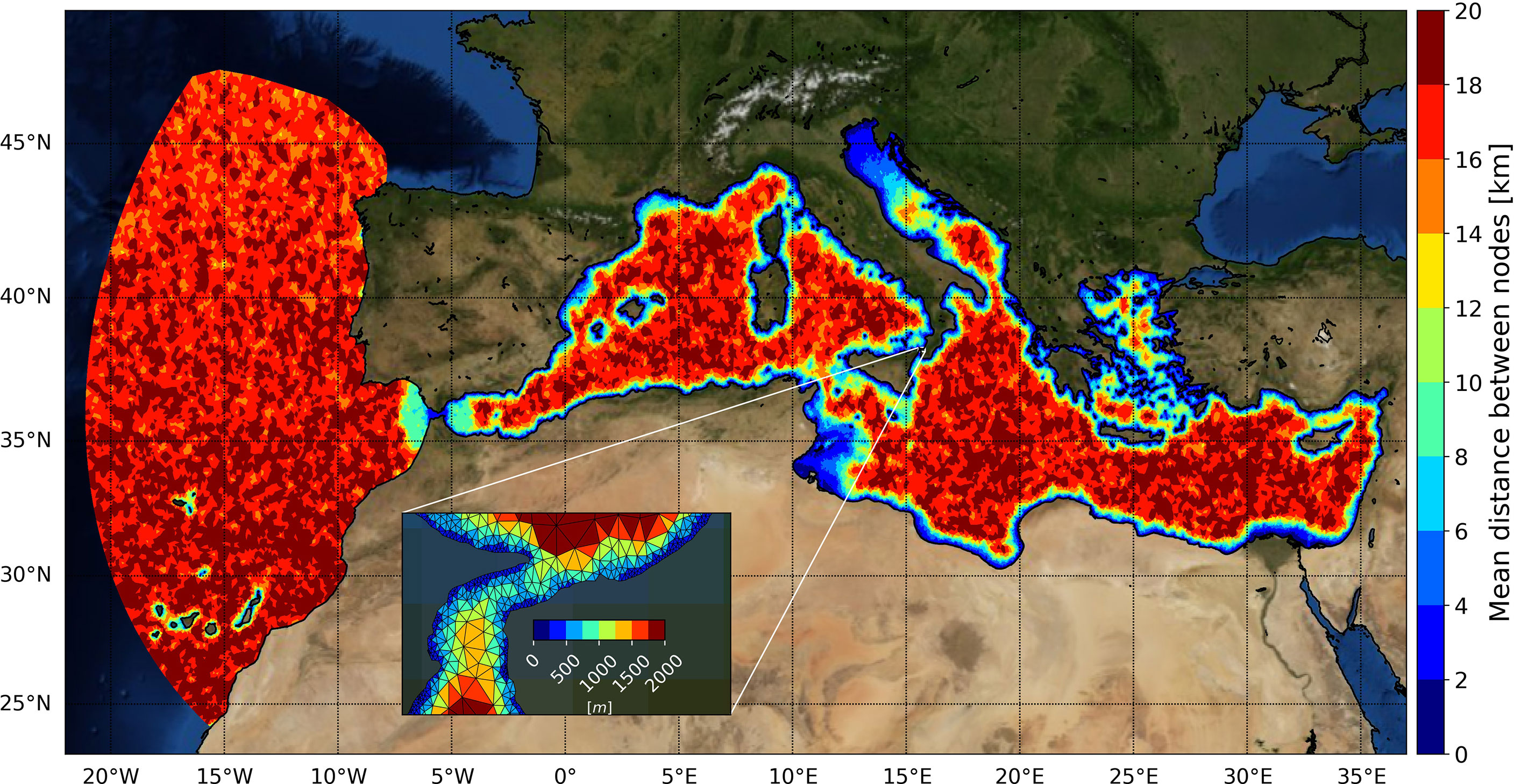
Figure 1 Mean distance (km) between nodes of the same element over the whole domain.

In recent years, hydrodynamic models have been used from global to regional scale, with increasing resolution and levels of complexity (for example, adding tide-surge coupling) (Vousdoukas et al. (2016); Fernández-Montblanc et al. (2020); Muis et al. (2020)) to assess coastal risks induced by storm surges, to overcome the lack of remote and in-situ observations. In particular, available tide gauges, wave buoys or satellite tracks in the Mediterranean Sea, does not allow to perform an exhaustive monitoring and description of sea surface elevation and significant wave height (H_S) evolution within the whole basin. This is especially true at the coast, where satellite-based observations are degraded. Provided that accurate atmospheric forcing fields (mainly depending on spatial resolution) exist, hydrodynamic simulations can reproduce satisfactorily the storm surge climate [e.g. Muis et al. (2020)]. The wave component is, however, misrepresented. So far, regional and global numerical hindcasts aimed at reproducing coastal extreme sea levels over large spatial scales only account for storm surges, neglecting waves. In shallow waters, the wind effect becomes dominant over pressure gradients for storm surge generation (Bertin et al., 2017; Joyce et al., 2019), but at the same time waves propagating towards the shoreline dissipate, mostly through viscous effects and depth-induced breaking. Wave radiation stress gradients (Longuet-Higgins and Stewart, 1964) also bring a non-negligible wave setup component that contributes to coastal extreme sea levels, to an extent that depends on nearshore varying wave transformation and morphological features of the coast. To address this issue when using a hydrodynamic model, wave setup has been historically added offline using bulk formulas, such as the very simplistic 0.2·H_S approximation (e.g. Vousdoukas et al. (2017)) or the empirical Stockdon formulation (Stockdon et al., 2006) that depends on the local slope and wave bulk parameters (e.g. Melby et al. (2012); Melet et al. (2018); Kirezci et al. (2020)). Other studies that focused on smaller areas and/or single events have included wave setup by dynamically simulating sea surface elevation by using a hydrodynamic-wave coupled model. For instance, using a such model in the Bay of Biscay, Bertin et al. (2015) performed two simulations, with and without waves under storm conditions. Results showed that extreme sea levels are locally increased by up to 40 cm when including the effect of waves on the coastal sea surface elevation, in the presence of offshore high waves (H_S between 7 to 10 m). Likewise, several local scale studies have revealed the importance to accurately represent the wave setup component for energetic wave storm events (Bertin et al., 2015; Pedreros et al., 2018; Lavaud et al., 2020; Pezerat et al., 2021).

Unlike its Atlantic counterpart where remotely-generated swell waves are common, the Mediterranean Sea is a wind-wave dominated environment (Ardhuin and Orfila, 2018; Toomey et al., 2018). Because of the complex orography and irregular coastline shape of the basin, wave-growth is limited by short fetches (Sayol et al., 2016), whereas wave setup effect is strongly dependent on the wave energy. Yet, Amores et al. (2020) showed that storm Gloria generated very high waves (H_S greater than 8 m measured by wave buoys), inducing wave setup that locally accounted for up to 40–50% of the total extreme sea levels along locations at the Spanish eastern coasts. Despite the absence of large swells as in the North Atlantic, risk-based storm surge assessments at Mediterranean scale should therefore be performed taking into account the effect of waves on sea surface elevation; otherwise coastal hazards linked to extreme sea levels are very likely to be underestimated.

Our objective here is to develop and present the dataset of Coastal Extremes in the Mediterranean Sea (CoExMed), a new storm surge and wind-wave hindcast generated using a hydrodynamic-wave coupled model, with a very high spatial resolution at the coast, along with an assessment of coastal hazards induced by these mechanisms in the Mediterranean Sea for the period 1950-2021. The paper is organised as follows: data and method used are described in detail in section 2, including the numerical model used for the generation and propagation of storm surges and waves and its configuration, in-situ and remote data used for the validation and the method employed to compute return levels. Model outputs (sea surface elevation and H_S) are evaluated against tide gauges, wave buoy and satellite data in section 3. Hazards induced by storm surges and waves are analysed at the Mediterranean scale through the computation of return levels in section 4. The last section summarises and discusses the results, and main conclusions are outlined.

2 Data and methods

2.1 Numerical modelling of storm surges and wind-waves

The fully-coupled hydrodynamic and wave model SCHISM (Zhang et al., 2016), an upgraded version of the original SELFE model (Zhang and Baptista, 2008), is used to perform the generation and propagation of storm surges and wind-waves over the Mediterranean Sea. The model allows to perform simulations with its 2DH barotropic mode alone (hydrodynamic simulation) and fully coupled (hydrodynamic-wave coupled simulation) with the spectral wave model WWM-III (Roland et al., 2012). Both modules share the same unstructured grid covering the whole Mediterranean basin, with an open boundary defined as a 15° semi-circle extending west from the Strait of Gibraltar (see Figure 1). The strait plays a key role in water exchanges between the Mediterranean Sea (e.g. tidal flows, along-strait wind setup) and the Atlantic Ocean; accounting for these processes is important to accurately simulate variations in sea surface elevation within the basin, especially for long periods of time. Indeed, pressure differences at both sides of the strait analysed in earlier works have revealed the role of the Atlantic Ocean on Mediterranean Sea level and circulation and, in particular, the influence of subinertial frequencies of the Gibraltar Strait barotropic flow (Candela, 1991; Le Traon and Gauzelin, 1997; García Lafuente et al., 2002). The model domain includes the western side of the Strait of Gibraltar to account for the region where alongshore winds induce Atlantic-Mediterranean wind driven sea level differences (Menemenlis et al., 2007). At the open boundary, the sea surface elevation is forced with the hydrostatic equilibrium formulation (the so-called inverted barometer effect), since atmospheric pressure is a major driver of barotropic sea level variability in the open ocean. Over the entire domain, the SCHISM model is forced with 10 m above sea level hourly wind fields and mean sea level pressure (1/4° spatial resolution) that are obtained from the ERA5 reanalysis dataset for the 1979-2021 period (Hersbach et al., 2020) and its recently released preliminary extension from 1950 to 1978 (Bell et al., 2021).

The unstructured computational grid is composed of 379,762 nodes shared by 649,326 elements, with a horizontal grid resolution ranging from ~ 20 km in the open ocean down to ~ 200 m at the coast. Figure 1 shows the domain grid and the mean distances between nodes, highlighting the progressively increasing spatial resolution from deep ocean towards the coast. The EMODnet Bathymetry (2018) with a grid resolution of 1/16 x 1/16 arc minutes (~115 x 115 m) is used. Such fine spatial resolution allows a reliable representation of wave-induced processes, considering the scale of the area of study, while ensuring a reasonable computational time. For both hydrodynamic and wave modules, the computational timestep is set to 10 minutes and outputs are stored every hour at all grid points. The surface wind stress is computed using a bulk formula of the drag coefficient following Pond and Pickard (2013). Using the same wind stress formulation for both hydrodynamic and hydrodynamic-wave coupled simulations allows to isolate the wave setup effect (temporal increase in mean water level due to breaking waves, see Section 4.1). For the bottom friction we assume a value of 0.02 for the Manning coefficient. In the Mediterranean Sea, as commented earlier, extreme coastal sea levels are mainly caused by storm surges rather than by the combination of tides and surges (Marcos et al., 2009), and therefore tides are not considered in the simulations. Nevertheless, given that tide-surge interactions are negligible in the basin, tidal oscillations can be added offline. The total wave spectral energy is distributed over 24 frequencies ranging from 0.04 to 1 Hz, and 24 directions from 0 to 360° (15° resolution). The hindcast has been performed using the Finisterrae II from the Centro de Supercomputación de Galicia (CESGA) facility. Each year was run separately with a 15 days spin-up, using 2 nodes for a total of 48 processors.

2.2 Observational data and model evaluation

Simulations are validated with in-situ and remote observations. Coastal sea surface elevation is compared with high-frequency tide gauge records from the recently updated GESLA3 dataset (paper available at Haigh et al., 2022, https://eartharxiv.org/repository/view/2828/). After removing duplicated tide gauge stations, a total of 93 tide gauges remained, with observations since 1950 and with an increasing number of available stations over time. For each tide gauge station and for theirentire period of operation, hourly non-tidal residuals are computed by removing the tidal signal on a yearly basis [using the Matlab UTide software (Codiga, 2022)]. Non-tidal residuals are then deseasoned by fitting the mean annual and semiannual components. Likewise, simulated waves are compared with records from in-situ wave buoys (hourly data) obtained from the Copernicus Marine Environment Monitoring Service (CMEMS, https://marine152.copernicus.eu/). This service provides in-situ observations in the Mediterranean Sea from 1985 to 2021. From every time series, outliers are removed manually after visual inspection of the observational record. In-situ wave observations are complemented with satellite measurements of H_S (dx~7km, dt~1s) from the ESA Sea State Climate Change Initiative (Dodet et al., 2020) covering the period 1991-2018.

For completeness, the outputs of coastal sea surface elevation are also compared with a state-of-the-art hydrodynamic model run. To do so, data from the Coastal Dataset for the Evaluation of Climate Impact (CoDEC, Muis et al. (2020)) are used. This simulation is based on the Global Tide and Surge Model Version 3.0 (GTSM) and simulates, at global scale, the generation and propagation of storm surges for the period 1979–2017. The spatial resolution along the Mediterranean coasts is 1.25 km.

2.3 Computation of return levels of coastal sea surface elevation and significant wave heights

For every coastal grid point of the model output (a total of 111561 nodes) we fit a Generalized Pareto Distribution (GPD) to a set of exceedances over a threshold. We choose the GPD instead of other extreme distributions following Wahl et al. (2017), who showed that it provides more stability to the computed return levels. In addition, it accommodates interannual variability in storminess much better than other distributions (e.g. GEV). We use maximum likelihood to fit the scale (σ) and shape (ξ) parameters of the theoretical distribution. To choose the threshold, we avoid the use of a common percentile to all grid points, as it may neglect the spatial variability of the storm hazards along the coasts. Instead, we define a suitable and independent threshold for every coastal point. To address this issue, Coles (2001) introduced the mean residual life plot (MRLP) method, a threshold selection technique involving a visual assessment that is strongly dependent of interpretation and therefore requires a subjective choice (see section 4.3.1, Coles (2001)). In addition, the author (see section 4.3.4 for more details, Coles (2001)) proposed another method assessing the stability of the GPD parameters. If a GPD is a reasonable model for excesses of a threshold u₀, excesses of a higher threshold u should also follows a GPD. Coles (2001) shows that for a threshold u>u₀ the corresponding scale parameter σ_u can be written:

$\begin{array}{ll}{\sigma }_u=\sigma u_0+\xi (u-u_0),& (1)\end{array}$

where ξ is the scale parameter (invariant to block size) and σ_u0 the GPD scale parameter for excesses over the threshold u₀. Pointing out that ξ is constant but that σ_u varies with u (except the case ξ=0), Coles (2001) defines a reparameterized GPD scale parameter

$\begin{array}{ll}\sigma *={\sigma }_u-\xi u,& (2)\end{array}$

that is constant (replacing equation (1) in (2)) for u>u₀. Therefore, u₀ is a good threshold estimate for fitting a GPD when the quantities ξ and σ* are stable for u>u₀. The latter has the advantage of providing results that minimise subjectivity and that has been so far used, either by itself or jointly with the MRLP method, in several studies (e.g. Yao and Zhu (2014); Hamdi et al. (2018); Kiriliouk et al. (2019)). Later on, Thompson et al. (2009) proposed an “Automated threshold selection technique” based on the stability of GPD parameters, that reduces even more the degree of interpretation. Let be u₀ a suitable threshold for a GPD fit. For u₀ ≤ u_i i + 1 (i ∈ [1,N] with N possible different thresholds sorted in ascending order), let be ${\widehat{\sigma }}_{u_i}$ and ${\widehat{\xi }}_{u_i}$ the maximum likelihood estimates of σ_ui and ξ_ui . It follows from (1),

$\begin{array}{ll}{\sigma }_{u_i}-{\sigma }_{u_{i-1}}=\xi (u_i-u_{i-1}).& (3)\end{array}$

Following the standard maximum likelihood theory discussed in Coles (2001) and properties on the expected value of maximum likelihood estimates ( $E[{\widehat{\sigma }}_{u_i}]={\sigma }_{u_i}$ and $E[{\widehat{\xi }}_{u_i}]={\xi }_{u_i}$), Thompson et al. (2009) defined, similarly to 2, the quantity

$\begin{array}{ll}{\tau }_{u_i}={\widehat{\sigma }}_{u_i}-{\widehat{\xi }}_{u_i}{u}_i& (4)\end{array}$

Combining maximum likelihood properties and equations 3 and 4, Thompson et al. (2009) shows that E[τ_ui−τ_ui−1] ≈ 0 and concludes that [τ_ui−τ_ui−1] approximately follows a normal distribution (see section 2.1 for more details, Thompson et al. (2009)).

In the present work, return levels are computed at every coastal grid point for both the sea surface elevation and H_S and for periods of 10, 20, 50, 100 and 200 years. Due to dissipation by bottom friction and wave breaking, coastal nodes are associated with the H_S value of the closest point but with depth greater than 20m, in order capture the high H_S. Time series of both variables are declustered by selecting local peaks with a three-day time-independent window (Cid et al., 2016; Vousdoukas et al., 2016). The above mentioned “Automated threshold selection technique” is applied using a minimum of 72 extreme events (corresponding to 1 per year) and up to 720 events (corresponding to 10 per year), to determine the most suitable threshold to these selected extreme events. The value is chosen as the first (lowest) threshold above which all values fulfill the condition of normality described above, as a function of [τ_ui−τ_ui−1].

3 Model validation against in-situ and remote data

The model evaluation against in-situ and remote observations is performed after selecting the simulated time series of the closest model grid point to each observational site. Note that the validation of the outputs with in-situ data is limited by the uneven geographical distribution of the observations. In particular, almost 90% of tide gauges used in this study are concentrated along Spanish, French and Italian coasts.

3.1 Coastal elevation

Figure 2 shows the non-tidal residual time series (red line) at 4 tide gauge stations (from West to East: Barcelona, Nice, Palermo, Alexandria) during year 2014, along with simulated sea surface elevation from this study (blue line) and from the GTSM model (Muis et al., 2020) (orange line). Overall, both simulations mimic observed sea level changes well, and generally share the same discrepancies with in-situ data. This is the case of, for example, the overestimated sea levels in June (06) at Barcelona (A) and Nice (B) tide gauge stations. We quantified the correspondence between model outputs and in-situ data using Root Mean Square Error (RMSE) and correlation. Figure 3 shows the results averaged yearly between 1980 and 2017 for all tide gauge stations available in every year (indicated in the bottom panel). RMSE has been calculated for the hourly record and also for independent events (non-tidal residual maxima values separated by at least 3 days). We observe that the number of tide gauges available (see lowest panel of Figure 3) for each year clearly increases with time and provides a statistically more robust validation of the modelled outputs in the recent period. Simulated coastal elevation shows good agreement with tide gauge signals, with a mean RMSE of 7 cm for hourly data, a mean RMSE of 7.2 cm for peak data and a mean correlation of 0.66. The numbers when GTSM is used to compare with observations remain nearly unchanged: RMSE of 6.9 cm, RMSE for independent events of 7.3 cm and correlation of 0.65. We can thus conclude that both model runs perform similarly when compared to tide gauge data. Over the whole period (1950-2021), the model maintains good performance when comparing simulated sea level to in-situ observations, with a mean RMSE of 7.5 cm for hourly data, a mean RMSE of 7.7 cm for peak data and a mean correlation of 0.64. The model performance at individual sites is evaluated using the Kling-Gupta Efficiency metric (KGE, Gupta et al. (2009)). This statistical indicator combines, in a unique criterion, the correlation, the standard deviation and the mean variability differences between observations and modelled outputs. A KGE value close to 1 means that the model reproduces perfectly the reality, while it performs very poorly when values are close to -0.41 (Knoben et al., 2019). Figure 4A shows the spatial validation of the coastal elevation at tide gauge sites. From one location to another, the KGE spatial pattern exhibits some differences. For instance, French tide gauges located in the Gulf of Lions show uniform high KGE values (up to 0.75) while a KGE ~0.50 is obtained for all tide gauges located along the Alboran Sea, being all the KGE values considerably higher than -0.41. However, there is no clear spatial variability in model performance, with an average KGE of 0.53. Finally, Figure 5A presents a quantile-quantile plot of simulated elevation againsttide gauges observations, taking into account entire time series. Quantiles indicate that the model slightly overestimates the sea surface elevation of non-tidal residuals below 70 cm, and slightly underestimates at higher values, most of them being located in the Adriatic Sea. Indeed, most extreme sea levels occurring in the Mediterranean Sea are found in the northern Adriatic Sea (Marcos et al., 2009), but also in the Gulf of Gabes (Conte and Lionello, 2014), where no tide gauge observations are available, highlighting the lack of in-situ data and model validation in some coastal sectors, especially in the southern coasts of the eastern Mediterranean.

FIGURE 2

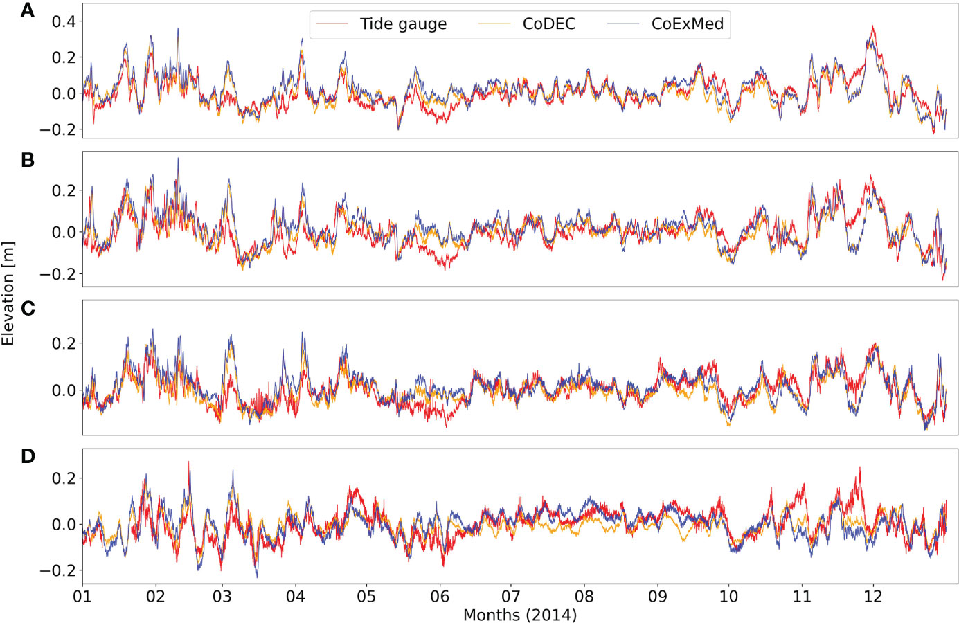
Figure 2 Sea surface elevation time series of tide gauges (red lines), CoExMed (blue lines) and CoDEC data (orange lines) at four different location: Barcelona (A), Nice (B), Palermo (C) and Alexandria (D).

FIGURE 3

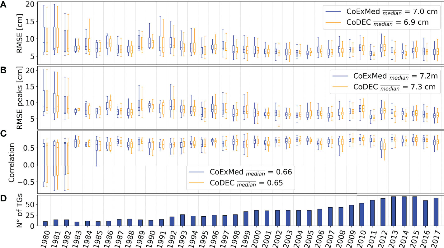
Figure 3 Analysis of differences observed between tide gauge signal and both simulated sea surface elevation from CoExMed (blue boxes and lines) and CoDEC (orange boxes and lines). The first three panels show annual boxplots for RMSE (A), RMSE peaks (B) and Pearson correlation coefficient (C) statistical indicators, and the median represents the mean of the median indicators. The box extends from the first to third quartile values of the data, with a line at the median. Lower (upper) whiskers are set to the first datum greater than Q1 - 1.5*IQR (Q3 + 1.5*IQR), where IQR is the interquartile range. The lowest panel (D) shows the annual number of tide gauges available.

FIGURE 4

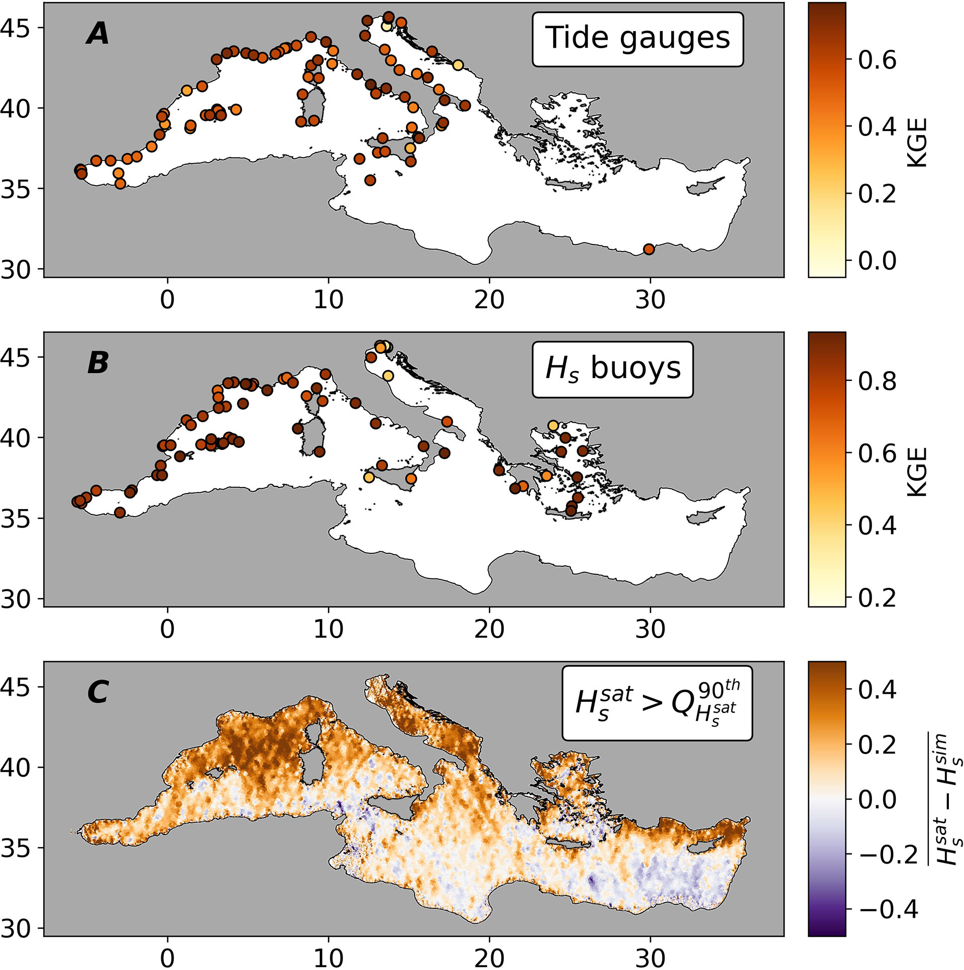
Figure 4 Spatial validation of modelled outputs against in-situ and remote observations. (A, B) respectively compare simulated coastal elevation to tide gauges and simulated H_S to wave buoy observations using KGE. (C) shows the 2D spatial mean bias between wave satellite observations ( $H_S^{sat}>{90}^{th}$ quantile) and the corresponding simulated H_S values.

FIGURE 5

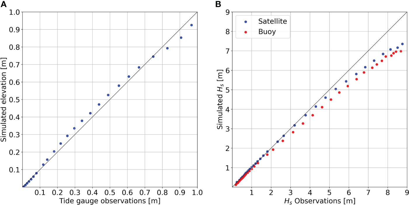
Figure 5 Quantile-quantile plot for sea surface elevation and H_S. Left (A) panel compares simulated elevation with tide gauges observations. Right (B) panel compares simulated H_S to both satellite (blue) and buoy (red) observations. Quantiles are firstly equally spaced with an 5 increment from 5^th to 95^th. For higher quantiles, the increment is divided by two at each iteration.

3.2 Significant wave height

As for sea surface elevation, we compare simulated H_S to wave buoys and satellite data. Figure 6 shows wave buoys time series (red line) at four different sites (from West to East: Melilla, Begur, Calvi, Heraklion) compared to simulated H_S (blue line). Again, the model reproduces almost perfectly the overall behaviour of observed H_S at wave buoys. However, a closer look reveals that simulated H_S presents some discrepancies for strongest events. In the same fashion as for non-tidal residuals, Figure 7 summarises the validation of H_S against wave buoys data from 1985 until 2020. The number of wave buoys available rises with time as well, with only 10 stations in 1995 and up to 55 in 2014. As suggested by Figure 6, except for the RMSE peaks (RMSE of values of local peaks previously extracted) higher than 1 m in 1985, simulated H_S shows good agreement with wave buoy signals, with a mean RMSE of 21.6 cm for hourly data, a mean RMSE of 41.9 cm for peaks and a mean correlation of 0.92. In the same way as for coastal sea level, simulated H_S is compared against wave buoys. Figure 4B shows KGE values at every buoy site. Highest KGE levels (up to 0.93) are concentrated in the western Mediterranean Sea while lower values are mainly found at stations located in the Adriatic and Aegean Seas (KGE as low as 0.24) where observed H_S levels are relatively low. Besides, KGE values are globally very high with an average of 0.77. In addition, and in order to compensate the limited in-situ wave data, especially in the southeastern Mediterranean, simulated H_S are compared to satellite measurements. Figure 4C shows the mean bias error (MBE) between satellite and simulated H_S. The computation of MBE only takes into account satellite H_S values greater than 90^th quantile and the corresponding modelled H_S at each grid node, to highlight extreme episodes. The model underestimates satellite H_S almost everywhere in the Mediterranean basin, except for the south part of the Levantine basin (~10-15 cm overestimation). Particularly, simulated H_S is lower than observed in the Adriatic Sea: this is a narrow semi-enclosed basin, where resolution might lead to misrepresentations of the atmospheric forcing (Barbariol et al., 2021). Furthermore, highest underestimations are found in the corridor situated in the area between the Balearic Islands and Sardinia characterized by a long-fetch where highest waves are usually found, generated by Northern and Mistral winds blowing over long distances. However, modelled H_S match well satellite H_S data with on average a mean bias error lower than 50 cm for relatively high waves (> 90^th quantile).

FIGURE 6

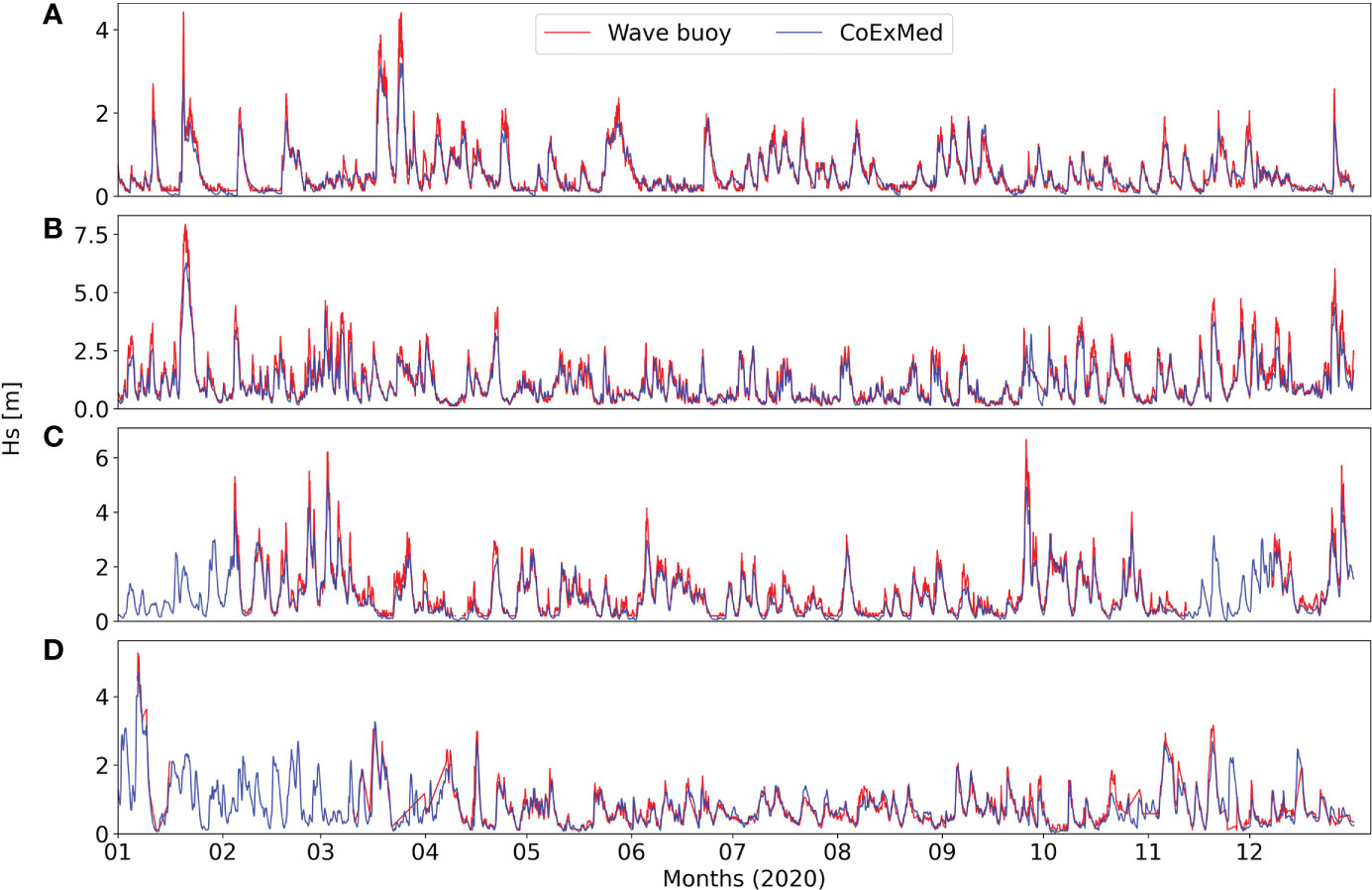
Figure 6 H_S time series of wave buoys (black lines) and simulated H_S at four different location: Melilla (A, -2.944E/35.327N), Begur (B, 3.64E/41.92N), Calvi (C, 8.65E/42.569N) and Heraklion (D, 25.0792E/35.4342N).

FIGURE 7

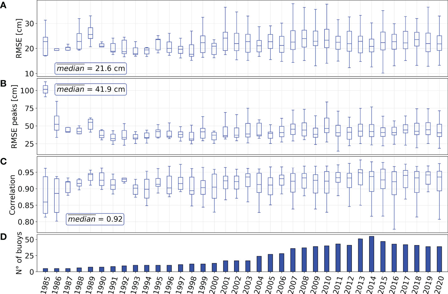
Figure 7 Boxplot analysis of differences observed between wave buoys signal and simulated H_S, using RMSE, RMSE peaks and Pearson correlation coefficient (first three panels). See Figure 3 for boxplot details. The lowest panel shows the annual number of wave buoy available.

The previously mentioned tendency of the model to underestimate observed H_S is illustrated in Figure 5B that shows a quantile-quantile plot of simulated and observed H_S, for both wave buoys (red dots) and satellite data (blue dots). The model performs very well for weak to moderate events, especially for satellite observations. In particular, the quantile-quantile analysis shows that simulated and satellite derived H_S match well (assuming a criteria of quantile difference lower than 25 cm) for waves below 4.80 m, whereas the model performs very well with respect to wave buoy data for H_S below 6 m. On the other hand, simulated H_S is underestimated for most intense events, up to 1.70 m for buoy observations and up to 1.40 m for satellite data for H_S higher than 8.5 m. Overall, quantile distribution shows very similar behaviour for both buoy and satellite data except for the upper tail, with varying differences observed for highest quantiles that are driven by a few extreme events like the Gloria storm that generated waves with H_S values greater than 8 m. The main difference between both sources of data is their spatial coverage: while satellite tracks provide observations all over the Mediterranean Sea, wave buoys are generally located close to the coast due to operational constraints. Likewise, the underestimation of modelled H_S for extreme events is reported in earlier studies that discuss different possible sources of error. In this respect, one possibility is linked to the horizontal resolution of the model grid, that is much finer than that of the atmospheric forcing (see part 2.1). Also, the limited resolution of wind forcing can be a main source of errors for wave model (Bertotti and Cavaleri, 2009). Finally, the ERA reanalysis dataset is reported to underestimate wind speed (Kalverla et al., 2020), especially for areas with complex orography (Jourdier, 2020) and for intense events like typhoons (Xiong et al., 2022).

4 Coastal hazards

4.1 The contribution of wave setup to extreme sea levels

We take advantage of the two complementary numerical simulations presented above to compute the contribution of wave setup to extreme sea levels. The present hindcast provides 72 years of both hydrodynamic and hydrodynamic-wave coupled simulations. The wave setup is obtained by simply subtracting the simulated sea surface elevation without waves (elev) to the simulated sea surface elevation with waves (elev^coupled); so it contains not only the contribution of the waves but also the coupling with the atmospheric pressure and wind.

Figure 8 provides two examples of wave contribution to coastal sea surface elevation. The first case shows a snapshot (day 20 at 07:00) of simulated sea surface elevation (Figures 8C, D) and H_S (Figure 8A) during Storm Gloria that hit the Spanish eastern coasts (see wide area in Figure 8A) in January 2020 (Amores et al., 2020; de Alfonso et al., 2021). During this event, extremely large waves were recorded by wave buoys (with H_S over 8 m) that notably propagated towards coasts of the Comunidad Valenciana (Spain) with perpendicular direction to shoreline (area zoomed, see Figure 8A) generating significant coastal inundation and numerous damages. This area is characterised by a shallow continental shelf that extends beyond 10 km offshore (30 m depths are reached at this distance, see Figure 8B), with the wind effect becoming dominant over atmospheric gradient pressure contribution to storm surges (Bertin et al., 2017) and shallow waters favouring depth-induced wave breaking. Lower panels (Figures 8C, D) show simulated elev (C) and elev^coupled (D). With only the combination of inverse barometer and wind setup contributions, simulated elev reaches 40 cm and displays a uniform pattern along the coast. When the wave generation and propagation are added, elev^coupled increases up to 70 cm (D). The amplitude of waves and local depth explain the observed spatial differences on the coast. Overall, the contribution of wave setup to simulated coastal elevation is significant (up to 120% increase) in this case. Since this storm was an extraordinary event in terms of intensity, another example of a less energetic event is shown in Figure 8 (Case N°2) in order to illustrate the ability of the hindcast to capture wave setup also during weaker storms or undocumented events. For instance, our simulation reproduces the generation and propagation of a wave storm that hit the southern Sicilian coasts (Italy) in December 2004. During this event, winds towards northeast generated H_S higher than 4 m along the coast (see Figure 8E, Case N°2). In the same way as for the first case, Figure 8 displays a snapshot (day 26 at 21:00) of sea surface elevation without (G) and with waves (H). To a lesser extent than for storm Gloria, the contribution of waves to coastal extreme sea levels is evidenced. Indeed, simulated elev hardly surpasses 20 cm for the southern coasts, while the elev^coupled reaches 40 cm when the wave setup contribution is accounted for. Here, the storm conditions and the bathymetry are different from the previous example, with smaller waves and a narrower continental shelf. Thereby, these two case studies show the ability of the model to capture the imprint of wave effect on sea surface elevation under varying conditions.

FIGURE 8

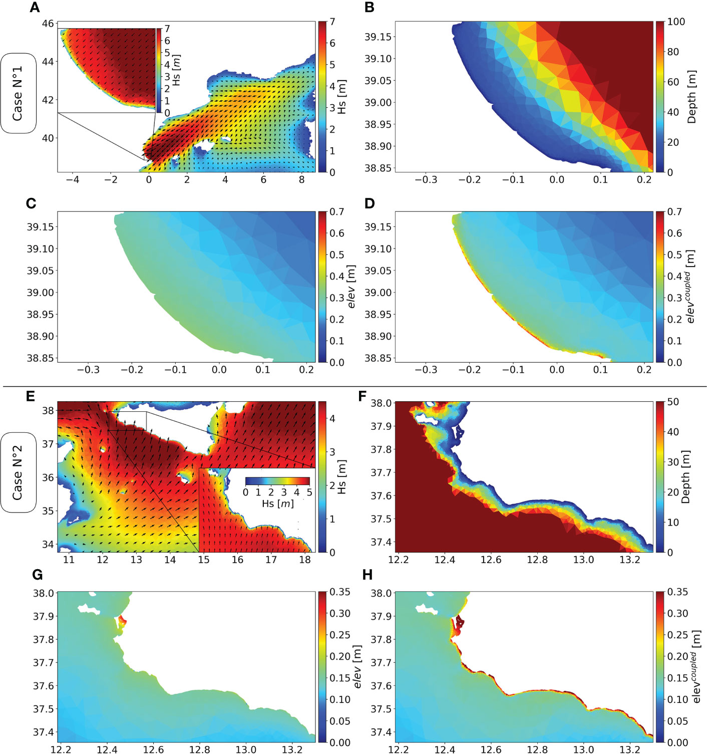
Figure 8 Snapshots of simulated sea surface elevation and H_S generated by two independent storms. Case N°1 corresponds to the Gloria storm that hit eastern Spanish coasts in January 2020 (snapshot on day 20, at 07:00). Case N°2 corresponds to a wave storm that impacted southern coast of Sicily in December 2004 (snapshot on day 26, at 21:00). For both cases, upper left panel (A, E) shows simulated H_S for a large area and a zoom of a smaller zone within it. Upper right (B, F), lower left (C, G) and lower right (D, H) panels show respectively the bathymetry, the elev and the elev^coupled of the zoomed area.

In order to have a more exhaustive insight of the model ability to capture wave setup at the Mediterranean scale, we analyse the contribution of wave setup for extreme events defined over the corresponding threshold (see section 2.3) at every coastal grid point. To do so, we subtract elev from elev^coupled for each event. Figure 9 shows the 99^th quantile (1% of highest values) of the resulting wave setup during extremes. It should be reminded that because of the very high density of coastal points (111561), Figure 9 (along with Figures 10, 11A, B) does not show exhaustively all coastal points, as there are inevitably overlapping nodes at this scale. Large wave setup values are found in different areas of the western, central and eastern Mediterranean Sea. Highest levels are found in the Adriatic (eastern coasts), around the Gulf of Gabes in northern Tunisia and western Sardinia coasts. As a consequence of the first example discussed above with Storm Gloria, one of the strongest events ever recorded, the imprint of wave setup is clearly observed in the eastern Spanish coasts (Case N°1). The same applies to the southern coasts of Sicily (Case N°2). In the rest of the coastal regions within the basin, wave setup below 10 cm is found (e.g. North of the Alboran sea, Spanish and French coasts, Aegean sea). Due to their particular characteristics (wave energy and direction, morphological characteristics of the zone, depth of coastal and near-shore nodes or spatial resolution are crucial for the model to capture wave setup induced by wave breaking), these regions are not prone to the development of important wave setup. Overall, the imprint of potential contribution of wave setup to coastal sea surface elevation is well captured by the model along many coastlines of the Mediterranean.

FIGURE 9

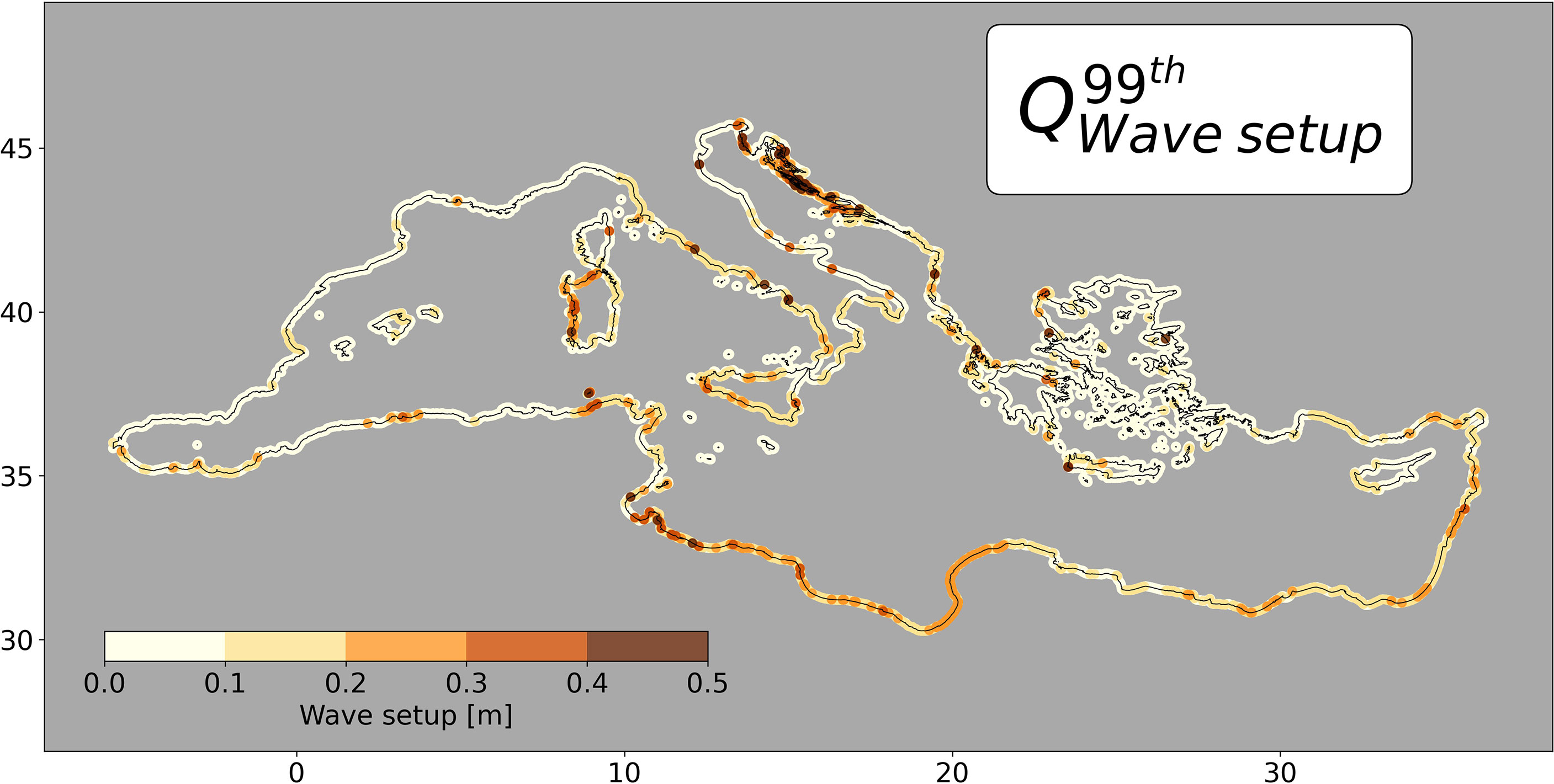
Figure 9 Wave setup (elev^coupled-elev) 99^th quantile of sea surface elevation of independent events (see section 2.3) for coastal grid points within the Mediterranean Sea.

FIGURE 10

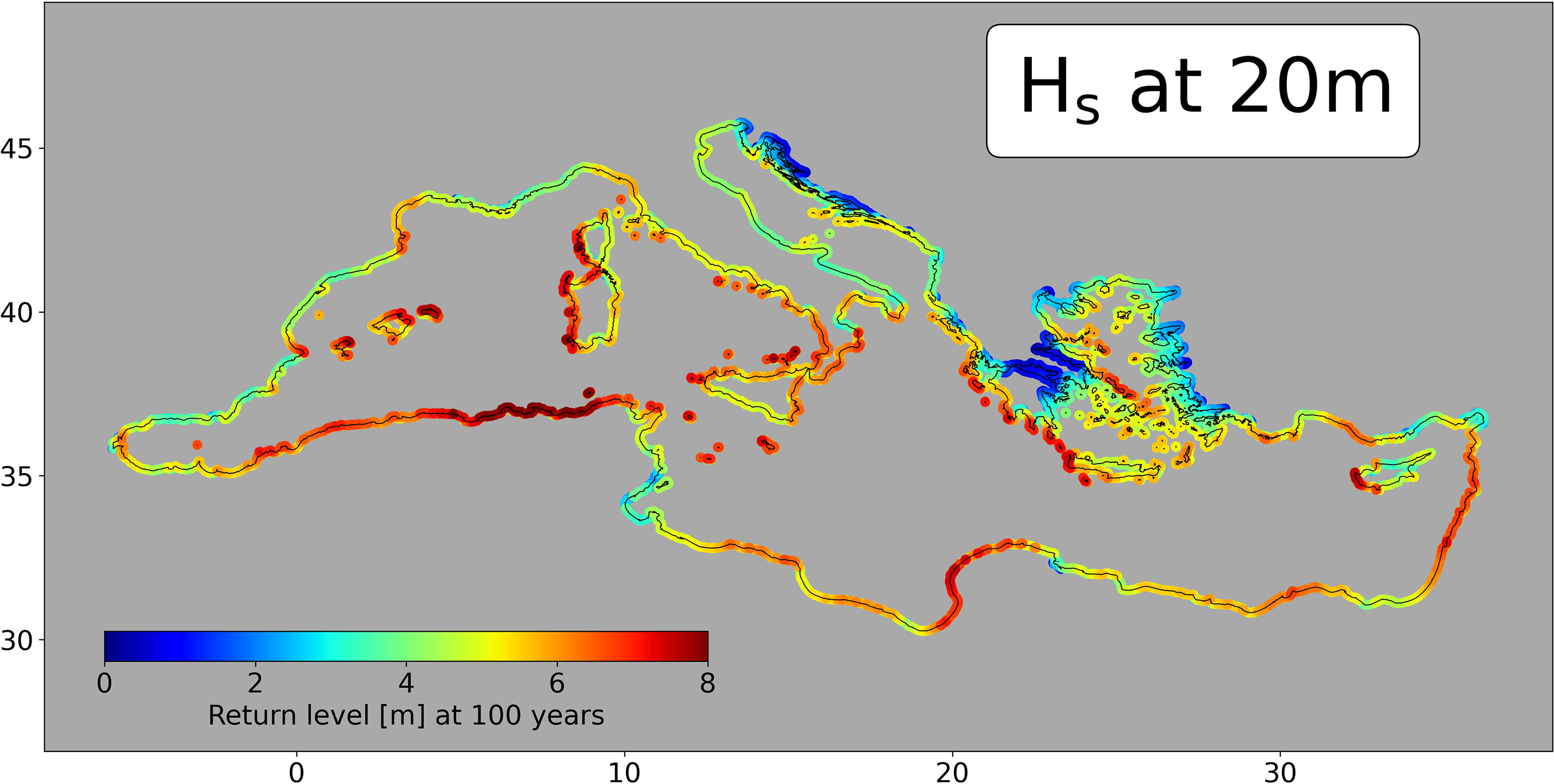
Figure 10 100-year return levels of H_S at 20 m for Mediterranean coasts, islands included.

FIGURE 11

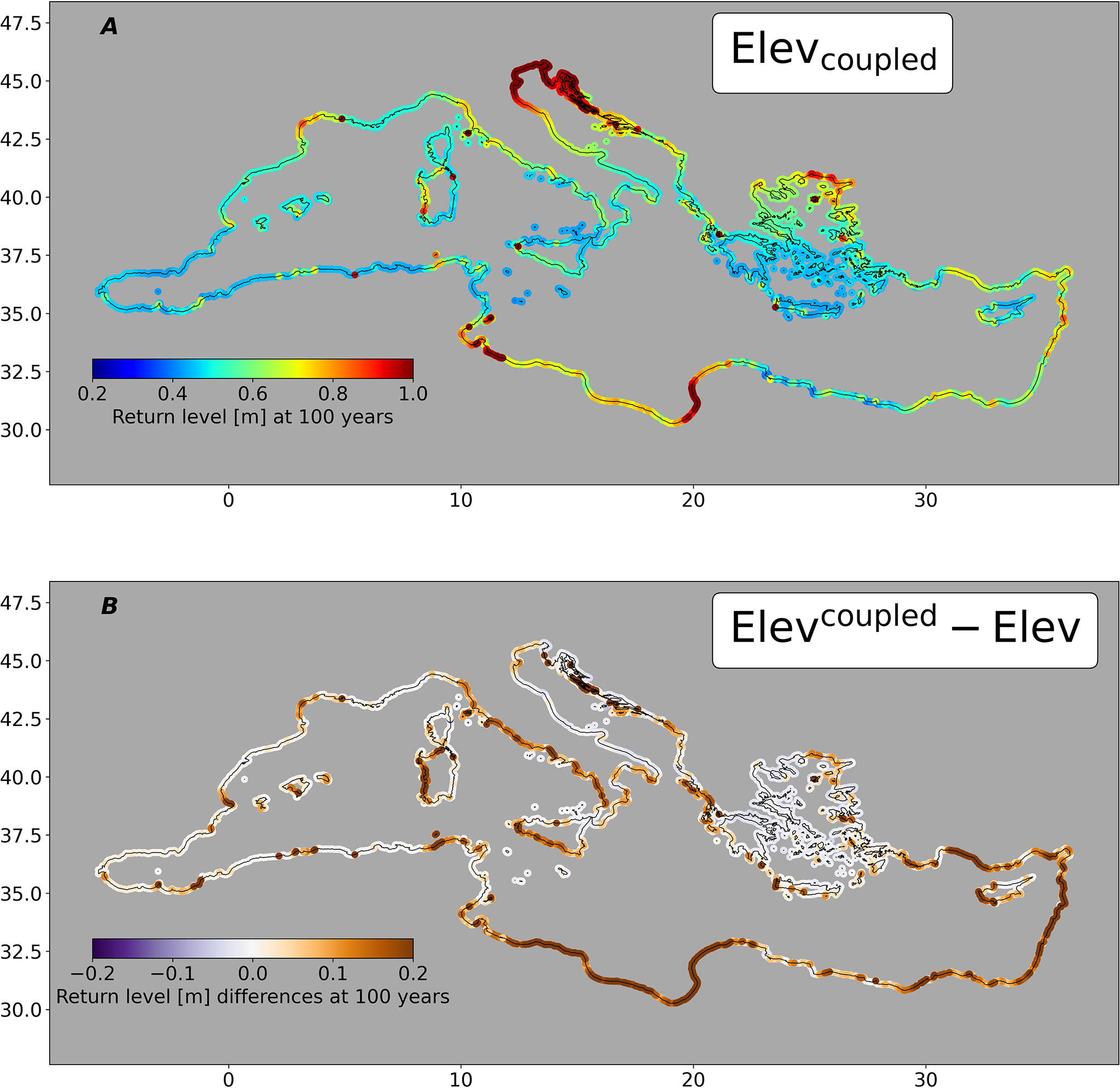
Figure 11 100-year return levels of sea surface elevation for Mediterranean coasts, islands included. Upper panel (A) shows return levels for elev^coupled. Lower panel (B) shows the difference between return levels computed from extreme event distributions of elev^coupled and elev.

4.2 Return levels

The quantification of the hazards of waves and extreme sea levels along Mediterranean coasts is investigated in this section in terms of return levels. For every coastal grid point and for both elev^coupled, elev and H_S at 20 m, we compute return levels using a GPD method with thresholds chosen after applying the automated threshold selection technique presented in section 2.3 to the distribution of selected extreme events described in section 2.3. The resulting 100-year return levels are mapped in Figure 10 for H_S and Figures 11A, B for the elev^coupled and elev.

The spatial pattern of 100-year return level of H_S reflects the large waves that can be found in the central western Mediterranean basin, from the Gulf of Lions, around the Balearic islands, through west of Sardinia and down until the northern coast of Algeria, where return levels greater than 8 m are found. High values of H_S return levels, between 6 m and 8 m, are also observed in the eastern Mediterranean (e.g. southern Italy and Greece, Lybian and Egyptian northern coasts, East of Cretes and Israel). Overall, a total 48.4% of coastal grid points show 100-year return levels greater than 4 m. Lower values correspond to areas with limited fetch (distance over which wave-generating wind blow). For instance, values below 1 m are found in the Adriatic Sea, especially along the Croatian coastline (north Adriatic) that is protected by a belt of islands. Similarly, the numerous islands within the Aegean sea prevent waves from growing and propagating. Furthermore, low to moderate H_S return levels, with values between 2 m and 4 m, are found in the Gulf of Gabes (Tunisian coasts, around 10°E/34°N). Othmani et al. (2017) described this area as an extended shallow region, with depths of 50 meters found 110 km offshore (400 km from the coasts for depths of 200 m). Therefore, the propagation and growth of waves is limited since wave breaking point is reached for waves with relatively low period and amplitude (nonetheless inducing wave setup).

Figure 11A maps 100-year return levels of elev^coupled, while Figure 11B shows the differences between 100-year return levels of elev^coupled and 100-year return levels of elev. The spatial distribution of the return levels clearly highlights geographical zones with values over 1 m. The largest values of return levels are observed in the Adriatic Sea with a quite uniform spatial distribution over its northern part (up to 1.30 m in the Marano Lagoon, Italy), from the Venice area until Trieste in Italy. This region is located at the tail of the longest fetch of the Sirocco wind, that is generated by air-pressure gradients linked to Mediterranean low-pressure systems crossing the Adriatic Sea (Medugorac et al., 2018). Thereby, the Sirocco blowing from southeast often generates storm surges in the north of the Adriatic (Italian coasts), where the wind contribution to coastal elevation is dominant over wave setup and inverse barometer contributions. Indeed, Figure 11B reveals a small contribution of wave setup to 100-year return levels, with differences lower than 9 cm (8% increase respect to elev 100-year return level). In such semi-enclosed basin, wave generation and growth is restricted due to a limited fetch in comparison to the corridor in the western basin. Moreover, Figure 9 shows that wave setup 99^th quantiles lower than 10 cm are mainly found for the northern and western part of the Adriatic. The geographical pattern of the return levels shows that high values are generally found with the presence of wide continental shelves with mild slopes that favour the wind setup contribution to storm surge generation, which dominates over inverse barometric effect (Bertin et al., 2017) and wave setup component with little depth inducing wave-breaking. This is the case of the Gulf of Lions and of the coastline sector between the Gulf of Gabes and the northern coasts of Lybia (e.g. Gulf of Syrte). For the latter area, there is an apparent and significant correlation of high return level of elev^coupled (see Figure 11A) with levels of wave setup observed in Figure 9. This relationship is confirmed in Figure 11B that represents the contribution of waves to extreme sea levels. Larger positive values of these differences are found at regions with wave setup. For instance, 100-year elev^coupled return levels are found to be up to 40 cm higher than 100-year elev returnlevels in the Gulf of Syrte, which represents an increase of more than 60%. Also, as expected from results in section 4.1, 100-year return levels of sea surface elevation when accounting for waves are higher in the areas of Spanish eastern coast (Case N°1) and south Sicily (Case N°2) with up to 25-30 cm (~60% respect to elev 100-year return levels) and 15-20 cm increase (~50% respect to elev 100-year return levels), respectively. As it has been shown in previous studies such as Marcos et al. (2019), wave setup is a relevant mechanism that can lead to significant changes when computing extreme sea level return levels. For instance, in the area impacted by storm Gloria (beach of Gandia, eastern Spanish coast), the uncoupled modelled elev leads to an extreme sea level of 46 cm expected once every 100 years, while its frequency decreases down to once every 8 years when accounting for wave setup component (elev^coupled). Overall, the values of 100-year return levels of elev^coupled exceed 50 cm in 42.8% of coastal grid points, including regions as the Aegean Sea, Eastern Sardinia or coasts in the Levantine basin.

5 Discussion and conclusion

This work presents CoExMed, a new Mediterranean hydrodynamic-wave coupled hindcast with an unprecedented spatial resolution and period covered (1950-2021), that includes, for the first time, the wave setup component along the coasts that contributes to the coastal extreme sea levels (up to more than 100%). The modelled storm surges and waves have shown a very good skill when compared with in-situ and remote observations. The length and completeness of the hindcast permits the accurate computation of extreme sea level statistics along the Mediterranean coasts separating geographical features due to its high spatial resolution. The results have thus direct applications in coastal impact studies, can be used to feed local models and to assess with increased accuracy coastal hazards.

Extreme ocean waves growth occurs under conditions of combined sustained winds and long fetch (Lionello et al., 2006). Compared to the Atlantic Ocean and because of its very complex orography, the Mediterranean Sea is a region where the generation and propagation of large waves is limited by short fetches. However, powerful waves greater than 6 m occur in the Mediterranean Sea (Lionello et al., 2006; Amores et al., 2020). In agreement with other studies focusing on the Mediterranean wave climate (Lionello et al., 2006; Soukissian et al., 2017; Morales-Márquez et al., 2020; Elkut et al., 2021), our results show that highest waves are mainly found in the long fetch corridor between the Gulf of Lions southwards to the Algerian coasts, generated by northerly dominant winds (Mistral and Tramuntana) and enchancedby orographic effect (Menéndez et al., 2013). Although the spatial patterns are well reproduced in the hindcast, the comparison of modelled waves to buoy and satellite data reveals that extreme wave heights are underestimated (see part 3.2). This fact is also reported in the recent work of Barbariol et al. (2021) that provides a 40-years (1980–2019) wave hindcast, obtained by combining the ERA5 reanalysis wind forcing with the state-of-the-art WAVEWATCH III spectral wave model and that was compared to H_S satellite altimeter observations. Apart from the western Mediterranean, Barbariol et al. (2021) found high waves in the central Mediterranean (From the Ionian Sea southwards to Tunisian and Lybian coasts) in agreement with our results. H_S return levels presented in section 5 also exhibit the presence of high waves within the central Mediterranean. Indeed, Figure 10 shows that high 100-year return levels of H_S (between 5 m and more than 8 m) are found for the surrounding coasts of the central Mediterranean, especially for the southwest coasts of Greece and northern Lybian coasts. Our results show as well high return levels of H_S for the eastern Mediterranean (western coasts of Cyprus island, Israel, Liban and Syria), in line with Barbariol et al. (2021), yet to a lesser extent, during the summer season.

The overall evaluation of the simulated sea surface elevation against tide gauges showed good agreement (see section 3.1), with a performance very similar to other earlier studies (e.g. Muis et al. (2020)). As commented earlier, extreme sea levels are mainly driven by atmospheric forcing (atmospheric gradient pressure and wind effects) and wave setup. However, using the SCHISM model in its 2DH horizontal barotropic configuration does not allow the representation of mesoscale eddies, being a potential source of error for sea surface elevation simulation. Investigating the role played by mesoscale eddies and its importance to reproduce the evolution of sea surface elevation requires to run the model in its 3D configuration, which is not feasible due to computational constraints (high spatial resolution and long simulation period). Though the latter can be investigated in future works using for instance altimetry data, it is not in the scope of this study to assess the contribution of mesoscale eddies to extreme sea levels and more broadly sea surface elevation. Importantly, during extreme weather events, the hindcast also accounts for the wave setup effect along with storm surges, thus increasing coastal extreme sea levels. We also demonstrate that this contribution is widespread in the Mediterranean basin (see section 4.1). In a recent study, Toomey et al. (2022) used the hydrodynamic wave coupled SCHISM model to investigate the impact of Medicanes occurring over the Mediterranean sea, performing a regional coastal hazards assessment for the present and future climates. Overall, medicane-induced waves and storm surges showed poor spatial correlation between waves and sea surface elevation patterns, though waves greater than 14 m were generated. With a 10 times higher resolution (a 2 km coastal spatial was used in the work of Toomey et al. (2022)), the present hindcast shows a better ability for capturing the wave setup imprint at Mediterranean scale. For instance, eastern coasts of Sardinia show high return levels of wave setup (greater than 30-40 cm) while in spite of very high Medicane-generated H_S, Toomey et al. (2022) results showed very low 100-year return levels of storm surges (see Figure 12), highlighting the advantage of having high spatial resolution for wave setup generation. As commented in section 4.1, wide and gently sloping continental shelves favour wind effect contribution to total water level and also wave setup with shallow depths inducing wave-breaking. For the latter, very high spatial resolution is not paramount since the continental shelf extends over relatively long distance. However, the resolution parameter becomes essential for coasts characterised by a narrower continental shelf or simply the absence of it. In such areas, the wave setup contribution to coastal sea level extremes becomes dominant over the wind effect contribution {Bertin et al., 2017; Joyce et al., 2019) like in the case of volcanic islands (e.g. Hawaiian Islands, Kennedy et al. (2012)]. In that way, the present high resolution wave and storm surges hindcast addresses this issue and points out the importance to adapt the spatial resolution to the morphological characteristics of the area studied, though along the very diversified Mediterranean coastlines the wave setup component is ineluctably likely to be underestimated or not captured. With the current spatial resolution, we identify regions where wave setup plays a role in coastal extreme sea levels; nevertheless, this does not exclude that this effect may be also relevant in other regions for which a higher resolution would be needed. Our results are, therefore, conservative in that sense.

A possible source of error when it comes to wave modelling, and thereby wave setup representation, is the physical formulation of sea the surface stress. Bertin et al. (2015) and Pineau-Guillou et al. (2020) investigated the impact (during storms occurring in the Bay of Biscay and the North Sea, respectively) of using a wave dependent rather than an only wind dependent formulation for surface stress computation, resulting in more accurate modelled sea surface elevation under conditions of young and rougher sea state (as it happens in the Mediterranean Sea because of its limited fetch). As commented in section 2.1, the Pond and Pickard (2013) bulk formula was used in this study to allows us to isolate the wave setup effect. However, following Bertin et al. (2015) and Pineau-Guillou et al. (2020) findings, we ran simulations over the 2015-2020 period with a wave dependent surface stress (as used in Bertin et al. (2015)) and compared results to our simulated hindcast over this time period. Overall, RMSE and correlation statistical indicators did not show any clear improvement or downgrade for the validation of simulated sea surface elevation compared to tide gauges (hindcast data), with a mean RMSE of 6.7 cm (6.8 cm), a mean RMSE for peak data of 6.8 cm (6.7 cm) and a mean correlation of 0.684 (0.687). In parallel, statistical indicators for the comparison to wave buoys data showed no changes at all. Although we do not discard that a wave dependent formulation may have significant influence for single events, it has no incidence in the scope of this study that is to characterise storm surges and wave climate over more than 70 years.

This contribution with a new hydrodynamic-wave coupled generated hindcast is innovative in many ways. Taking advantage of the ERA5 dataset covering the 1950-2021 period, we produced, to our knowledge, the longest model-based climatology of both wind-waves and sea surface elevation within the Mediterranean basin. Moreover, statistical analysis robustness (e.g. for the computation of return levels for long return periods) is enhanced when leaning on such large time series of storm surges and H_S. Finally, the possibility to extract the imprint of the wave setup component within the entire Mediterranean basin at unprecedented high resolution along the coast reveals very interesting avenues for future research, knowing for instance that wave setup contributions to storm surges are often taken into account through the use of bulk formulas.

Data availability statement

Data from this study can be requested to authors. Return levels at 10, 20, 50, 100 and 200 years, for both coastal sea surface elevation and Hs variables, are available at the Zenodo repository 10.5281/zenodo.6802090.

Author contributions

TT and MM designed the work. TT performed the numerical simulations with inputs from AA. All authors contributed to the interpretation and discussion of the results. All authors contributed to the article and approved the submitted version.

Funding

This study was supported by the Project RTI2018-093941-B-C31 funded by MCIN/AEI/10.13039/501100011033/and by FEDER Una manera de hacer Europa. Tim Toomey acknowledges an FPI grant associated with the MOCCA project (grant number PRE2019-088046). Angel Amores was funded by the Conselleria d’Educació, Universitat i Recerca del Govern Balear through the Direcció General de Política Universitària i Recerca and by the Fondo Social Europeo for the period 2014–2020 (grant no. PD/011/2019).

Acknowledgments

The authors are grateful to Dr Sanne Muis for sharing the CoDEC data, to Dr Xavier Bertin, Dr Marc Pezerat, Dr Thomas Wahl and Dr Alejandra R. Enríquez for discussing the outputs of the reanalysis, and to Dr Y. Joseph Zhang for his assistance with the SCHISM modelling system.

Conflict of interest

The authors declare that the research was conducted in the absence of any commercial or financial relationships that could be construed as a potential conflict of interest.

Publisher’s note

All claims expressed in this article are solely those of the authors and do not necessarily represent those of their affiliated organizations, or those of the publisher, the editors and the reviewers. Any product that may be evaluated in this article, or claim that may be made by its manufacturer, is not guaranteed or endorsed by the publisher.

References

Amores A., Marcos M., Carrió D. S., Gómez-Pujol L. (2020). Coastal impacts of storm gloria (january 2020) over the north-western mediterranean. Natural Hazards. Earth Syst. Sci. 20, 1955–1968. doi: 10.5194/nhess-20-1955-2020

CrossRef Full Text | Google Scholar

Ardhuin F., Orfila A. (2018). Wind Waves, in: New Frontiers in Operational Oceanography, edited by: Chassignet E., Pascual A., Tintoré J., Verron J., GODAE OceanView, Florida State University College of Medicine, chap. 14, 393–422. doi: 10.17125/gov2018.ch14

CrossRef Full Text | Google Scholar

Barbariol F., Davison S., Falcieri F. M., Ferretti R., Ricchi A., Sclavo M., et al. (2021). Wind waves in the mediterranean sea: An era5 reanalysis wind-based climatology. Front. Mar. Sci. 8. doi: 10.3389/fmars.2021.760614

PubMed Abstract | CrossRef Full Text | Google Scholar

Bell B., Hersbach H., Simmons A., Berrisford P., Dahlgren P., Horányi A., et al. (2021). The era5 global reanalysis: Preliminary extension to 1950. Q. J. R. Meteorol. Soc. 147, 4186–4227. doi: 10.1002/qj.4174

CrossRef Full Text | Google Scholar

Bertin X., Li K., Roland A., Bidlot J. (2015). The contribution of short-waves in storm surges: Two case studies in the bay of biscay. Continental. Shelf. Res. 96, 1–15. doi: 10.1016/j.csr.2015.01.005

CrossRef Full Text | Google Scholar

Bertin X., Olabarrieta M., McCall R. (2017). “Hydrodynamics under storm conditions,” in Coastal storms: Processes and impacts. Ed. et Giovanni Coco P. C. (John Wiley & Sons Ltd).

Google Scholar

Bertotti L., Cavaleri L. (2009). Large And small scale wave forecast in the mediterranean sea. Natural Hazards. Earth Syst. Sci. 9, 779–788. doi: 10.5194/nhess-9-779-2009

CrossRef Full Text | Google Scholar

Candela J. (1991). The gibraltar strait and its role in the dynamics of the mediterranean sea. Dynamics. Atmospheres. Oceans. 15, 267–299. doi: 10.1016/0377-0265(91)90023-9

CrossRef Full Text | Google Scholar

Cid A., Menendez M., Castanedo S., Abascal A., Mendez F., Medina R. (2016). Long-term changes in the frequency, intensity and duration of extreme storm surge events in southern europe. Climate Dynamics. 46, 1503–1516. doi: 10.1007/s00382-015-2659-1

CrossRef Full Text | Google Scholar

Codiga D. (2022). UTide Unified Tidal Analysis and Prediction Functions. MATLAB Central File Exchange Available at: https://www.mathworks.com/matlabcentral/fileexchange/46523-utide-unified-tidal-analysis-and-prediction-functions.

Google Scholar

Coles S. (2001). “An introduction to statistical modeling of extreme values,” in Springer series in statistics (London: Springer-Verlag).

Google Scholar

Conte D., Lionello P. (2014). Storm surge distribution along the mediterranean coast: Characteristics and evolution. Proc. - Soc. Behav. Sci. 120, 110–115. doi: 10.1016/j.sbspro.2014.02.087

CrossRef Full Text | Google Scholar

de Alfonso M., Lin-Ye J., García-Valdecasas J. M., Pérez-Rubio S., Luna M. Y., Santos-Muñoz D., et al. (2021). Storm gloria: Sea state evolution based on in situ measurements and modeled data and its impact on extreme values. Front. Mar. Sci. 8. doi: 10.3389/fmars.2021.646873

PubMed Abstract | CrossRef Full Text | Google Scholar

Dodet G., Piolle J.-F., Quilfen Y., Abdalla S., Accensi M., Ardhuin F., et al. (2020). The sea state cci dataset v1: Towards a sea state climate data record based on satellite observations. Earth Syst. Sci. Data 12, 1929–1951. doi: 10.5194/essd-12-1929-2020

CrossRef Full Text | Google Scholar

EMODnet Bathymetry Consortium (2018). MODnet Digital Bathymetry (DTM 2018). doi: 10.12770/18ff0d48-b203-4a65-94a9-5fd8b0ec35f6

CrossRef Full Text | Google Scholar

Elkut A. E., Taha M. T., Abu Zed A. B. E., Eid F. M., Abdallah A. M. (2021). Wind-wave hindcast using modified ecmwf era-interim wind field in the mediterranean sea. Estuarine. Coast. Shelf. Sci. 252, 107267. doi: 10.1016/j.ecss.2021.107267

CrossRef Full Text | Google Scholar

Fernández-Montblanc T., Vousdoukas M., Mentaschi L., Ciavola P. (2020). A pan-european high resolution storm surge hindcast. Environ. Int. 135, 105367. doi: 10.1016/j.envint.2019.105367

PubMed Abstract | CrossRef Full Text | Google Scholar

Fritz H. M., Blount C., Sokoloski R., Singleton J., Fuggle A., McAdoo B. G., et al. (2007). Hurricane katrina storm surge distribution and field observations on the mississippi barrier islands. Estuarine. Coast. Shelf. Sci. 74, 12–20. doi: 10.1016/j.ecss.2007.03.015

CrossRef Full Text | Google Scholar

García Lafuente J., Álvarez Fanjul E., Vargas J. M., Ratsimandresy A. W. (2002). Subinertial variability in the flow through the strait of gibraltar. J. Geophys. Res.: Oceans. 107, 32–1–31–9. doi: 10.1029/2001JC001104

CrossRef Full Text | Google Scholar

Gupta H. V., Harald K., Yilmaz K. K., Martinez G. F. (2009). Decomposition of the mean squared error and nse performance criteria: Implications for improving hydrological modelling. J. Hydrol. 377, 80–91. doi: 10.1016/j.jhydrol.2009.08.003

CrossRef Full Text | Google Scholar

Haigh I. D., Marcos M., Talke S. A., Woodworth P. L., Hunter J. R., Hague B. S., et al. (2022). GESLA Version 3: A major update to the global higher-frequency sea-level dataset. Geoscience Data Journal, 00, 1–22. doi: 10.1002/gdj3.174

CrossRef Full Text | Google Scholar

Hamdi Y., Garnier E., Giloy N., Duluc C.-M., Rebour V. (2018). Analysis of the risk associated with coastal flooding hazards: A new historical extreme storm surges dataset for dunkirk, france. Natural Hazards. Earth Syst. Sci. 18, 3383–3402. doi: 10.5194/nhess-18-3383-2018

CrossRef Full Text | Google Scholar

Hersbach H., Bell B., Berrisford P., Hirahara S., Horányi A., Muñoz-Sabater J., et al. (2020). The era5 global reanalysis. Q. J. R. Meteorol. Soc. 146, 1999–2049. doi: 10.1002/qj.3803

CrossRef Full Text | Google Scholar

Jansà A. (1997). INM/WMO International Symposium on cyclones and Hazardous Weather in the Mediterranean = Simposio Internacional INM/OMM sobre Ciclones y Tiempo Adverso en el Mediterráneo : Palma de Mallorca (Spain), 14-17 April 1997, Madrid: Ministerio de Medio Ambiente, Centro de Publicaciones, Secretaría General Técnica.

Google Scholar

Jourdier B. (2020). Evaluation of era5, merra-2, cosmo-rea6, newa and arome to simulate wind power production over france. Adv. Sci. Res. 17, 63–77. doi: 10.5194/asr-17-63-2020

CrossRef Full Text | Google Scholar

Joyce B. R., Gonzalez-Lopez J., van der Westhuysen A. J., Yang D., Pringle W. J., Westerink J. J., et al. (2019). U.s. ioos coastal and ocean modeling testbed: Hurricane-induced winds, waves, and surge for deep ocean, reef-fringed islands in the caribbean. J. Geophys. Res.: Oceans. 124, 2876–2907. doi: 10.1029/2018JC014687

CrossRef Full Text | Google Scholar

Kalverla P. C., Holtslag A. A. M., Ronda R. J., Steeneveld G.-J. (2020). Quality of wind characteristics in recent wind atlases over the north sea. Q. J. R. Meteorol. Soc. 146, 1498–1515. doi: 10.1002/qj.3748

CrossRef Full Text | Google Scholar

Kennedy A. B., Westerink J. J., Smith J. M., Hope M. E., Hartman M., Taflanidis A. A., et al. (2012). Tropical cyclone inundation potential on the hawaiian islands of oahu and kauai. Ocean. Model. 52-53, 54–68. doi: 10.1016/j.ocemod.2012.04.009

CrossRef Full Text | Google Scholar

Kirezci E., Young I., Ranasinghe R., Muis S., Nicholls R., Lincke D., et al. (2020). Projections of global-scale extreme sea levels and resulting episodic coastal flooding over the 21st century. Sci. Rep. 10, 11629. doi: 10.1038/s41598-020-67736-6

PubMed Abstract | CrossRef Full Text | Google Scholar

Kiriliouk A., Rootzén H., Segers J., Wadsworth J. L. (2019). Peaks over thresholds modeling with multivariate generalized pareto distributions. Technometrics 61, 123–135. doi: 10.1080/00401706.2018.1462738

CrossRef Full Text | Google Scholar

Knoben W. J. M., Freer J. E., Woods R. A. (2019). Technical note: Inherent benchmark or not? Comparing nash–sutcliffe and kling–gupta efficiency scores. Hydrol. Earth Syst. Sci. 23, 4323–4331. doi: 10.5194/hess-23-4323-2019

CrossRef Full Text | Google Scholar

Lavaud L., Bertin X., Martins K., Arnaud G., Bouin M.-N. (2020). The contribution of short-wave breaking to storm surges: The case klaus in the southern bay of biscay. Ocean. Model. 156, 101710. doi: 10.1016/j.ocemod.2020.101710

CrossRef Full Text | Google Scholar

Le Traon P.-Y., Gauzelin P. (1997). Response of the mediterranean mean sea level to atmospheric pressure forcing. J. Geophys. Res.: Oceans. 102, 973–984. doi: 10.1029/96JC02777

CrossRef Full Text | Google Scholar

Lionello P., Bhend J., Buzzi A., Della-Marta P., Krichak S., Jansà A., et al. (2006). Chapter 6 cyclones in the mediterranean region: Climatology and effects on the environment. Developments in Earth and Environmental Sciences. Eds. Lionello P., Malanotte-Rizzoli P., Boscolo R. (Elsevier) 4, 325–372. doi: 10.1016/S1571-9197(06)80009-1

CrossRef Full Text | Google Scholar

Longuet-Higgins M., Stewart R. (1964). Radiation stresses in water waves; a physical discussion, with applications. Deep. Sea. Res. Oceanogr. Abstracts. 11, 529–562. doi: 10.1016/0011-7471(64)90001-4

CrossRef Full Text | Google Scholar

Marcos M., Puyol B., Amores A., Pérez Gómez B., Fraile M.Á., Talke S. A. (2021). Historical tide gauge sea-level observations in alicante and santander (spain) since the 19th century. Geosci. Data J. 8, 144–153. doi: 10.1002/gdj3.112

CrossRef Full Text | Google Scholar

Marcos M., Rohmer J., Vousdoukas M. I., Mentaschi L., Le Cozannet G., Amores A. (2019). Increased extreme coastal water levels due to the combined action of storm surges and wind waves. Geophys. Res. Lett. 46, 4356–4364. doi: 10.1029/2019GL082599

CrossRef Full Text | Google Scholar

Marcos M., Tsimplis M. N., Shaw A. G. P. (2009). Sea Level extremes in southern europe. J. Geophys. Res.: Oceans. 114, C01007. doi: 10.1029/2008JC004912

CrossRef Full Text | Google Scholar

Medugorac I., Mirko O., Ivica J., Zoran P., Miroslava P. (2018). Adriatic Storm surges and related cross-basin sea-level slope. J. Mar. Syst. 181, 79–90. doi: 10.1016/j.jmarsys.2018.02.005

CrossRef Full Text | Google Scholar

Melby J., Caraballo-Nadal N., Kobayashi N. (2012). Wave runup prediction for flood mapping. Coast. Eng. Proc. 1, management.79. doi: 10.9753/icce.v33.management.79

CrossRef Full Text | Google Scholar

Melet A., Meyssignac B., Le Cozannet G., Almar R. (2018). Under-estimated wave contribution to coastal sea-level rise. Nat. Climate Change 8, 234–239 . doi: 10.1038/s41558-018-0088-y

CrossRef Full Text | Google Scholar

Menemenlis D., Fukumori I., Lee T. (2007). Atlantic To mediterranean sea level difference driven by winds near gibraltar strait. J. Phys. Oceanogr. - J. Phys. OCEANOGR. 37 (2), 359–376. doi: 10.1175/JPO3015.1

CrossRef Full Text | Google Scholar

Menéndez M., García-Díez M., Fita L., Fernandez J., Mendez F., Gutiérrez J. (2013). High-resolution sea wind hindcasts over the mediterranean area. Climate Dynamics. 42, 1857–1872. doi: 10.1007/s00382-013-1912-8

CrossRef Full Text | Google Scholar

Morales-Márquez V., Orfila A., Simarro G., Marcos M. (2020). Extreme waves and climatic patterns of variability in the eastern north atlantic and mediterranean basins. Ocean. Sci. 16, 1385–1398. doi: 10.5194/os-16-1385-2020

CrossRef Full Text | Google Scholar

Muis S., Apecechea M. I., Dullaart J., de Lima Rego J., Madsen K. S., Su J., et al. (2020). A high-resolution global dataset of extreme sea levels, tides, and storm surges, including future projections. Front. Mar. Sci. 7. doi: 10.3389/fmars.2020.00263

CrossRef Full Text | Google Scholar

Othmani A., Bejaoui B., Chevalier C., Elhmaidi D., Devenon J. L., Lotfi A. (2017). High-resolution numerical modelling of the barotropic tides in the gulf of gabes, eastern mediterranean sea (tunisia). J. Afr. Earth Sci. 129, 224–232. doi: 10.1016/j.jafrearsci.2017.01.007

CrossRef Full Text | Google Scholar

Pedreros R., Idier D., Muller H., Lecacheux S., Paris F., Yates M., et al. (2018). Relative contribution of wave setup to the storm surge: Observations and modeling based analysis in open and protected environments (truc vert beach and tubuai island). J. Coast. Res. 85, 1046–1050. doi: 10.2112/SI85-210.1

CrossRef Full Text | Google Scholar

Pérez-Gómez B., García-León M., García-Valdecasas J., Clementi E., Mösso Aranda C., Pérez-Rubio S., et al. (2021). Understanding sea level processes during western mediterranean storm gloria. Front. Mar. Sci. 8. doi: 10.3389/fmars.2021.647437

PubMed Abstract | CrossRef Full Text | Google Scholar

Pezerat M., Bertin X., Martins K., Mengual B., Hamm L. (2021). Simulating storm waves in the nearshore area using spectral model: Current issues and a pragmatic solution. Ocean. Model. 158, 101737. doi: 10.1016/j.ocemod.2020.101737

CrossRef Full Text | Google Scholar

Pineau-Guillou L., Bouin M.-N., Ardhuin F., Lyard F., Bidlot J.-R., Chapron B. (2020). Impact of wave-dependent stress on storm surge simulations in the north sea: Ocean model evaluation against in situ and satellite observations. Ocean. Model. 154, 101694. doi: 10.1016/j.ocemod.2020.101694

CrossRef Full Text | Google Scholar

Pond S., Pickard G. (2013). Introductory dynamical oceanography. 2nd edition (Oxford: Butterworth-Heinemann).

Google Scholar

Roland A., Zhang Y., Wang H., Meng Y., Teng Y.-C., Maderich V., et al. (2012). A fully coupled 3d wave-current interaction model on unstructured grids. J. Geophys. Res. 117, C00J33. doi: 10.1029/2012JC007952

CrossRef Full Text | Google Scholar

Sartini L., Cassola F., Besio G. (2015). Extreme waves seasonality analysis: An application in the Mediterranean Sea. J. Geophys. Res.: Oceans. 120, 6266–6288. doi: 10.1002/2015JC011061

CrossRef Full Text | Google Scholar

Sayol J., Orfila A., Oey L.-Y. (2016). “Wind induced energy–momentum distribution along the ekman–stokes layer. Application to the western mediterranean sea climate,” in Deep Sea research part I: Oceanographic research papers (Elsevier Ltd) 111, 34–49. doi: 10.1016/j.dsr.2016.01.004

CrossRef Full Text | Google Scholar

Soukissian T., Denaxa D., Karathanasi F., Prospathopoulos A., Sarantakos K., Iona S., et al. (2017). Marine renewable energy in the mediterranean sea: Status and perspectives. Energies 10 (10), 1512. doi: 10.3390/en10101512

CrossRef Full Text | Google Scholar

Stockdon H., Holman R., Howd P., Sallenger A. (2006). Empirical parameterization of setup, swash, and runup. Coast. Eng. 53, 573–588. doi: 10.1016/j.coastaleng.2005.12.005

CrossRef Full Text | Google Scholar

Thompson P., Cai Y., Reeve D., Stander J. (2009). Automated threshold selection methods for extreme wave analysis. Coast. Eng. 56, 1013–1021. doi: 10.1016/j.coastaleng.2009.06.003

CrossRef Full Text | Google Scholar

Toomey T., Amores A., Marcos M., Orfila A., Romero R. (2022). Coastal hazards of tropical-like cyclones over the mediterranean sea. J. Geophys. Res.: Oceans. 127, e2021JC017964. doi: 10.1029/2021JC017964

CrossRef Full Text | Google Scholar

Toomey T., Sayol J. M., Marcos M., Jordà G., Campins J. (2018). A modelling-based assessment of the imprint of storms on wind waves in the western mediterranean sea. Int. J. Climat. 39, 878–886. doi: 10.1002/joc.5849

CrossRef Full Text | Google Scholar

Vousdoukas M. I., Mentaschi L., Voukouvalas E., Verlaan M., Feyen L. (2017). Extreme sea levels on the rise along europe’s coasts. Earth’s. Future 5, 304–323. doi: 10.1002/2016EF000505

CrossRef Full Text | Google Scholar

Vousdoukas M., Voukouvalas E., Annunziato A., Giardino A., Feyen L. (2016). Projections of extreme storm surge levels along europe. Climate Dynamics. 47, 3171–3190. doi: 10.1007/s00382-016-3019-5

CrossRef Full Text | Google Scholar

Wahl T., Haigh I., Nicholls R., Arns A., Dangendorf S., Hinkel J., et al. (2017). Understanding extreme sea levels for broad-scale coastal impact and adaptation analysis. Nat. Commun. 8, 16075. doi: 10.1038/ncomms16075

PubMed Abstract | CrossRef Full Text | Google Scholar

Woodworth P. L., Melet A., Marcos M., Ray R. D., Wöppelmann G., Sasaki Y. N., et al. (2019). Forcing factors affecting sea level changes at the coast. Surveys. Geophys. 40, 1351–1397. doi: 10.1007/s10712-019-09531-1

CrossRef Full Text | Google Scholar

Xiong J., Fujiang Y., Cifu F., Dong J., Liu Q. (2022). Evaluation and improvement of the era5 wind field in typhoon storm surge simulations. Appl. Ocean. Res. 118, 103000. doi: 10.1016/j.apor.2021.103000

CrossRef Full Text | Google Scholar

Yao L., Zhu L.-s. (2014). A new model of peaks over threshold for multivariate extremes. China Ocean. Eng. 28, 761–776. doi: 10.1007/s13344-014-0059-7

CrossRef Full Text | Google Scholar

Zhang Y., Baptista A. (2008). Selfe: A semi-implicit eulerian-lagrangian finite-element model for cross-scale ocean circulation. Ocean. Model. 21, 71–96. doi: 10.1016/j.ocemod.2007.11.005

CrossRef Full Text | Google Scholar

Zhang Y. J., Ye F., Stanev E. V., Grashorn S. (2016). Seamless cross-scale modeling with SCHISM. Ocean. Model. 102, 64–81. doi: 10.1016/j.ocemod.2016.05.002

CrossRef Full Text | Google Scholar