Future digital twins: emulating a highly complex marine biogeochemical model with machine learning to predict hypoxia

1 Introduction

Ocean ecosystems play an essential role in many aspects of our lives: from providing essential sources of food, through producing half of the planet’s oxygen, to serving as an important sink of carbon dioxide (e.g., Pauly et al. (2002); Riebesell et al. (2009)). Of particular relevance for this are the continental shelves, and coastal regions, which are highly biologically productive, containing 90% of the world’s fisheries (Pauly et al. (2002)) and providing resources for the aquaculture industry (Bostock et al. (2010)). Despite its importance, our understanding of marine biogeochemistry suffers from it being extremely undersampled (Davidson et al. (2019)), with robust observations limited to the ocean surface and to a few variables that can be reasonably estimated from the satellite optical measurements (such as the surface total chlorophyll-a). More diverse data, like sub-surface concentrations, or variables that cannot be derived from the optical reflectances seen by the satellite, are only a few and scattered. They are either limited to specific stations, or provided by observing missions, e.g., by cruises, or more recently by automatic observing platforms, such as Bgc-Argo’s and gliders (Johnson and Claustre (2016); Telszewski et al. (2018)).

The gaps in our monitoring and understanding of marine ecosystem processes are often filled by marine ecosystem models. Models conceptualize the relationships between marine organisms and describe their biological and chemical impact on the environment, e.g., on the cycling of key chemical elements, such as carbon, nitrogen and phosphorus (Heinze and Gehlen (2013); Ford et al. (2018)), representing our mechanistic understanding of ecosystem processes relevant to specific problems addressed by the model. Based on these mechanistic principles, models can calculate phenomena of high complexity, and derive non-trivial ecosystem emergent properties (e.g., De Mora et al. (2016)).

One function of models is that they can aggregate the information provided by oceanic, atmospheric and terrestrial observations, propagate it in time and extrapolate it into the unobserved variables, and spatial regions. The models can be thus seen as complex functions that map the inputs provided by the observations into the unobserved outputs, e.g., specific variables, or indicators of interest. How constrained is the mapping between the observed inputs and the unobserved outputs, depends on the output observability and controllability (e.g., Villaverde et al. (2016)). For example, we might want to monitor dissolved oxygen levels in the ocean to predict and better understand marine hypoxic events. We have access to atmospheric observations, some observations for riverine discharge and a plethora of satellite observations for the sea surface temperature (SST) and the surface chlorophyll derived from the ocean color (OC). It is clear that these observations contain some information about the state of marine oxygen, but since they are related to oxygen only indirectly through a complex web of processes, the information is difficult to decode. However, the missing link between the observations and oxygen can be provided by the marine model, if we incorporate the atmospheric and riverine data into the model forcing and systematically re-initialize the model run with the SST and OC chlorophyll observations (e.g., Skákala et al., (2021); Skákala et al., (2022)). The re-initialization of the model with observations is performed by merging them with the model forecast, using statistical and computational technique known as data assimilation (e.g., Bannister (2017)). The model can be then understood as a map from the observed inputs to the oxygen outputs, either in the form of oxygen analysis, or forecast.

Two issues with the use of models are worth mentioning: (i) Any unobserved outputs provided by the model will always be more uncertain than the observable inputs put into the model. The reasons are several uncertainties and biases associated with the formulation of the model, its limited spatial resolution and uncertainties in the values of the (often empirical) model parameters (e.g. Schartau et al. (2017)). (ii) The ecological/biogeochemical models significantly vary in complexity, i.e., from relatively simple nutrient-phytoplankton-zooplankton (NPZ) models (Franks (2002)) to models with tens of different variables describing different functional types and variable stoichiometry (e.g., Butenschön et al. (2016)). However, even the simpler biogeochemical models are typically very computationally expensive and their computational expense grows further when data assimilation is involved.

Digital Twins of the Ocean (DTOs, e.g., Blair (2021); Flynn et al. (2022)) can be seen as digital representations of particular aspects of the marine environment, designed to answer specific stakeholder needs in real time. Unlike typical models, DTOs should be adaptable, i.e., capable to evolve and learn based on new acquired knowledge and observations (an example is ‘smart’ autonomous observing system minimizing cost and carbon footprint, see Ford et al. (2022)). The applications include stakeholders, often with non-scientific backgrounds, exploiting modelling tools for making informed management decisions. Such stakeholders might need to run different (what-if) scenarios in real-time, which needs computational models that (i) are significantly computationally cheaper than the existing biogeochemical models, and (ii) can still reasonably predict (or forecast) the data of interest. It is envisioned that the concept of DTO will play a key role in future marine science, as well as in its application for policy and decision making (e.g. UN Ocean Decade programme, EU Destination Earth initiative, e.g., Voosen (2020); Nativi et al. (2021)).

Machine/deep learning (machine learning, ML) techniques have undergone a significant revolution in the last two decades owing to the availability of unprecedented volumes of training data available in many domains of our life and the considerable progress in computer hardware (e.g., Sonnewald et al. (2021)). Due to their power, ML models can become an ideal tool for DTOs, i.e., they can replace the computationally expensive complex models with a cheaper statistical model trained either on observations, or the model outputs. Although there is a variety of successful applications of ML models predicting unobserved marine biogeochemistry variables, trained only on observations (e.g., for oxygen see Giglio et al. (2018)), it is often hard to build such models for robust applications. The reason is that there are too few marine biogeochemistry observations around, forming not very well and consistently structured set of data (e.g., due to different locations of measurements, different spatial scales of measurements, different sampling frequencies), which can pose serious problems to ML. On the other hand, model output is always well structured for ML purposes and if the output represents the reanalysis (the available observations were assimilated into the model) it might be often the most optimal choice for ML. The ML model trained on complex model simulation outputs is appropriately called an ML emulator of the complex model. Although ML is already heavily used in marine sciences (Sonnewald et al. (2021)) and has been used in geosciences to emulate atmospheric and marine physical models (e.g., van der Merwe et al. (2007); Rasp et al. (2018); Brenowitz and Bretherton (2018); Nowack et al. (2018); Kochkov et al. (2021); Nonnenmacher and Greenberg (2021)), the applications of ML to emulate marine biogeochemistry models are still quite rare (Schartau et al. (2017)). By far the most common application of ML/statistical emulators to marine biogeochemical models is to estimate biogeochemical model parameters (Hooten et al. (2011); Leeds et al. (2013); Mattern et al. (2012; 2014); Sharma et al. (2016); Schartau et al. (2017)). One notable exception to this is the paper of Mattern et al. (2013), where polynomial chaos emulator has been constructed to estimate uncertainty of hypoxia prediction in the regional model within the Gulf of Mexico.

In this work we pioneer a new application of ML emulator, i.e., to replace the biogeochemical model, used in operational oceanography on the North-West European Shelf (NWES, Skákala et al. (2018; 2021; 2022)), within one specific purpose, which is to derive and forecast unobserved variables from the observed data. Furthermore, the biogeochemical model emulated in this work, the European Regional Seas Ecosystem Model (ERSEM, Butenschön et al. (2016)), is highly complex, consisting of more than 50 pelagic state variables. In the knowledge of the authors this is by far the most complex model that has been so far emulated [(for comparison see Mattern et al. (2012; 2013; 2014); Hemmings et al. (2015); Sharma et al. (2016); Schartau et al. (2017); Kuhn and Fennel (2019); Kasim et al. (2021)]. More specifically, in this work we develop ML emulators to predict and forecast anomalies in the oxygen concentrations across the full depth of the water column at specific locations on the NWES. Such oxygen anomalies are of high interest for monitoring hypoxic events that may occur both seasonally, and due to sudden excessive phytoplankton blooms. Oxygen deficiency is already a problem at certain locations on the NWES (Niermann et al. (1990); Diaz and Rosenberg (2008); Greenwood et al. (2010); Topcu and Brockmann (2015); Große et al. (2017)) and is predicted to occur more frequently with the progress of climate change, as the marine oxygen becomes less abundant in the warming waters (Falkowski et al. (2011); Helm et al. (2011); Ito et al. (2017); Melzner et al. (2013); Schmidtko et al. (2017)). The ML emulators explored here are envisioned to be prototypes of future DTOs used by two specific stakeholder groups: (i) the aquaculture industry, managing the risk of hypoxia potentially killing their farmed organisms, and (ii) observational scientists, aiming to expand their observed data to new variables.

2 Methods

2.1 Processes driving marine oxygen and the corresponding ML model inputs

The marine oxygen cycle is driven by a network of biological and physical processes, whose imbalances may lead to anoxic conditions, causing large scale damage to ocean life (Pena et al. (2010); Oschlies et al. (2018)). In particular: (i) the oxygen concentrations near the sea surface are substantially influenced by the air-sea gas exchange, which depends on the gas saturation levels in the water, and these in turn depend on SST. The upper ocean oxygen is also driven by the (ii) oxygen production through photosynthesis by the different phytoplankton groups and (iii) the oxygen sinks through the collective respiration by all the living marine species. The oxygen in the deeper part of the water column is impacted (iv) by the vertical transport, which depends on the levels of vertical mixing and the pycnocline, and also (v) by the respiration, especially by microbes remineralizing non-living organic matter at the sea bottom, or in the sediments. Finally, as most biogeochemical tracers, oxygen is also influenced by the ocean advection.

Unlike the complex deterministic models, which represent these different oxygen processes mechanistically, the ML models, often seen as “black boxes”, can only represent those processes by the ML model inputs, which act as some kind of “proxies”. This means the oxygen processes need to be to a suitable degree associated with the available (atmospheric/terrestrial/marine) observations that are fed into the model. The links between processes and their proxy data are described in the Table 1. For example for the near-surface oxygen, the SST satellite observations provide a good proxy for the air-sea gas exchange and the OC-derived surface phytoplankton functional type (PFT) chlorophyll (e.g., Brewin et al. (2017)) provides a proxy for the net primary production. Net primary production is dependent on the available nutrients and sunlight, so riverine nutrient input data and the atmospheric data for the incoming short-wave radiation can supplement chlorophyll observations as additional proxy variables. Phytoplankton is the baseline of the food web, hence the proxies for net primary productivity, can be to a less direct degree taken to be also proxy data for respiration, both by the phytoplankton and the higher trophic-level species.

TABLE 1

Table 1 The list of processes that impact oxygen within a fixed shelf sea location (in a 1D water-column) both near the surface and deeper beneath the surface (sub-surface).

The sub-surface oxygen in the pelagic layer depends on the vertical transport (e.g., pycnocline) and the biogeochemical processes that depend on the light and nutrient availability across the water-column. Unless we are able to observe directly subsurface temperature and salinity (proxies to vertical density gradients), and/or sub-surface chlorophyll, the best proxies for sub-surface oxygen are the same data as for the surface oxygen, with additional importance of atmospheric variables. For example atmospheric wind stress may have an important impact on the vertical structure of the water column and the amount of light at a sub-surface location is expected to correlate with the incoming surface short-wave radiation. However, if the sub-surface observations are absent, it is reasonable to expect that the skill of ML models to predict sub-surface oxygen will be substantially worse than their skill to predict the surface oxygen concentrations.

The most difficult may be the prediction of near-bottom oxygen, which is largely driven by microbial respiration remineralizing the organic matter. Remineralization depends on the past biological productivity that took place elsewhere in the water column and hence might have been observed days, or even weeks ago, e.g., by the surface chlorophyll data. Speaking more generally, the proxy observations defining the ML model inputs need not only be supplied for the time of the predicted oxygen output, but also for some period before the predicted oxygen. Such time-lags between the ML model inputs and the predicted ML model outputs would then account for ocean processes with longer time-memory.

The choice of the ML model inputs depends on what variables at which spatio-temporal domains and resolutions can be observed. The larger the space of potential inputs into the ML model, the more skilled the ML model might be (especially if we can always reduce the inputs with methods, such as Principal Component Analysis, PCA), but also more demanding is the model on our observing capacity. We will explore in this work three different spaces of inputs:

(i) A case with available atmospheric and riverine observations, as well as with satellite data for the OC surface PFT chlorophyll, SST and surface salinity (we call this case “Minimum Scenario” and abbreviate it “MinSc”).

(ii) The same inputs as in MinSc case, extended by the sub-surface temperature and salinity data (we call this “Medium Scenario” and abbreviate it “MedSc”). This scenario is relevant if we have platforms (in a generic sense, e.g., moorings, gliders) providing sub-surface temperature and salinity observations, but also if we have outputs of a physical model run and we want to only emulate the computationally expensive biogeochemical model. We will explore different numbers of sub-surface locations for the temperature and salinity inputs and evaluate their impact on the ML model skill.

(iii) The same inputs as in MedSc case, extended by the sub-surface total chlorophyll. This case we call the “Maximum Scenario” and abbreviate as “MaxSc”. This scenario requires that we also have observing platforms measuring sub-surface total chlorophyll.

These three scenarios, however, do not mean that all the variables from each scenario have been used in the ML models, only that they are available for use. For example, the salinity inputs have been found redundant in most of the results presented in this study (based on a multilayer perceptron neural network emulator) and have not been used. Not using surface salinity has also another advantage: the most robust salinity data-sets, based on measurements from space (e.g., Srokosz and Banks (2019)), are still much less developed than the more traditional SST and OC chlorophyll products. Furthermore, in most of the results presented in this study, there was no need to partition the surface total chlorophyll into PFTs, and similarly only a very small fraction of the riverine and atmospheric observed variables has been found relevant.

A separate issue is the advection of oxygen by the large scale (mostly geostrophic) currents. We have avoided including it in our ML model inputs for a couple of reasons: Firstly, to include advection from locations outside of the ML model domain, one needs to supply data that predict oxygen in those “neighboring” locations (like data for SST, or chlorophyll). These data would ideally be complemented by the (relatively coarse-resolution) observations of ocean currents from space (e.g., Dohan and Maximenko (2010)). ML emulators that include advection would then have to either automatically rely on the satellite data, or require some network of observing stations in the neighborhood of the predicted location. This contrasts with the ML emulators from our study, which can be in principle applied stand-alone for any observing station near the coast, using only the station’s data as inputs. Furthermore, satellite data have many missing values, and as we will discuss later, these gaps in the data can be effectively filled by coarsening the resolution of the product. In such case advection would make sense only on spatio-temporal scales significantly larger than the grid coarsening scale, but on such scales, near-surface oxygen will equilibrate with its environment long before it is advected to a different location. This might not be the case if oxygen is transported through deeper ocean currents, but these are not particularly relevant for the NWES explored in this study.

2.2 The emulated physical-biogeochemical model

We focus in this work on the reanalyses produced by the operational model for the NWES, run by the UK Met Office, the physical model Nucleus for the European Modelling of the Ocean (NEMO, Madec et al. (2017)) coupled through Framework for Aquatic Biogeochemical Models (FABM, Bruggeman and Bolding (2014)) to the biogeochemical model ERSEM (Baretta et al. (1995); Blackford (1997); Butenschön et al. (2016)).

2.2.1 NEMO

The NEMO ocean physics component (OPA) is a finite difference, hydrostatic, primitive equation ocean general circulation model (Madec et al. (2017)). The NEMO configuration used in this study is based on the CO6 NEMOv3.6 version, a development of the CO5 configuration explained in detail by O’Dea et al. (2017). The model has 7 km spatial resolution on the Atlantic Meridional Margin (AMM7) domain using a terrain-following $z^{*}-\sigma$ coordinate system with 51 vertical levels [Siddorn and Furner (2013)]. The lateral boundary conditions for physical variables at the Atlantic boundary were taken from the outputs of the Met Office operational $1/{12}^{°}$ North Atlantic model (NATL12, Storkey et al. (2010); the Baltic boundary values were derived from a reanalysis produced by the Danish Meteorological Institute for the Copernicus Marine Environmental Monitoring Service (CMEMS).

2.2.2 ERSEM

ERSEM (Baretta et al. (1995); Butenschön et al. (2016)) is a lower trophic level ecosystem model for marine biogeochemistry, pelagic plankton, and benthic fauna (Blackford (1997)). ERSEM splits phytoplankton into four functional types largely based on their size (Baretta et al. (1995)): picophytoplankton, nanophytoplankton, diatoms and dinoflagellates. ERSEM uses variable stoichiometry for the simulated plankton groups (Baretta-Bekker et al. (1997); Geider et al. (1997)) and each PFT biomass is represented in terms of chlorophyll, carbon, nitrogen and phosphorus, with diatoms also represented by silicon. ERSEM predators are composed of three zooplankton types (mesozooplankton, microzooplankton and heterotrophic nanoflagellates), with organic material decomposed by one functional type of heterotrophic bacteria (Butenschön et al. (2016)). The ERSEM inorganic component consists of nutrients (nitrate, phosphate, silicate, ammonium) and dissolved oxygen. The carbonate system is also included in the model (Artioli et al. (2012)).

2.3 Training, validation and test data

We base this work on a 23 year data (1998-2020), with daily resolution, obtained from the UK Met Office reanalysis for the NWES (product of CMEMS, DOI:https://doi.org/10.48670/moi-00058). The reanalysis was based on NEMO-FABM-ERSEM and the 3D-variational assimilative system NEMOVAR standardly used by the Met Office in their operational system (Mogensen et al. 2009; 2012)). In this case NEMOVAR assimilated satellite SST from a range of satellites (GCOM-W1/AMSR-2, NOAA/AVHRR, MetOp/AVHRR, MSG/SEVRI, Sentinel-3/SLSTR, Suomi-NPP/VIIRS), EN4 Hadley center profiles for temperature and salinity (Good et al. (2013)) and PFT surface chlorophyll derived from the satellite ocean color (CMEMS product OCEANCOLOUR ATL CHL L3 NRT OBSERVATIONS 009 036). The detailed description of both physical and biogeochemical assimilation components of the operational system can be found in Waters et al. (2015) and Skákala et al. (2018).

The reanalysis provided us with the ML model inputs for PFT chlorophyll, temperature and salinity. The inputs for atmospheric variables and riverine discharge were taken from the data used to force the reanalysis. The atmospheric forcing data were obtained from an hourly and 31 km resolution realization (HRES) of the ERA5 data-set (https://www.ecmwf.int/), whilst the daily riverine discharge product is based on data from Lenhart et al. (2010). The atmospheric variables contained data for the incoming short-wave radiation, the 10m wind velocity vector horizontal components, the specific humidity and the sea level pressure. The riverine discharge observations contained data for nitrate, ammonia, oxygen, phosphorus, dissolved inorganic carbon, silicate, total alkalinity and freshwater runoff.

Since the point of this work is to be able to predict unobserved model output (oxygen) from the observations, it might be seen as problematic, that we use the reanalysis data for SST and PFT chlorophyll, rather than the assimilated satellite observations. The reason for this choice is two-fold: firstly it is known that, on the NWES, at the locations with assimilated observational data, the reanalyses converge towards the observations, i.e., the analysis-observation differences are negligible [Skákala et al. (2018; 2020; 2021; 2022)]. In this sense the outputs for the observed variables in the analysis can be seen as simple model-extrapolations of the observed data into locations where the observations were missing. Secondly, the “extrapolated” data in the analysis outputs are on their daily time-scale much more complete than the observations (which have many gaps, especially in the winter), making the outputs more suitable for the purpose of training the ML models. Using the reanalysis data with their daily resolution, we can explore what would happen with the ML model skill, if we lowered the time resolution of its inputs, i.e., using low-pass filtering. The ML models using the low-pass filtered inputs from the reanalysis should then naturally converge to ML models using as inputs interpolated observations. These interpolated observations effectively represent coarse time-resolution data with no missing values.

Finally, for all the variables used as inputs and outputs of our ML models we focus purely on their daily anomalies, rather than on their total values (total value = climatology + anomaly). The reason for this is that the time series of all the input and output variables have typically strong seasonal signals (e.g., see Figures S1, S2 of Supplementary Information, SI). These seasonal harmonics are often reasonably well known through the daily/monthly climatologies and can be easily predicted only from the time of the year. Thus the oxygen seasonal climatology is thought to represent a trivial component of any ML model skill. To use the ML models for much more non-trivial purposes, including predicting extreme events, such as hypoxia, we need to be able to predict well the oxygen daily anomalies rather than the total oxygen values. The daily anomalies for both model inputs and outputs have been obtained by (i) estimating for each variable the daily climatology by averaging the daily values through the 23 years of the reanalysis and then (ii) subtracting the climatology from the total value. For variables distributed across different horizontal and vertical locations this procedure was repeated for each location separately.

The reanalysis data were split into 20 years (1998-2017) of training and validation data, and the last 3 years (2018-2020) were left out as the test data. The 20 years of training and validation data were further split into 16 years of training data and 4 years of validation data.

2.4 Locations

In this work we predict oxygen at two different locations that are representative of different types of oxygen dynamics (for details see Figure 1) and of the two different stakeholder applications explored in this study: (i) To predict oxygen for the observational scientists, we train an ML emulator at the L4 observing station in the western English Channel, which provides an extraordinary record of physical and biogeochemical data (Harris (2010)). (ii) To demonstrate a potential aquaculture application we focus on another location in German Bight (GB), close to the delta of the Elbe river (for both L4 and GB locations see Figure 1), which is one of the areas in the North Sea with the largest risk of hypoxia (Niermann et al. (1990); Diaz and Rosenberg (2008); Topcu and Brockmann (2015); Große et al. (2017)).

FIGURE 1

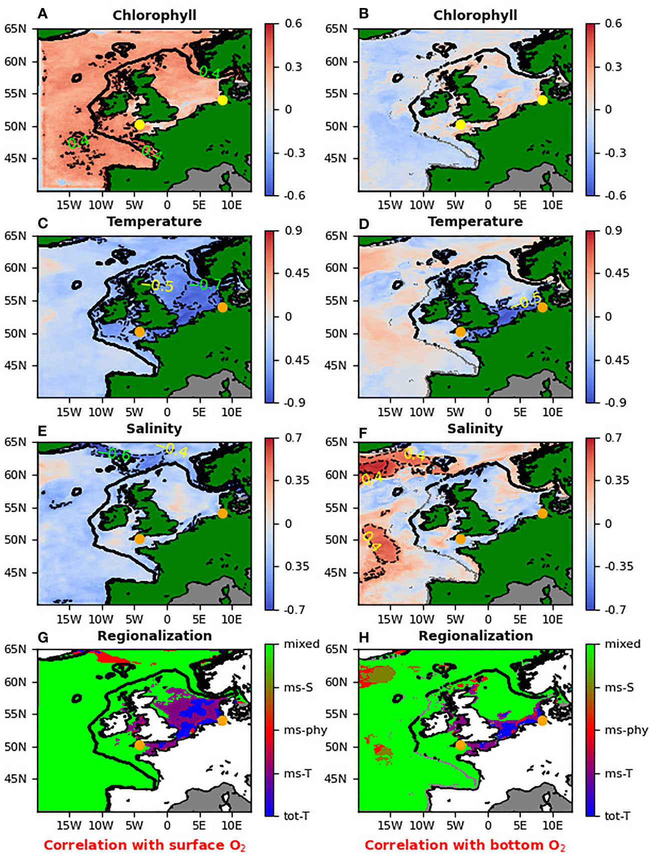
Figure 1 The top three rows (A-F) show for NWES the lagged Spearman correlation between the different ML model inputs (surface chlorophyll, SST, surface salinity anomalies) and the surface oxygen anomaly (left hand panels), or bottom oxygen anomaly (right hand panels). Both, the time-series of the ML model input variables and the oxygen are always correlated at the same location, but with a potentially non-zero time-lag, which at each location corresponded to the maximum absolute value of Spearman correlation (so the time-lags can change with the spatial location and can differ between input variables). The orange/yellow dots in all the panels show the L4 station in the English Channel and the GB location. The bottom plots (G, H, G for surface oxygen, H for bottom oxygen) show regionalization of the NWES based on correlations from the upper three panels. The different colors describe regions where oxygen is controlled by different variables: dominantly controlled by SST (“tot-T”, blue), mostly controlled by SST (“ms-T”, purple), mostly controlled by the surface salinity (“ms-S”, beige), controlled by both surface salinity and SST (“ms-phy”, red) and region where surface chlorophyll plays comparable role with SST and/or salinity (“mixed”, lime).

2.4.1 The L4 observing station

The L4 station is part of the Western Channel Observatory (WCO, https://www.westernchannelobservatory.org.uk/) and SmartSound Plymouth (https://www.smartsoundplymouth.co.uk/), based at 50m deep location (see Figure 2) about 13km from the Plymouth Sound area in the English Channel. The L4 location (50.25°N, 4.217°W) is highly biologically productive with seasonally stratified dynamics (Pingree and Griffiths (1978)), significantly impacted by the outflow of the nearby Tamar and Plym rivers. The oxygen dynamics at L4 shows a high degree of complexity, with comparable impact of biology and physics on the oxygen (see Figure 1). WCO, operated by Plymouth Marine Laboratory, runs at the L4 station one of the longest observational time-series (since 1988, Harris (2010)), delivering data typically with an average 7-10 day sampling frequency for physical ocean variables (temperature, salinity), biogeochemistry (e.g., chlorophyll, phytoplankton carbon, nutrients, oxygen, benthic data) and bio-optical data (e.g., PAR). As part of SmartSound Plymouth, the area near L4 station is continuously observed by other platforms (e.g., E1 buoy, vessels), and was also explored by the first fully autonomous glider bloom-tracking mission (Ford et al. (2022)).

FIGURE 2

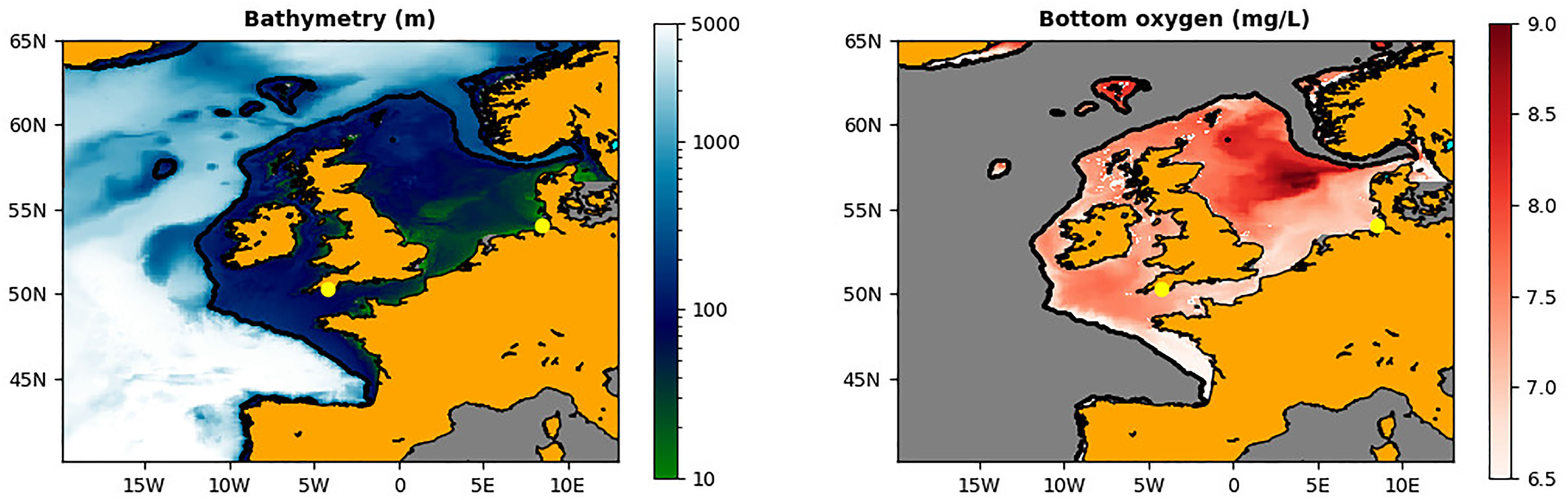
Figure 2 The left hand panel shows the bathymetry (in m) of the NWES for the AMM7 domain of the bi-decadal Met Office reanalysis. The right-hand panel shows the bottom oxygen concentrations (mg/L) for the NWES (the rest is masked), calculated from the 1998-2020 reanalysis data using the OSPAR methodology: the values represent the mean of the lowest quartile of the sea bottom oxygen during the stratified season between July and October (https://oap.ospar.org/en/). The L4 and GB locations are marked by the yellow dots.

The reanalysis data were extracted at the nearest model AMM7 domain grid cell to L4, the atmospheric forcing data were interpolated to the model grid location, whilst the riverine discharge data were taken from the area of 30km radius around the L4 location. Similar data processing methodology was used also at the GB location. Despite of slight mismatch in the locations and the major difference in spatial resolution, the temperature and oxygen variables agree very well between the Met Office reanalysis and the L4 observations (Figure 3 and Figure S3 of SI), however there is much less agreement in the total chlorophyll (Figure S4 of SI). This can be partly due to small-scale chlorophyll variability (e.g. Ford et al. (2022)) missed by the 7km resolution of the reanalysis data, but also partly due to differences between the L4 fluorescence-based chlorophyll measurements and the assimilated satellite chlorophyll, derived from the optical measurements (for more comparisons see also Skákala et al. (2018)).

FIGURE 3

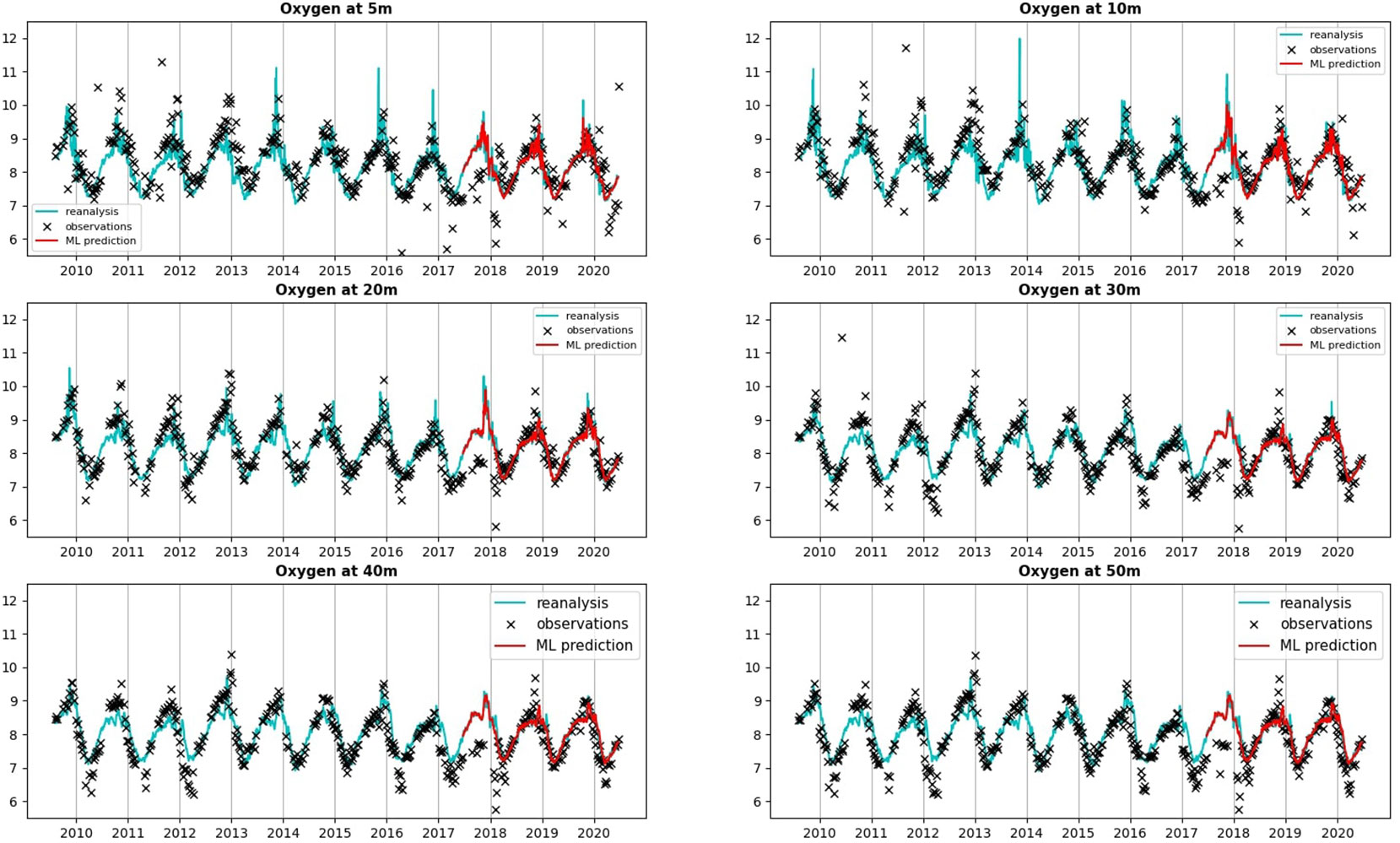
Figure 3 Comparing the oxygen total (climatology+anomaly) concentrations (in mg/L) at L4 between the reanalysis providing the training/validation/test data and the L4 observations. For completeness we show also the values predicted by a ML model (multilayer perceptron neural network) for the last 3 years of the time-series (2018-2020), which correspond to the test data. The ML model however predicted only the oxygen anomalies, which were added here to the L4 oxygen daily climatology known from the Met Office reanalysis. The oxygen concentrations are compared at a range of depths, excluding the surface values, since at the surface the L4 observations were largely missing. To show the limited oxygen range on the y-axes of the different panels, few observational outliers have been removed.

2.4.2 The German Bight (GB) location

Another location included in our study is in German Bight (54.067 °N, 8.444 °E). GB is a shallow section in the southeast of the North Sea, ranging from the coastline of Netherlands to the Danish coastal waters. It is an intertidal zone, near the substantial river deltas and estuaries (e.g., Elbe estuary). It is widely regarded as one of the most hypoxic zones in the North Sea, at risk of agricultural runoff and eutrophication (Brasse et al. (2002); Topcu and Brockmann (2015); Große et al. (2017); Brockmann et al. (2018)). The location selected for this study was 10m deep and very well mixed. It should be noted that in the 1998-2020 reanalysis used in this study there was no direct evidence of hypoxia (oxygen< 2mg/L) at the GB location (the bottom oxygen concentrations were always above 7 mg/L), and the oxygen was mainly driven by the SST (air-sea gas exchange, see Figure 1). This is likely a consequence of the data resolution (7km and 1 day), but model inadequacy in representing some of the processes leading to hypoxia cannot be ruled out (e.g., Oschlies et al. (2018)). Finally, due to the mixing and the shallow bathymetry, it is not very surprising that the SST turned out to be at the GB location also a good predictor of the bottom oxygen (Figure 1).

2.5 ML models

To guarantee that our analyses are robust, in this study we trained three separate ML models (Gaussian Process emulator, Long Short-Term Memory (LSTM) Neural Network and a standard Multilayer Perceptron (MLP) Neural Network), which belong to two highly expressive classes of supervised learning algorithms, Gaussian Processes and Deep Neural Networks (DNNs). ML models such as these are well suited to problems with multiple interactions between inputs and outputs, because they are able to model complex non-linear relationships between variables. Their straightforward architecture makes MLPs an effective baseline model, while LSTM-based models are specifically designed to identify dependencies in time series data. The three models are described in the following sections.

2.5.1 Gaussian process (GP) emulator and GP-based feature sensitivity analysis

As a robust non-parametric Bayesian inference framework, Gaussian Process (GP, Williams and Rasmussen (2006)) is a generalization of multivariate Gaussian distribution, such that any finite collection of the variables follows joint Gaussian distribution. GP can capture complex relationships between the model’s input and (noisy) output data. As with Gaussian distributions, the mean and covariance functions can completely describe a GP. Their parameters together with other model parameters, such as the measurement noise, are collectively called hyperparameters, and all of these can be learned from the training data. GP has been used for variety of applications, for instance, Bayesian optimization (Binois and Wycoff (2022)), predictive control (Kocijan et al. (2004)) and Bayesian filtering (Ko and Fox (2009)), among others. In this work we follow Williams and Rasmussen (2006) and use the squared exponential kernel with automatic relevance determination (SE-ARD) function to represent the covariances in the GP model.

Variance-based methods of probabilistic sensitivity analysis (Saltelli et al. (2000)) provide an efficient way to quantify the sensitivity of the GP model output to the GP model individual inputs through the total effect index. In this work, we follow the Bayesian approach of Oakley and O’Hagan (2004) to compute the total effect index.

2.5.2 Long short-term memory neural network emulator

Artificial neural networks (NN, e.g. Gurney (2018)) are models originally inspired by biological brains, constituted of interconnected and mutually communicating sets of nodes called neurons. Long Short-Term Memory (LSTM) networks are a type of neural network specifically designed to operate on time series. An LSTM cell replaces the standard neuron with a more complex set of operations, controlling how much information from the input at each time point is retained and how much is discarded (Hochreiter and Schmidhuber (1997)). This structure allows LSTMs to retain relevant information from previous time points for use in predicting the final output. As with a standard artificial neural network, an LSTM can be trained to predict an output, or set of outputs, given an input time series as a vector.

For this case, models were constructed using the Keras library (with TensorFlow backend) with the number of LSTM layers matching the number of input variables, where each input sequence is fed separately through an LSTM layer before the outputs are concatenated and connected to a fully connected output layer with size 50 (one output for each vertical layer). LSTM layers consist of a number of LSTM cells equal to the length of the input vector (i.e., the number of time steps). Models were trained for 20 epochs (sufficient to reach convergence) using the Adam optimizer and RMSE as a loss function.

2.5.3 Multilayer perceptron neural network emulator

We have also trained a simple Multilayer Perceptron (MLP) neural network (NN) model using the Python TensorFlow library. The MLP NN model had three hidden layers and the number of neurons in each hidden layer was set to scale as ten times the number of model inputs. Before the model was trained, we applied PCA and reduced the number of inputs by 30-50% (depending on the exact inputs). Similarly to the LSTM NN, the MLP NN model used the Adam optimizer and RMSE as a loss function. The model was typically trained on 15 epochs (sufficient to reach convergence).

2.6 ML forecasting

It should be noted that we trained our models to do both, predict the oxygen anomalies at a simultaneous time to (some of) the observational inputs and to forecast the oxygen anomalies into the future. To forecast the oxygen into the future, we have trained the ML model separately for each forecast lead time using the same ML model design and hyperparameters, with the only difference that the observed inputs were time-shifted from the predicted outputs by the forecast lead time.

3 Results and discussion

3.1 The controls over oxygen on the NWES

We used the 23 year reanalysis data to identify the key drivers behind the surface and bottom oxygen anomalies across the whole NWES (Figure 1). The impact of each driver was estimated based on lagged absolute Spearman correlation, where the correlation analysis was run separately at each location through a (-40 days to +40 days) interval of time-lags between the oxygen time-series and the time-series of the ML input variable (SST, surface chlorophyll, surface salinity). The overall lagged-Spearman correlation between the oxygen and the ML input variable, shown in Figure 1, then, separately for each location and input variable, corresponds to the time-lag that gave the largest absolute correlation value.

Figure 1 demonstrates that the surface observations for temperature, chlorophyll and salinity are good predictors for surface oxygen anomalies, but do not have strong relationship to the bottom oxygen. The exception are the areas mostly in the southern North Sea, which have very shallow bathymetry ($⪅$ 20m) and are well mixed. We can also see (Figure 1) that the physical variables (especially the SST) have stronger control over the oxygen concentrations than the biological variables (chlorophyll) and in some areas the oxygen anomalies can be predicted solely from their values. The regionalization shown in the bottom panels of Figure 1 shows that the surface oxygen anomalies in the south of North Sea are either “fully” (absolute lagged-Spearman correlation > 0.75), or “mostly” (absolute lagged-Spearman correlation > 0.5 and at least twice as large as the absolute lagged-correlation of the other variables) controlled by the SST anomalies.

The bottom oxygen anomalies are also controlled by the SST, but on a smaller portion of the domain, with shallow bathymetry. Except of some very limited sections of the NWES where salinity (“mostly”, in the same sense than for SST) controls the bottom oxygen anomalies, the rest of the domain (called “mixed”) is represented by much more complex dynamics where both biology and physics play a comparable role. The “mixed” domain was defined by either (i) the absolute values of lagged-correlation of all three (SST, salinity, chlorophyll) variables being lower than 0.5, or by (ii) the absolute lagged-correlation of none of the physical variables being twice as large as the absolute lagged-correlation of chlorophyll.

3.2 The GB location

The GB location falls in the region where oxygen anomalies are dominantly controlled by the SST anomalies (Figure 1). The same is shown by Figure 4 (and Figure S5 of SI), demonstrating the strong linear lagged-relationship between the surface oxygen anomaly and the SST anomaly. It is then not surprising that training a ML model (at GB location only MLP NN model was used, the other ML models were used only at L4 location, where the emulation is more complex) using only the SST inputs does a very good job in predicting the oxygen anomaly (Figure 5). Figure 4 in fact suggests that a simple linear interpolation model might be sufficient for the oxygen anomaly prediction, but we have observed that the linear model considerably underperformed compared to the MLP NN model from Figure 5, i.e., it had RMSE over 50% larger than MLP NN (not shown here).

FIGURE 4

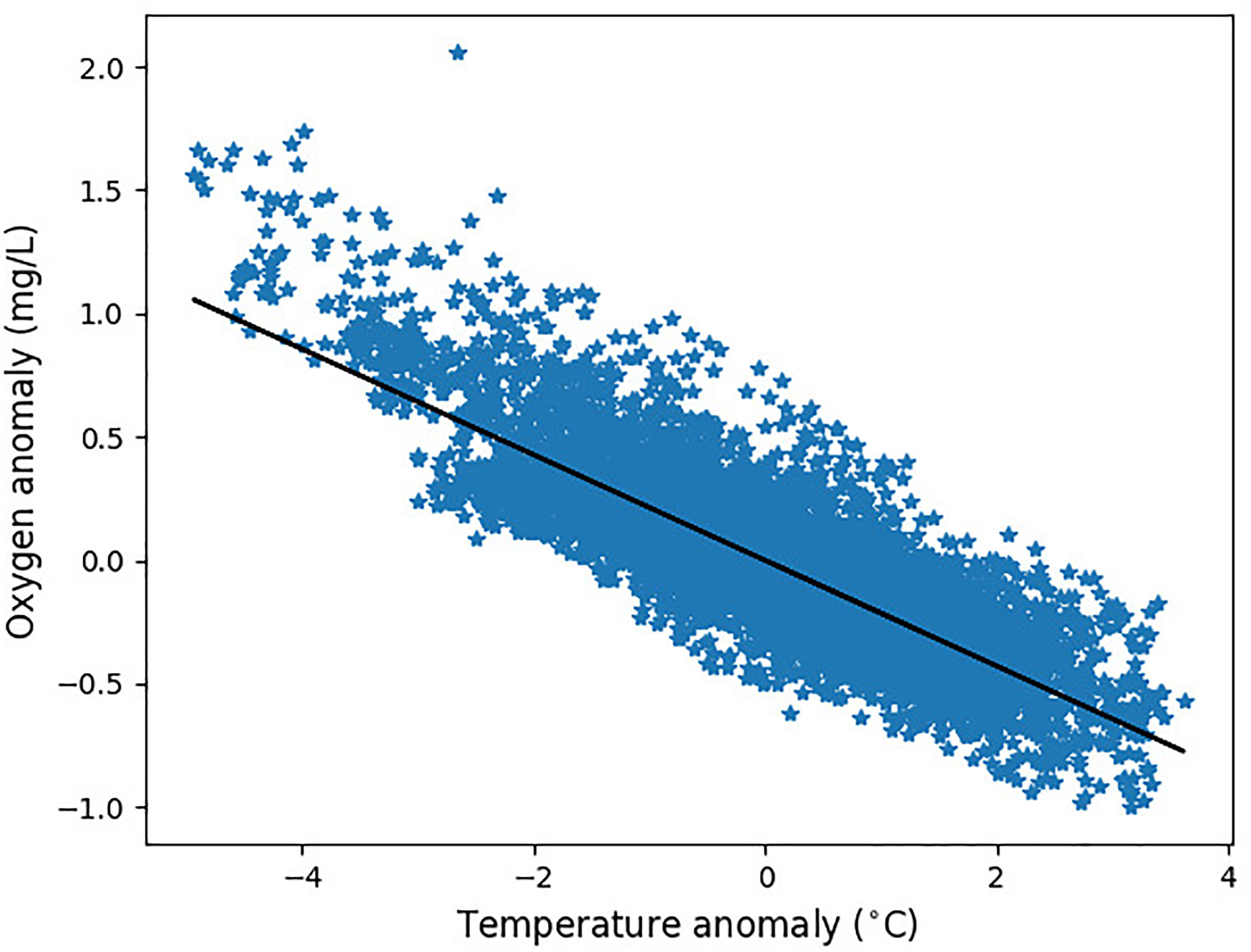
Figure 4 The relationship between the SST anomaly and oxygen anomaly (lagging on SST by 5 days) at the GB location. The Pearson correlation describing the linear relationship is R=-0.83.

FIGURE 5

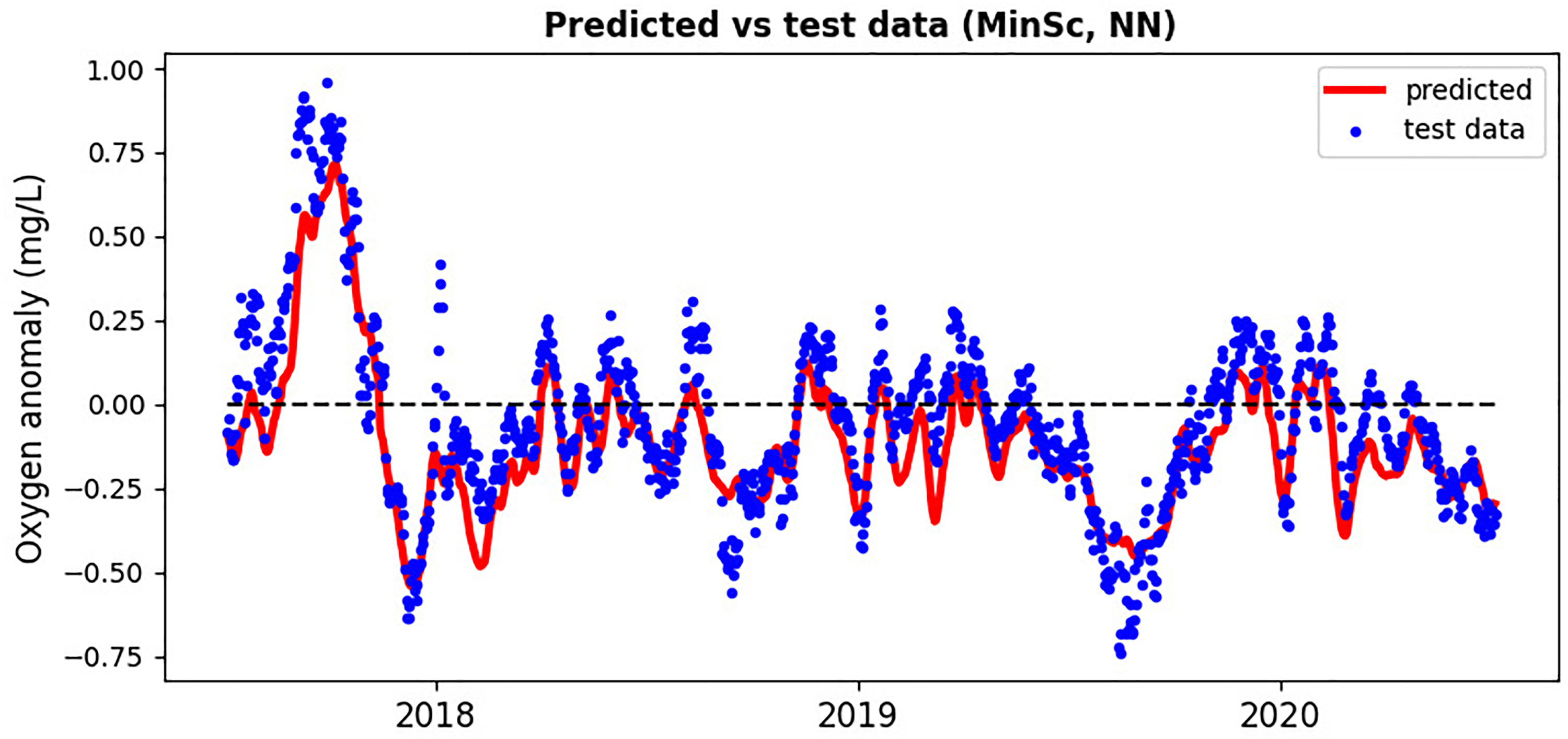
Figure 5 Neural network based on SST inputs predicting the surface oxygen anomaly at the GB location compared with the test data-set from 2018-2020.

Figure 6 demonstrates the MLP NN model capacity to forecast oxygen anomalies into the future. This is particularly important for the hypoxia warnings, as they need to be provided sufficient time in advance. Figure 6 shows that the model skill is broadly constant with depth (high degree of mixing in a 10m water-column) and the Pearson correlation drops from well over R=0.9 to about R=0.6 at the forecast lead time of about 17 days, with RMSE increasing on the same time-scale by about 50%. The long lead-time of this forecast can be understood from the long GB oxygen auto-correlation time-scales, that correspond to the relatively slow dynamics of the SST anomalies (Figure S6 of SI).

FIGURE 6

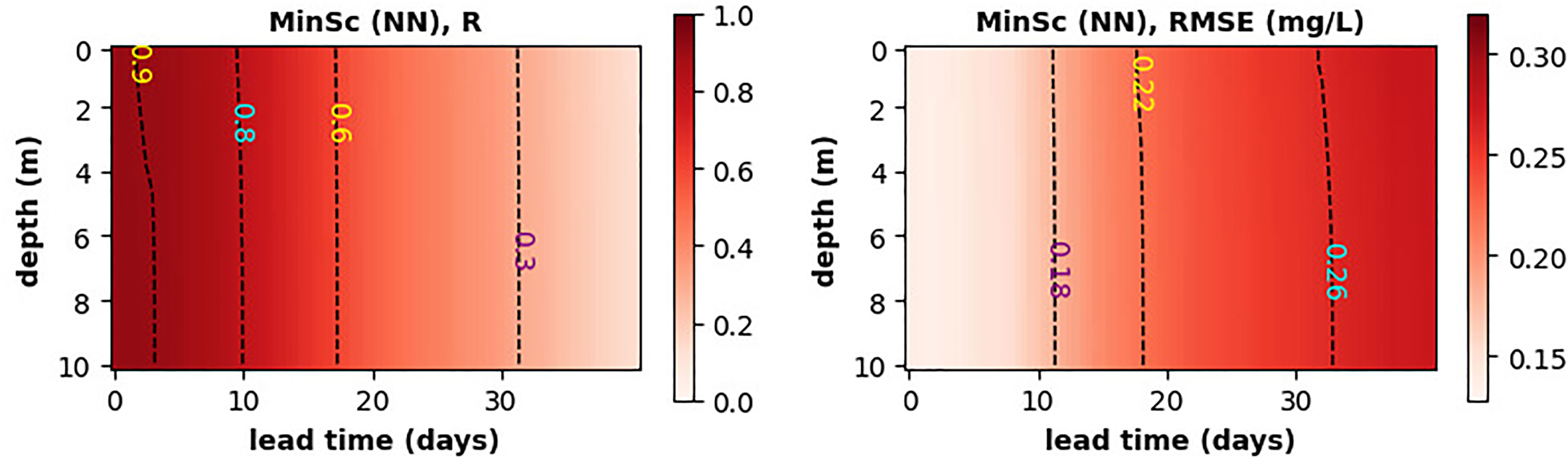
Figure 6 The skill of MLP NN model, measured by the Pearson correlation (left panel) and RMSE (right panel), to forecast oxygen anomaly across the full water-column at the GB location. The neural network uses as inputs only SST.

As mentioned in the Methods, the neural network did not predict oxygen anomaly in Figures 5, 6 from a single SST value, but from a whole time-interval of SST values ahead of the predicted oxygen. In fact, the left-hand panel of Figure 7 shows that for the ML model to perform optimally, we should include into the inputs the SST data on a time-interval with length of at least two weeks. To be able to do prediction from such long time-interval of inputs, one always needs to have available SST data on a large number of successive days. Such availability is rare with satellite SST data with a daily time-resolution, as satellite SST from a specific location will usually have temporal gaps in the data. It is thus important to estimate how the ML model skill depends on the time-resolution of the SST inputs. Figure 7, the right-hand panel, demonstrates that the skill of the ML model did not substantially change when the SST inputs were low-pass filtered on a time-scale of up to 30 days. This suggests that the daily time-resolution of satellite SST is not necessary, i.e., the MLP NN model using satellite SST time-series with much coarser time-resolution (even > week) would perform similarly to the one using daily data. This is important, since the coarser the resolution, the more we are allowed to fill the data gaps with interpolation. These results demonstrate that the oxygen prediction can be easily performed in realistic situations with widely available observational products.

FIGURE 7

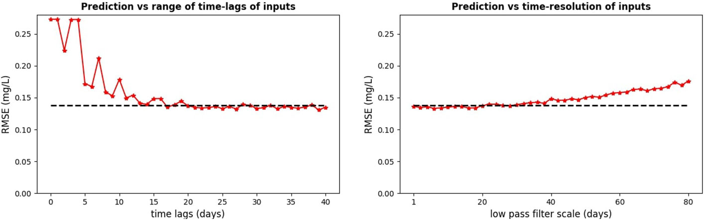
Figure 7 The necessary time-lags in the SST inputs (left-hand panel) and the required time-resolution of the input data (right-hand panel). The RMSE values on the y-axis of the left-hand panel are shown for simulations using in their inputs always the full range of time-lags from the zero time-lag to maximum time-lags corresponding to the values on the x-axis. The analysis is for MLP NN model at the GB location.

The relatively stable GB oxygen anomaly time-series with long auto-correlation time-scales (e.g., Figure 5 and Figure S6 of SI) are probably an artefact of the relatively coarse spatio-temporal resolution of the Met Office reanalysis. So is likely the absence of hypoxia in the GB reanalysis: it is known that due to high level of mixing and the shallow bathymetry in the GB area, the hypoxic events are relatively short-lived compared to much more stratified waters [Topcu and Brockmann (2015)]. It is therefore expected that on a finer spatio-temporal resolution scale we would see much greater extremes in the oxygen anomalies, and these will be inherently predictable only when riverine discharge and chlorophyll variables were added to the ML model inputs. Unfortunately, this hypothesis remains to be tested, as sufficient amount of high-resolution data, needed to train the ML models, is not available for the GB. As for the Met Office reanalysis, adding chlorophyll, or riverine data to ML model inputs did not further improve the ML model skill, e.g., it did not capture better some of the extremes of the test data missed by the ML model (a positive extreme in the Summer 2018, and negative extremes in the Winter 2019 and 2020, shown in Figure 5).

3.3 L4 location

Whilst SST anomalies have similar auto-correlation lengthscales between L4 and GB locations (Figures S6, S7 of SI), unlike GB, the L4 oxygen anomalies are better correlated with chlorophyll (Figure S8 of SI) and have shorter auto-correlation lengthscales than SST (Figure S7 of SI). This means, at L4, biological processes play an important role in the predicted oxygen (see also Figure 1). Furthermore, the L4 location is highly seasonally stratified and the surface values are effectively decoupled from the values near the sea bottom. This makes the problem of predicting oxygen anomalies much more non-trivial, but also more interesting.

3.3.1 The sensitivity of oxygen anomalies to the observed variables

The three ML models were used to investigate the sensitivity of the predicted oxygen anomalies to the atmospheric, riverine inputs as well as the SST, surface salinity and surface chlorophyll. In this analysis only the inputs from the MinSc case were considered.

The sensitivity results were consistent between the three ML models, which indicates that the results are robust. The most systematic analysis was performed using the GP emulator and is shown in Figure 8. The ranking based on the total effect index shows that for the near-surface oxygen, the PFT chlorophyll, SST and surface salinity are the most important inputs, with additional impacts from phosphorus and ammonium riverine inputs (Figure 8). In the deeper layers the ranking does not dramatically change, however the impact of PFT chlorophyll is significantly diminished, whilst the impact of riverine phosphorus and ammonium load remains similar to what it was near the surface. These results are consistent with what has been anticipated based on Table 1, however some specific details need explanation, i.e., the high ranking of phosphorus riverine discharge indicates that phytoplankton growth in the model is phosphorus-limited. This contradicts the established knowledge that productivity at L4 is mostly nitrogen-limited (Smyth et al. (2010)). We suspect this discrepancy is an artefact of the emulated ERSEM model, which overestimates nitrates at L4 (Skákala et al. (2018)) and fails to capture the observed nitrogen-limitation of the phytoplankton growth.

FIGURE 8

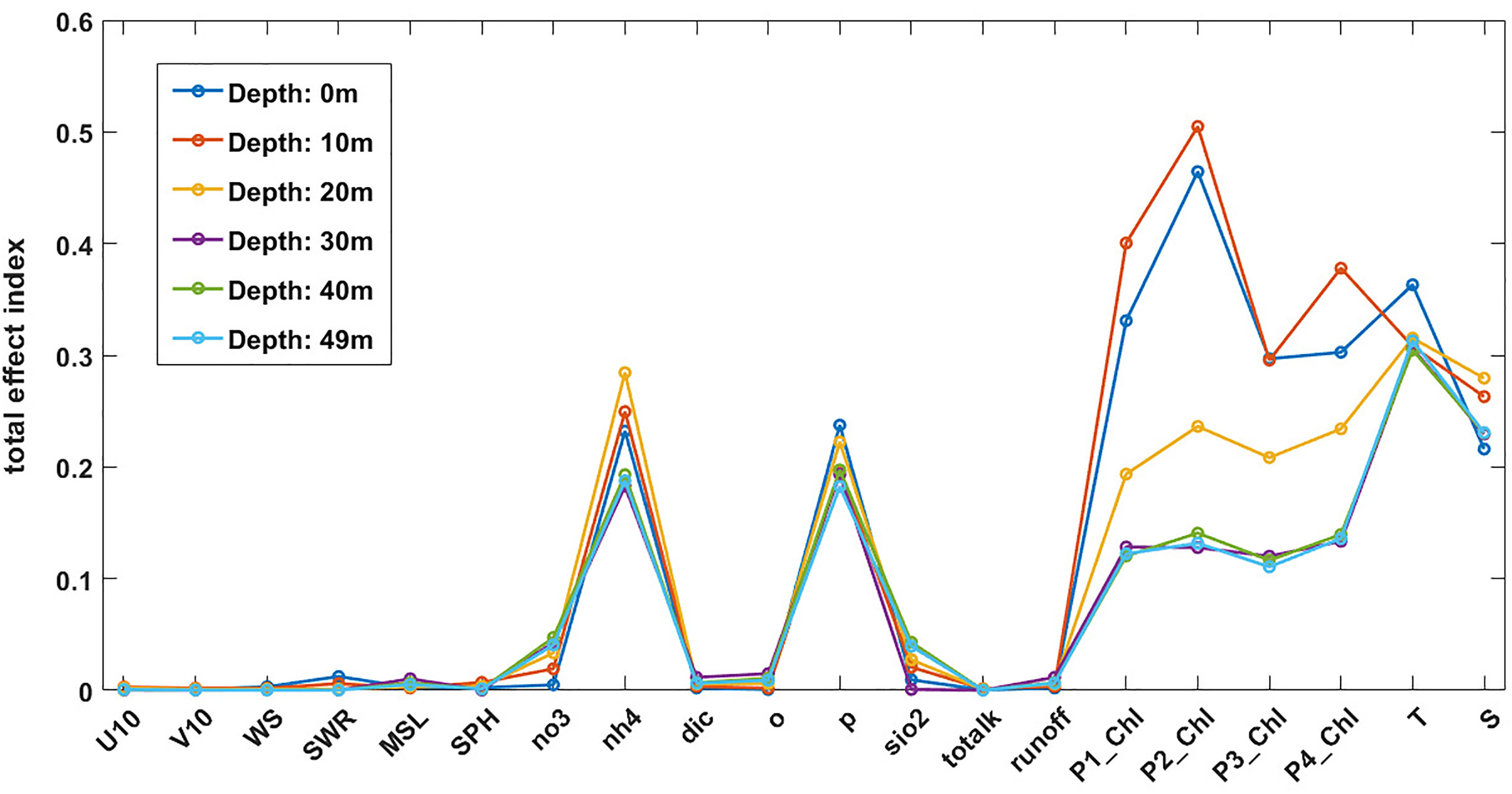
Figure 8 Total effect indexes for the full range of ML model inputs from the MinSc case at the L4 location. The abbreviations are: “U10”: zonal wind at 10m, “V10”: meridional wind at 10m, “WS”: total wind speed, “SWR”: incoming short-wave radiation, “MSL”: mean sea level pressure, “SPH”: specific humidity, “no3”: riverine nitrate input, “nh4”: riverine ammonium input, “dic”: riverine dissolved inorganic carbon input, “o”: riverine oxygen input, “p”: riverine phosphorus input, “sio2”: riverine silicate input, “totalk”: riverine total alkalinity input, “runoff”: the freshwater runoff by the river, “P1_Chl”: diatoms chlorophyll, “P2_Chl”: nanophytoplankton chlorophyll, “P3_Chl”: picophytoplankton chlorophyll, “P4_Chl”:dinoflaggelates chlorophyll (all on the surface), “T”: sea surface temperature, “S”: surface salinity. The different lines correspond to the predicted oxygen outputs at different depths (marked in the legend).

Based on other sensitivity tests performed with the MLP NN emulator (not shown here), the MLP NN model at L4 was run in the MinSc case only with total chlorophyll (sum of PFT chlorophyll), SST and riverine phosphorus inputs. The LSTM NN model used the same features as the MLP NN model (based on its own analysis), with additional inputs for riverine ammonia discharge and incoming short-wave radiation.

3.3.2 The prediction of oxygen from the relevant inputs

The three ML models considered in this study were highly variable in their skill, depending on the type of scenario, the depth of the predicted oxygen anomaly, and the forecast lead time. The detailed comparison of the model skill is for the three scenarios (MinSc, MedSc, MaxSc) shown in Figures S9-S11 of the SI. The conclusion drawn from this analysis is that there is no best-performing ML model among the three: the most appropriate choice of the ML model depends on the specific scenario, vertical depth and the forecast lead time. Furthermore, it should be noted, that greater model complexity does not necessarily imply better performance. For example, the GP model performed worse for the MedSc and MaxSc cases than for the MinSc case, since as a nonparametric model it is more prone to overfitting, and also requires more data for larger input dimensions to train its hyperparameters. However, despite of the many differences in the performance of the three ML models, all the models led broadly to similar conclusions. This is very encouraging, as it indicates that those conclusions are robust. Hence, the results presented here are based on the MLP NN model, but similarly, they could have been based on any of the other two ML models (GP, LSTM NN).

To predict sub-surface oxygen in the stratified waters, the ML model needs to carry information about the vertical profiles of the physical and biogeochemical variables. In the MinSc case it is hard for the ML model to deduce those profiles, except for trying to predict them from the atmospheric forcing (e.g. the wind stress data, see Table 1). Figures 8, 9 (left-hand panel) demonstrate that the atmospheric forcing data are of minimal use, and the MLP NN model in the MinSc case fails to predict well the sub-surface (>10m depth) oxygen anomalies. However, providing physical profiles by adding sub-surface temperature anomalies to the inputs (MedSc, middle panel of Figure 9) leads to significant improvement in the sub-surface oxygen anomalies. This is further improved when the sub-surface chlorophyll anomalies are added to the model inputs (MaxSc, right-hand panel of Figure 9). Finally, Figure 9 also demonstrates that the MLP NN model maintains most of its prediction skill within the 5 day (MinSc) or 7-10 day (MedSc,MaxSc) forecast lead time.

FIGURE 9

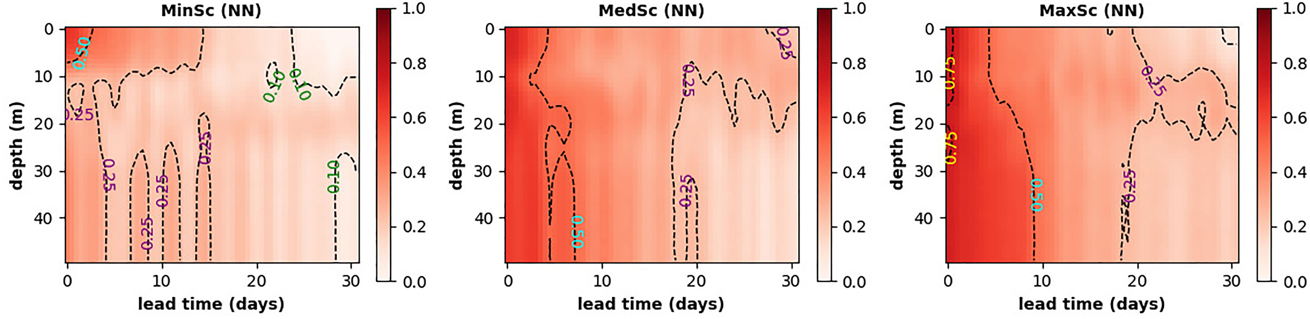
Figure 9 The MLP NN model forecast skill measured by the Pearson correlation shown for the full range of depths at L4 (y-axis) vs the forecast lead time (on the x-axis). The three panels are the three scenarios explored in this study: using only surface chlorophyll and temperature data (MinSC, left-hand panel), using also sub-surface temperature data (MedSC, middle panel) and using both temperature and chlorophyll sub-surface data (MaxSC, right-hand panel).

The results for MedSc and MaxSc (Figure 9) are based on inputs for temperature (MedSc) and also chlorophyll (MaxSc) supplied for all 50 model vertical grid cells. However, it is unrealistic to expect that measurements can be made with such resolution across the whole water column unless they are done by an autonomous underwater vehicle, such as a glider. It is, therefore, essential to determine at how many sub-surface grid cells (on top of the existing surface inputs) one needs to provide the input information for temperature, or chlorophyll, to achieve a skilled prediction of the sub-surface oxygen anomaly. The answer is provided by Figure 10, showing that for the MLP NN model to perform well (everywhere R > 0.5 for MedSc and R > 0.6 for MaxSc) in predicting sub-surface oxygen anomalies in all 50 vertical grid cells, it is enough to provide temperature (MedSc), or temperature and chlorophyll (MaxSc), in one single additional sub-surface cell at the 25m depth. This typically lies beneath the mixed layer, at the L4 location, during the stratified period (e.g., see Powley et al. (2020)). When inputs in some other vertical cells are added to the model, we can further improve its performance, but the gain is relatively small compared to the addition of the single vertical cell at 25m. This is encouraging, as collecting observations at the surface and at one another deeper location is a realistic prospect.

FIGURE 10

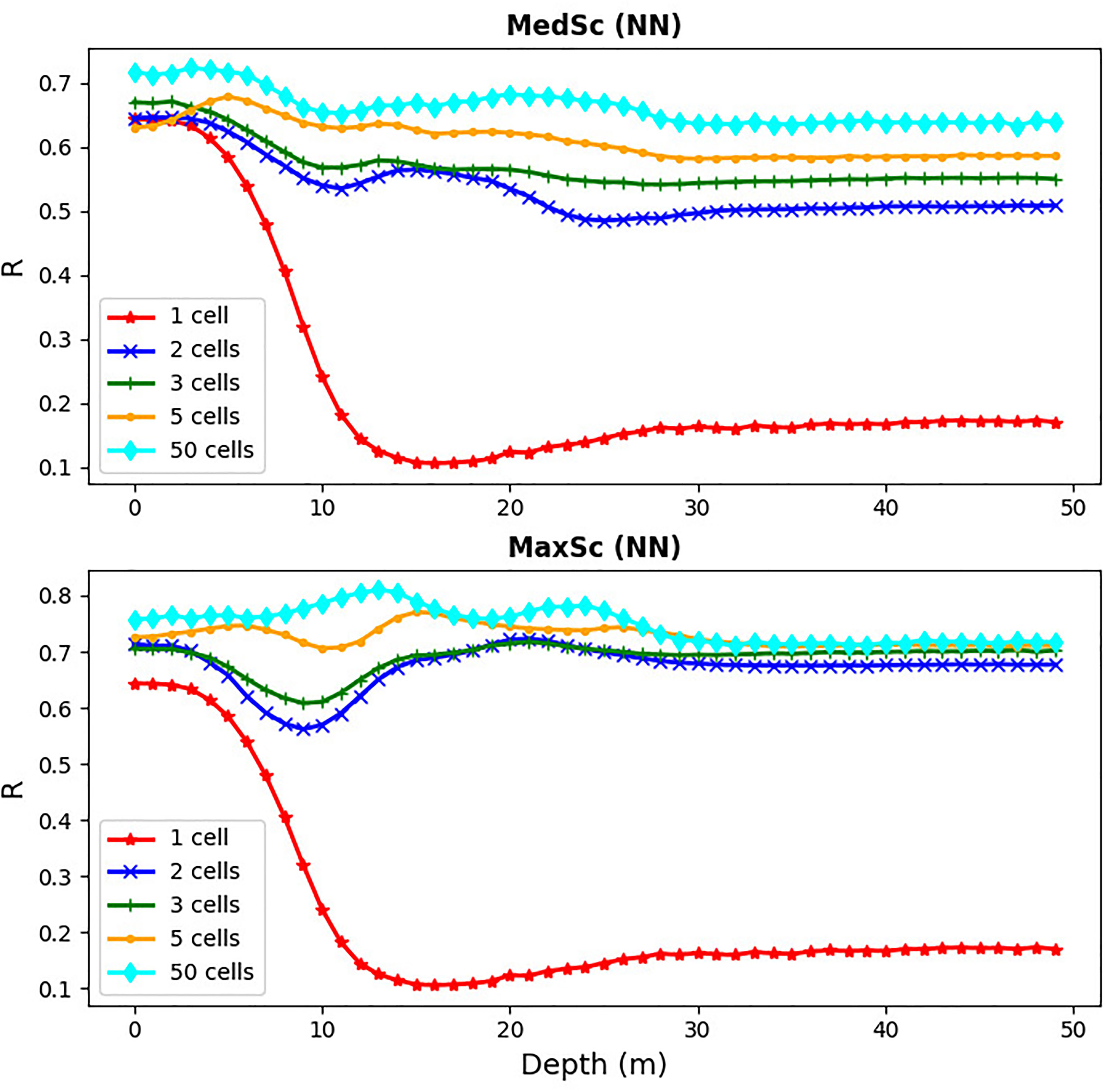
Figure 10 The skill of the MLP NN model (Pearson correlation) as a function of depth at the L4 location (x-axis) for different numbers of inputs in the vertical dimension: inputs at two, three, five and all fifty vertical cells in the water-column. The three, five and fifty vertical cells were always selected to have one cell located on the ocean surface, one on the sea bottom and the other(s) always regularly spaced in between (e.g., for three cells the cells were selected at the 0m, 25m and 50m depths). In case of one cell, the cell was placed at the surface, for two cells they were placed at the surface and the 25m depth (the middle of the water column). The upper panel is the MedSc case and the bottom panel the MaxSc case.

Similarly to the GB location, it is hard to realistically expect that the observations at the L4 station can be supplied with a daily resolution for a successive number of days, in order to provide the time-lagged inputs into the ML model. Figure 11 is thus an analogue of Figure 7, and shows the skill of the MLP NN model when the time-resolution of the model inputs is coarsened through applying a low-pass filter. Similarly to Figure 7, Figure 11 demonstrates that the model skill is mostly preserved when the time-resolution is coarsened by up to 30 days. This is again good news: such smoothed SST, or chlorophyll, time-series can be typically estimated from the daily observational products, despite of their many missing values. Furthermore, it should be noted that in Figure 11, low time-resolution ML model inputs were used to predict high time-resolution (daily) oxygen anomalies; if the predicted oxygen anomalies were taken on the same coarse resolution time-scale as the ML model inputs, the model skill would be much better (see Figure S12 of SI).

FIGURE 11

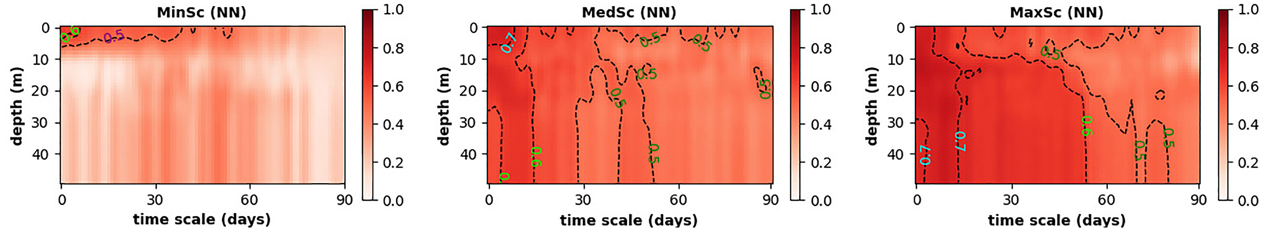
Figure 11 The dependence of the MLP NN model (Pearson correlation) skill across the full range of L4 depths (y-axis) on the time-resolution of the data (the time-scale of the low-pass filter, x-axis). Similarly to Figure 9, the different panels show the different scenarios explored here.

Finally, we have attempted to directly apply the ML models trained on the reanalysis data to the total chlorophyll and SST anomalies derived from the observations at the L4 station, and compare the model outputs to the anomaly derived from the L4 observed oxygen. To overcome the limitation of the L4 observational sampling frequency of ~10 days, we had to heavily interpolate the missing observational values, and estimate the L4 observational anomalies based on the (smoothed) climatology of the interpolated L4 data. Unfortunately, it turned out that the ML models performed poorly on the L4 interpolated anomaly inputs (not shown here), when validated by the L4 oxygen anomaly estimates. There are a number of possible reasons for why this has happened:

(i) While the temperature and oxygen L4 observations compare very well with the reanalysis (Figures 3, Figure S3 of SI), there is a clear mismatch between the total surface chlorophyll L4 observations and the reanalysis, based on assimilating the satellite OC chlorophyll data (Figure S4 of SI). This discrepancy in the chlorophyll values can be easily caused by the different spatial and temporal resolutions of the two products, since, unlike temperature and oxygen, chlorophyll has at L4 large small-scale variability (e.g., see Figure S2 of SI). The instantaneous L4 chlorophyll measurements, with their sparse sampling frequency (~10 days), might be then highly non-representative of the biological productivity driving oxygen concentrations at the L4 location. The heavily interpolated L4 chlorophyll observations might be therefore a poor predictor of oxygen.

(ii) With the limited number of raw L4 observations, it is highly non-trivial to derive from the total values of the observed variables their anomalies. For example, applying the anomaly calculation procedure to the observed L4 oxygen reduced the correlation between the reanalysis and the L4 observations from R=0.68 for the total oxygen values (Figure 3) to R<0.2 between the oxygen anomalies. This means the anomaly estimation procedure presumably introduced large biases to the L4 oxygen anomaly data, both due to lack of sufficient number of long-term L4 oxygen observations and potentially also due to some noisy observational values (especially around the year 2017, see Figure 3).

4 Conclusions

We explored ways how to build computationally cheap and efficient machine learning (ML) emulators to replace a computationally expensive complex physical-biogeochemical model. These ML emulators can provide essential components within future digital twin applications. In particular, we build ML emulators to predict oxygen anomalies, including hypoxia, at the selected locations in the North Sea and in the western English Channel. The stakeholder applications we had in mind are: (i) monitoring the risk of hypoxia by the aquaculture farmers in the German Bight region of the North Sea, and (ii) expanding the observed data into unobserved variables at the L4 coastal monitoring station in the western English Channel.

We have shown that complex models can be replaced with computationally cheap ML surrogates that are capable to successfully predict simulated oxygen anomalies with relatively modest requirements on the ML model inputs. We have identified the observable variables with the highest impact on the oxygen anomalies, throughout the whole water-column and in different types of environments (mixed, stratified). For the near-surface oxygen, the most essential observable variables are the SST, surface chlorophyll and some specific riverine discharge data. We have demonstrated that to predict sub-surface oxygen across the stratified water-column it is often sufficient to measure temperature at a single location (in addition to the surface), that is typically beneath the mixed layer (25m at L4). Similarly, for the ML model, it is sufficient to provide the surface observation inputs with a coarse temporal resolution (e.g., weekly). These can be always supplied, with the required quality, by the satellite data with interpolated observational gaps.

There are some issues that need addressing in the future, e.g. to develop successful digital twins for high resolution applications, we might need to adapt the observational sampling strategies to the needs of the ML models. However, as discussed before, this can be often done without a major increase in the observational cost. But improvements need to be done also on the modelling side, e.g., (i) we need to either increase the model resolution to better approximate the scales of (most of) the digital twin applications, or we need to find ways how to downscale the model outputs, (ii) we also need to ensure that the dynamics relevant to the digital twin application is as well represented in the model, as possible.

Data availability statement

Publicly available datasets were analyzed in this study. This data can be found in CMEMS repository as NWSHELF_MULTIYEAR_BGC_004_011 (DOI: https://doi.org/10.48670/moi-00059) and NWSHELF_MULTIYEAR_PHY_004_009 (DOI: https://doi.org/10.48670/moi-00058).

Author contributions

JS authored the original project idea and prepared the data. KA-C, PM, JS, and KW developed the ML models and produced the results. JS led the manuscript writing, and all authors (KA-C, GL, PM, JS, and KW) substantially contributed to the manuscript with text and ideas. All authors contributed to the article and approved the submitted version.

Funding

This work was supported by the PML Research Grant REPLACing complEx biogeochemical models with machine learning (REPLACE) and by the NERC single center national capability programme – Climate Linked Atlantic Sector Science (NE/R015953/1).

Acknowledgments

The study was conducted using EU Copernicus Marine Service information; the reanalyses used were NWSHELF_MULTIYEAR_BGC_004_011 (DOI: https://doi.org/10.48670/moi-00059) and NWSHELF_MULTIYEAR−_PHY−_004_009 (DOI: https://doi.org/10.48670/−moi-00058). The atmospheric forcing data were obtained from the ERA5 product of The European Centre for Medium-Range Weather Forecasts (ECMWF, https://www.ecmwf.int/). The riverine data were prepared by Sonja van Leeuwen and Helen Powley as part of UK Shelf Seas Biogeochemistry programme (contract no. NE/K001876/1) of the NERC and the Department for Environment Food and Rural Affairs (DEFRA). We would like to thank Stefano Ciavatta and Jerry Blackford for the discussions and useful comments, as well as David Ford and Richard Renshaw for providing us with the reanalysis data and the data description.

Conflict of interest

The authors declare that the research was conducted in the absence of any commercial or financial relationships that could be construed as a potential conflict of interest.

Publisher’s note

All claims expressed in this article are solely those of the authors and do not necessarily represent those of their affiliated organizations, or those of the publisher, the editors and the reviewers. Any product that may be evaluated in this article, or claim that may be made by its manufacturer, is not guaranteed or endorsed by the publisher.

Supplementary material

The Supplementary Material for this article can be found online at: https://www.frontiersin.org/articles/10.3389/fmars.2023.1058837/full#supplementary-material

References

Artioli Y., Blackford J. C., Butenschön M., Holt J. T., Wakelin S. L., Thomas H., et al. (2012). The carbonate system in the north sea: Sensitivity and model validation. J. Mar. Syst. 102, 1–13. doi: 10.1016/j.jmarsys.2012.04.006

CrossRef Full Text | Google Scholar

Bannister R. (2017). A review of operational methods of variational and ensemble-variational data assimilation. Q. J. R. Meteorological Soc. 143, 607–633. doi: 10.1002/qj.2982

CrossRef Full Text | Google Scholar

Baretta J., Ebenhöh W., Ruardij P. (1995). The european regional seas ecosystem model, a complex marine ecosystem model. Netherlands J. Sea Res. 33, 233–246. doi: 10.1016/0077-7579(95)90047-0

CrossRef Full Text | Google Scholar

Baretta-Bekker J., Baretta J., Ebenhöh W. (1997). Microbial dynamics in the marine ecosystem model ersem ii with decoupled carbon assimilation and nutrient uptake. J. Sea Res. 38, 195–211. doi: 10.1016/S1385-1101(97)00052-X

CrossRef Full Text | Google Scholar

Binois M., Wycoff N. (2022). A survey on high-dimensional Gaussian process modeling with application to Bayesian optimization. ACM Transactions on Evolutionary Learning and Optimization 2(2), 1–26. doi: 10.1145/3545611

CrossRef Full Text | Google Scholar

Blackford J. (1997). An analysis of benthic biological dynamics in a north sea ecosystem model. J. Sea Res. 38, 213–230. doi: 10.1016/S1385-1101(97)00044-0

CrossRef Full Text | Google Scholar

Blair G. S. (2021). Digital twins of the natural environment. Patterns 2, 100359. doi: 10.1016/j.patter.2021.100359

PubMed Abstract | CrossRef Full Text | Google Scholar

Bostock J., McAndrew B., Richards R., Jauncey K., Telfer T., Lorenzen K., et al. (2010). Aquaculture: global status and trends. Philos. Trans. R. Soc. B: Biol. Sci. 365, 2897–2912. doi: 10.1098/rstb.2010.0170

CrossRef Full Text | Google Scholar

Brasse S., Nellen M., Seifert R., Michaelis W. (2002). The carbon dioxide system in the elbe estuary. Biogeochemistry 59, 25–40. doi: 10.1023/A:1015591717351

CrossRef Full Text | Google Scholar

Brenowitz N. D., Bretherton C. S. (2018). Prognostic validation of a neural network unified physics parameterization. Geophysical Res. Lett. 45, 6289–6298. doi: 10.1029/2018GL078510

CrossRef Full Text | Google Scholar

Brewin R. J., Ciavatta S., Sathyendranath S., Jackson T., Tilstone G., Curran K., et al. (2017). Uncertainty in ocean-color estimates of chlorophyll for phytoplankton groups. Front. Mar. Sci. 4, 104. doi: 10.3389/fmars.2017.00104

CrossRef Full Text | Google Scholar

Brockmann U., Topcu D., Schütt M., Leujak W. (2018). Eutrophication assessment in the transit area german bight (north sea) 2006–2014–stagnation and limitations. Mar. pollut. Bull. 136, 68–78. doi: 10.1016/j.marpolbul.2018.08.060

PubMed Abstract | CrossRef Full Text | Google Scholar

Bruggeman J., Bolding K. (2014). A general framework for aquatic biogeochemical models. Environ. Model. software 61, 249–265. doi: 10.1016/j.envsoft.2014.04.002

CrossRef Full Text | Google Scholar

Butenschön M., Clark J., Aldridge J. N., Allen J. I., Artioli Y., Blackford J., et al. (2016). Ersem 15.06: a generic model for marine biogeochemistry and the ecosystem dynamics of the lower trophic levels. Geoscientific Model. Dev. 9, 1293–1339. doi: 10.5194/gmd-9-1293-2016

CrossRef Full Text | Google Scholar

Davidson F., Alvera-Azcarate A., Barth A., Brassington G. B., Chassignet E. P., Clementi E., et al. (2019). Synergies in operational oceanography: the intrinsic need for sustained ocean observations. Front. Mar. Sci. 6, 450. doi: 10.3389/fmars.2019.00450

CrossRef Full Text | Google Scholar

De Mora L., Butenschön M., Allen J. (2016). The assessment of a global marine ecosystem model on the basis of emergent properties and ecosystem function: a case study with ersem. Geoscientific Model. Dev. 9, 59–76. doi: 10.5194/gmd-9-59-2016

CrossRef Full Text | Google Scholar

Diaz R. J., Rosenberg R. (2008). Spreading dead zones and consequences for marine ecosystems. science 321, 926–929. doi: 10.1126/science.1156401

PubMed Abstract | CrossRef Full Text | Google Scholar

Dohan K., Maximenko N. (2010). Monitoring ocean currents with satellite sensors. Oceanography 23, 94–103. doi: 10.5670/oceanog.2010.08

CrossRef Full Text | Google Scholar

Falkowski P. G., Algeo T., Codispoti L., Deutsch C., Emerson S., Hales B., et al. (2011). Ocean deoxygenation: past, present, and future. Eos Trans. Am. Geophysical Union 92, 409–410. doi: 10.1029/2011EO460001

CrossRef Full Text | Google Scholar

Flynn K. J., Torres R., Irigoien X., Blackford J. C. (2022). Plankton digital twins–a new research tool. Journal of Plankton Research. 44(6), 805–805. doi: 10.1093/plankt/fbac042

CrossRef Full Text | Google Scholar

Ford D., Grossberg S., Rinaldi G., Menon P., Palmer M., Skákala J., et al. (2022). A solution for autonomous, adaptive monitoring of coastal ocean ecosystems: integrating ocean robots and operational forecasts. Front. Mar. Sci., 9. doi: 10.3389/fmars.2022.1067174

CrossRef Full Text | Google Scholar

Ford D., Key S., McEwan R., Totterdell I., Gehlen M. (2018). Marine biogeochemical modelling and data assimilation for operational forecasting, reanalysis, and climate research. New Front. Operational Oceanogr, 625–652. doi: 10.17125/gov2018.ch22

CrossRef Full Text | Google Scholar

Franks P. J. (2002). Npz models of plankton dynamics: their construction, coupling to physics, and application. J. Oceanogr 58, 379–387. doi: 10.1023/A:1015874028196

CrossRef Full Text | Google Scholar

Geider R., MacIntyre H., Kana T. (1997). Dynamic model of phytoplankton growth and acclimation: responses of the balanced growth rate and the chlorophyll a: carbon ratio to light, nutrient-limitation and temperature. Mar. Ecol. Prog. Ser. 148, 187–200. doi: 10.3354/meps148187

CrossRef Full Text | Google Scholar

Giglio D., Lyubchich V., Mazloff M. R. (2018). Estimating oxygen in the southern ocean using argo temperature and salinity. J. Geophysical Research: Oceans 123, 4280–4297. doi: 10.1029/2017JC013404

CrossRef Full Text | Google Scholar

Good S. A., Martin M. J., Rayner N. A. (2013). En4: Quality controlled ocean temperature and salinity profiles and monthly objective analyses with uncertainty estimates. J. Geophysical Research: Oceans 118, 6704–6716. doi: 10.1002/2013JC009067

CrossRef Full Text | Google Scholar

Greenwood N., Parker E., Fernand L., Sivyer D., Weston K., Painting S., et al. (2010). Detection of low bottom water oxygen concentrations in the north sea; implications for monitoring and assessment of ecosystem health. Biogeosciences 7, 1357–1373. doi: 10.5194/bg-7-1357-2010

CrossRef Full Text | Google Scholar

Große F., Kreus M., Lenhart H.-J., Pätsch J., Pohlmann T. (2017). A novel modeling approach to quantify the influence of nitrogen inputs on the oxygen dynamics of the north sea. Front. Mar. Sci. 4, 383. doi: 10.3389/fmars.2017.00383

CrossRef Full Text | Google Scholar

Gurney K. (2018). An introduction to neural networks (CRC press).

Google Scholar

Harris R. (2010). The l4 time-series: the first 20 years. J. Plankton Res. 32, 577–583. doi: 10.1093/plankt/fbq021

CrossRef Full Text | Google Scholar

Heinze C., Gehlen M. (2013). Modeling ocean biogeochemical processes and the resulting tracer distributionsInternational geophysics Vol. 103 (Elsevier), 667–694.

Google Scholar

Helm K. P., Bindoff N. L., Church J. A. (2011). Observed decreases in oxygen content of the global ocean. Geophysical Res. Lett. 38(23). doi: 10.1029/2011GL049513

CrossRef Full Text | Google Scholar

Hemmings J., Challenor P. G., Yool A. (2015). Mechanistic site-based emulation of a global ocean biogeochemical model (medusa 1.0) for parametric analysis and calibration: an application of the marine model optimization testbed (marmot 1.1). Geoscientific Model. Dev. 8, 697–731. doi: 10.5194/gmd-8-697-2015

CrossRef Full Text | Google Scholar

Hochreiter S., Schmidhuber J. (1997). Long short-term memory. Neural Comput. 9, 1735–1780. doi: 10.1162/neco.1997.9.8.1735

PubMed Abstract | CrossRef Full Text | Google Scholar

Hooten M. B., Leeds W. B., Fiechter J., Wikle C. K. (2011). Assessing first-order emulator inference for physical parameters in nonlinear mechanistic models. J. Agricultural Biological Environ. Stat 16, 475–494.

Google Scholar

Ito T., Minobe S., Long M. C., Deutsch C. (2017). Upper ocean o2 trends: 1958–2015. Geophysical Res. Lett. 44, 4214–4223. doi: 10.1002/2017GL073613

CrossRef Full Text | Google Scholar

Johnson K., Claustre H. (2016). Bringing biogeochemistry into the argo age. Eos Trans. Am. Geophysical Union. doi: 10.1029/2016EO062427

CrossRef Full Text | Google Scholar

Kasim M., Watson-Parris D., Deaconu L., Oliver S., Hatfield P., Froula D., et al. (2021). Building high accuracy emulators for scientific simulations with deep neural architecture search. Mach. Learning: Sci. Technol. 3, 015013. doi: 10.1088/2632-2153/ac3ffa

CrossRef Full Text | Google Scholar

Ko J., Fox D. (2009). Gp-bayesfilters: Bayesian filtering using gaussian process prediction and observation models. Autonomous Robots 27, 75–90. doi: 10.1007/s10514-009-9119-x

CrossRef Full Text | Google Scholar

Kochkov D., Smith J. A., Alieva A., Wang Q., Brenner M. P., Hoyer S. (2021). Machine learning–accelerated computational fluid dynamics. Proc. Natl. Acad. Sci. 118, e2101784118. doi: 10.1073/pnas.2101784118

CrossRef Full Text | Google Scholar

Kocijan J., Murray-Smith R., Rasmussen C. E., Girard A. (2004). “Gaussian Process model based predictive control,” in Proceedings of the 2004 American control conference USA. Vol. 3. 2214–2219 (IEEE).

Google Scholar

Kuhn A. M., Fennel K. (2019). Evaluating ecosystem model complexity for the northwest north atlantic through surrogate-based optimization. Ocean Model. 142, 101437. doi: 10.1016/j.ocemod.2019.101437

CrossRef Full Text | Google Scholar

Leeds W., Wikle C., Fiechter J., Brown J., Milliff R. (2013). Modeling 3-d spatio-temporal biogeochemical processes with a forest of 1-d statistical emulators. Environmetrics 24, 1–12. doi: 10.1002/env.2187

CrossRef Full Text | Google Scholar

Lenhart H.-J., Mills D. K., Baretta-Bekker H., Van Leeuwen S. M., van der Molen J., Baretta J. W., et al. (2010). Predicting the consequences of nutrient reduction on the eutrophication status of the north sea. J. Mar. Syst. 81, 148–170. doi: 10.1016/j.jmarsys.2009.12.014

CrossRef Full Text | Google Scholar

Madec G., Bourdallé-Badie R., Bouttier P.-A., Bricaud C., Bruciaferri D., Calvert D., et al. (2017). Nemo ocean engine, Notes du Pôle de modélisation de l'Institut Pierre-Simon Laplace (IPSL): (27). ISSN 1288-1619, doi: 10.5281/zenodo.3248739

CrossRef Full Text | Google Scholar

Mattern J. P., Fennel K., Dowd M. (2012). Estimating time-dependent parameters for a biological ocean model using an emulator approach. J. Mar. Syst. 96, 32–47. doi: 10.1016/j.jmarsys.2012.01.015

CrossRef Full Text | Google Scholar

Mattern J. P., Fennel K., Dowd M. (2013). Sensitivity and uncertainty analysis of model hypoxia estimates for the texas-louisiana shelf. J. Geophysical Research: Oceans 118, 1316–1332. doi: 10.1002/jgrc.20130

CrossRef Full Text | Google Scholar

Mattern J. P., Fennel K., Dowd M. (2014). Periodic time-dependent parameters improving forecasting abilities of biological ocean models. Geophysical Res. Lett. 41, 6848–6854. doi: 10.1002/2014GL061178

CrossRef Full Text | Google Scholar

Melzner F., Thomsen J., Koeve W., Oschlies A., Gutowska M. A., Bange H. W., et al. (2013). Future ocean acidification will be amplified by hypoxia in coastal habitats. Mar. Biol. 160, 1875–1888. doi: 10.1007/s00227-012-1954-1

CrossRef Full Text | Google Scholar

Mogensen K., Balmaseda M. A., Weaver A. (2012). The nemovar ocean data assimilation system as implemented in the ECMWF ocean analysis for system 4, ECMWF publisher, Reading,. doi: 10.1002/qj.2063

CrossRef Full Text | Google Scholar

Mogensen K., Balmaseda M., Weaver A., Martin M., Vidard A. (2009). Nemovar: A variational data assimilation system for the nemo ocean model. ECMWF Newslett. 120, 17–22.

Google Scholar

Nativi S., Mazzetti P., Craglia M. (2021). Digital ecosystems for developing digital twins of the earth: The destination earth case. Remote Sens. 13, 2119. doi: 10.3390/rs13112119

CrossRef Full Text | Google Scholar

Niermann U., Bauerfeind E., Hickel W., Westernhagen H. (1990). The recovery of benthos following the impact of low oxygen content in the german bight. Netherlands J. Sea Res. 25, 215–226. doi: 10.1016/0077-7579(90)90023-A

CrossRef Full Text | Google Scholar

Nonnenmacher M., Greenberg D. S. (2021). Deep emulators for differentiation, forecasting, and parametrization in earth science simulators. J. Adv. Modeling Earth Syst. 13. doi: 10.1029/2021MS002554.

CrossRef Full Text | Google Scholar

Nowack P., Braesicke P., Haigh J., Abraham N. L., Pyle J., Voulgarakis A. (2018). Using machine learning to build temperature-based ozone parameterizations for climate sensitivity simulations. Environ. Res. Lett. 13, 104016. doi: 10.1088/1748-9326/aae2be

CrossRef Full Text | Google Scholar

Oakley J. E., O’Hagan A. (2004). Probabilistic sensitivity analysis of complex models: a bayesian approach. J. R. Stat. Society: Ser. B (Statistical Methodol 66, 751–769. doi: 10.1111/j.1467-9868.2004.05304.x

CrossRef Full Text | Google Scholar

O’Dea E., Furner R., Wakelin S., Siddorn J., While J., Sykes P., et al. (2017). The co5 configuration of the 7 km atlantic margin model: large-scale biases and sensitivity to forcing, physics options and vertical resolution. Geoscientific Model. Dev. 10, 2947–2969. doi: 10.5194/gmd-10-2947-2017

CrossRef Full Text | Google Scholar

Oschlies A., Brandt P., Stramma L., Schmidtko S. (2018). Drivers and mechanisms of ocean deoxygenation. Nat. Geosci. 11, 467–473. doi: 10.1038/s41561-018-0152-2

CrossRef Full Text | Google Scholar

Pauly D., Christensen V., Guénette S., Pitcher T. J., Sumaila U. R., Walters C. J., et al. (2002). Towards sustainability in world fisheries. Nature 418, 689–695. doi: 10.1038/nature01017

PubMed Abstract | CrossRef Full Text | Google Scholar

Pena M., Katsev S., Oguz T., Gilbert D. (2010). Modeling dissolved oxygen dynamics and hypoxia. Biogeosciences 7, 933–957. doi: 10.5194/bg-7-933-2010

CrossRef Full Text | Google Scholar

Pingree R., Griffiths D. (1978). Tidal fronts on the shelf seas around the british isles. J. Geophysical Research: Oceans 83, 4615–4622. doi: 10.1029/JC083iC09p04615

CrossRef Full Text | Google Scholar

Powley H. R., Bruggeman J., Hopkins J., Smyth T., Blackford J. (2020). Sensitivity of shelf sea marine ecosystems to temporal resolution of meteorological forcing. J. Geophysical Research: Oceans 125, e2019JC015922. doi: 10.1029/2019JC015922

CrossRef Full Text | Google Scholar

Rasp S., Pritchard M. S., Gentine P. (2018). Deep learning to represent subgrid processes in climate models. Proc. Natl. Acad. Sci. 115, 9684–9689. doi: 10.1073/pnas.1810286115

CrossRef Full Text | Google Scholar

Riebesell U., Körtzinger A., Oschlies A. (2009). Sensitivities of marine carbon fluxes to ocean change. Proc. Natl. Acad. Sci. 106, 20602–20609. doi: 10.1073/pnas.0813291106

CrossRef Full Text | Google Scholar

Saltelli A., Chan K., Scott E. (2000). Sensitivity analysis Vol. 786 (John Wiley), 3–13.

Google Scholar

Schartau M., Wallhead P., Hemmings J., Löptien U., Kriest I., Krishna S., et al. (2017). Reviews and syntheses: parameter identification in marine planktonic ecosystem modelling. Biogeosciences 14, 1647–1701. doi: 10.5194/bg-14-1647-2017

CrossRef Full Text | Google Scholar

Schmidtko S., Stramma L., Visbeck M. (2017). Decline in global oceanic oxygen content during the past five decades. Nature 542, 335–339. doi: 10.1038/nature21399

PubMed Abstract | CrossRef Full Text | Google Scholar

Sharma R., Ratheesh S., Basu S. (2016). Estimating biological parameters of a coupled physical–biological model of the indian ocean using polynomial chaos. Curr. Sci., 1544–1549.

Google Scholar

Siddorn J., Furner R. (2013). An analytical stretching function that combines the best attributes of geopotential and terrain-following vertical coordinates. Ocean Model. 66, 1–13. doi: 10.1016/j.ocemod.2013.02.001

CrossRef Full Text | Google Scholar

Skákala J., Bruggeman J., Brewin R. J., Ford D. A., Ciavatta S. (2020). Improved representation of underwater light field and its impact on ecosystem dynamics: A study in the north sea. J. Geophysical Research: Oceans 125, e2020JC016122. doi: 10.1029/2020JC016122

CrossRef Full Text | Google Scholar

Skákala J., Bruggeman J., Ford D., Wakelin S., Akpınar A., Hull T., et al. (2022). The impact of ocean biogeochemistry on physics and its consequences for modelling shelf seas. Ocean Model. 172, 101976. doi: 10.1016/j.ocemod.2022.101976

CrossRef Full Text | Google Scholar

Skákala J., Ford D., Brewin R. J., McEwan R., Kay S., Taylor B., et al. (2018). The assimilation of phytoplankton functional types for operational forecasting in the northwest european shelf. J. Geophysical Research: Oceans 123, 5230–5247. doi: 10.1029/2018JC014153

CrossRef Full Text | Google Scholar

Skákala J., Ford D., Bruggeman J., Hull T., Kaiser J., King R. R., et al. (2021). Towards a multi-platform assimilative system for north sea biogeochemistry. J. Geophysical Research: Oceans 126, e2020JC016649. doi: 10.1029/2020JC016649

CrossRef Full Text | Google Scholar

Smyth T. J., Fishwick J. R., Al-Moosawi L., Cummings D. G., Harris C., Kitidis V., et al. (2010). A broad spatio-temporal view of the western english channel observatory. J. Plankton Res. 32, 585–601. doi: 10.1093/plankt/fbp128

CrossRef Full Text | Google Scholar

Sonnewald M., Lguensat R., Jones D. C., Dueben P., Brajard J., Balaji V. (2021). Bridging observations, theory and numerical simulation of the ocean using machine learning. Environmental Research Letters. 16 (7), 073008. doi: 10.1088/1748-9326/ac0eb0

CrossRef Full Text | Google Scholar

Srokosz M., Banks C. (2019). Salinity from space. Weather 74, 3–8. doi: 10.1002/wea.3161

CrossRef Full Text | Google Scholar

Storkey D., Blockley E., Furner R., Guiavarc’h C., Lea D., Martin M., et al. (2010). Forecasting the ocean state using nemo: The new foam system. J. operational oceanogr 3, 3–15. doi: 10.1080/1755876X.2010.11020109

CrossRef Full Text | Google Scholar

Telszewski M., Palacz A., Fischer A. (2018). Biogeochemical in situ observations–motivation, status, and new frontiers. New Front. Operational Oceanogr, 131–160. doi: 10.17125/gov2018.ch06

CrossRef Full Text | Google Scholar

Topcu H. D., Brockmann U. H. (2015). Seasonal oxygen depletion in the north sea, a review. Mar. pollut. Bull. 99, 5–27. doi: 10.1016/j.marpolbul.2015.06.021

PubMed Abstract | CrossRef Full Text | Google Scholar

van der Merwe R., Leen T. K., Lu Z., Frolov S., Baptista A. M. (2007). Fast neural network surrogates for very high dimensional physics-based models in computational oceanography. Neural Networks 20, 462–478. doi: 10.1016/j.neunet.2007.04.023

PubMed Abstract | CrossRef Full Text | Google Scholar

Villaverde A. F., Barreiro A., Papachristodoulou A. (2016). Structural identifiability of dynamic systems biology models. PloS Comput. Biol. 12, e1005153. doi: 10.1371/journal.pcbi.1005153

PubMed Abstract | CrossRef Full Text | Google Scholar

Voosen P. (2020). Europe builds ‘digital twin’ of Earth to hone climate forecasts. Science 370 (6512). doi: 10.1126/science.370.6512.16

CrossRef Full Text | Google Scholar

Waters J., Lea D. J., Martin M. J., Mirouze I., Weaver A., While J. (2015). Implementing a variational data assimilation system in an operational 1/4 degree global ocean model. Q. J. R. Meteorological Soc. 141, 333–349. doi: 10.1002/qj.2388

CrossRef Full Text | Google Scholar

Williams C. K., Rasmussen C. E. (2006). Gaussian Processes for machine learning (Cambridge, MA: MIT press).

Google Scholar