Response of nutrients and primary production to high wind and upwelling-favorable wind in the Arctic Ocean: A modeling perspective

Both remote sensing and numerical models revealed increasing net primary production (NPP) in the Arctic Ocean due to declining sea ice cover and increasing ice-free days. The NPP increases in some parts of the Arctic Ocean are also hypothesized to link to high wind (>10 m/s) and upwelling-favorable wind, however, the mechanism remains unclear. Using Regional Arctic System Model (RASM) to investigate the relationship between NPP and wind, we found that the seasonal NPP are statistically correlated to high wind frequency (HWF) in the Barents (Br) and Southern Chukchi Seas (SC) due to their high subsurface nutrients in the 20-50 m layer. Five high and five low HWF years along a zonally averaged section were chosen to understand the spatial variation of the correlation between HWF, NO₃, and NPP in the SC. During high HWF years, the decrease in subsurface NO₃ exceeds its increase in surface, implying the utilization by biological productivity. A more positive response of NPP to HWF in north SC than south was also found because more subsurface nutrients were entrained into the surface by higher HWF. The NPP are statistically correlated to easterly wind frequency (EWF) in the Beaufort and Canada Basin (BC), where the stronger EWF-induced upwelling could bring up higher nutrients from >100 m depth. While the nutrients and NPP in the south BC are normally higher than in the north, an increase of EWF can further enhance the nutrients and NPP in the south much more than those in the north. Differences between five high and five low EWF years reveal that the increase of EWF is most important around the shelf break region, where NO₃ and NPP are also most enhanced. The enhancement of NPP by higher HWF in the Br and SC is less than that by higher ice-free days ratio (IFR), while the enhancement of NPP by higher EWF in BC is of similar magnitude to that by IFR. As the trend of declining sea ice cover continues, it’s necessary to advance our understanding on the nutrients and NPP response to changing wind regimes in different Arctic regions.

1 Introduction

Net primary production (NPP) refers to the net removal of carbon dioxide (CO₂) during photosynthesis and respiration by phytoplankton. The Arctic Ocean is undergoing a fundamental shift from a polar to a temperate regime, which may alter its marine ecosystems (Aksenov et al., 2015), with a profound influence on carbon source and sink in Arctic Ocean. With a significant rise in temperature, the summer Arctic sea ice retreat has accelerated (Serreze and Meier, 2019), and the ice-free period in most regions has been prolonged by weeks or even months (Stroeve et al., 2016; Peng et al., 2018) leading to earlier seasonal sea ice fading and thinning (Stroeve and Notz, 2018). Sea ice plays a key role in regulating water column stability, light and nutrient availability (Taylor et al., 2013), and more importantly, impacting the timing, location and intensity of primary production. Both observational and modeling results suggest that the NPP increases with the reduction of sea ice (Arrigo et al., 2008; Arrigo and Van Dijken, 2015), and annual NPP in permanently open water areas is higher than those in seasonal ice-covered areas (Wassmann et al., 2010). The length of the phytoplankton growing season increases accordingly due to the extension of ice-free period (Arrigo and Van Dijken, 2011), and there is a strong and regional association between the time of ice retreat and phytoplankton production (Song et al., 2021). However, the factors dominated most of the increase in Arctic NPP has started to shifted. Much of the increase from 1998-2008 was associated with increased ice-free areas, whereas the continued increase in NPP from 2009-2018 was more closely related to increased phytoplankton biomass (Lewis et al., 2020).

The Chukchi Sea and its adjacent Arctic Ocean basin are strong sinks of atmospheric CO₂ due to extended ice-free areas and associated high primary production and community production (Bates et al., 2006; Cai et al., 2010; Tu et al., 2021). In summer, not only nutrients availability but also light play important roles in driving NPP variability (Oziel et al., 2017; Song et al., 2021; Sun et al., 2021; Gao et al., 2022). Additionally, the seasonal cycle of NPP also depends on the light and nutrients in the upper ocean (Carmack et al., 2006; Tremblay and Gagnon, 2009; Popova et al., 2010). Spatial variation in nutrient supply and phytoplankton productivity can be affected by various regional factors. The Barents Sea is gradually “Atlanticized” (Årthun et al., 2012; Ingvaldsen et al., 2021), and exhibits high productivity because of the inflow water from the Atlantic Ocean (Carmack et al., 2006; Randelhoff et al., 2015). The nutrient-rich Pacific inflow through the Bering Strait has also increased in recent years (Woodgate, 2017), leading to high productivity in the Southern Chukchi Sea (Tremblay et al., 2015; Lin et al., 2019). At the base of increased freshwater and stronger upper ocean stratification, the diffusion of inflows from the Pacific and Atlantic Oceans into the inner Arctic Ocean (e.g., Beaufort Sea, North Chukchi Seas) is strongly hindered. Moreover, due to the combined effect of sea ice retreat and the rise in biological consumption, the western Pacific has shown a trend of declining nutrients in the past 30 years (Zhuang et al., 2021).

Multiple large-scale changes are making significant impacts on the Arctic ecosystem, such as the retreating and thinning sea ice (Perovich et al., 2019), increasing open water and inflow (Woodgate et al., 2012; Woodgate, 2017; Woodgate and Peralta-Ferriz, 2021), and strengthening stratification and the Beaufort Gyre (Regan et al., 2019; Farmer et al., 2021). The replenishment of nutrients originated from the Pacific and Atlantic inflows to the photic zone is one of the key processes in understanding the response of planktonic ecosystems to the rapid environmental changes in the upper Arctic Ocean (Oziel et al., 2017; Kerkar et al., 2021; Zhuang et al., 2021). More frequent Arctic storm activity has been observed in recent years (Tao et al., 2017), and ventilation from penetration of stratification contributes to elevated vertical nutrient flux (Carmack and Chapman, 2003). It’s found that high wind events can generate more turbulent vertical mixing (Oziel et al., 2017) to increase nutrient availability and phytoplankton productivity (Nishino et al., 2015; Uchimiya et al., 2016), which in turn impacts epipelagic ecological processes (Zhang et al., 2014). The correlation between wind stress and NPP may also vary with the amount and vertical distribution of nutrients, and the magnitude of wind stress. Considering that most of the Arctic Ocean shelf lies to the south of the east-west shelf breaks, winds with an easterly component (Williams and Carmack, 2015) are favorable for the formation of shelf-break upwelling (Carmack et al., 2006; Tremblay et al., 2011), as a means of overcoming stratification and increasing the upper ocean nutrients.

Most of the Arctic Oceans have experienced extended ice-free periods over the past decade. A rise in sea-air momentum, water and heat exchange due to increased sea ice retreat has led to the increased intensity and size of Arctic storms (Long and Perrie, 2012). Remote sensing-based studies found an increase in the frequency and area of phytoplankton blooms in the Arctic in autumn, which coincided with an increase in storm intensity and frequency (Ardyna et al., 2014; Nishino et al., 2015). A modeling study suggested that the increase in phytoplankton primary productivity is caused not only by sea ice retreat, but also by winds affecting surface mixing and upwelling processes (Castro de la Guardia et al., 2019). Sustained ice-free periods expose more open waters to the atmosphere, and increased storms can lead to significant vertical mixing and upward supply of nutrients, thereby increasing phytoplankton production, which also means that future wind events will be more important in promoting further primary production in the Arctic.

Crawford et al. (2020) obtained the statistical relationship between summer Arctic high-wind frequency (HWF) and upwelling-related (negatively related) westerly wind frequency (WWF) and NPP by using remote sensing and reanalysis data. They concluded that NPP has positive correlations with HWF in the Barents and Southern Chukchi Seas and negative correlations with WWF in the Beaufort and North Chukchi Seas, respectively. However, the remote sensing data used by Crawford et al. (2020) are limited and insufficient for further investigating the underlining mechanism due to lack of vertical nutrients information. Although Arctic NPP are significantly influenced by strong wind events, it is still unclear how wind events affect the vertical and horizontal distribution of nutrients and where the NPP changes are statistically significant. In this study, we use coupled ice-ocean ecosystem model data (Jin et al., 2018) to analyze and understand the potential mechanisms that lead to significant correlations between HWF/WWF and NPP in different seas, in order to better understand the ecosystem response to a changing Arctic.

2 Data and method

2.1 Regional arctic system model

The RASM (Regional Arctic System Model) is a coupled high-resolution ice-ocean -ecosystem model that covers the north hemisphere north of 30°N with a horizontal resolution of 1/12° (~9 km) (Jin et al., 2018). The model is configured using the Los Alamos National Laboratory (LANL) Parallel Ocean Program version 2 (POP2) and Sea Ice (CICE) models, a mainstream sea ice model in the world (Wang et al., 2020). The initial conditions of temperature and salinity are from PHC (Steele et al., 2001), while nitrate from the gridded World Ocean Atlas (WOA2013) on the National Oceanic and Atmospheric Administration (NOAA) website (https://www.nodc.noaa.gov/OC5/woa13/woa13data.html).The coupled model is driven JRA-55 (Harada et al., 2016) reanalysis atmospheric forcing. The model includes 45 vertical layers (5m per layer for the top 20 m, with the layer thickness gradually increases to 300 m at the deepest ocean bottom). The model ocean biogeochemical (BGC) component is a medium-complexity Nutrients-Phytoplankton-Zooplankton-Detritus (NPZD) model (Jin et al., 2016; Jin et al., 2018). The model includes 26 state variables of phytoplankton, nutrient, zooplankton, and other carbon and nutrient pools. There are three phytoplankton types: diatoms, small phytoplankton (flagellates) and diazotrophs, with explicit carbon, iron, and Chl-a pools for each type, an explicit silicon pool for diatoms and an implicit calcium carbonate pool for small phytoplankton. Considering the purpose of this research, we focus on total net primary production of the three phytoplankton groups and NO₃.

In this study, the NPP and wind correlations based on satellite data (Crawford et al., 2020) were investigated using the model output during the summer (June-September) of 1990-2014. We also further examined the mechanisms how high wind and upwelling-favorable wind drive nutrients vertically and influence NPP in different seas. Out of the seven Arctic regional seas (Figure 1), only four showed wind and NPP correlations in Crawford et al. (2020): (1) Barents Sea (Br), (2) Southern Chukchi Sea (SC), (3) Beaufort and Canada Basin (BC), and (4) Northern Chukchi Sea (NC). The analysis of this study will focus on those four regions.

FIGURE 1

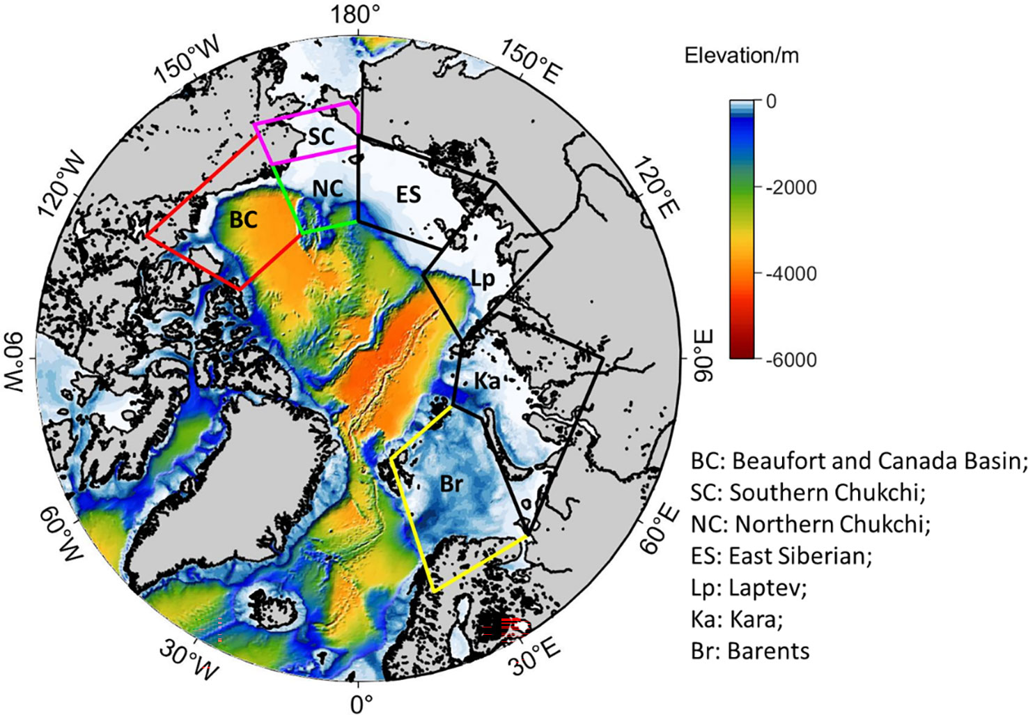
Figure 1 Map of the Arctic Ocean study area. The 7 boxes indicate the following regions: Beaufort and Canada Basin (BC); Northern Chukchi (NC); Southern Chukchi (SC); East Siberian (ES); Laptev (Lp); Kara (Ka); Barents (Br).

The model NPP is vertically integrated in the upper 110m and we use the sum of NPP from the three phytoplankton species. Monthly and seasonal sum of NPP (g C/m²/month) are calculated for each region. Nitrate (NO₃) has been proved to be a major limiting nutrient of NPP in many Arctic waters (Tremblay et al., 2008; Zhuang et al., 2020). Monthly and seasonal average of nitrate, sea-surface temperature (SST) and sea ice concentration (SIC) for each region are also extracted from model. Ice-free days ratio (IFR) is calculated with a criterion of SIC<10%, same as Crawford et al. (2020). Note that the NPP in Crawford et al. (2020) are only available in ice-free areas, and the model data include NPP in both ice-free and ice-covered areas.

2.2 JRA-55 Reanalysis data

JRA-55 reanalysis data has a ∼0.5625^° latitude/longitude spatial resolution and 3-hr temporal resolution. Near-surface winds are for the period June-September 1990-2014 are used to calculated (a) high-wind frequency (HWF) corresponding to the percentage of time when wind speed exceeds 10 m/s and (b) westerly wind frequency (WWF) corresponding to the percentage of time when zonal wind speed exceeds 0 m/s.

2.3 Multiple linear regression

2.3.1 Multiple linear regression NPP with IFR, SST, HWF, WWF

Based on satellite data, Crawford et al. (2020) applied the following multiple linear regression equation between NPP and physical environmental variables (IFR, SST, HWF, WWF) in the Arctic seas, here all variables were normalized for comparable scaling of variability:

$\begin{array}{ll}NPP=\alpha +{\beta }_{1}IFR+{\beta }_{2}SST+{\beta }_{3}HWF+{\beta }_{4}WWF& (1)\end{array}$

The aim of this study is to use the coupled ice-ocean-ecosystem model to further investigate mechanisms behind any significant correlations between NPP and physical environmental variables in different seas. We will first apply equation (1) with model results to validate the original model results, using seasonal and monthly model output for June to September of 1990-2014.

On the seasonal time scale, the model results (Table 1) show that NPP is significantly correlated with HWF in the Br (r=0.25, p<0.19) and SC (r=0.25, p<0.19), which agrees with the conclusions of Crawford et al. (2020) (Br: r=0.31, p<0.10; SC: r=0.32, p<0.10). Here, p<0.19 is chosen as the criterion for whether the correlation is significant for the model results, slightly different from p<0.10 in Crawford et al. (2020), as correlation displayed by the model results are slightly lower than the remote sensing data. In addition, the modeled NPP correlates with HWF in the NC (r=0.18, p<0.19), for which contains parts of shelf sea that similar to the SC. In the BC, the modeled NPP and HWF are not significantly correlated on a seasonal scale, consistent with Crawford et al. (2020), because strong stratification inhibits the replenishment of nutrients to surface layer by high winds (Nishino et al., 2020). There is a significant negative correlation between modeled NPP and WWF in the BC (r=-0.25, p<0.19), which is consistent with the results of Crawford et al. (2020) (r=-0.38, p<0.05).

TABLE 1

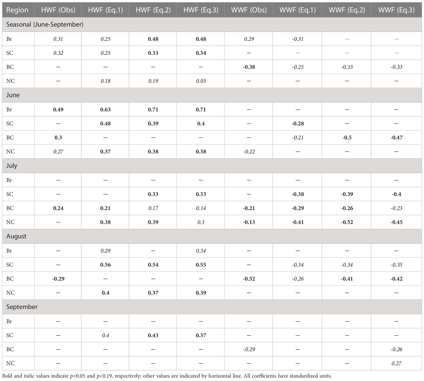
Table 1 Correlation coefficients between HWF/WWF and NPP of multiple linear regression models using Equation (1)-(3), and comparison with the observations (Crawford et al., 2020).

On the monthly time scales, modeled NPP is also highly correlated with HWF in several more months (Table 1) than that in Crawford et al. (2020). In particular, the model results show that NPP and HWF are significantly correlated in two months (June: r=0.63, p<0.05, August: r=0.29, p<0.19) in the Br, in three months (June: r=0.48, p< 0.05, August: r=0.56, p<0.05, September: r=0.40, p<0.19) in the SC, only in July (r=0.21, p<0.05) in the BC and in three months in the NC (June: r=0.37, p<0.05, July: r=0.38, p<0.05, August: r=0.40, p<0.05). While in Crawford et al. (2020), NPP and HWF are significantly correlated only in June (r=0.49, p<0.05) in the Br, none in the SC, in three months (June: r=0.30, p<0.05, July: r=0.24, p<0.05, August: r=-0.29, p<0.05) in the BC and only in June (r=0.27, p<0.10) in the NC.

Additionally, modeled NPP is significantly correlated with WWF for some months (Table 1), similar to Crawford et al. (2020). The modeled NPP and WWF are significantly correlated in three months (June: r=0.28, p<0.05, July: r=-0.38, p<0.05, August: r=-0.34, p<0.19) in the SC, none in the Br, in three months (June: r=-0.21, p<0.19, July: r=-0.29, p<0.05, August: r=-0.26, p<0.19) in the BC, and only in July (r=-0.41, p<0.05) in the NC. While in Crawford et al. (2020), NPP is non-significantly correlated with WWF in the Br and SC, but significantly correlated in three months (July: r=-0.21, p<0.05, August: r=-0.52, p<0.05, September: r=-0.29, p<0.10) in the BC and in two months (June: r= -0.22, p<0.10, July: r=-0.13, p<0.05) in the NC.

Overall, on the seasonal time scale, the model results show a significant correlation between NPP and HWF in the Br and SC, as well as a significant correlation between NPP and WWF in the BC, same conclusion from remote sensing results (Crawford et al., 2020). Modeled results also show significant correlation of NPP with HWF and WWF in several more individual months than remote sensing results. The validation of the model results with remote sensing results enable us to use the model to study the mechanisms of NPP response to wind variations. Taking advantage of more available variables (such as nutrients and other variables in depth under surface) than satellite data, we will also explore modifying variables in the regression equation (1).

2.3.2 Multiple linear regression of NPP with revised variables

Statistical analysis of the correlations between any two of the four variables in the right hand side of the equation (1) show that correlation is significant (p<0.05) between IFR and SST on both seasonal and monthly scales for all of the four seas (Table 2). HWF shows significant correlations with IFR and SST in August in the SC and in June in BC. WWF is significantly (p<0.05) correlated with IFR and SST in BC and NC for the season and most months because the thinning sea ice in these two seas become increasingly responsive to wind (Serreze and Meier, 2019). The presence of sea ice complicates the relationship between surface winds and SST, which may be further complicated with the strengthening of Beaufort High (Zhang and Zhang, 2018).

TABLE 2

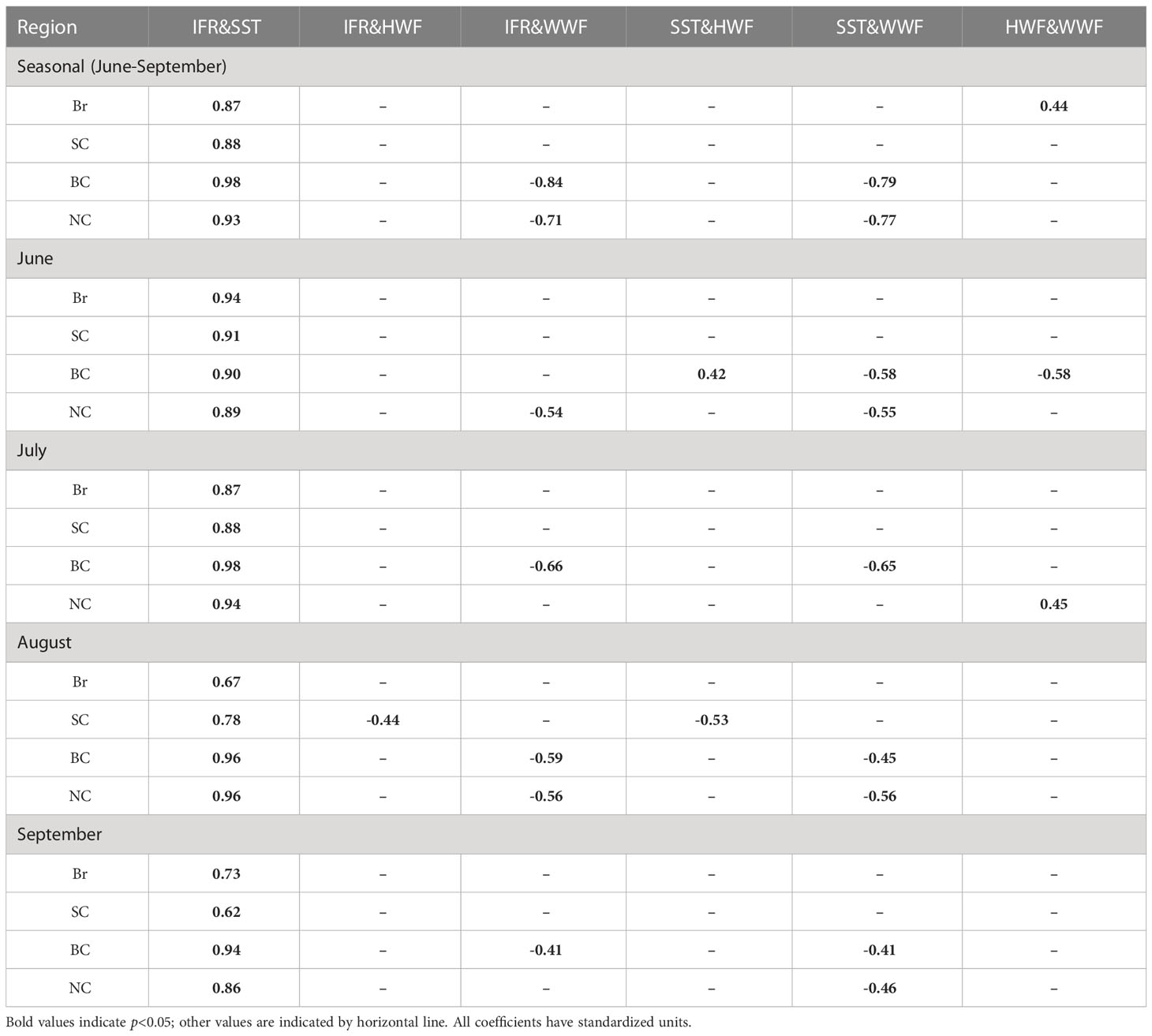
Table 2 Correlation coefficients between the four dependent variables in Equation (1) on both seasonal and monthly scales.

Since IFR and SST are the only pair that is statistically dependent on each other in all seas and on all time scales, and the quality of sea ice data is better than that of SST in remote sensing, we explore removes SST from equation (1) and yield:

$\begin{array}{ll}NPP=\alpha +{\beta }_{1}IFR+{\beta }_{2}HWF+{\beta }_{3}WWF& (2)\end{array}$

The results based on equation (2) show that the correlation between NPP and HWF/WWF is greatly improved both seasonally and monthly compared to the results of equation (1) (Table 1). Since the proposed mechanism behind NPP and wind involves changing nutrients in the euphotic zone (Crawford et al., 2020), and it’s beneficial to add NO₃ and yield:

$\begin{array}{ll}NPP=\alpha +{\beta }_{1}IFR+{\beta }_{2}N{O}_3+{\beta }_{3}HWF+{\beta }_{4}WWF& (3)\end{array}$

The regression results of equations (1)-(3) show similar type of significant correlations (Table 1), but with the addition of NO₃ in equation (3), the correlation coefficients and significance levels are improved over those using equations (1) and (2), suggesting that nutrients play an important role in linking NPP and wind events. Therefore, we will use equation (3) for the discussion in section 3.

3 Results and discussion

3.1 Correlations of NPP with HWF and WWF

On the seasonal time scale, the results (Table 1) based on equation (3) show further enhanced correlation (both coefficient and significance) between NPP and HWF mainly in the Br (r=0.48, p<0.05) and SC (r=0.34, p<0.05), versus remote sensing-based results (Br: r=0.31, p<0.10; SC: r=0.32, p<0.10). On monthly time scales, the correlations are also enhanced. NPP and HWF are significantly correlated in two months (June: r=0.71, p<0.05, August: r=0.34, p<0.19) in the Br; and in all four months (June: r=0.40, p<0.05, July: r=0.33, p<0.05, August: r=0.55, p<0.05 and September: r=0.37, p<0.05) in the SC. The correlation between NPP and HWF (r=0.03, p<0.19) passed significant level in the NC, but the correlation coefficient is almost zero, thus it is not considered as an effective significant correlation in this study. The model results can reflect the phenomenon of high winds enhanced NPP in the Br and SC, similar to the observed results (Crawford et al., 2020), and also enable us to include the NO₃ in the regression as one of the possible mechanisms. Our discussion on the correlation between NPP and HWF will therefore focus on the Br and SC.

Meanwhile, the correlation between NPP and WWF on the seasonal time scale is significant in the BC for both model (r=-0.33, p<0.19) and remote sensing (r=-0.38, p<0.05), but not significant in the NC for both model and remote sensing (Table 1). On monthly time scale, NPP and WWF are significantly correlated in all four months (June: r=-0.47, p<0.05, July: r=-0.23, p<0.19, August: r=-0.42, p<0.05 and September: r=-0.26, p<0.19) in the BC; in contrast, only in two months (July: r=-0.45, p<0.05, September: r=0.27, p<0.19) in the NC. Therefore, our discussion of the correlation between NPP and WWF will focus on the BC. The modeled correlation between NPP and WWF is similar as observations (Crawford et al., 2020) on seasonal scale, but stronger on monthly scales. This indicates that the model can capture NPP increase by the wind-driven upwelling mechanism in the BC, which will be analyzed in the latter section. The BC is strongly influenced by the Beaufort High, and the clockwise wind is the main driver of the upwelling along the shelf break. To facilitate the subsequent discussion, the WWF in equation (3) is changed to Easterly Wind Frequency (EWF), and the magnitude and significance of the NPP-EWF correlation remain the same as NPP-WWF, but the signs of correlation coefficients change from negative to positive. NPP in the Br, SC and BC are positively correlated with IFR and NO₃ seasonally and statistically significant for most months (p<0.05), indicating that increasing IFR and NO₃ in these three seas will lead to increasing NPP.

3.2 Monthly climatology of NPP, IFR, NO₃, HWF and EWF

It is necessary to analyze the modeled monthly average climatology of all variables in equation (3) and validate those based on remote sensing by Crawford et al. (2020). Spatially, the modeled NPP is strongest in the Arctic coastal seas, especially in the Br and SC (Figures 2A–D), similar to the remote sensing results. Temporally, the NPP of the four seas is relatively higher in June, July and August than in September (Figure 2E), and the stronger NPP in June than remote sensing results is because model results include NPP under sea ice cover, while remote sensing do not have data under ice-covered areas. Despite the differences, the magnitude, spatial and temporal distribution of NPP still reflect the general patterns seen from remote sensing results in Crawford et al. (2020).

FIGURE 2

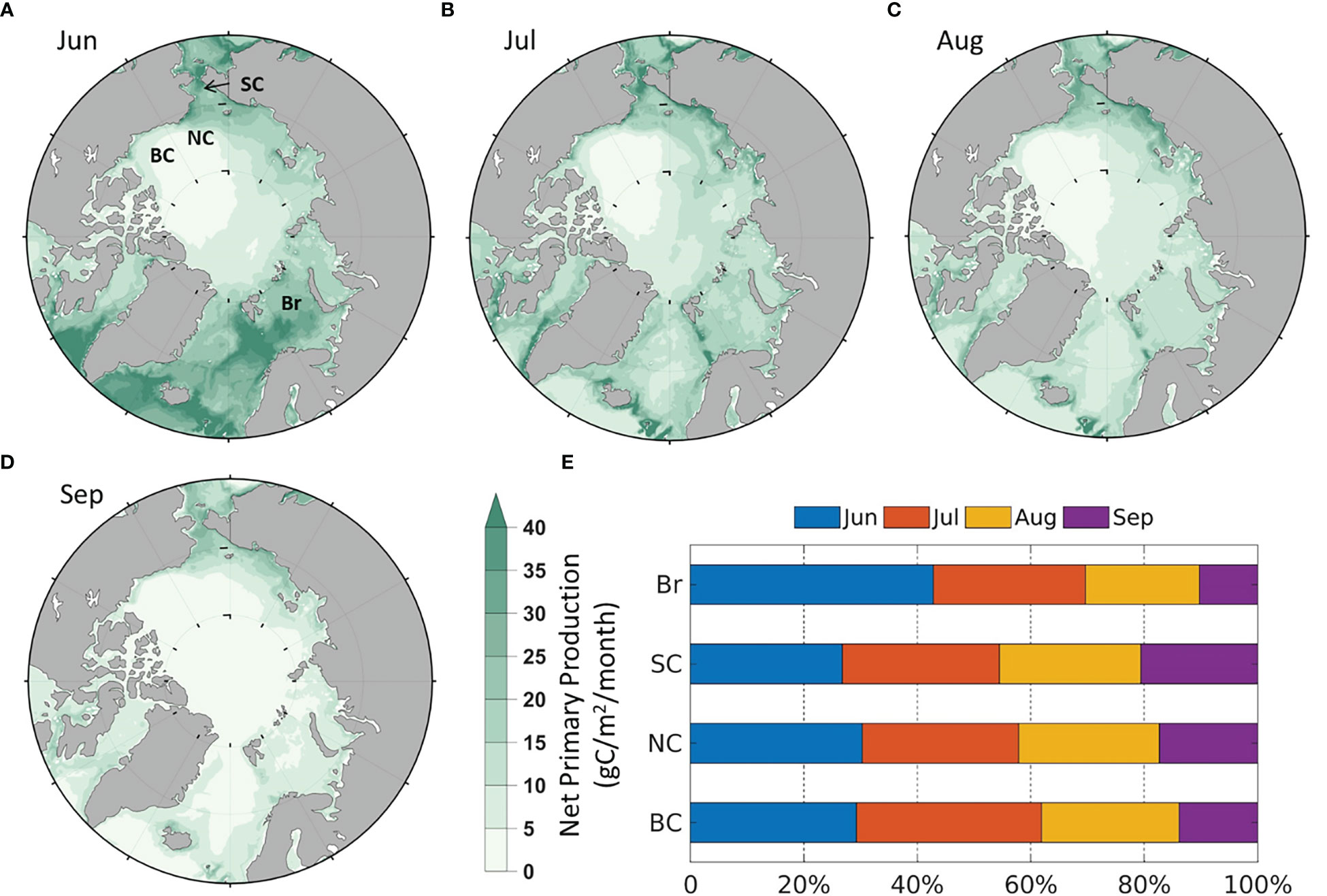
Figure 2 Modeled average monthly NPP (1990-2014) in (A) June; (B) July; (C) August; (D) September; (E) Average percentage of monthly contribution to the summer NPP by region.

IFR generally increases from June to September, but the time of ice retreat and the number of ice-free days are different by regions (Figure 3), which is partially responsible for regional monthly NPP differences in Figure 2. In June, the number of ice-free days is highest in the Br (Figure 3A), with over 25 ice-free days in the south Br. In July, ice-free days increase significantly in the SC, followed by the BC and NC (Figure 3B). In August and September, ice-free days in most of the Br and SC exceed 25 days, in contrast to less than 10 days in large part of the BC and NC (Figures 3C, D). Compared to the remote sensing (Crawford et al., 2020), the modeled monthly ice-free days and IFR distribution are very similar in the Br, but are slightly different in the other seas in some months. For example, in the SC in June (Figure 3A) as well as the BC and NC in July-September (Figures 3B–D), the modeled areas with more than 25 ice-free days are smaller and the differences of IFR between model and remote sensing results are ~5%-12% (Figure 3E).

FIGURE 3

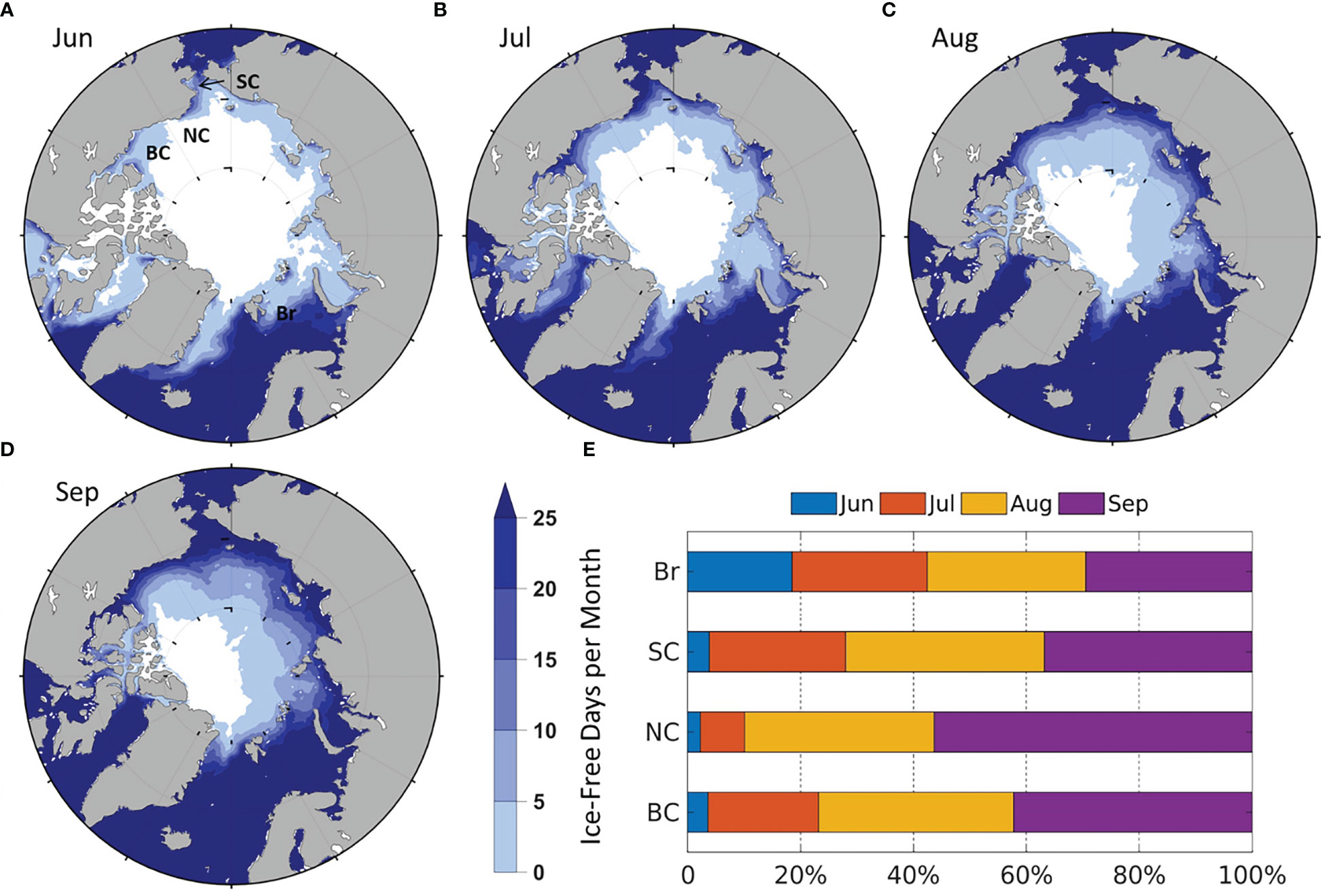
Figure 3 Modeled average number of ice-free days (1990-2014) in (A) June; (B) July; (C) August; (D) September. The average of zero days is colored white; (E) Average percentage of monthly contribution to summer IFR by region.

The modeled surface (0-20 m) averaged NO₃ is high in most of the Arctic shelf seas (over 5 mmol/m³) in June (Figure 4A) as they are still in pre-bloom stage except the south Br (<2 mmol/m³). NO₃ is relatively lower in the south Br in June (Figure 4A), because there are less sea ice cover to limit phytoplankton production (Figure 3A). Therefore, the input of nutrient-rich Pacific inflow water (Woodgate et al., 2012; Lin et al., 2019) are still evident in the SC in June, but the intrusion of nutrient-rich Atlantic water are less pronounced in the Br. NO₃ decrease in all four seas in July and August as nutrients are consumed by primary production (Figures 4B, C, E). In September, NO₃ starts to recover (Figures 4D, E), which may be associated with the deepening of the mixed layer due to sea surface cooling and higher HWF (Figure 5A). The magnitudes and spatial-temporal distributions of the modeled NO₃ are generally comparable to the gridded World Ocean Atlas 2018 (WOA2018, https://www.ncei.noaa.gov/archive/accession/NCEI-WOA18) in June-September. The modeled NO₃ in the BC in August and September (<0.5 mmol/m³) is close to the measurements (<1 mmol/m³) in August-September from 2008 to 2014 (Zhuang et al., 2018). The low NO₃ in the BC is due to the convergence of surface low nutrient water toward the center of the Beaufort Gyre (Carmack et al., 2008; Zhuang et al., 2018).

FIGURE 4

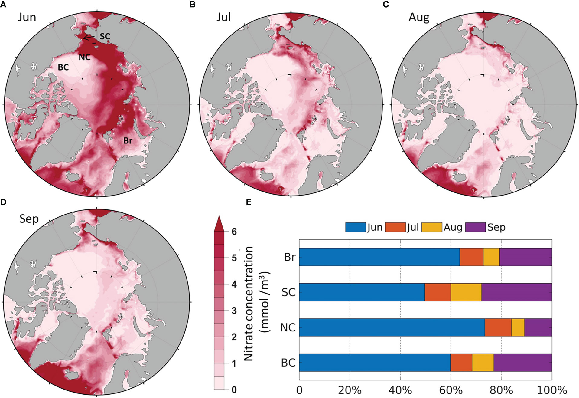
Figure 4 Modeled average monthly surface (0-20m) NO₃ (1990-2014) in (A) June; (B) July; (C) August; (D) September; (E) Average percentage of monthly contribution to summer NO₃ by region.

FIGURE 5

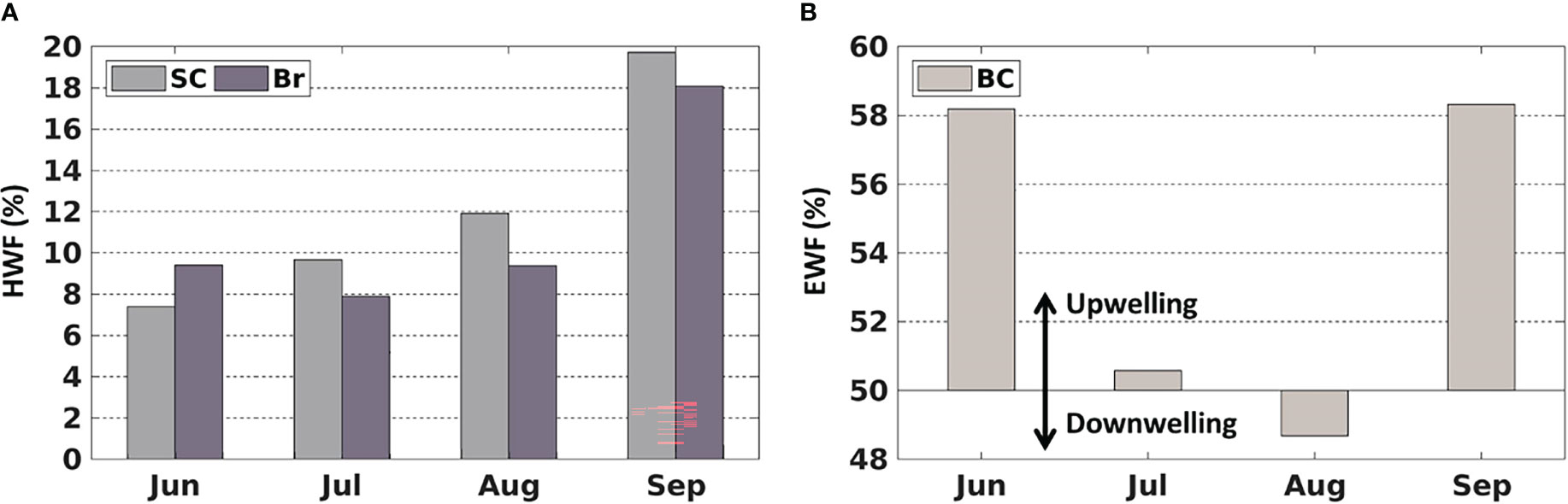
Figure 5 Average monthly (1990-2014) (A) high wind frequency (HWF) in the SC and Br and (B) easterly wind frequency (EWF) in the BC.

The HWF and EWF (Figure 5) are from the JRA-55 reanalysis data in this study. The temporal distribution of JRA-derived HWF is similar to that from ERA-I in Crawford et al. (2020), but magnitudes are generally higher in the SC and Br from June to September (Figure 5A), partly because JRA is in higher resolution (3 hourly, 0.25°) than ERA-I (6 hourly, 0.75°). JRA-derived HWF ranges of 7% -12% (SC) and 8%-10% (Br) in June-August, while ERA-derived HWF are 4% -7.5% (SC) and 5% -8% (Br). HWF in September is much higher at 20% (SC) and 18% (Br) (Figure 5A), which are higher than the ERA-derived HWF of 10% (SC) and 11% (Br). JRA-derived EWF is close to 50% in July and August with no dominant east-west wind, while larger (over 58%) in June and September, indicating that upwelling-favorable wind dominant in the BC. However, the magnitudes of JRA-derived EWF are notably smaller than those from ERA-I in June (58% vs. 66%) (Figure 5B).

3.3 Response of NO₃ and NPP to HWF in the Br and SC

The HWF influence on NPP is through its redistribution of NO₃, but increasing NPP also means increased consumption of NO₃, therefore the NO₃ response to HWF is both physical and biological. Consider the HWF influence and NPP activity are depth-sensitive, we divided the shallow Br and SC into the surface (0-20 m) and subsurface (20-50 m) layers for analysis. The seasonal (June to September) averaged NO₃ and vertically-integrated NPP in five highest (Br: 1991, 1994, 2006, 2009, 2010; SC: 1990, 1996, 2001, 2011, 2012) and five lowest (Br: 1990, 1993, 1998, 2000, 2011; SC: 1992, 1995, 2002, 2004, 2007) HWF years were calculated, as well as the statistical significance (using t-test) of the NO₃ and NPP relative differences of high minus low HWF years. Since sea ice retreat is widely considered to be the main cause of the increase in NPP in the Arctic Ocean, it is necessary to compare the relative magnitude of the impact of HWF and sea ice on NPP. Here the NPP relative differences (high minus low IFR years) were also calculated for the five highest (Br: 1992, 2006, 2007, 2012, 2013; SC: 1990, 1996, 2003, 2007, 2009) and five lowest (Br: 1993, 1997, 1998, 1999, 2003; SC: 1994, 1998, 2000, 2001, 2008) IFR years.

The HWF relative differences (Table 3) between high and low HWF years are 54.25% and 62.88% in the Br and SC, respectively, and are both statistically significant (p<0.05). The NPP relative increase due to high HWF (Table 3) is very similar in the Br (6.72%) and SC (6.53%). The magnitude of increase in surface NO₃ due to high HWF (Br: 0.18, SC: 0.15 mmol/m³) is smaller than the magnitude of decrease in the subsurface layer (Br: -0.78, SC: -0.88 mmol/m³) (Table 3). Assuming that all nutrients lost in the subsurface were mixed into the surface layer, then 0.60 (Br) and 0.73 mmol/m³ (SC) were consumed by primary production and other processes, which led to increases in NPP. For comparison, the IFR relative differences (Br: 35.67%, SC: 43.69%) are both statistically significant (p<0.05) and similar to those for HWF. The NPP relative increase caused by high IFR (Table 3) is much greater in the SC (17.46%) than in the Br (9.98%), and both are greater than the NPP relative increase caused by high HWF in these two seas, respectively. This indicates that in the Br and SC, particularly the SC, IFR is currently still the dominant process leading to an increase in NPP. However, with further reduction in Arctic sea ice in the future, the relative influence of IFR will decrease, while the relative influence of HWF will continue to become greater.

TABLE 3

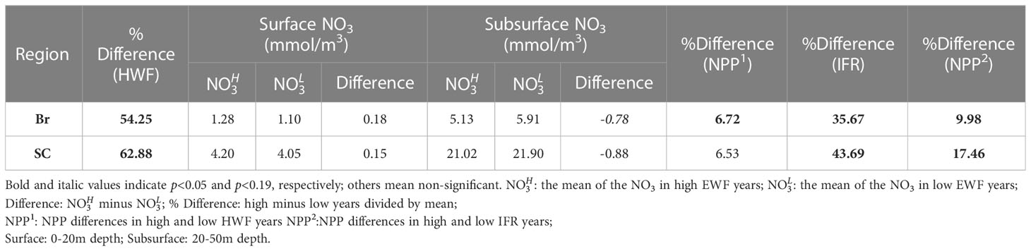
Table 3 Changes to seasonal HWF (%), NO₃ (mmol/m³), NPP (g C/m²/month) and IFR (%) in high and low years in the Br and SC.

Since the increased highly nutrient Atlantic inflow into the Br from 1993 to 2016 (Oziel et al., 2020) and the increased highly nutrient Pacific inflow into the SC from 1990 to 2015 (Woodgate, 2017), there will be an increasing trend in nutrients in both seas. To evaluate how much the effect of HWF on NO₃ is influenced by these long-term trends, we recalculated the differences using detrended data. The results show only a small change in NO₃ differences after detrending compared to differences before detrending, with no change in statistical significance, indicating that the long-term trends have less influence on the results of our analysis.

The statistical analysis above shows that high HWF leads to high surface and low subsurface NO₃ as well as high vertical-integrated NPP. The results of equation (3) indicate that NPP in the SC is significantly correlated with HWF. However, in high and low HWF years, the HWF relative difference is statistically significant, while the NPP relative difference is statistically insignificant. We choose a zonal average section of the SC as an example to analyze the spatial variation of NO₃ and NPP responses to high and low HWF (Figures 6, 7). In all years, the seasonally averaged distribution of HWF increased gradually from south to north (Figure 8A), while the seasonal NPP (Figure 8B) and NO₃ (Figures 6A, B) decrease gradually, but the differences in HWF, NPP and NO₃ between high and low HWF years are not remarkable in the south and higher in the north (Figures 8, 6C). In high HWF years, the locations of the increases in surface NO₃ (Figure 6C) and NPP (Figure 7C) in the north coincide, suggesting that the higher HWF in the north led to increases in surface NO₃ and NPP.

FIGURE 6

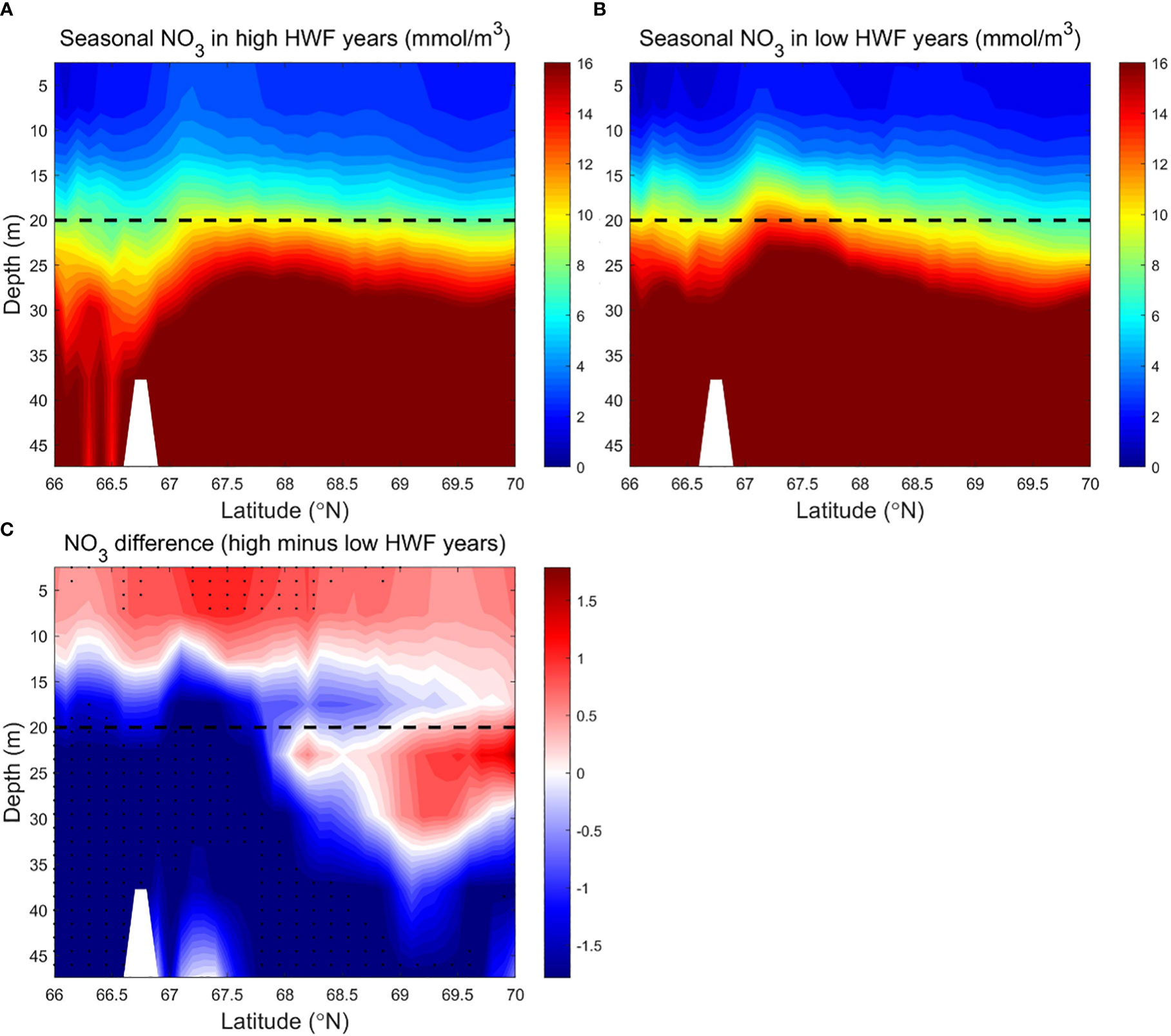
Figure 6 Modeled seasonally (June to September) averaged NO₃ (mmol/m³) in the SC in the (A) high (1990, 1996, 2001, 2011, 2012) and (B) low (1992, 1995, 2002, 2004, 2007) HWF yeas, and (C) their differences (high minus low). The dashed lines denote 20 m depth. In Figure 6C, black dots denote where p<0.19, because there is no area where p<0.05.

FIGURE 7

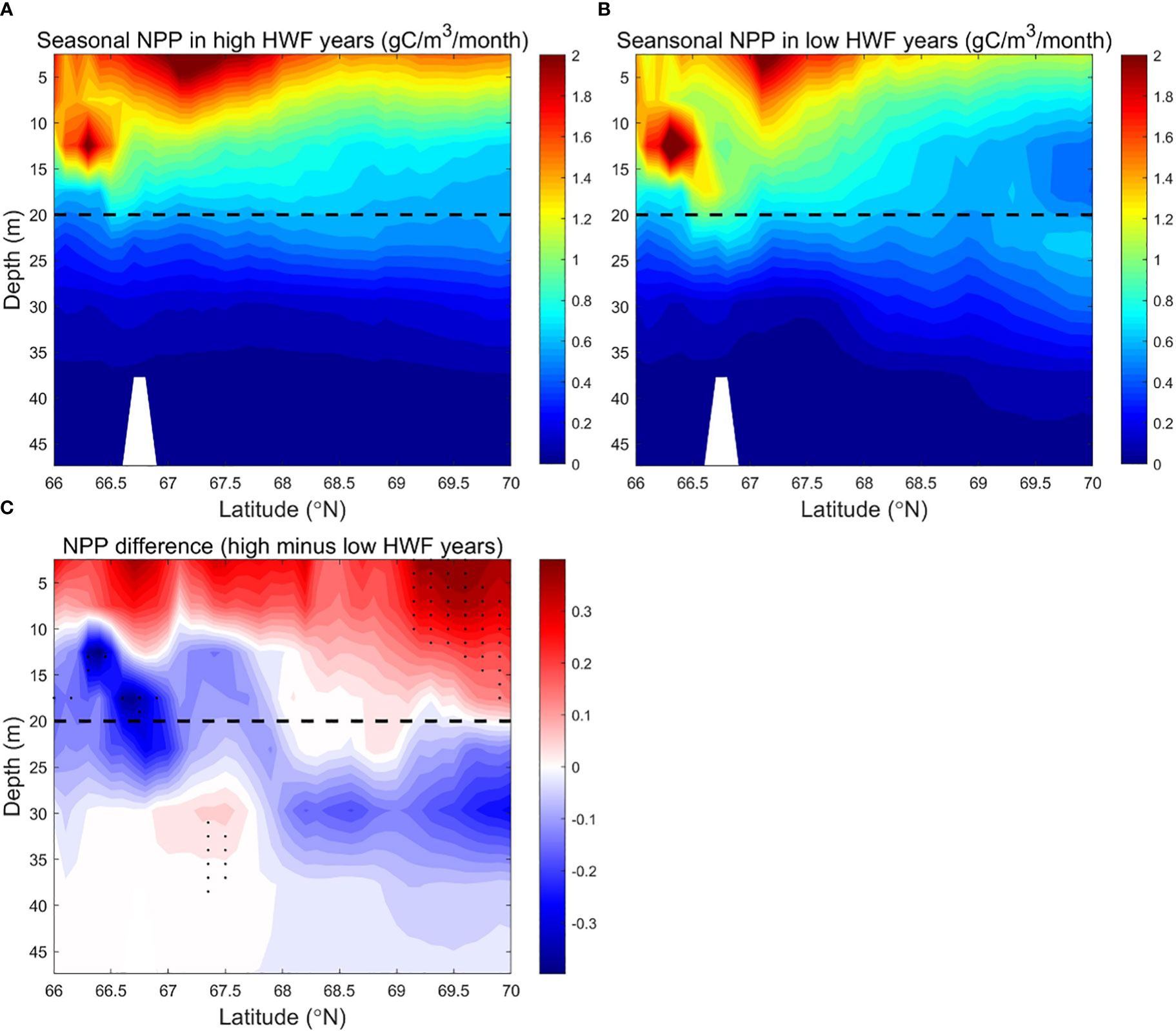
Figure 7 Modeled seasonally (June to September) averaged NPP (g C/m3/month) in the SC in the (A) high (1990, 1996, 2001, 2011, 2012) and (B) low (1992, 1995, 2002, 2004, 2007) HWF yeas, and (C) their differences (high minus low). The dashed lines denote 20 m depth. In Figure 7C, black dots denote where p<0.05.

FIGURE 8

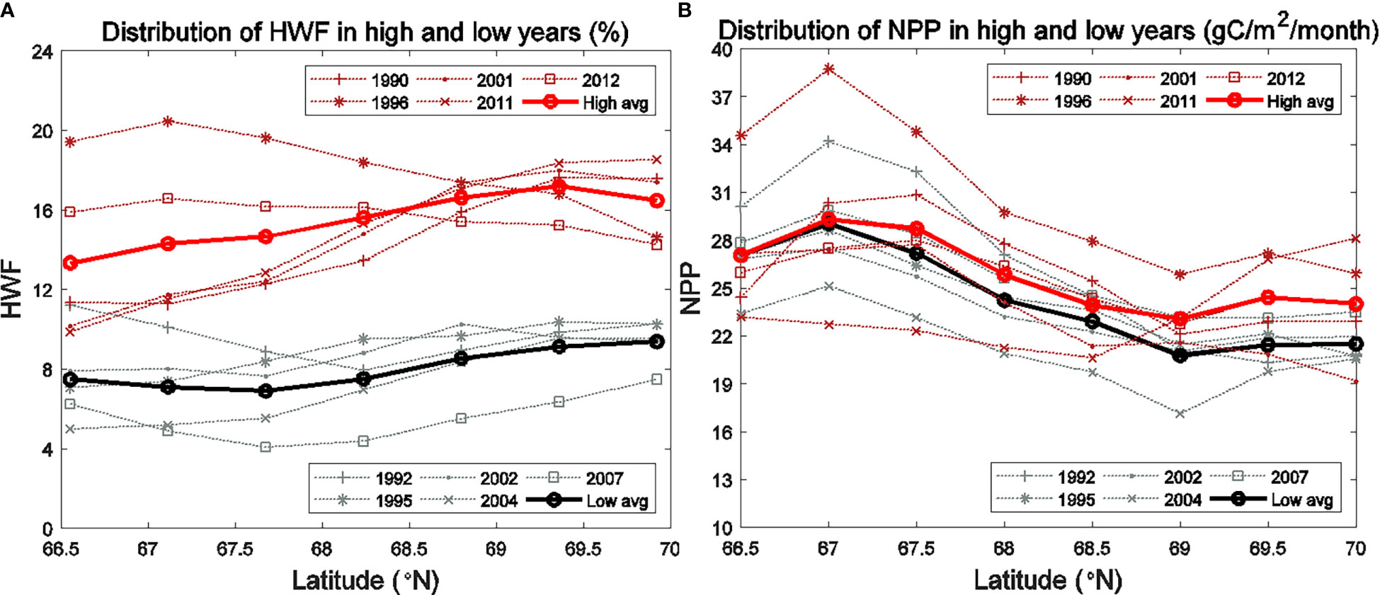
Figure 8 Seasonally (June to September) averaged (A) HWF and (B) modeled vertically-integrated NPP for the high (1990, 1996, 2001, 2011, 2012) and low (1992, 1995, 2002, 2004, 2007) HWF years in the SC.

Subsurface NO₃ (>16 mmol/m³) in all years is much higher than the surface layer (<8 mmol/m³) in most areas (Figures 6A, B). The vertical distribution and magnitudes of modeled NO₃ in SC are consistent with observations, such as Figures 3-5 in Lee et al. (2007) and Figures 4-5C and 6-10C in Lowry et al. (2015). In August, section across the Chukchi Sea along 170°W is generally characterized with high-temperature, low-salinity, nutrient-poor Alaskan Coastal Water (ACW) in surface layer and low-temperature, high-salinity, nutrient-rich Chukchi Summer Water (CSW) in the subsurface layer (Qi et al., 2022). The strong vertical stratification in summer causes a rapid attenuation of turbulent mixing (Randelhoff et al., 2017), which maintains the strong vertical gradient of NO₃, along with other factors, such as the high-nutrient pacific inflow, the supplementation of organic matter decomposition on the adjacent shelf (Tremblay et al., 2015) and biological consumption (Zhuang et al., 2021).The strong vertical gradient of NO₃ remains even in high HWF years (Figure 6A). The distribution of NPP in the south region is higher than that in the north region, and the surface layer is much higher than the subsurface layer (Figures 7A, B). The higher NPP in the south region is due to higher nutrients and more ice-free days (Figures 3A-D), that increase light availability (Song et al., 2021) and growth time of phytoplankton (Arrigo and Van Dijken, 2011). Lower subsurface NPP is due to lower light that limits phytoplankton growth (Tremblay and Gagnon, 2009).

Large vertical differences in NO₃ in the SC make high winds more efficient in raising surface NO₃, which results in a significant increase in NPP from high HWF. Higher HWF increases NO₃ and NPP in the upper 0-10m in the south and 0-20m in the north, but reduces NO₃ and NPP in the subsurface layer (Figures 6C, 7C). The decrease in subsurface NO₃ decrease is 1.2-1.7 mmol/m³ (relative change of -7.5% to -10.6%), which is larger than the increase in surface NO₃ of 0.5-1.0 mmol/m³ (relative change of 3.1% to 6.2%) (Figure 6C).The decrease in subsurface NPP of about 0.1-0.3 g C/m³/month (relative change of -5% to -15%) is smaller than the increase in surface NPP of about 0.2-0.4 g C/m³/month (relative change of 10% to 20%) (Figure 7C). The relatively large increase in surface NPP reduces the relative increase in surface NO₃. The differences of NO₃ and NPP are statistically significant only in sparse areas (Figures 6C, 7C) in both surface and subsurface layers, probably because the NO₃ brought up by higher HWF and the corresponding variation in NPP are quickly altered by other factors in most areas.

Although the NPP differences between high and low HWF years are not statistically significant, the sections of NO₃ and NPP still reflect the mechanism by which HWF affects NPP through redistribution of NO₃.The mechanism of NPP response to higher HWF through vertical mixing of NO₃ from nutrient-rich subsurface to nutrient-poor surface layer, causing an increase in surface NO₃ and a decrease in subsurface NO₃. However, the amount of nutrient modification by other physical processes and biological growth can alter the extent and degree of high wind impacts, limiting statistically significant changes in surface and subsurface NO₃ and NPP in high HWF years only in small patches.

3.4 Response of NO₃ and NPP to EWF in the BC

We used the seasonal (June-September) averaged NO₃ and NPP for the five highest (1998, 2007, 2008, 2010, 2011) and five lowest (1991, 1992, 1994, 1996, 2002) EWF years to analyze the redistribution of NO₃ by the EWF and the effect on NPP. To compare the relative effects of sea ice and EWF on NPP, we also calculated the NPP relative differences (high minus low) for the five highest (1998, 2008, 2010, 2011, 2012) and five lowest (1991, 1992, 1994, 1996, 2002) IFR years

The EWF relative difference (high minus low) between high and low EWF years is 51.52% and statistically significant (p<0.05) (Table 4). The NPP relative increase due to high EWF in the BC (67.64%) (Table 4) is much greater than that due to high HWF in the Br and SC (Table 3). This is because the BC is much deeper than either of these seas (Figure 1) and the upwelling caused by high EWF can carry deeper and higher NO₃ to the surface (0.09 mmol/m³) and subsurface (0.10 mmol/m³) (Table 4). The magnitude of the NO₃ increase is smaller than in the Br and SC, since the increase in NO₃ is mainly at the shelf break where upwelling is strongest and is relatively low in the north Canada Basin. As a comparison, the IFR relative difference (158.37%) is statistically significant (p<0.05) and is almost three times the difference in EWF. However, the NPP relative increase caused by high IFR (64.76%) (Table 4) is close to that caused by high EWF (67.64%), suggesting that the increase in NPP due to EWF in the BC is comparable to the increase caused by IFR.

TABLE 4

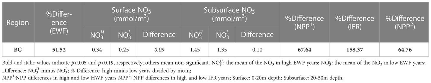
Table 4 Changes to seasonal EWF (%), NO₃ (mmol/m³), NPP (g C/m²/month) and IFR (%) in high and low years in the BC.

The relative differences in EWF and NPP for both high and low EWF years are statistically significant, consistent with the statistical correlation between NPP and EWF in the BC from equation (3). We calculated the zonal average of seasonal NO₃ and NPP and their differences (high minus low) for the five highest and five lowest EWF years, in order to further analyze the spatial variability of the NO₃ and NPP responses to high and low EWF (Figures 10, 11). Both seasonal EWF and NPP show a gradual southward increase from the Canada Basin to the Beaufort Sea shelf break in all years, but the NPP near the shelf break in high EWF years is almost twice as high as in low EWF years (Figure 9). The higher NPP in the south is so co-regulated multiple factors: (1) more ice-free days (Figures 3A–D), (2) more light, (3) more nutrients in all years (Figures 10A, B) and (4) more additional nutrients brought up by upwelling in high EWF years (Figure 10C). The EWF difference (high minus low) is smaller in the south (near the shelf-break) than in the north, suggesting that high EWF at the shelf break is a key factor in causing the increase in NPP. In the Canada Basin, while the EWF difference increases from south to north, the NPP difference decreases exponentially.

FIGURE 9

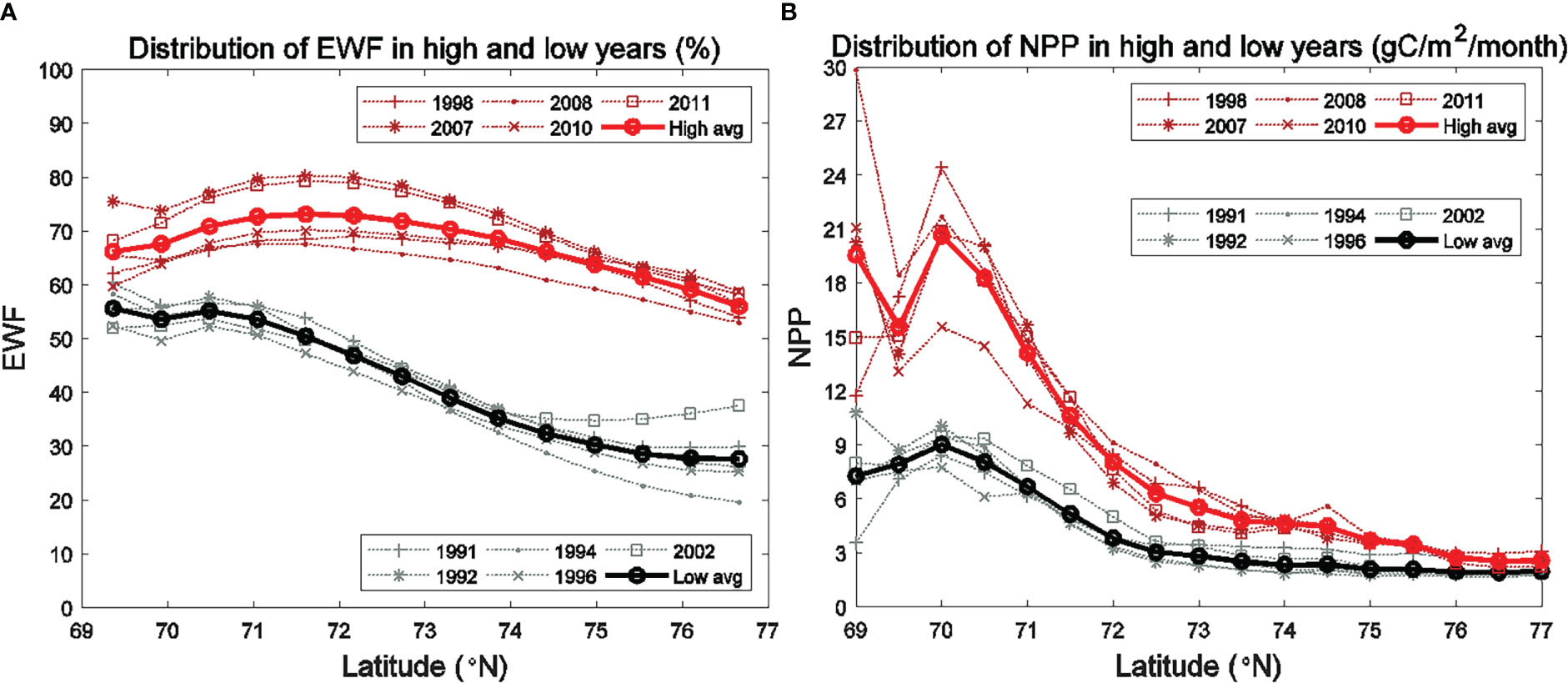
Figure 9 Seasonally (June to September) averaged (A) EWF and (B) modeled vertically-integrated NPP for the high (1998, 2007, 2008, 2010, 2011) and low (1991, 1992, 1994, 1996, 2002) EWF years in the BC.

FIGURE 10

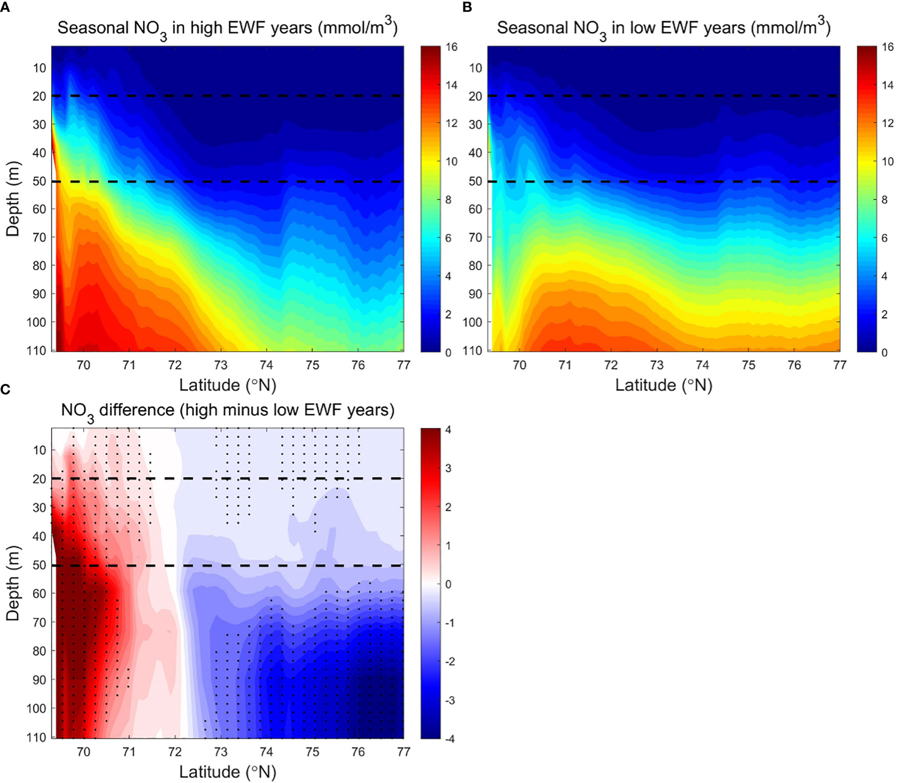
Figure 10 Modeled seasonally (June to September) averaged NO₃ (mmol/m³) in the BC in (A) high (1998, 2007, 2008, 2010, 2011) and (B) low (1991, 1992, 1994, 1996, 2002) EWF yeas, and (C) their differences (high minus low). The dashed lines denote 20 m and 50 m depth separately. In Figure 10C, black dots denote where p<0.05.

FIGURE 11

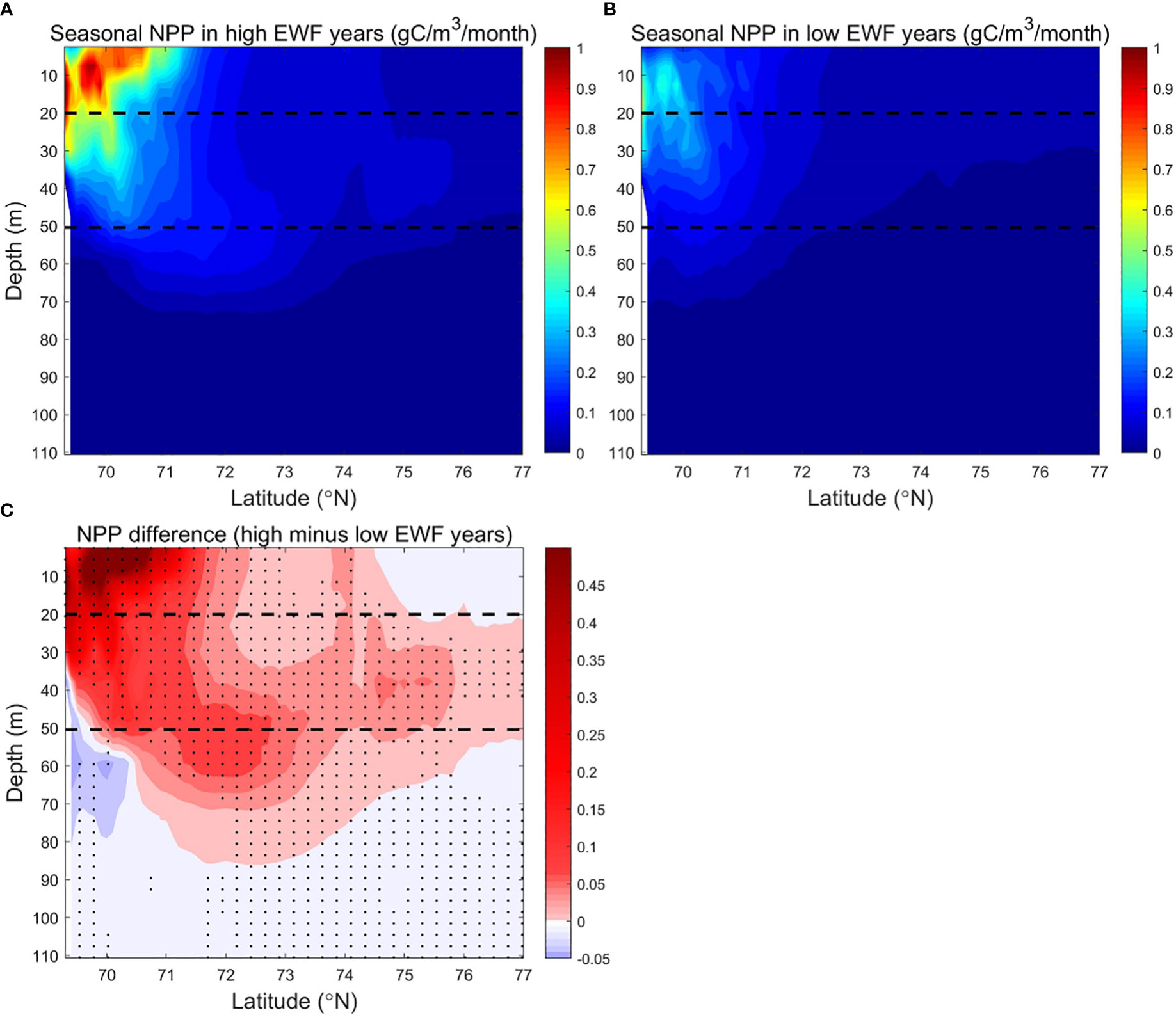
Figure 11 Modeled seasonally (June to September) averaged NPP (g C/m3/month) in the BC in (A) high (1998, 2007, 2008, 2010, 2011) and (B) low (1991, 1992, 1994, 1996, 2002) EWF yeas, and (C) their differences (high minus low). The dashed lines denote 20 m and 50 m depth separately. In Figure 11C, black dots denote where p<0.05.

The strong vertical stratification caused by the accumulation of freshwater (Proshutinsky et al., 2009) prevents the upward transport of high NO₃ from subsurface Pacific summer waters (Tremblay et al., 2008; Timmermans and Toole, 2022). Modeled NO₃ is low (<2 mmol/m³) in most areas of the surface and subsurface layers, and higher (>8 mmol/m³) below the subsurface layer to 110 m. NO₃ in the south (<73.5°N) is higher (<12-16 mmol/m³) than in the north (<8-10 mmol/m³) (Figures 10A, B). The deeper vertical distribution of high NO₃ reduces the efficiency of high HWF in raising surface NO₃, resulting in a non-significant correlation between NPP and HWF in the BC.

The high EWF supports more upwelling effects at the shelf break to below 110 m depth (Figures 10A, C). Surface NO₃ differences near the shelf break are 1-2 mmol/m³ (relative change of 6.25% to 12.5%), less than the 2-4 mmol/m³ (relative change of 12.5% to 25%) of subsurface (Figure 10C). The smaller surface NO₃ differences are due to higher biological depletion, and thus the corresponding surface NPP differences are 0.10-0.45 g C/m³/month (relative change of 10% to 45%), larger than 0.05-0.20 g C/m³/month (relative change of 5% to 20%) of subsurface (Figure 11C). From the shelf break to the Canada Basin center, as the high NO₃ transported northwards by Ekman decreases with distance, the surface and subsurface NO₃ differences decrease exponentially to near zero in the center of the Basin (Figure 10C). The NPP differences corresponds to the NO₃ difference, which also decreases northwards in the surface and subsurface layers, with the surface NPP difference approaching zero by the center of the Basin and remaining positive in the subsurface layer (Figure 11C). In high EWF years, the surface NPP decreases faster than the subsurface, resulting in a greater south-north gradient than the subsurface (Figure 11A). High EWF tends to correspond to stronger Beaufort gyre strength and stronger down-welling in the Canada Basin center (Proshutinsky et al., 2009; Yang, 2009), with subsidence of higher production and nutrient-poor surface water leading to positive NPP differences in the subsurface and negative NO₃ differences in the deeper (>50 m) layers. NO₃ differences show a pathway of nutrients movement along the upwelling of the shelf break, northward Ekman transport in the surface layer and subsidence in the north basin region (Figure 10C). On this pathway, NPP differences are clearly causally related to NO₃ differences. NO₃ differences in the surface and subsurface layers are positive in most areas, except in the Canada Basin center where the NO₃ differences are close to zero, and the NPP differences in these areas are positive and statistically significant (Figure 11C).

The NPP difference is statistically significant in high and low EWF years. The cross-section of EWF, NO₃ and NPP reveal that the mechanism for the response of NPP to higher EWF is the uplift of lower high nutrients at the shelf break, northward Ekman transport in the surface layer and subsidence in the north basin region. Although the EWF differences are lower at the shelf break than in the north Canada Basin, the effects of EWF on NO₃ and NPP are strongest at the shelf break.

4 Conclusions

More open areas and growing seasons have led to increased primary production across the Arctic Ocean (Lewis et al., 2020), however, with fewer attentions paid to high wind events which could also trigger enhanced NPP (Crawford et al., 2020). The occurrence of storm is increasing in the Arctic Ocean (locally generated or imported from mid-low latitudes), especially in summer and autumn. Both high wind and upwelling-favorable wind can significantly increase NPP in some Arctic seas from remote sensing data (Crawford et al., 2020). Here we used the RASM model to further study the mechanisms by which wind affects nutrients distribution and primary production in different Arctic seas. The multiple linear regression analysis of model results (Table 1) and modeled monthly climatology of NPP, IFR and NO₃ are comparable to remote sensing and other observations, and therefore adequate for studying the underlying mechanisms and the spatial and temporal distribution of nutrients and NPP variations under different wind conditions.

Nutrients variations play important roles in the NPP response to HWF/EWF. Firstly, high nutrient differences between the shallow surface and subsurface layers below 50 m in the Br and SC allow significant effects of high wind mixing on surface nutrients and primary production enhancement. According to five high and five low HWF years along a zonally averaged section of HWF, NO₃, and NPP in the SC, we found that high HWF promotes the NO₃ relative increase in the surface is less than the decrease in the subsurface, suggesting that part of the surface NO₃ have been consumed by biological production and lead to larger relative increase of NPP in the surface. Higher HWF in the north mixes deeper NO₃ to the surface layer, and thus leads to more NPP increase, while the response processes are nonlinear and may be altered by other physical and biological processes in most areas. Secondly, higher nutrients in the BC are at greater depths with smaller nutrients difference in the upper 50m, and thus high winds are not as efficient at increasing surface nutrients and primary production in this area as they are in the Br and SC, so the response of NPP to HWF is significant in the Br and SC, but not in the BC. South-north sections show that high-EWF upwelling effects on NO₃ and NPP increases are strongest at the Beaufort Sea shelf break. High EWF further enhances south-north differences in NO₃ and NPP by promoting upwelling at the south and downwelling at the north. The mechanism of the NPP response to high EWF is through enhanced upwelling near the shelf break, carrying high NO₃ from depth (>100 m) to the upper layer, northward Ekman transport of higher nutrients in the upper layers, and sinking of surface higher production and nutrient-poor water in the Canada Basin center. As sea ice retreats, seasonal NPP increases not only with IFR but also with increasing HWF/EWF. The IFR remains one of the dominant factors for the summer NPP increase in the Br and SC, as the relative NPP increase caused by HWF (Br: 6.73%, SC: 6.53%) is smaller than that caused by IFR (Br: 9.98%, SC: 17.46%) (Table 3). In contrast, relative NPP increase caused by EWF (67.56%) is very close to that by IFR (64.76%, Table 4), indicating that the impact by high EWF on summer NPP is comparable to that by sea ice reduction in the BC.

Changes in wind strength and regimes can also significantly influence biogeochemical cycles, especially in highly productive coastal seas and shelf break regions. It is critical to improve our understanding on the mechanisms of those variability in biological production that can affect the carbon sink and marine ecosystems. High-resolution climate models are proved to be capable of capturing the statistical relationships between the NPP and different wind regimes in the Arctic seas. The analysis based on model results provides more temporal and spatial details and improved understanding on the mechanism of the NO₃ and NPP response to short-term high wind and upwelling-favorable wind events. With further reductions in Arctic sea ice, the effect of IFR gradually shifts northwards and the effect of winds on NPP becomes progressively more prominent. Keeping up to date with the corresponding changes in the carbon cycle and marine ecosystems in different Arctic seas for future winds variation is necessary.

Data availability statement

The original contributions presented in the study are included in the article/supplementary material. Further inquiries can be directed to the corresponding author.

Author contributions

MJ designed this study. AX performed analysis and wrote the manuscript and prepared the tables and figures. DQ and YW revised the manuscript. All authors edited the manuscript. All authors contributed to the article and approved the submitted version.

Funding

This work was supported by the National Key Research and Development Program of China (2019YFE0114800), the National Natural Science Foundation of China (42176230, 41941013); the Ocean Negative Carbon Emissions (ONCE) Program, Key Deployment Project of Centre for Ocean Mega-Research of Science; Natural Science Foundation of Fujian Province, China (2019J05148); Chinese Academy of Sciences (CAS) (grant no. COMS2020Q12).

Acknowledgments

We would like to acknowledge helpful discussions with Jihai Dong during the development of this manuscript.

Conflict of interest

The authors declare that the research was conducted in the absence of any commercial or financial relationships that could be construed as a potential conflict of interest.

Publisher’s note

All claims expressed in this article are solely those of the authors and do not necessarily represent those of their affiliated organizations, or those of the publisher, the editors and the reviewers. Any product that may be evaluated in this article, or claim that may be made by its manufacturer, is not guaranteed or endorsed by the publisher.

References

Aksenov Y., Popova E., Yool A., Nurser G. (2015). Predicting the Arctic ocean environment in the 21st century. EGU Gen. Assembly Conf. Abstracts, 13950.

Google Scholar

Ardyna M., Babin M., Gosselin M., Devred E., Rainville L., Tremblay J.-É. (2014). Recent Arctic ocean sea ice loss triggers novel fall phytoplankton blooms. Geophysical Res. Lett. 41 (17), 6207–6212. doi: 10.1002/2014gl061047

CrossRef Full Text | Google Scholar

Arrigo K. R., Van Dijken G. L. (2011). Secular trends in Arctic ocean net primary production. J. Geophysical Res. 116 (C9), 09011. doi: 10.1029/2011jc007151

CrossRef Full Text | Google Scholar

Arrigo K. R., Van Dijken G. L. (2015). Continued increases in Arctic ocean primary production. Prog. Oceanography 136, 60–70. doi: 10.1016/j.pocean.2015.05.002

CrossRef Full Text | Google Scholar

Arrigo K. R., van Dijken G., Pabi S. (2008). Impact of a shrinking Arctic ice cover on marine primary production. Geophysical Res. Lett. 35 (19), 1–6. doi: 10.1029/2008gl035028

CrossRef Full Text | Google Scholar

Årthun M., Eldevik T., Smedsrud L. H., Skagseth Ø., Ingvaldsen R. B. (2012). Quantifying the influence of Atlantic heat on barents Sea ice variability and retreat*. J. Climate 25 (13), 4736–4743. doi: 10.1175/jcli-d-11-00466.1

CrossRef Full Text | Google Scholar

Bates N. R., Moran S. B., Hansell D. A., Mathis J. T. (2006). Arctic Ocean due to sea-ice loss. Geophysical Res. Lett. 33 (23), 23609. doi: 10.1029/2006gl027028

CrossRef Full Text | Google Scholar

Cai W. J., Chen L., Chen B., Gao Z., Lee S. H., Chen J., et al. (2010). Decrease in the CO₂ uptake capacity in an ice-free Arctic ocean basin. Science 329 (5991), 556–559. doi: 10.1126/science.1189338

PubMed Abstract | CrossRef Full Text | Google Scholar

Carmack E., Barber D., Christensen J., Macdonald R., Rudels B., Sakshaug E. (2006). Climate variability and physical forcing of the food webs and the carbon budget on panarctic shelves. Prog. Oceanography 71 (2-4), 145–181. doi: 10.1016/j.pocean.2006.10.005

CrossRef Full Text | Google Scholar

Carmack E., Chapman D. C. (2003). Wind-driven shelf/basin exchange on an Arctic shelf: The joint roles of ice cover extent and shelf-break bathymetry. Geophysical Res. Lett. 30 (14), 1778. doi: 10.1029/2003gl017526

CrossRef Full Text | Google Scholar

Carmack E., McLaughlin F. A., Yamamoto-Kawai M., Itoh M., Shimada K., Krishfield R., et al. (2008). Freshwater storage in the northern ocean and the special role of the Beaufort gyre. Arctic–Subarctic Ocean Fluxes 145–169. doi: 10.1007/978-1-4020-6774-7_8

CrossRef Full Text | Google Scholar

Castro de la Guardia L., Garcia-Quintana Y., Claret M., Hu X., Galbraith E. D., Myers P. G. (2019). Assessing the role of high-frequency winds and Sea ice loss on Arctic phytoplankton blooms in an ice-Ocean-Biogeochemical model. J. Geophysical Res.: Biogeosci 124 (9), 2728–2750. doi: 10.1029/2018jg004869

CrossRef Full Text | Google Scholar

Crawford A. D., Krumhardt K. M., Lovenduski N. S., Dijken G. L., Arrigo K. R. (2020). Summer high-wind events and phytoplankton productivity in the Arctic ocean. J. Geophysical Res.: Oceans 125 (9), 1–17. doi: 10.1029/2020jc016565

CrossRef Full Text | Google Scholar

Farmer J. R., Sigman D. M., Granger J., Underwood O. M., Fripiat F., Cronin T. M., et al. (2021). Arctic Ocean stratification set by sea level and freshwater inputs since the last ice age. Nat. Geosci. 14 (9), 684–689. doi: 10.1038/s41561-021-00789-y

CrossRef Full Text | Google Scholar

Gao Y., Zhang Y., Chai F., Granskog M. A., Duarte P., Assmy P. (2022). An improved radiative forcing scheme for better representation of Arctic under-ice blooms. Ocean Model. 177, 102075. doi: 10.1016/j.ocemod.2022.102075

CrossRef Full Text | Google Scholar

Harada Y., Kamahori H., Kobayashi C. (2016). The JRA-55 reanalysis representation of atmospheric. J. Meteorological Soc. Japan. Ser. II. 94 (3), 269–302 doi: 10.2151/jmsj

CrossRef Full Text | Google Scholar

Ingvaldsen R. B., Assmann K. M., Primicerio R., Fossheim M., Polyakov I. V., Dolgov A. V. (2021). Physical manifestations and ecological implications of Arctic atlantification. Nat. Rev. Earth Environ. 2 (12), 874–889. doi: 10.1038/s43017-021-00228-x

CrossRef Full Text | Google Scholar

Jin M., Deal C., Maslowski W., Matrai P., Roberts A., Osinski R., et al. (2018). Effects of model resolution and ocean mixing on forced ice-ocean physical and biogeochemical simulations using global and regional system models. J. Geophysical Res.: Oceans 123 (1), 358–377. doi: 10.1002/2017jc013365

CrossRef Full Text | Google Scholar

Jin M., Popova E. E., Zhang J., Ji R., Pendleton D., Varpe Ø., et al. (2016). Ecosystem model intercomparison of under-ice and total primary production in the Arctic ocean. J. Geophysical Res.: Oceans 121 (1), 934–948. doi: 10.1016/j.csr.2007.05.009

CrossRef Full Text | Google Scholar

Kerkar A. U., Tripathy S. C., Hughes D. J., Sabu P., Pandi S. R., Sarkar A., et al. (2021). Characterization of phytoplankton productivity and bio-optical variability in a polar marine ecosystem. Prog. Oceanography 195, 102573. doi: 10.1016/j.pocean.2021.102573

CrossRef Full Text | Google Scholar

Lee S. H., Whitledge T. E., Kang S. H. (2007). Recent carbon and nitrogen uptake rates of phytoplankton in Bering strait and the chukchi Sea. Continental shelf Res. 27 (17), 2231–2249. doi: 10.1016/j.csr.2007.05.009

CrossRef Full Text | Google Scholar

Lewis K. M., Van Dijken G., Arrigo K. R. (2020). Changes in phytoplankton concentration now drive increased Arctic ocean primary production. Science 369 (6500),198–202. doi: 10.1126/science.aay8380

PubMed Abstract | CrossRef Full Text | Google Scholar

Lin P., Pickart R. S., McRaven L. T., Arrigo K. R., Bahr F., Lowry K. E., et al. (2019). Water mass evolution and circulation of the northeastern chukchi Sea in summer: Implications for nutrient distributions. J. Geophysical Res.: Oceans 124 (7), 4416–4432. doi: 10.1029/2019jc015185

CrossRef Full Text | Google Scholar

Long Z., Perrie W. (2012). Air-sea interactions during an Arctic storm. J. Geophysical Res.: Atmospheres 117 (D15), 103. doi: 10.1029/2011jd016985

CrossRef Full Text | Google Scholar

Lowry K. E., Pickart R. S., Mills M. M., Brown Z. W., van Dijken G. L., Bates N. R., et al. (2015). The influence of winter water on phytoplankton blooms in the chukchi Sea. Deep Sea Res. Part II: Topical Stud. Oceanography 118, 53–72. doi: 10.1016/j.dsr2.2015.06.006

CrossRef Full Text | Google Scholar

Nishino S., Kawaguchi Y., Inoue J., Hirawake T., Fujiwara A., Futsuki R., et al. (2015). Nutrient supply and biological response to wind-induced mixing, inertial motion, internal waves, and currents in the northern chukchi Sea. J. Geophysical Res.: Oceans 120 (3), 1975–1992. doi: 10.1002/2014jc010407

CrossRef Full Text | Google Scholar

Nishino S., Kawaguchi Y., Inoue J., Yamamoto-Kawai M., Aoyama M., Harada N., et al. (2020). Do strong winds impact water mass, nutrient, and phytoplankton distributions in the ice-free Canada basin in the fall? J. Geophysical Res.: Oceans 125 (1), e2019JC015428. doi: 10.1029/2019jc015428

CrossRef Full Text | Google Scholar

Oziel L., Baudena A., Ardyna M., Massicotte P., Randelhoff A., Sallee J. B., et al. (2020). Faster Atlantic currents drive poleward expansion of temperate phytoplankton in the Arctic ocean. Nat. Commun. 11 (1), 1705. doi: 10.1038/s41467-020-15485-5

PubMed Abstract | CrossRef Full Text | Google Scholar

Oziel L., Neukermans G., Ardyna M., Lancelot C., Tison J. L., Wassmann P., et al. (2017). Role for Atlantic inflows and sea ice loss on shifting phytoplankton blooms in the barents Sea. J. Geophysical Res.: Oceans 122 (6), 5121–5139. doi: 10.1002/2016jc012582

CrossRef Full Text | Google Scholar

Peng G., Steele M., Bliss A., Meier W., Dickinson S. (2018). Temporal means and variability of Arctic Sea ice melt and freeze season climate indicators using a satellite climate data record. Remote Sens. 10 (9), 1328. doi: 10.3390/rs10091328

CrossRef Full Text | Google Scholar

Perovich D., Meier W., Tschudi M., Farrell S., Hendricks S., Gerland S., et al. (2019). Sea Ice. Arctic Rep. Card 2019. doi: 10.25923/n170-9h57

CrossRef Full Text | Google Scholar

Popova E. E., Yool A., Coward A. C., Aksenov Y. K., Alderson S. G., Cuevas de, et al. (2010). Control of primary production in the Arctic by nutrients and light: insights from a high resolution ocean general circulation model. Biogeosciences 7 (11), 3569–3591. doi: 10.5194/bg-7-3569-2010

CrossRef Full Text | Google Scholar

Proshutinsky A., Krishfield R., Timmermans M.-L., Toole J., Carmack E., McLaughlin F., et al. (2009). Beaufort Gyre freshwater reservoir: State and variability from observations. J. Geophysical Res. 114, C00A10. doi: 10.1029/2008jc005104

CrossRef Full Text | Google Scholar

Qi D., Wu Y., Chen L., Cai W. J., Ouyang Z., Zhang Y., et al. (2022). Rapid acidification of the Arctic chukchi Sea waters driven by anthropogenic forcing and biological carbon recycling. Geophysical Res. Lett. 49 (4), e2021GL097246. doi: 10.1029/2021gl097246

CrossRef Full Text | Google Scholar

Randelhoff A., Fer I., Sundfjord A. (2017). Turbulent upper-ocean mixing affected by meltwater layers during Arctic summer. J. Phys. Oceanography 47 (4), 835–853. doi: 10.1175/jpo-d-16-0200.1

CrossRef Full Text | Google Scholar

Randelhoff A., Sundfjord A., Reigstad M. (2015). Seasonal variability and fluxes of nitrate in the surface waters over the Arctic shelf slope. Geophysical Res. Lett. 42 (9), 3442–3449. doi: 10.1002/2015gl063655

CrossRef Full Text | Google Scholar

Regan H. C., Lique C., Armitage T. W. (2019). The Beaufort gyre extent, shape, and location between 2003 and 2014 from satellite observations. J. Geophysical Res.: Oceans 124 (2), 844–862. doi: 10.1029/2018JC014379

CrossRef Full Text | Google Scholar

Serreze M. C., Meier W. N. (2019). The arctic’s sea ice cover: Trends, variability, predictability, and comparisons to the Antarctic. Ann. NY Acad. Sci. 1436 (1), 36–53. doi: 10.1111/nyas.13856

CrossRef Full Text | Google Scholar

Song H., Ji R., Jin M., Li Y., Feng Z., Varpe Ø, et al. (2021). Strong and regionally distinct links between ice-retreat timing and phytoplankton production in the Arctic ocean. Limnology Oceanography 66 (6), 2498–2508. doi: 10.1002/lno.11768

CrossRef Full Text | Google Scholar

Steele M., Morley R., Ermold W. (2001). A global ocean hydrography with a high-quality Arctic ocean. J. Climate 14 (9), 2079–2087. doi: 10.1175/1520-0442(2001)014<2079:PAGOHW>2.0.CO;2

CrossRef Full Text | Google Scholar

Stroeve J. C., Crawford A. D., Stammerjohn S. (2016). Using timing of ice retreat to predict timing of fall freeze-up in the Arctic. Geophysical Res. Lett. 43 (12), 6332–6340. doi: 10.1002/2016gl069314

CrossRef Full Text | Google Scholar

Stroeve J. C., Notz D. (2018). Changing state of Arctic sea ice across all seasons. Environ. Res. Lett. 13 (10), 103001. doi: 10.1088/1748-9326/aade56

CrossRef Full Text | Google Scholar

Sun X., Humborg C., Mörth C. M., Brüchert V. (2021). The importance of benthic nutrient fluxes in supporting primary production in the laptev and East Siberian shelf seas. Global Biogeochem. Cycles 35 (7), e2020GB006849. doi: 10.1029/2020gb006849

CrossRef Full Text | Google Scholar

Tao W., Zhang J., Zhang X. (2017). The role of stratosphere vortex downward intrusion in a long-lasting late-summer Arctic storm. Q. J. R. Meteorological Soc. 143 (705), 1953–1966. doi: 10.1002/qj.3055

CrossRef Full Text | Google Scholar

Taylor M. H., Losch M., Bracher A. (2013). On the drivers of phytoplankton blooms in the Antarctic marginal ice zone: A modeling approach. J. Geophysical Res.: Oceans 118 (1), 63–75. doi: 10.1029/2012jc008418

CrossRef Full Text | Google Scholar

Timmermans M. L., Toole J. M. (2022). The Arctic ocean’s Beaufort gyre. Ann. Rev. Mar. Sci 15, 223–248. doi: 10.1146/annurev-marine-032122-012034

PubMed Abstract | CrossRef Full Text | Google Scholar

Tremblay J.É., Anderson L. G., Matrai P., Coupel P., Bélanger S., Michel C., et al. (2015). Global and regional drivers of nutrient supply, primary production and CO₂ drawdown in the changing Arctic ocean. Prog. Oceanography 139, 171–196. doi: 10.1016/j.pocean.2015.08.009

CrossRef Full Text | Google Scholar

Tremblay J.É., Bélanger S., Barber D. G., Asplin M., Martin J., Darnis G., et al. (2011). Climate forcing multiplies biological productivity in the coastal Arctic ocean. Geophysical Res. Lett. 38 (18), 18604. doi: 10.1029/2011gl048825

CrossRef Full Text | Google Scholar

Tremblay J.É., Gagnon J. (2009). The effects of irradiance and nutrient supply on the productivity of Arctic waters: A perspective on climate change. Influence of Climate Change on the Changing Arctic and Sub-Arctic Conditions (Netherlands: Springer), 73–93. doi: 10.1007/978-1-4020-9460-6_7

CrossRef Full Text | Google Scholar

Tremblay J.É., Simpson K., Martin J., Miller L., Gratton Y., Barber D., et al. (2008). Vertical stability and the annual dynamics of nutrients and chlorophyll fluorescence in the coastal, southeast Beaufort Sea. J. Geophysical Res. 113 (C7), 07S90. doi: 10.1029/2007jc004547

CrossRef Full Text | Google Scholar

Tu Z., Le C., Bai Y., Jiang Z., Wu Y., Ouyang Z., et al. (2021). Increase in CO₂ uptake capacity in the Arctic chukchi Sea during summer revealed by satellite-based estimation. Geophysical Res. Lett. 48 (15), e2021GL093844. doi: 10.1029/2021gl093844

CrossRef Full Text | Google Scholar

Uchimiya M., Motegi C., Nishino S., Kawaguchi Y., Inoue J., Ogawa H., et al. (2016). Coupled response of bacterial production to a wind-induced fall phytoplankton bloom and sediment resuspension in the chukchi Sea shelf, Western Arctic ocean. Front. Mar. Sci. 3. doi: 10.3389/fmars.2016.00231

CrossRef Full Text | Google Scholar

Wang H., Zhang L., Chu M., Hu S. (2020). Advantages of the latest Los alamos Sea-ice model (CICE): Evaluation of the simulated spatiotemporal variation of Arctic sea ice. Atmospheric Oceanic Sci. Lett. 13 (2), 113–120. doi: 10.1080/16742834.2020.1712186

CrossRef Full Text | Google Scholar

Wassmann P., Slagstad D., Ellingsen I. (2010). Primary production and climatic variability in the European sector of the Arctic ocean prior to 2007: preliminary results. Polar Biol. 33 (12), 1641–1650. doi: 10.1007/s00300-010-0839-3

CrossRef Full Text | Google Scholar

Williams W. J., Carmack E. C. (2015). The ‘interior’ shelves of the Arctic ocean: Physical oceanographic setting, climatology and effects of sea-ice retreat on cross-shelf exchange. Prog. Oceanography 139, 24–41. doi: 10.1016/j.pocean.2015.07.008

CrossRef Full Text | Google Scholar

Woodgate R. A. (2017). Increases in the pacific inflow to the Arctic from 1990 to 2015, and insights into seasonal trends and driving mechanisms from year-round Bering strait mooring data. Prog. Oceanography 160, 124–154. doi: 10.1016/j.pocean.2017.12.007

CrossRef Full Text | Google Scholar

Woodgate R. A., Peralta-Ferriz C. (2021). Warming and freshening of the pacific inflow to the Arctic from 1990-2019 implying dramatic shoaling in pacific winter water ventilation of the Arctic water column. Geophysical Res. Lett. 48 (9), e2021GL092528. doi: 10.1029/2021GL092528

CrossRef Full Text | Google Scholar

Woodgate R. A., Weingartner T. J., Lindsay R. (2012). Observed increases in Bering strait oceanic fluxes from the pacific to the Arctic from 2001 to 2011 and their impacts on the Arctic ocean water column. Geophysical Res. Lett. 39 (24), 24603. doi: 10.1029/2012gl054092

CrossRef Full Text | Google Scholar

Yang J. (2009). Seasonal and interannual variability of downwelling in the Beaufort Sea. J. Geophysical Res. 114. doi: 10.1029/2008jc005084

CrossRef Full Text | Google Scholar

Zhang A. C., Campbell R., Hill V., Spitz Y. H., Steele M. (2014). The great 2012 Arctic ocean summer cyclone enhanced biological productivity on the shelves. J. Geophys Res. Oceans 119 (1), 297–312. doi: 10.1002/2013JC009301

PubMed Abstract | CrossRef Full Text | Google Scholar

Zhang S. S.T., Zhang X. (2018). Wind–sea surface temperature–sea ice relationship in the chukchi–Beaufort seas during autumn. Environ. Res. Lett. 13 (3), 034008. doi: 10.1088/1748-9326/aa9adb

CrossRef Full Text | Google Scholar

Zhuang Y., Jin H., Cai W.-J., Li H., Jin M., Qi D., et al. (2021). Freshening leads to a three-decade trend of declining nutrients in the western Arctic ocean. Environ. Res. Lett. 16 (5), 054047. doi: 10.1088/1748-9326/abf58b

CrossRef Full Text | Google Scholar

Zhuang Y., Jin H., Chen J., Li H., Ji Z., Bai Y., et al. (2018). Nutrient and phytoplankton dynamics driven by the Beaufort gyre in the western Arctic ocean during the period 2008–2014. Deep Sea Res. Part I: Oceanographic Res. Papers 137, 30–37. doi: 10.1016/j.dsr.2018.05.002

CrossRef Full Text | Google Scholar

Zhuang Y., Li H., Jin H., Gao S., Chen J., Li Y., et al. (2020). Vertical distribution of nutrient tracers in the western Arctic ocean and its relationship to water structure and biogeochemical processes. Acta Oceanologica Sin. 39 (9), 109–114. doi: 10.1007/s13131-020-1651-8

CrossRef Full Text | Google Scholar