Reduced viscosity steadily weakens oceanic currents

Significance statement

With warming, the viscosity of gas and liquids changes oppositely. As a fundamental physical property of ocean, the reduction in eddy viscosity is found to be the nexus of quite a few recent hot topics: regional sea level, extreme weather events, and the pacing of climate change.

1 Introduction

After approximately a half-century of rapid anthropogenic warming (e.g., Lewis and Karoly, 2015), the accumulated internal energy, or the changes in oceanic heat content (OHC), is presently two orders of magnitude greater than the global total oceanic kinetic energy (OKE). Although it forms only a small fraction of the total energy, the OKE fluctuations are important in the further partitioning, where the excessive heat is stored in our climate system. Currently, the observed radiative imbalance at the top of the atmosphere is about 1 W/m² (Hansen et al., 2005; Trenberth et al., 2009; von Schuckmann et al., 2023), and about 90% of this excessive heat resides in the ocean (von Schuckmann et al., 2023). In general, for heat conduction, advection (flow dependent) is far quicker and, hence, more effective than pure diffusion (the dominant means for land surface warming of deeper soil layers). In a certain sense, changes in the strength of ocean currents modulate the pace of global warming. For example, the slowing of the Atlantic Meridional Overturning Circulation (AMOC) has been proposed to be a contributing factor to the recent climate warming hiatus (e.g., Meehl et al., 2011; Chen and Tung, 2014; Smeed et al., 2014; Srokosz and Bryden 2015). Similarly, the recent strengthening of the Antarctic Circumpolar Current (ACC) can modulate the heat storage by altering the regional sea level (e.g., Yin et al., 2009; Hu and Bates, 2018). Oceanic currents are a superposition of the wind-driven circulations on the thermohaline circulation (THC or AMOC; Stommel, 1961; Manabe and Stouffer, 1988; Wunsch, 2002; Rahmstorf, 2003).

Surface wind stress plays a vital role in both wind-driven and buoyancy-driven circulations, such as sea surface temperature (SST) variability in the North Atlantic associated to the wind-buoyancy–driven Gulf Stream is synchronized with that in the Pacific in association with the wind-driven Kuroshio Current through polar jets (Kohyama et al., 2021). Changes in wind can significantly modulate the ocean circulation and further affect the response of the climate system to the changes in natural and anthropogenic forcings. Wind stress, the ocean density anomaly (e.g., associated with heterogeneous salinity distribution resulted from uneven precipitation minus evaporation), the tidal dissipation (through the covariance with the asymmetric bathymetry), and the geothermal spatial anomaly (i.e., temperature is a small part of the density variations) are the ultimate sources of the external energy that drive the oceanic circulation. Oceanic viscosity is an internal factor that can modulate the flow regimes of both air and sea. The ongoing faster atmospheric warming and the relatively slower but steady oceanic warming inevitably bring the viscosity effects to the foreground because temperature changes induce opposite impacts on the atmospheric and oceanic viscosity. Currently, state-of-art climate models mostly use a temperature-independent viscosity for both atmosphere and ocean. In this article, by analyzing ERA5 reanalysis for the atmosphere and the Simple Ocean Data Assimilation (SODA; Carton et al., 2019) reanalysis for the ocean, we will take a look at the energetics of the atmosphere–ocean coupled system to illustrate and highlight the importance of using a temperature-dependent viscosity for a better understanding on how the climate system has been responding to the changes of the external forcings. Therefore, we would suggest using a temperature-dependent viscosity for air and sea in the state-of-art coupled climate models to improve the fidelity of the model simulations. The rest of the paper is organized as follows: Section 2 is the data and methods, Section 3 is the results, and Section 4 is the discussions and conclusions.

2 Data and methods

The primary dataset for this study is the 35-year SODA3.6.1.0 reanalysis from 1980 to 2015, including the monthly mean oceanic flow, temperature, and salinity fields (www.soda.umd.edu; Carton et al., 2019). These three-dimensional (3D) monthly ocean state variables are mapped onto the regular 1/2°-by-1/2° Mercator horizontal grid with 50 z* vertical levels. The SODA (Carton and Giese, 2008) reanalysis assimilates a variety of advanced measurements, including satellite measurements, in situ observations such as ship-based or moored buoys and other anchored instruments, and, recently, the robotic Argo floats. Here, we consider SODA-derived ocean state variables as the observed “reality.” In other words, whether the forward SODA model uses a temperature-dependent eddy viscosity parameterization is not important for our purpose because, at least, some effects of the temperature-dependent viscosity on the ocean state variables can be built into the SODA reanalysis by assimilating the observations into the SODA products.

The wind stresses over the oceanic regions of interest are diagnosed using the European Centre for Medium-Range Weather Forecasts’ fifth-generation reanalysis (ERA5; Hersbach et al., 2020) surface level atmospheric parameters according to Brown and Liu (1982). If necessary, the results are averaged on a monthly temporal scale. The quality-assured hourly ERA5 reanalysis data are obtained from https://www.ecmwf.int/en/forecasts/datasets/reanalysis-datasets/era5. The reanalysis from 1979 onward (widely accepted as the remotely sensed era) is used because of their high quality, resulting from assimilating sufficient remote sensing information. The hourly ERA5 data covers the Earth on approximately a 30-km horizontal grid with 137 vertical levels from the surface to 80-km altitude. In this study, data on standard pressure levels are used. In addition, SSTs from the Extended Reconstructed Sea Surface Temperature (ERSST; https://www.ncei.noaa.gov/products/extended-reconstructed-sst) are used to examine inter-basin connections through convective activities.

The kinetic energy per unit volume is defined here as KE = $\frac{\rho {\left|\overrightarrow{V}\right|}^2}{2}$, where $\overrightarrow{V}$ is the 3D velocity vector and $\rho$ is density. Defining the mechanical energy flux density (F_KE) as in Gill [1982, Equation (4.6.4)], i.e., $F_{KE}$ = ($p^{\prime }+\frac{\rho {\left|\overrightarrow{V}\right|}^2}{2}$) $\overrightarrow{V}$, we obtain

$\begin{array}{ll}\frac{\partial KE}{\partial t}+\nabla ·F_{KE}=p^{\prime }{\nabla }_h·\overrightarrow{V_h}-[g(\rho -{\rho }_{ref})+\frac{\partial p^{\prime }}{\partial z}]\text{w}+\mu \overrightarrow{V}·\Delta \overrightarrow{V}& (1)\end{array}$

where $p^{\prime }=p-p_{ref}(z), p_{ref}(z)$ is the hydrostatic pressure at depth z, or $\frac{d{p}_{ref}}{dz}=-g{\rho }_{ref},$ and $\mu$ is eddy dynamic viscosity. Except for the last term, which converts the kinetic energy into heat (as input to the OHC), the remaining terms are traditionally referred to as kinetic energy generation terms. The wind stress at the ocean boundary can be naturally assimilated into this generic form with dynamic air viscosity parameterized at the sea level.

The total OKE is defined as KE integrated over the domain of the ocean water of interest, in the spherical coordinate system. Hence,

$\begin{array}{ll}OKE=R^2{\displaystyle \iiint {}_{{\theta }_0,{\varphi }_0,r_0}^{{\theta }_1,{\varphi }_1,r_1}KE\cos \varphi dzd\theta d\varphi }& (2)\end{array}$

where $\theta , \varphi , \text{and} r$ are, respectively, the longitude, latitude, and vertical coordinates. R is the Earth’s mean radius, and $\rho$ is sea water density. Subscripts 0 and 1 designate, respectively, the start and end points of the integration domain. As there is no universal state equation for sea water, we follow the Geophysical Fluid Dynamics Laboratory (GFDL) ocean model (third-order polynomial) for density (also viscosity and heat capacity) as a function of pressure, temperature, and salinity. Unlike atmosphere, sea water density is very weakly dependent on temperature. For confining pressure of 0–5 dB, the thermal expansion coefficient generally is<10⁻⁴ per degree Celsius. This explains that the “thermal wind” within the sea water is of secondary importance in generating oceanic currents. For example, for the upper 1,000 m of the Southern Ocean, at a rate of ~0.17°C per decade (Giglio and Johnson, 2017), the subpolar seas south of the ACC are not warming (reasons will be further discussed), whereas north of the ACC are warming rapidly. Consequently, the resulting enhanced meridional temperature gradient produces stronger thermal winds, which can enhance the ACC. However, this is not the primary reason for the recently observed enhancing of the ACC, which is primarily due to a transient, enhanced wind stress (J. Yin, personal communications 2021).

According to the Sutherland equation (Chapman and Cowling, 1970), air viscosity is

$\begin{array}{ll}{\mu }_{air}=b{T}_a^{1.5}/(T_a+S)& (3)\end{array}$

where $T_a$ is air temperature (⁰K) and b =1.458 × 10⁻⁵ kg/(m·s·K^0.5) and S = 110.4°K are empirical fitting constants. That air viscosity increases with temperature is counterintuitive and sharply different from the response of most liquids to warming. There are several schemes for the parameterization of wind stress over an ocean surface (e.g., Brown and Liu, 1982). In each of the parameterization schemes, the eddy viscosity always is proportional to dynamic viscosity.

Parameterizing the eddy diffusivity coefficients (eddy viscosity) is a major task for ocean models (Danabasoglu et al., 2012). Eddy viscosity in fluid turbulence can be assumed to have similar properties to those of kinematic viscosity in laminar flow but operating on molar (macro) scales instead of on molecular (micro) scales. Eddy viscosity, thus, depends not only on the fluid properties but also on the state of motion or flow regimes. For oceanic flow parameterization, it differentiates mass (e.g., Gent and McWilliams, 1990; Ferrari et al., 2008) and momentum (e.g., Munk, 1950; Fox-Kemper et al., 2008; Fox-Kemper et al., 2011) diffusivity coefficients. For mass transfer, it also is parameterized anisotropically, differentiating vertical and horizontal directions. For momentum equation (flow equation), diffusivity even is anisotropic horizontally (Smith and McWilliams, 2003). In general, the larger the confining pressure, the smaller the eddy diffusivity coefficient. For example, in the upper ocean, the eddy diffusivity for tracer (mass) is as large as 3,000 m² s⁻¹. At 2 db (~2,000-m depth), they generally reduce to<300 m² s⁻¹. Similarly, strain situation also affects eddy viscosity (also through confining pressure) so that western boundary currents possess larger eddy viscosity. Detailed parameterization of eddy viscosity (eddy diffusivity) can be found in Section 2 in the work of Danabasoglu et al. (2012).

Instantaneous velocity profiles can be strongly distorted by eddy mixing. However, averaging over an extended time span, the overall depiction remains governed by the kinematic viscosity (Richardson, 1920; Rouse and Howe, 1953). Thus, instead of the various forms of parameterization of eddy viscosity, we focus here on the temperature dependence of kinematic viscosity. The kinematic viscosity is the kernel of all sorts of parameterization of eddy viscosity. The temperature dependence of eddy viscosity assumes to be similar to kinematic viscosity. This emphasis agrees with our research purpose here. The additional energy gained by the climate system (the net radiative energy) will reside primarily as the heat content increase of oceanic waters, whereas the portions stored as instantaneous kinetic energy, in the ocean currents and waves, are relatively small. Ocean currents primarily influence the pace of energy saved in the oceanic reservoir. Hence, regardless of the sizes of the eddies, the actual energy conversion into heat is by molecular diffusion (i.e., viscous dissipation). Time averaging will not remove the effects of turbulence, it only reveals the overall, underlying structure of the laminar component of the flow. However, changes in the laminar component are a direct indication of energy conversion.

The viscosity of liquids, ${\mu }_o,$ generally has an inverse temperature dependence (Stanley and Batten, 1969). For pure water, it is defined as

$\begin{array}{ll}{\mu }_o=A e^{B/(T-C)}& (4)\end{array}$

where A = 9.1 × 10⁻⁴ Pa is the viscosity of pure water at 25°C, B = 205.4, C = 153.0, and T is temperature in Celsius. Further taking salinity into consideration, the ocean water viscosity is formally

$\begin{array}{ll}{\mu }_{ocean}=A (1+\frac{B}{(T-C)})(1+\alpha \sqrt{S}+\beta S)& (5)\end{array}$

where S is salinity in Practical Salinity Units (PSU), $\alpha$ = 0.0124, and $\beta =0.14$. As S tends to zero, the salinity effects vanish and Equation (5) converges into Equation (4) as its limit. As an aqueous electrolytic solution, structure-maker salts (e.g., NaCl and MgSO4) dominate the electrolytes that decrease viscosity (e.g., KI and KCl) so that the net effect of salinity is an increasing viscosity. Actual sea water might need correction factors to fully amenable to this formula, but, for theoretical analyses, it suffices here. In addition, as sensitivity of density to temperature variation is two orders of magnitude smaller than dynamic viscosity, the kinematic viscosity also decreases with increased temperature. Spatial temporal integration of the friction term is used to estimate the total conversion from OKE to OHC

$\begin{array}{ll}\begin{array}{l}\mu \overrightarrow{V}·\Delta \overrightarrow{V}=\mu \{u*(\frac{{\partial }^{2}u}{\partial r^2}+\frac{2}{R}\frac{\partial u}{\partial r}-\frac{\sin \theta }{R^2\cos \theta }\frac{\partial u}{\partial \theta }+\frac{1}{R^2}\frac{{\partial }^{2}u}{\partial {\theta }^2}\\ +\frac{1}{R^2{\cos }^2\theta }\frac{{\partial }^{2}u}{\partial {\lambda }^2}-\frac{u}{R^2{\cos }^2\theta }+\frac{2}{R^2\cos \theta }\frac{\partial w}{\partial \lambda }+\frac{2sin\theta }{R^2{\cos }^2\theta }\frac{\partial v}{\partial \lambda })\\ +\text{\hspace{0.17em}v}*(\frac{{\partial }^2\text{v}}{\partial r^2}+\frac{2}{R}\frac{\partial \text{v}}{\partial r}-\frac{\sin \theta }{R^2\cos \theta }\frac{\partial \text{v}}{\partial \theta }+\frac{1}{R^2}\frac{{\partial }^2\text{v}}{\partial {\theta }^2}+\frac{1}{R^2{\cos }^2\theta }\frac{{\partial }^2\text{v}}{\partial {\lambda }^2}-\frac{\text{v}}{R^2{\cos }^2\theta }-\frac{2}{R^2}\frac{\partial w}{\partial \theta }-\frac{2sin\theta }{R^2{\cos }^2\theta }\frac{\partial u}{\partial \lambda })\\ +\text{\hspace{0.17em}w}*(\frac{{\partial }^2\text{w}}{\partial r^2}+\frac{2}{R}\frac{\partial \text{w}}{\partial r}-\frac{\sin \theta }{R^2\cos \theta }\frac{\partial \text{w}}{\partial \theta }+\frac{1}{R^2}\frac{{\partial }^2\text{w}}{\partial {\theta }^2}+\frac{1}{R^2{\cos }^2\theta }\frac{{\partial }^2\text{w}}{\partial {\lambda }^2}-\frac{2w}{R^2}+\frac{2}{R^2\cos \theta }\frac{\partial (\text{v}·\text{cosθ)}}{\partial \theta }-\frac{2}{R^2\cos \theta }\frac{\partial u}{\partial \lambda })\}\end{array}& (6)\end{array}$

where coordinates ($r, \theta , \lambda$) denote radius, latitude, and longitude, respectively, and (w, v, u) are the related velocities (components of full velocity $\overrightarrow{V}$ in the spherical coordinate system), in a right-handed system (u, v, and w positively pointing east, north, and outward, respectively). The Earth radius R is assumed far larger than fluid depth (r-R), so R is used as curvature factor. For convenience, in the above derivations, the constant coefficient of mechanic viscosity is assumed. In reality, it should be non-isotropic eddy viscosity coefficient Kx, Ky, and Kz. Eddy viscosity is the macroscopic manifestation of molecular viscosity. It is proportional to but can be many orders of magnitude larger than molecular viscosity, depending on flow regimes (identical for laminar flow).

The ocean heat content (OHC) is defined as

$\begin{array}{ll}OHC=R^2{\displaystyle \iiint {}_{{\theta }_0,{\varphi }_0,r_0}^{{\theta }_1,{\varphi }_1,r}\rho c_p(T-T_{ref})\cos \varphi drd\theta d\varphi }& (7)\end{array}$

where $c_p$ is the heat capacity of ocean water, T is the temperature, and $T_{ref}$ is the climatological mean temperature, taken here as the 1980–2015 mean of each 3D spatial grid. Change in OHC is the imbalance among, net radiative radiation (Rnet), latent, and sensible heat exchanges between the oceanic slab of interest and the adjacent deep ocean and atmosphere, and internal friction of turbulent currents [last term of Equation (1) and numerically estimated using Expression (6)]. Oceanic flow plays an important role in the partition of the net energy gain of the climate system, as warming continues. The observed easing of the ocean currents is explained in the framework of the changing oceanic flow structure with an increased atmospheric viscosity and a decreased oceanic viscosity. The SODA reanalysis provides unambiguous quantitative observations that support the theoretical analyses and predictions presented here. Notably, qualitative evidence has existed since as early as 1958. In addition to warming, the freshwater discharged from the polar ice sheets and mountain glaciers also contributes to a reduced oceanic viscosity, because, from the salinity dependence of viscosity, sea water has a ~4% larger viscosity than freshwater (e.g., those from cryosphere melt). Using SEGMENT-Ice–simulated freshwater discharge (e.g., same dataset as in Ren and Hu, 2021), this contribution from cryosphere melt–caused viscosity reduction appears to be secondary to oceanic warming, though.

3 Results

Figure 1 shows the global mean OHC increase [up to 5,000 m, color shades in panel (A)] and associated reduction in viscosity [limited to upper 1,500 m, contour lines in panel (B)] during 1980–2015, the entire SODA reanalysis period at the time of writing. The global mean OHC in the upper 500-m ocean increases most significantly (up to 8 × 10²⁰ J/m with less increase in the deeper parts of the ocean (Figure 1A). For the viscosity, by including the temperature effect, it decreases clearly at all depth with larger decline in the depth between 100 and 600 m (Figure 1B). The impacts of the viscosity changes on the ocean currents and OHC are our central focus next.

FIGURE 1

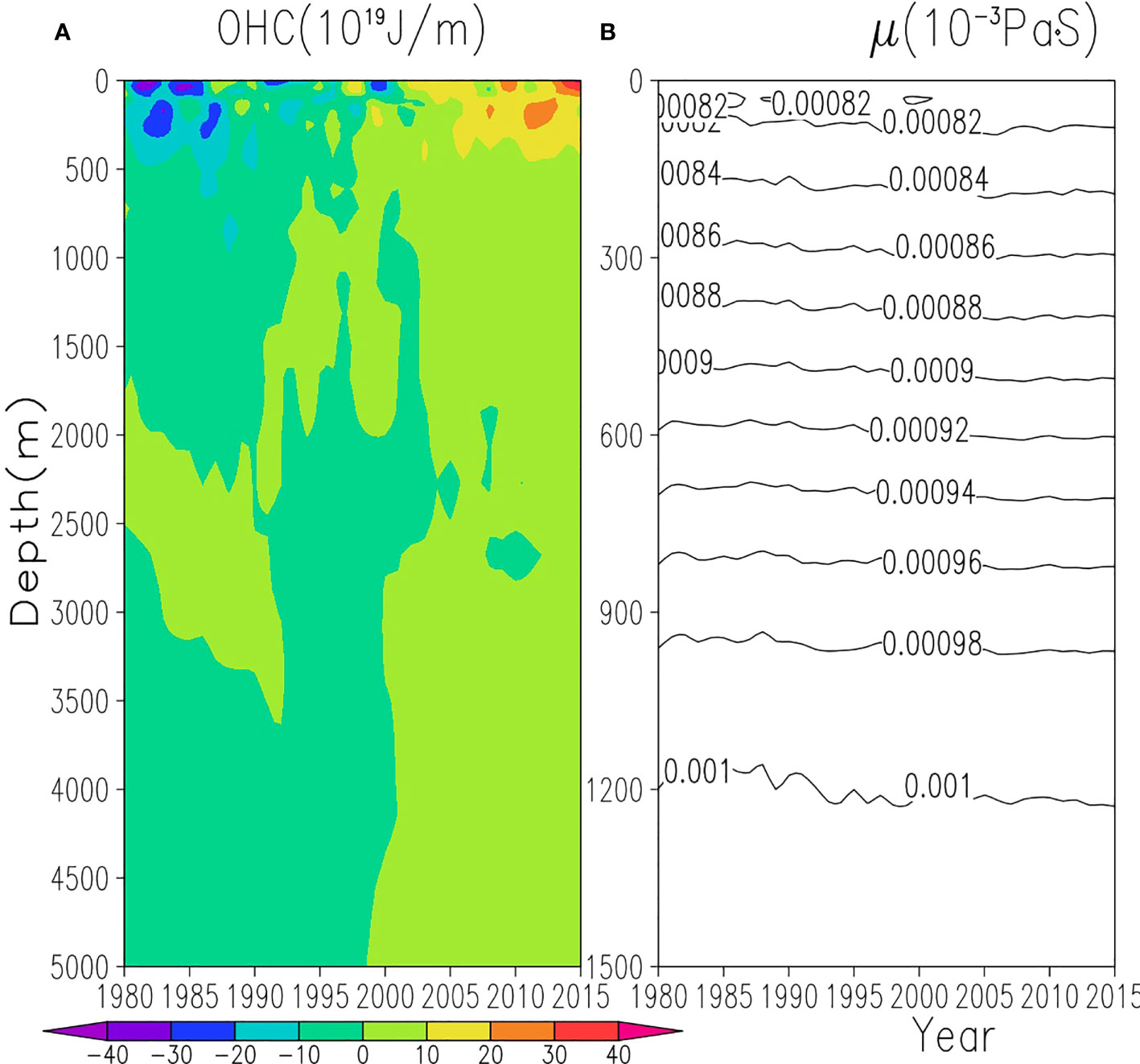
Figure 1 Increase in global oceanic heat content [up to 5,000 m, color shades, (A)] and associated reduction in viscosity [of the top 1,500-m depth, contour lines, (B)]. Data are from SODA reanalysis. In estimating OHC, the vertical resolution is 100 m. Evidently, there is a downward propagation of global oceanic heat content (overall, increase in upper 300 m is more salient than the deeper depths).

Through an oceanic conveyer belt, oceanic warming is experienced over the global oceanic basins, as seen clearly in the changes of velocity profiles of oceanic observations across the globe. Stronger oceanic currents can distribute heating to a larger region and hence deliver a milder warming rate than if the net radiation input was confined to a smaller domain. Similarly, weak oceanic circulation leads to heat buildup regionally, with consequences of extreme weather. By analyzing the oceanic energetics using reanalysis data, this study examines the root cause of the observed oceanic circulation slowing down and answers whether or not it persists as climate warms.

Similar to the atmosphere whose kinetic energy is concentrated in jet streams, the OKE is very unevenly distributed in the global oceans (Figure 2), with over 90% concentrated in major ocean currents. Here, we will examine the global total (180°W–180°E, 75°S–90°N) ocean kinetic energy as well as the following four major currents: the North Pacific drift (NP; 100°E–220°E, 20°N–40°N), the North Atlantic currents (NAC; 80°W–40°W, 45°N–60°N), the Equatorial currents (EC; 100°E–60°W, 10°S–10°N), and the Antarctic Circumpolar current (ACC; 0°E–60°W, 65°S–35°S). Their respective geographical extent is defined with lines of different styles in Figure 2. From Figures 1, 3, OHC for the entire ocean (Figures 1A, 3A) and the upper 200 m (Figure 3B) steadily increases from 1980 (the dataset starting point; in reality, the increase may have started even earlier). The global ocean heat content (0- to 200-m depth) has increased at a rate of ~11 × 10²¹ J/yr, ranging from 8 ×10²¹ to 18 × 10²¹ J/yr if examined at finer temporal scales. The two major contributors are the North Atlantic and the southern oceans (Figure 4B). In contrast, the apparent OKE decrease started late 1990s with a relatively stable period (1980–2000) followed by a steady decrease from 2000 onward, a signal consistent at all depths. Further investigation (see Figure 4A) indicates that the Atlantic Ocean has contributed the most to the decline of OKE; ostensibly, this was due to the OKE associated with the AMOC (Collins et al., 2013; Rahmstorf et al., 2015). To date, the OKE has no apparent trend in the ACC region (a test for the trend failed a t-test with a p-value > 0.05).

FIGURE 2

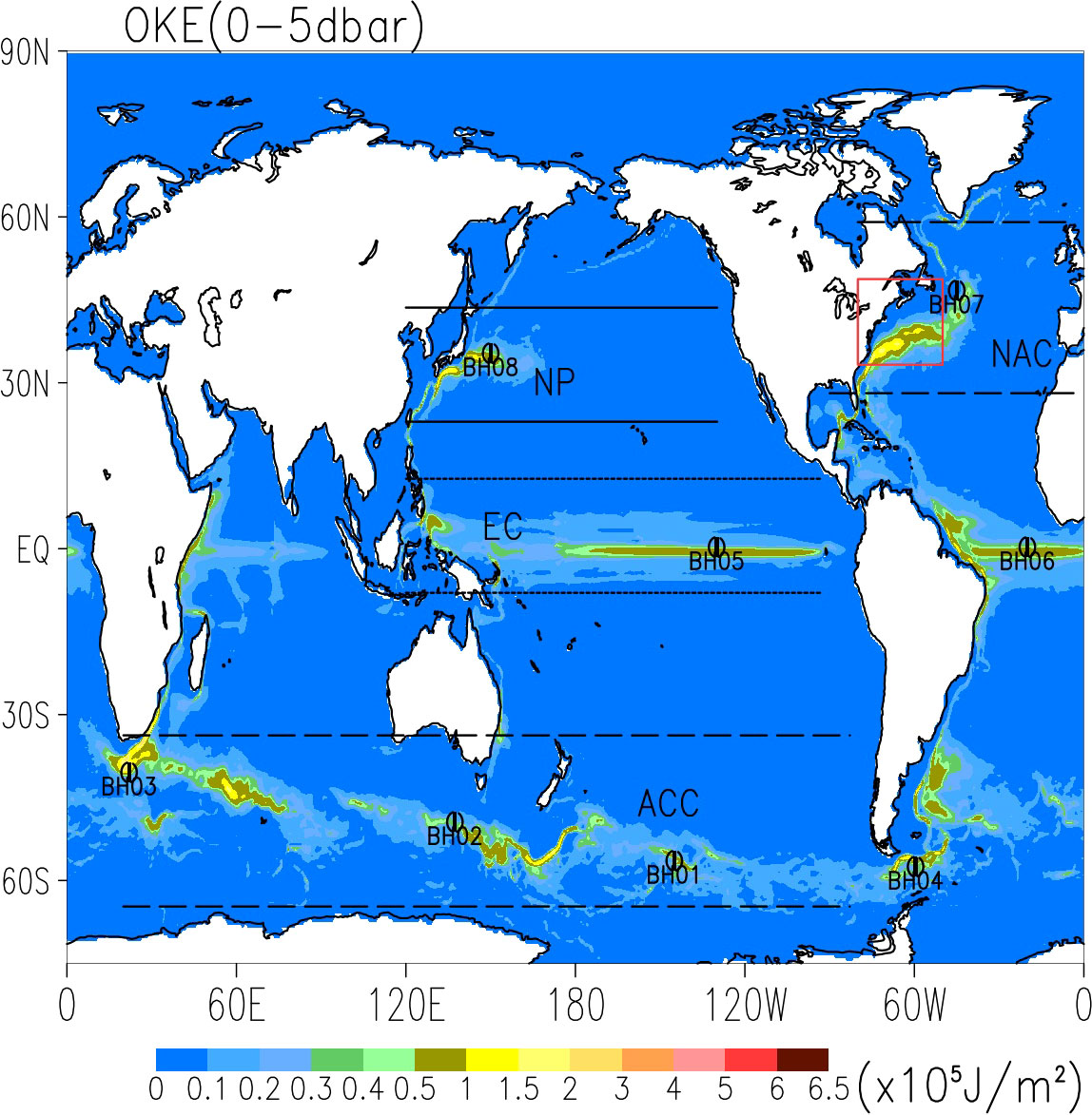
Figure 2 Global kinetic energy density (energy in an oceanic column of unit surface area). Currents and sampling locations for velocity profiles (boreholes 0–8) are labeled. Geological oceanic ranges of the North Pacific drift (NP), North Atlantic currents (NAC), Equatorial currents (EC), and Antarctic Circumpolar current (ACC) are defined with lines of different styles. Other mention of basins in the text is conventional. Boreholes are labeled with markers with a vertical bar. Red box defines the Gulf Stream region discussed here (30°N–45°N, 80°W–50°W).

FIGURE 3

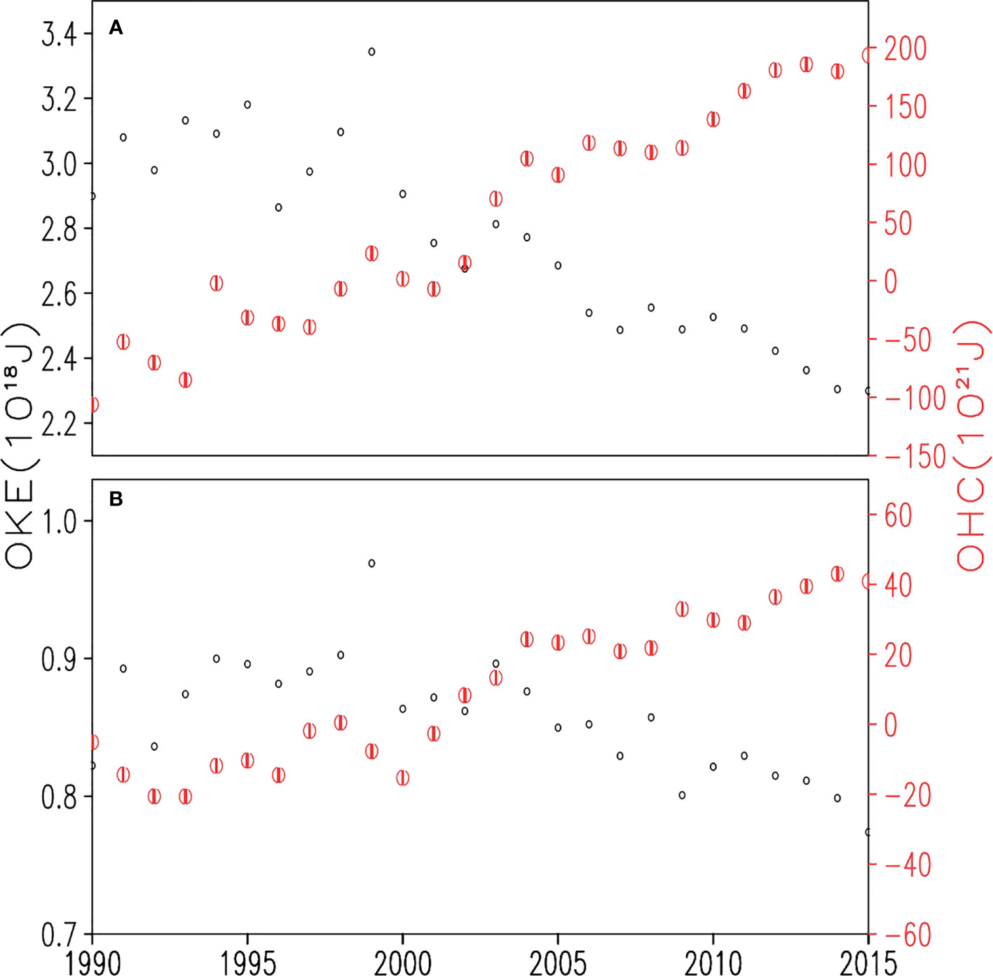
Figure 3 Evolution of oceanic kinetic energy (OKE; unfilled black dots) and heat content (OHC; red marker with a vertical bar, secondary vertical axis) for the entire ocean (A) and the upper 200 m (B). At each grid point, the reference temperature is the long-term mean (1980–2015) temperature value.

FIGURE 4

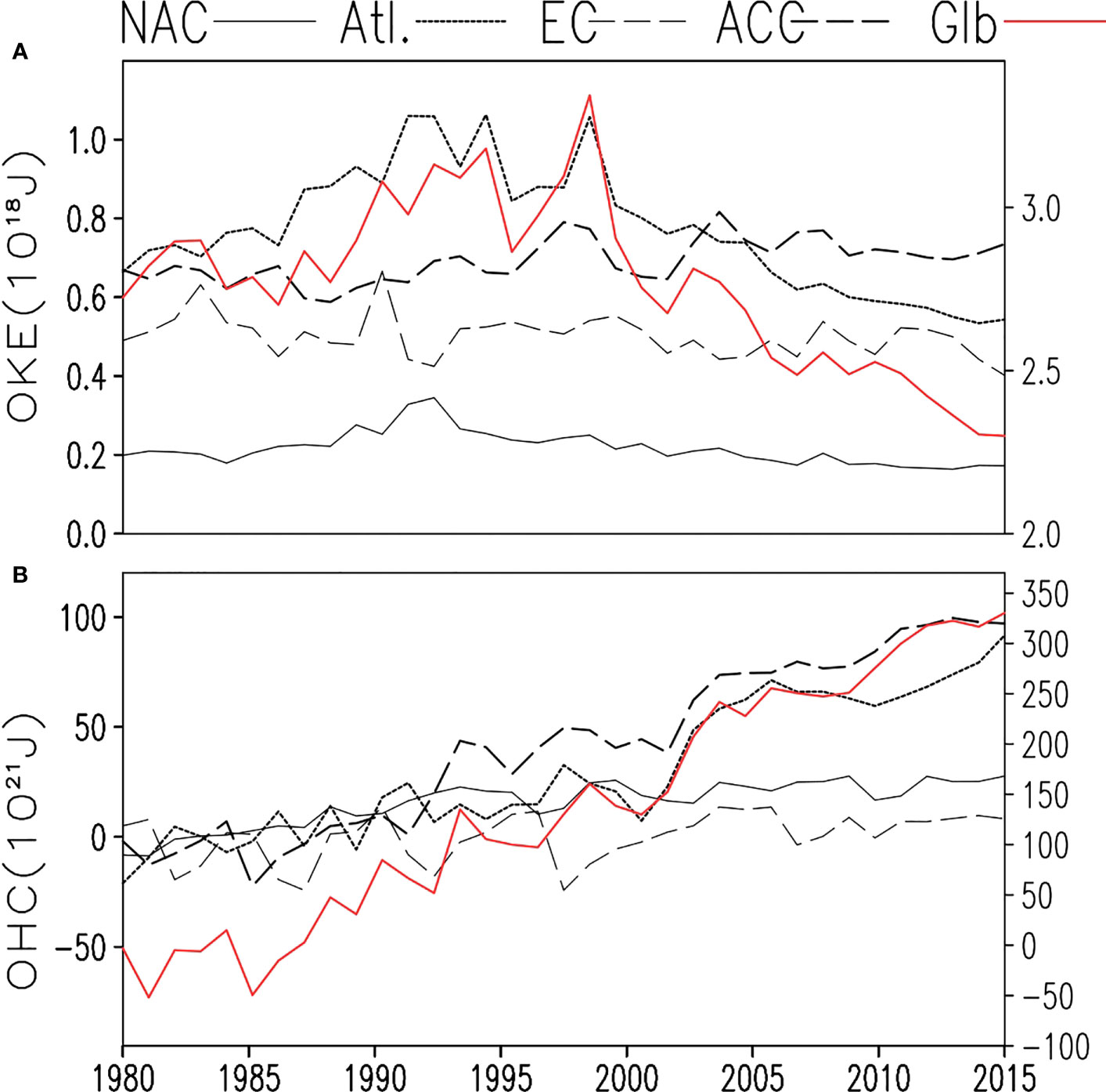
Figure 4 Time series of column total kinetic energy (A) and oceanic heat content (B) over four selected basins [Atlantic basin (Atl; 100°W–10°W, 55°S–65°N), the North Atlantic currents (NAC; 80°W–40°W, 45°N–60°N), the Equatorial currents (EC; 100°E–60°W, 10°S–10°N), and the Antarctic Circumpolar current (ACC; 0°E–60°W, 65°S–35°S)] and the entire globe (secondary vertical axis).

As the global mean OKE varies differently before and after 2000, we define 1980–2000 as Phase I of the oceanic warming and 2001–2015 as Phase II. For Phase I, the polar amplification effect (e.g., Budyko, 1969; Manabe and Wetherald, 1975; Hansen et al., 1984; Ren, 2010) is becoming dominant, and the wind stress does not apparently decrease with warming, owing to the increased near surface air viscosity over the ocean. Thus, a weakening of winds in the boundary layer does not necessarily imply a reduced wind stress over the ocean in this period. After 2000, the ocean warming enters a new phase, and the decreased oceanic viscosity becomes more and more important. At this phase, the warming of the ocean has spread to a sizable depth, and the simultaneous reduction in viscosity weakens the vertical linkage (manifested as the increased vertical velocity shear) and overall weakened ocean currents (reflected in the decreased total kinetic energy). In the overall global air–sea interaction, the combined effects of atmospheric viscosity (increased) and wind speed (reduced) produce an effective net reduction in wind stress that slows down the ocean currents.

Regionally, there are apparent phase delays. For example, the polar amplification effects over the ACC still are not significant. On the contrary, the wind stress increase started in 1993 and likely was attributable to the southward displacement and intensification of the circumpolar jet, due largely to the radiative feedback from the healing of the Antarctic ozone hole (e.g., Thompson and Solomon, 2002). The increase in KE counteracts the warming of ocean-caused viscosity decrease and, hence, a weaker link among vertical layers (reduction of OKE). That explains the lack of a trend, thus far, in OKE over the ACC region. Analysis of the SODA data supports the idea that the balance of mechanical energy is the key to maintaining deep ocean circulation, although it is clear that the ongoing climate change has reduced the ocean surface wind speeds, resulting primarily from the reduced meridional temperature gradient from polar amplification (and, hence, weakened polar jet streams). The external source of mechanical energy or the wind stress does not decrease immediately because of the compensating effects from the increased air viscosity (Ren et al., 2020). Only as warming continues (after ~2010) does the surface stress experience a net reduction. This phase delay partly explains the reported hiatus in climate warming. The weather reality is a combination of (undulating) natural variability and (steady) anthropogenic warming. When the two are out of phase, the warming signal may be hidden. When the warming effects are accumulated to a certain degree, natural variability likely can no longer reverse the trend and completely hiding the warming trend. Considering the lager heat capacity of oceans, the turning point of OKE at year 2010 (except ACC) has significant consequences in easing future warming hiatus. Consequently, more frequent winter storms in lower latitudes and more frequent heat waves in extratropical areas, as a result of outbreak of polar vortex (e.g., Kohyama et al., 2021), may become a new normal. The poleward energy transport is a relay of the atmospheric circulation and the oceanic currents. Enhancement of the atmospheric component compensates the weakened oceanic energy transport capability.

Year 2010 is a critical point for natural variability that can also be revealed by examining large-scale, inter-basin thermal contrasts. The tropical interactions between the Atlantic and Indian Oceans with the Pacific Ocean changed in the late 1990s (Han et al., 2014; Cai et al., 2019). For example, the Interdecadal Pacific Oscillation (IPO; Meehl et al., 2011) phase transition at the turn of this century has led to an unprecedented acceleration of the Walker circulation. Consequently, the associated increase in wind-stress curl has enhanced ocean heat uptake (Meehl et al., 2011). The enhanced Walker circulation also intensifies the Indonesian Throughflow (ITF; Sprintall et al., 2014). The increased heat uptake in the Pacific was partly transported to the Indian Ocean through ITF. Because the temperature threshold for deep convection increases with the mean tropical temperature (Johnson and Xie, 2010), the relative warming can be represented by a tropical Indian-minus-Pacific trans-basin SST gradient, referred to as trans-basin variability (TBV), to remove the mean tropical warming. TBV can also be similarly defined for the Atlantic Ocean basin versus the Pacific Ocean basin (Figure 5). Year 2010 is the peak time of basin-wide thermal contrast. Both Indian and Atlantic TBVs, through a Gill-type response in the atmosphere and an oceanic Bjerknes feedback, led to a La Nina–like state in the Pacific (McGregor et al., 2014; Li et al., 2016). Through these mechanisms, the deep convective activity over tropical Pacific has been suppressed for the past ~20 years. From Figure 5, the IPO appears about to enter a positive phase, and, with that, the deep convection over the Pacific basin may again increase soon.

FIGURE 5

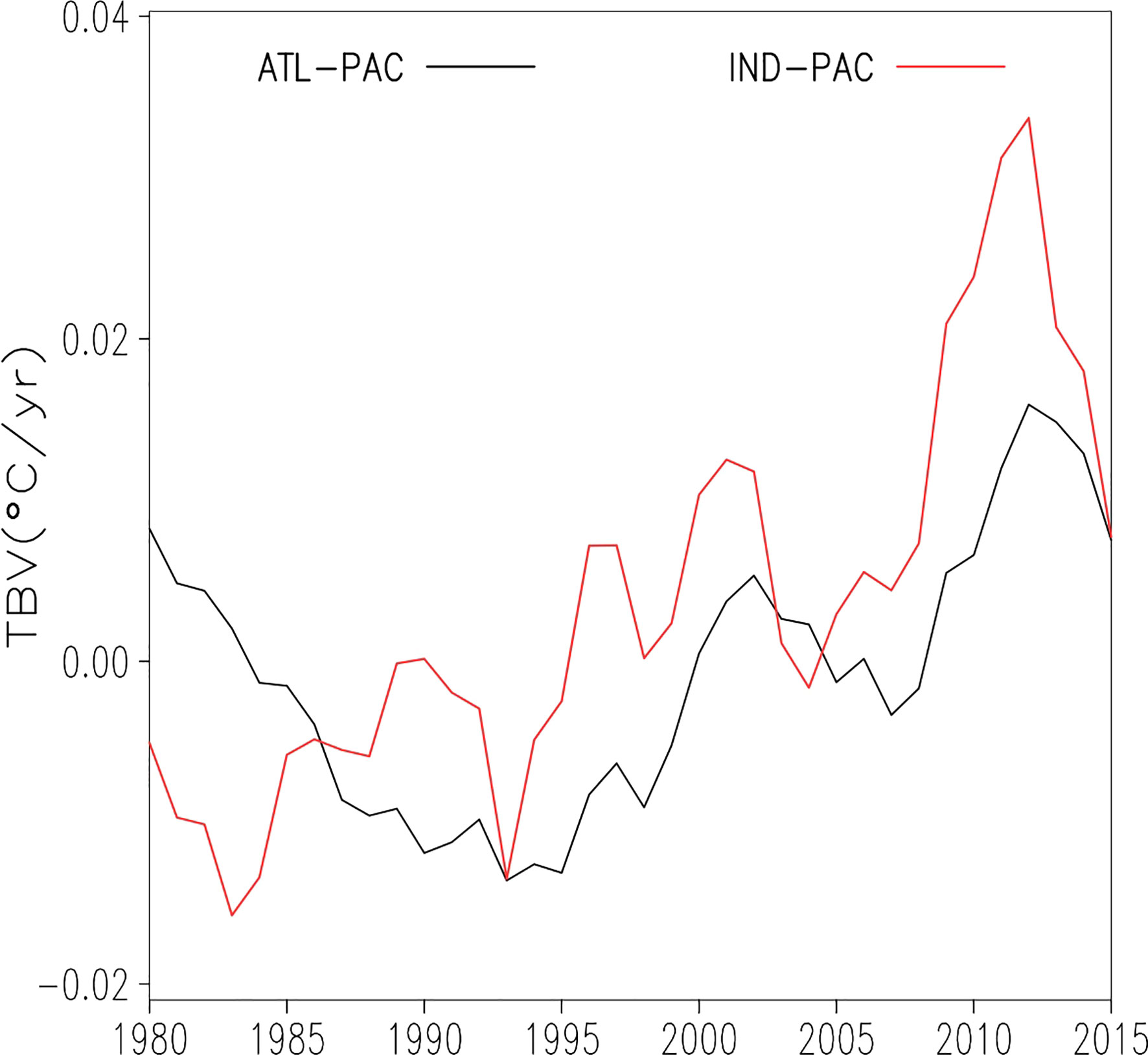
Figure 5 Sliding-window of 20-year trends of inter-basin SST differences [trans-basin variability (TBV)] for Atlantic-minus-Pacific trans-basin SST gradient (ATL-PAC) and Indian-minus-Pacific TBV (IND-PAC). SST is from the Extended Reconstructed Sea Surface Temperature (ERSST). Indian (IND), Pacific (PAC), and Atlantic (ATL) basin SST are calculated between 20°S and 20°N, respectively, for longitudinal ranges of 21°E–120°E, 121°E–90°W, and 70°W–20°E.

Reduced viscosity implied also a reduced internal friction (a mechanism transferring OKE to OHC), or, less KE is used to warm up the ocean. To examine whether that is a significant contributor to OHC fluctuation, Figure 6 shows the evolution of OKE and its viscous dissipation rate for the entire ocean depth over gulf stream (35°N–45°N, 80°W–40°W, an area of ~5.7 × 10⁶ km², as defined in Figure 2), during 1990–2015. The accumulative viscous dissipation of OKE is ~8.4 × 10¹⁵ J, four orders smaller than the increase in OHC during this period (4 × 10²⁰ J). Hence, reduced internal friction is insignificant for the change of OHC, compared to the net radiative imbalance and extra sensible heat flux from the atmosphere. Reduced eddy viscosity primarily manifests as a weaker vertical link of flow regimes and a tendency to reduce the mixing layer depth (to be detailed later). As a result, heat is concentrated in a shallower upper level of waters, contributing to enhanced vapor provision to atmosphere and favoring extreme precipitations of the related weather system such as tropical cyclones. This is confirmed further from examining the heating pattern of the oceans. For example, because of the strong temperature advection, the increased OHC can reach as deep as 2,500 m to the north of 45°N portion of the Gulf Stream (Figure 7). South of the 42°N, the most salient warming is the shallower 300 m of mixed layer. The top 200-m water warmed up by ~0.3°C for the 35°N–45°N section during the reanalysis period. Comparing the periods 1980–2000 and 2000–2015, the shallower levels warm up much saliently than deep levels, in a pattern more concentrated than explainable from a temperature-invariant eddy viscosity. This supports Meehl et al. (2011) in ascribing hiatus in near surface warming to a reduced heat storage capacity of shallower (<300 m) ocean water. From this viscosity-caused positive feedback in reducing oceanic heat storage capacity, the hiatus likely is transient. Even if the net radiative imbalance holds at 1 W/m², the steady decrease of oceanic viscosity tends to store the extra heat in an ever-smaller space close to surface. This likely terminate the hiatus in warming before 2060, from examining the same data as reported by Meehl et al. (2011). In case the stronger business-as-usual emission scenarios are realized, the timing of anthropogenic warming permanently dominating over natural variability could be as early as 2030. From that point onward, a weakened poleward transport of heat by the THC would be a new normal. Consequently, the atmosphere has to take over more share in the longitudinal energy and momentum transfer (Bjerknes compensation effect; Bjerknes, 1964; Shaffrey and Sutton, 2006). Adjusting to the changed thermal contrasts and enhanced hydrological cycle, outbreak of polar vortex (weakened polar jets; Ren et al., 2020) and more watery hurricanes (with higher than normal along track precipitation) would follow, among others.

FIGURE 6

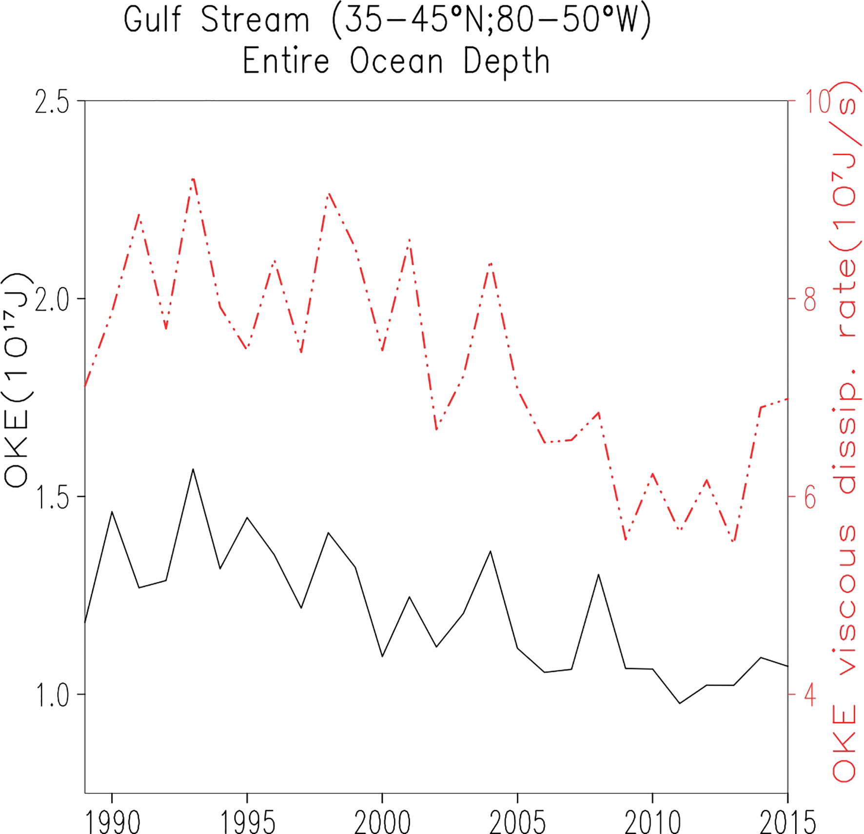
Figure 6 Evolution of oceanic kinetic energy (black line) and its viscous dissipation rate (red line) for the entire ocean depth over gulf stream, during 1990–2015.

FIGURE 7

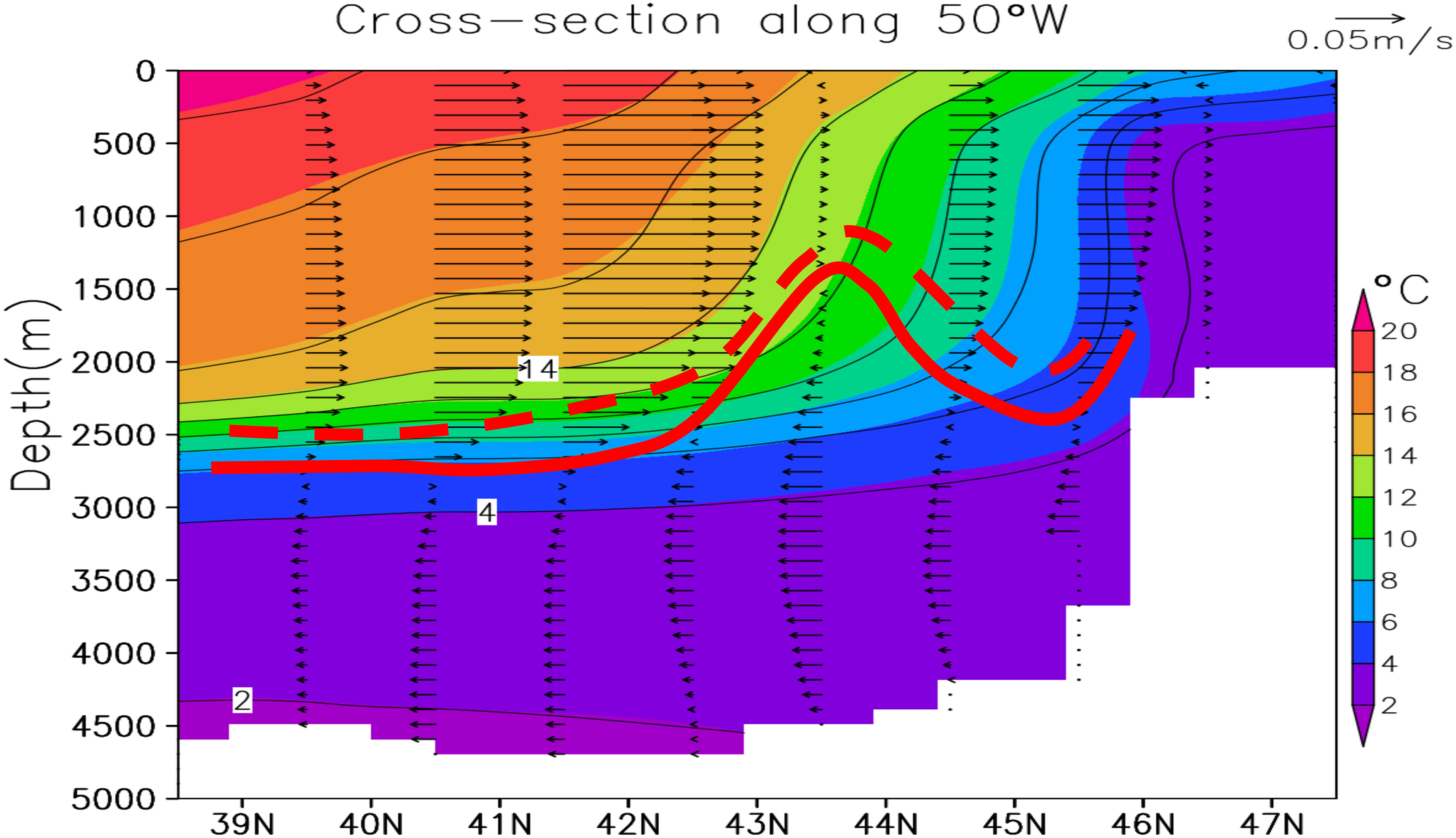
Figure 7 Ocean states along a 50°W segment off the Labrador Sea. Vectors are meridional (v-component) component of the ocean flow. The flow reverse level is marked with a thick red line. This surface was lifted by over 200 m over the period (1980–1990) to (2000–2015). Color shades are potential temperatures over the (1980–1990) period. Black contour lines are potential temperatures over the (2000–2015) period.

Over the entire reanalysis period, the downward propagation of OHC is a globally consistent phenomenon (Figure 2). The viscosity reduction in the upper 1500 m of the ocean is shown for the globe and for the representative basins (not shown for clarity). On the basis of the SODA reanalysis data, the deepest, smoothed basin is 5,000-m deep. The global OHC increase is partitioned among the various ocean basins. The Pacific and Indian Oceans dominate the horizontal exchange of heat in the upper 250 m (Lee et al., 2015; Nieves et al., 2015), and the Atlantic and the Southern Oceans dominate the vertical redistribution, evident in the drastically different vertical profiles of the flow speeds (Figure 8). The prevailing Couette oceanic flow is often tinted, to various extents, with Poiseuille features, arising from either uneven salinity distributions or various types of coupling between bathymetry and prevailing surface wind stresses. For example, a rising elevation in the direction of the surface winds may distort the flow profile, thereby generating counter currents. Close to the lateral boundaries and the ocean floor, the importance of secondary flows increases, as does the randomness associated with the turbulence. To reveal persistent changes in the flow structure induced by viscosity changes, averaging over an extended period is necessary to filter out short-term noise present in the reanalysis data. The velocity profiles in Figure 8 are long-term means of March profiles over two periods: 1980–1994 and 2001–2015. Their profiles are very different, primarily due to the local matching of dominant wind stress and bathymetry at specific “borehole” locations. For all of the boreholes, the vertical gradients of the flow profiles are larger during the 2001–2015 period. This is especially apparent in the top 1,500 m, evidently due to the reduced viscosity. These eight boreholes are representative of the global oceans, and the steepening of the velocity profiles is now a global phenomenon. Here, we stress the temperature contribution to the reduced viscosity because it is a global phenomenon. The contribution to a reduced viscosity also arises because of the freshwater discharge from the polar icesheets and ice shelves. This process is apparent from the reanalysis salinity changes over the region (figure not shown). Using SEGMENT-Ice–simulated ice shedding rates (Ren et al., 2021) and the high-resolution Geophysical Fluid Dynamics Laboratory (GFDL) model–simulated flow structure, the freshwater discharge of ~170 Gt/yr from the Greenland Ice Sheet to the north Atlantic basin (present day situation) corresponds to a 0.3% reduction in viscosity of the top 300-m depth for the regions north of 55°N.

FIGURE 8

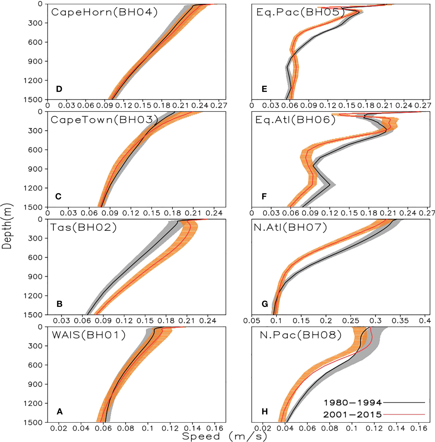
Figure 8 Mean March ocean speed profiles at eight different oceanic locations (A–H), for two periods: 1980–1994 (black lines) and 2001–2015 (red lines). Horizontal bars are standard deviations at different depths, calculated from monthly data from the two 15-year periods of the SODA reanalysis data. The vertical shear increased for all these places, a shared feature indicating a reduced viscosity. Measurements cannot differentiate wind-stress driven or thermohaline driven currents. However, it is clearer that the Couette feature, if it exists, is more salient closer to the surface.

It is noticeable that the mixed layer currents of BH05 and BH06 also have weakened slightly or, at least, are not being enhanced by the expansion of the subtropical highs (Ren and Leslie, 2015, and references therein). In the lower troposphere, ongoing polar amplification is weakening the meridional temperature gradient. In contrast, in the upper troposphere and lower stratosphere, the meridional temperature gradient is strengthening because of the combined effects of polar lower-stratospheric cooling and tropical upper-tropospheric warming. The latter is the consequence of water vapor feedback releasing additional latent heat and reducing the temperature lapse rate. Thus, the vertically integrated thermal wind response to warming is a contest between two competing effects. The wind speeds surrounding the subtropical highs become stronger at upper levels. At the sea level, the subtropical high covers a larger area but with an overall reduction in wind speeds (figure not shown). This also explains the observed SST synchronization of the Gulf Stream and the Kuroshio Current by the polar jets, on decadal time scales (Kohyama et al., 2021).

Analysis of ERA5 data confirmed that the lower troposphere polar amplification, which is dominated by lower-boundary forcing and feedbacks, is weakening the meridional temperature gradient (Ren, 2010) and the polar jet stream (Francis and Vavrus, 2012; Haarsma et al., 2013). This partially contributes to the weakening of the AMOC and the North Pacific currents in the Northern Hemisphere. Because, except for the West Antarctic Peninsula, the pristine Antarctica is still covered by solid ice all year round (hence, there is no salient albedo changes), and, because the mid-latitudes of the Southern Hemisphere are dominated by oceans, polar amplification is not yet apparent. The subsurface Southern Ocean has been warming since, at least, 1993 (Figure 4B). Because of the southward displacement and intensification of the westerly jet (figs not shown here for brevity), its kinetic energy also is increasing (Figure 4A). However, this trend of shifting and intensification cannot continue much longer due to two reasons: first, because the proposed cause (the ozone hole) has diminished in importance with the healing of the ozone hole (still ongoing); second, there is not much more room for the jet’s further southward displacement. We estimate that, with the reduction of the Antarctic ozone hole and the possible onset of southern polar amplification (likely starting from the Drake passage region), it is anticipated that ACC over the Southern Oceans will slow down since ~2050. The very shallow portion likely will not slacken because of the reduced oceanic viscosity. However, both the vertical linkage and the overall flow of the subsurface layer are expected to weaken. For the primarily wind-driven currents (e.g., Figure 8C), the reduction will dominate in the upcoming decades as the warming continues. With atmospheric parameters from ensemble climate model simulations under a strong emission scenario (the business-as-usual Representative Concentration Pathway 8.5 Watts per Square meter), the SEGMENT-Ice, with ice-sheet basal mechanisms and marine terminating ice instability implemented (Ren and Leslie, 2011), indicates that ice creeping is accelerating over West Antarctica, especially along the Amundsen Sea coast. Polar amplification over southern hemisphere will not be limited to the type of traditional albedo feedback (from ocean color changes and sea ice variations), ocean–land ice interactions will play a significant role. Among them, the freshening sea water at the ice shelf (and ocean-terminating glaciers) possesses higher capability in further eroding solid ice deserves further investigation, because it is a positive feedback mechanism that further reduces the oceanic viscosity. The turning timing of 2050 for ACC is determined here on the basis of the overall healing of the ozone hole under the Montreal Protocol (signed in 1978). There is also hiatus in the healing process, due to (natural) interannual variability of meteorological and dynamical conditions that can have an important impact on the magnitude of the ozone hole fluctuations and are superimposed on the long-term recovery. Strictly implementation of the Montreal Protocol means a steady no–ozone hole condition around 2030. However, because of the natural variability, it will take about three more decades for the ozone layer to fully recover. Because of its unique nexus role in connecting the major oceans (i.e., the Southern Ocean is the upwelling region of the dominant ocean currents; the ice–air–ocean interactions are complex; and the atmospheric circulation above is unique), the ACC is a central component of the global ocean heat uptake and storage in a warming climate (e.g., Sallee, 2018, and references therein). Air–sea interactions, for example, mechanisms associated with wind changes, and ocean–ice interactions remain areas of active research. The sensitivity of oceanic viscosity to warming is one aspect that was so far overlooked but apparently deserves more attention.

For the northward marching of the Gulf Stream, the vigorous evaporation and the associated cooling of the (near) surface ocean water is critical for the development of the sinking branch of the AMOC and the maintenance of the strength of the returning deep water flow. North of ~50°N, saltier, heavier water generally overlays fresher water, forming an inverse distribution of viscosity (Figure 9A). Even within the descending branch, the descending slope is very gentle, so the kinetic energy of the currents still is dominated by the horizontal flow components. As a characteristic THC, the wind stress reduction accounts for only a fraction of the reduced strength of the AMOC. Freshwater discharge (e.g., from the GrIS) reduces the buoyancy driving force while it also reduces the kinematic viscosity (Figure 9). These two effects work in synergy to reduce the total kinetic energy associated with the conveyor belt because the involved total water volume (and the mass) reduces—the thickness of the water in motion is reduced as the velocity profile develops steeper gradients. During the reanalysis period, even as the OHC increases steadily over the global oceans, global winds have significant phase shifts in response to warming. Consequently, the kinetic energy reduction starts very differently, with the North Atlantic Ocean starting as late as around 2000 (Figure 4A).

FIGURE 9

Figure 9 Reduction in kinematic viscosity over 1980–2015 for four oceanic basins: (A) for AMOC sinking region (NAC), (B) for NP, (C) for ACC, and (D) for global.

The slowing down of the AMOC has been noted from observations since 2004 from the time series of the RAPID array, which shows the flow discharge rate along the 26.5°N latitude (Smeed et al., 2018). Climate models also project a gradual slowing of the AMOC over the 21st Century, in response to anthropogenic forcing (e.g., Weaver et al., 2012; Trenberth and Fasullo, 2017). A more complete review of the slowing AMOC is provided by Weijer et al. (2019). Thus, it is a significant climate consensus that the slowing down of AMOC under global warming is well established. However, there is some disagreement about whether the slowing will continue and, hence, transform the ocean circulation into another state, given that the AMOC has multiple stable and critical states (e.g., Rahmstorf, 1995; Guan and Huang, 2008, and references therein). The transitioning between the several stable states is internally linked by the viscosity. From our above discussion, the interactions of climate warming and ocean currents are centered on eddy viscosity’s sensitivity to temperature changes. As illustrated in Figure 10, the shallower-depth Couette profiles (red curves) have salinity gradient–driven Poiseuille bulges superimposed upon them. The returning Poiseuille profiles are further modified by bottom bathymetry. In a warmer climate, the flow profiles will be confined tightly, with reduced total kinetic energy. Consequently, the stagnant mixed layer may shift upward and shrink in total volume. This indicates a reduced heat storage capability of the oceanic mixed layer in the transient climate change period. Detailed properties of flow may vary, but the generic feature holds. Recently reported slowing down of the AMOC, with it its weakened poleward transportation capability, and concentrated heat storage in the shallower mixed layer (that spawns sustained precipitation systems such as hurricanes) agree with this hypothesis (Muschitiello et al., 2019).

FIGURE 10

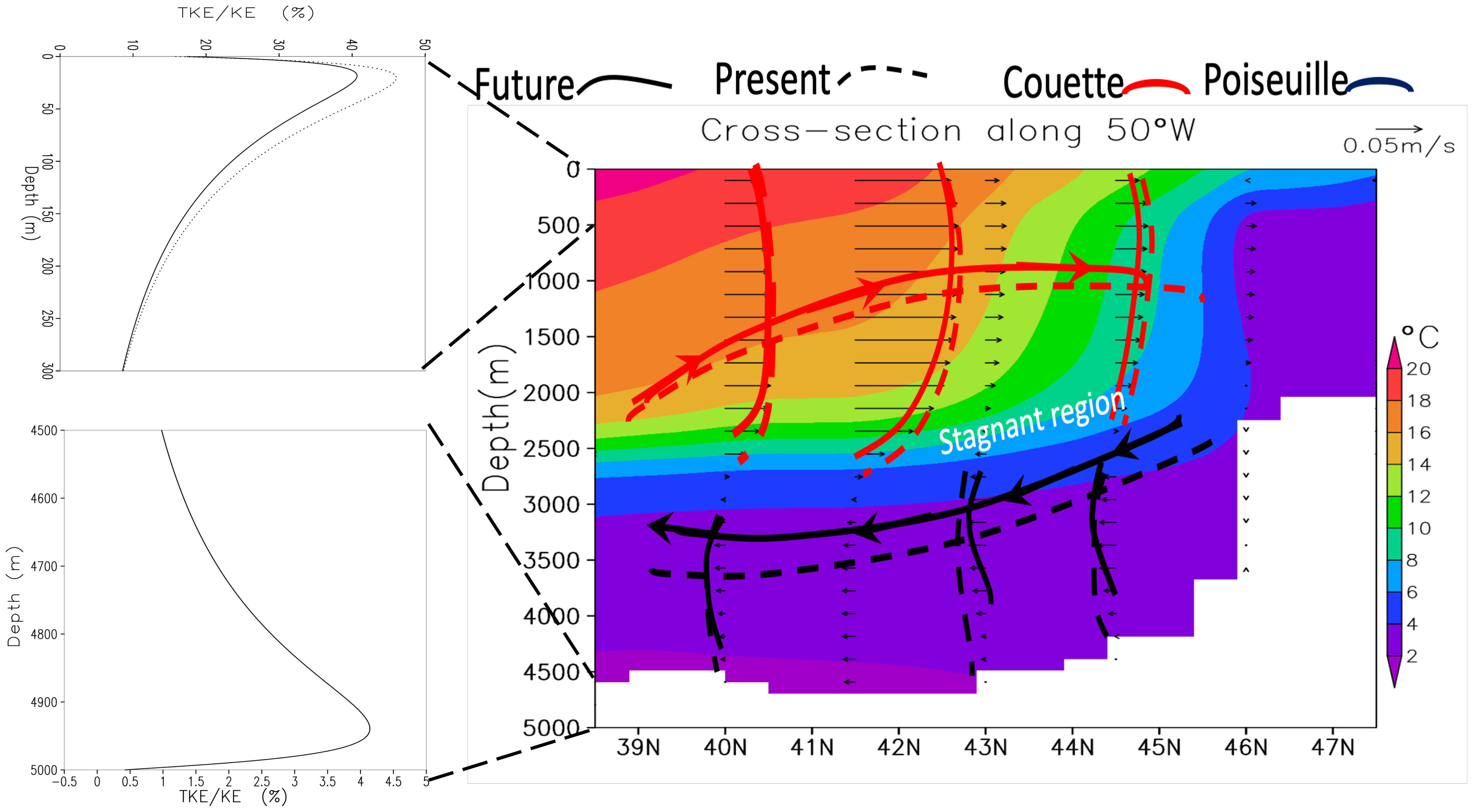
Figure 10 Illustration of a weakened oceanic conveyor belt. Transect along the 50°W. Red lines with arrows signify the median level of upper (poleward advancing) currents, and black arrow lines signify the median levels of the lower (returning) flow. Dashed lines for present climate, and solid lines for a warming climate. Shades are potential temperature in degree Celsius. Drivers of oceanic flow can be surface wind stress (Couette flow) and thermohaline (Poiseuille flow). Bottom topography itself does not contribute to flow, but various coupling of bathymetry with surface wind stress alter flow regimes. Consequently, the basic Couette–Poiseuille flow structure can be distorted to the extent that it may generate secondary and even inverse flows. According to a Reynolds number–dependent dissipation rate scheme (e.g., Mellor and Yamada, 1982), the turbulent kinetic energy’s (TKE) proportion of total OKE is illustrated as zoom-in panels to the left. As warming continues, the reduction of the upper “boundary layer” is apparent. The bottom, bathymetry-caused TKE is of much reduced magnitude and do not significantly change with warming on the near term.

4 Discussions and conclusions

This article surveys current progress and the outlook for atmospheric–oceanic coupled system energetics, including the downward energy cascade, in physical contexts. It also explains the observed facts of the oceanic circulation and answers whether the weakening of the oceanic circulation should be expected to persist, by examining the nexus role played by the temperature-dependent eddy viscosity. Global warming has reached a stage where the accumulated effects from polar amplification have substantially reduced the wind stress over the subpolar gyres. The consequences are weakened circulations over the Indian and Pacific oceans, especially for the North Pacific Drift. The same effects are applied to the Gulf Stream but are superimposed on the AMOC. The thermohaline catastrophe implied in Stommel (1961) and confirmed by numerical models (e.g., Bryan, 1986; Manabe and Stouffer, 1988; Cubash et al., 1992) is now clearly seen in the reanalysis data and in an even more generic expression of the circulation slowing down. In the recent decades, the net top of atmosphere energy imbalance of ~1 W m⁻² is the propagator of the inexorable climate warming. How the energy surplus is partitioned has practical implications for extreme-weather–related natural hazards mitigation (Ren, 2014; Ren and Leslie, 2020). The observed OKE trend from 1980 cannot be explained by changes in surface winds alone but can be explained satisfactorily by also taking into consideration the temperature dependence of atmospheric and oceanic viscosity. Warming and freshening of the ocean can lower the ocean viscosity and reduce the vertical linkage in oceanic motion and, consequently, lead to a reduction of the total OKE. This trend was not clear before 1990 because the wind stress reduction is counteracted by an increase in air viscosity associated with a warming climate (Ren et al., 2020).

The reduction in oceanic circulation from global warming will continue but, fortunately, at an ever-decreasing rate. Its direct manifestation will be an accelerated near-surface oceanic warming in the upcoming decades. Reduced viscosity signifies a reduced mixing layer depth. Consequently, net radiative imbalance and sensible heat flux excess due to a warming atmosphere will be concentrated in a shallower upper level of waters—a configuration enhancing vapor provision to atmosphere and favoring extreme precipitations of the related weather systems. Temperature-dependent viscosity not only reconciles previous climate model simulations of the weakening of the THC [e.g., the assertation of Manabe and Stouffer (1993), a transient behavior for a CO₂ doubling and a permanent feature for quadrupled atmospheric CO₂ concentrations; or stronger vs. weaker net radiative balances] but also indicates that, with the persistent reduction of oceanic viscosity, heating of the shallower ocean will get more intense. The resulted weaker oceanic heat transport will be compensated by atmospheric branch of circulation by taking more latent heat.

In summary, our analysis indicates that the temperature-dependent viscosity should be included in the state-of-art climate models for us to better understand how the climate system will respond to the greenhouse gas induced warming. Although studies have suggested that the ocean mixed layer is shoaling under a warmer climate (Capotondi et al., 2012), the lowering of the sea water viscosity may have made this shoaling more serious and lead to a more intensified surface warming.

Data availability statement

The original contributions presented in the study are included in the article/supplementary material. Further inquiries can be directed to the corresponding author.

Author contributions

DR: Initiated the study and wrote the paper together with co-author. AH: Wrote the paper and carried out part of the research. Both authors contributed to the article and approved the submitted version.

Acknowledgments

Portions of this study were supported by the Regional and Global Model Analysis (RGMA) component of the Earth and Environmental System Modeling Program of the U.S. Department of Energy’s Office of Biological and Environmental Research (BER) via National Science Foundation (IA 1844590). National Center for Atmospheric Research is sponsored by National Science Foundation of the United States of America.

Conflict of interest

The authors declare that the research was conducted in the absence of any commercial or financial relationships that could be construed as a potential conflict of interest.

Publisher’s note

All claims expressed in this article are solely those of the authors and do not necessarily represent those of their affiliated organizations, or those of the publisher, the editors and the reviewers. Any product that may be evaluated in this article, or claim that may be made by its manufacturer, is not guaranteed or endorsed by the publisher.

References

Bjerknes J. (1964). Atlantic air–sea interaction. Adv. Geophysics 10, 1–82. doi: 10.1016/S0065-2687(08)60005-9

CrossRef Full Text | Google Scholar

Brown R., Liu W. (1982). An operational large-scale marine planetary boundary layer model. J. Appl. Meteorol. 21, 261–269. doi: 10.1175/1520-0450(1982)021<0261:AOLSMP>2.0.CO;2

CrossRef Full Text | Google Scholar

Bryan F. (1986). High latitude salinity effects and interhemispheric thermohaline circulations. Nature 323, 301–304. doi: 10.1038/323301a0

CrossRef Full Text | Google Scholar

Budyko M. (1969). The effect of solar radiation variations on the climate of the Earth. Tellus 21 (5), 611–619. doi: 10.3402/tellusa.v21i5.10109

CrossRef Full Text | Google Scholar

Cai W., Wu L., Lengaigne M., Li T., McGregor S., Kug J., et al. (2019). Pantropical climate interactions. Science 363, eaav4236. doi: 10.1126/science.aav4236

PubMed Abstract | CrossRef Full Text | Google Scholar

Capotondi A., Alexander M., Bond N., Curchitser E., Scott J. (2012). Enhanced upper ocean stratification with climate change in the CMIP3 models. J. Geophys. Res. 117, C04031. doi: 10.1029/2011jc007409

CrossRef Full Text | Google Scholar

Carton J. A., Giese B. (2008). A reanalysis of ocean climate using Simple Ocean Data Assimilation (SODA). Mon. Wea. Rev. 136, 2999–3017. doi: 10.1175/2007MWR1978.1

CrossRef Full Text | Google Scholar

Carton J. A., Penny S. G., and Kalnay E. (2019). Temperature and salinity variability in soda3, ECCO4r3, and ORAS5 ocean reanalyses, 1993-2015, J. Climate 32, 2277–2293.

Google Scholar

Chapman S., Cowling T.. (1970). The mathematical theory of non-uniform gases (3rd ed.), .Cambridge University Press. 423.

Google Scholar

Chen X., Tung K.-K.. (2014). Varying planetary heat sink led to global warming slowdown and acceleration. Science, 345, 897–903. doi: 10.1126/science.1254937

PubMed Abstract | CrossRef Full Text | Google Scholar

Collins M., Knutti R., Arblaster J., Dufresne J. -L., Fichefet T., Friedlingstein P., et al. (2013). Chapter 12: Long-term Climate Change: Projections, Commitments and Irreversibility, in Working Group 1 Contribution to the IPCC Fifth Assessment Report Climate Change 2013: The Physical Science Basis, edited by Joussaume S., et al, 1611–1785, Cambridge Univ. Press, New York

Google Scholar

Cubash U., Hasselmann K., Hock H., Maier-Reimer E., Mikolajewicz U., Santer B., et al. (1992). Time-dependent greenhouse warming computations with a coupled oceanatmosphere model. Climate Dynamics 8, 55–69. doi: 10.1007/BF00209163

CrossRef Full Text | Google Scholar

Danabasoglu G., Bates S., Briegleb B., Jayne S., Jochum M., Large W., et al. (2012). The CCSM4 ocean component. J. Climate 25, 1361–1389. doi: 10.1175/JCLI-D-11-00091.1

CrossRef Full Text | Google Scholar

Ferrari R., McWilliams J. C., Canuto V. M., Dubovikov M. (2008). Parameterization of eddy fluxes near oceanic boundaries. J. Climate 21, 2770–2789. doi: 10.1175/2007JCLI1510.1

CrossRef Full Text | Google Scholar

Fox-Kemper B., Danabasoglu G., Ferrari R., Griffies S., Hallberg R., Holland M., et al. (2011). Parameterization of mixed layer eddies. Part III: Implementation and impact in global ocean climate simulations. Ocean Modell 39, 61–78. doi: 10.1016/j.ocemod.2010.09.002

CrossRef Full Text | Google Scholar

Fox-Kemper B., Ferrari R., Hallberg R. (2008). Parameterization of mixed layer eddies. Part I: Theory and diagnosis. J. Phys. Oceanogr. 38, 1145–1165. doi: 10.1175/2007JPO3792.1

CrossRef Full Text | Google Scholar

Francis J., Vavrus S. (2012). Evidence linking Arctic amplification to extreme weather in mid-latitudes. Geophys. Res. Lett. 39 (6), L06801. doi: 10.1029/2012GL051000

CrossRef Full Text | Google Scholar

Gent P. R., McWilliams J. C. (1990). Isopycnal mixing in ocean circulation models. J. Phys. Oceanogr. 20, 150–155. doi: 10.1175/1520-0485(1990)020<0150:IMIOCM>2.0.CO;2

CrossRef Full Text | Google Scholar

Giglio D., Johnson G. C. (2017). Middepth decadal warming and freshening in the South Atlantic. J. Geophy. Res. 122, 973–979. doi: 10.1002/2016JC012246

CrossRef Full Text | Google Scholar

Guan Y., Huang R. (2008). Stommel’s box model of thermohaline circulation revisited—The role of mechanical energy supporting mixing and the wind-driven gyration. J. Phys. Oceanogr. 38, 909–917. doi: 10.1175/2007JPO3535.1

CrossRef Full Text | Google Scholar

Haarsma R., Selten F., van Oldenborgh G. (2013). Anthropogenic changes of the thermal and zonal flow structure over Western Europe and Eastern North Atlantic in CMIP3 and CMIP5 models. Clim. Dyn. 41, 2577–2588. doi: 10.1007/s00382-013-1734-8

CrossRef Full Text | Google Scholar

Han W., Meehl G., Hu A., Alexander M., Yamagata T., Yuan D., et al. (2014). Intensification of decadal and multi-decadal sea level variability in the western tropical Pacific during recent decades. Clim. Dyn. 43, 1357–1379. doi: 10.1007/s00382-013-1951-1

CrossRef Full Text | Google Scholar

Hansen J., Nazarenko L., Ruedy R., Sato M., Willis J., Del Gemio A., et al. (2005). Earth’s energy imbalance: Confirmation and implications. Science 308, 1431–1435. doi: 10.1126/science.1110252

PubMed Abstract | CrossRef Full Text | Google Scholar

Hansen J., Lacis A., Rind D., Russell G., Stone P., Fung I., et al. (1984). “Climate sensitivity: Analysis of feedback mechanisms,” in Climate Processes and Climate Sensitivity, Geophys. Monogr, vol. 29. (Boston, USA: Amer. Geophys. Union), 130–163.

Google Scholar

Hersbach H., Bell B., Berrisford P., Hirahara S., Horanyi A., Munoz-Sabater J., et al. (2020). The ERA5 global reanalysis. Q J. R Meteorol Soc. 146, 1999–2049. doi: 10.1002/qj.3803

CrossRef Full Text | Google Scholar

Hu A., Bates S. (2018). Internal climate variability and projected future regional steric and dynamic sea level rise. Nat. Commun. 9 (1), 1068. doi: 10.1038/s41467-018-03474-8

PubMed Abstract | CrossRef Full Text | Google Scholar

Johnson N., Xie S. (2010). Changes in the sea surface temperature threshold for tropical convection. Nat. Geosci. 3, 842–845. doi: 10.1038/ngeo1008

CrossRef Full Text | Google Scholar

Kohyama T., Yamagami Y., Miura H., Kido S., Tatebe H., Watanabe M. (2021). The gulf stream and kuroshio current are synchronized. Science 374, 341–346. doi: 10.1126/science.abh3295

PubMed Abstract | CrossRef Full Text | Google Scholar

Lee S., Park W., Baringer M., Gordon A. L., Huber B., Liu Y.. (2015). Pacific origin of the abrupt increase in Indian Ocean heat content during the warming hiatus. Nature Geosci. 8, 445–449. doi: 10.1038/ngeo2438

CrossRef Full Text | Google Scholar

Lewis S., Karoly D. J. (2015). Are estimates of anthropogenic and natural influences on Australia’s extreme 2010–2012 rainfall model- dependent? Clim. Dyn. 45, 679–695. doi: 10.1007/s00382-014-2283-5

CrossRef Full Text | Google Scholar

Li X., Xie S., Gille S., Yoo C. (2016). Atlantic induced pan-tropical climate change over the past three decades. Nat. Clim. Change 6, 275–279. doi: 10.1038/nclimate2840

CrossRef Full Text | Google Scholar

Manabe S., Stouffer R. (1988). Two stable equilibria of a coupled ocean-atmosphere model. J. Climate 1, 841–866. doi: 10.1175/1520-0442(1988)001<0841:TSEOAC>2.0.CO;2

CrossRef Full Text | Google Scholar

Manabe S., Stouffer R. (1993). Century-scale effects of increased atmospheric CO₂ on the ocean-atmosphere system. Nature 364, 215–218. doi: 10.1038/364215a0

CrossRef Full Text | Google Scholar

Manabe S., Wetherald R. (1975). The effects of doubling the CO2 concentration on the climate of a general circulation model. J. Atmos. Sci. 32 (1), 3–15. doi: 10.1175/1520-0469(1975)032<0003:TEODTC>2.0.CO;2

CrossRef Full Text | Google Scholar

McGregor S., Timmermann A., Stuecker M., England M., Merrifield M., Jin F., et al. (2014). Recent Walker circulation strengthening and Pacific cooling amplified by Atlantic warming. Nat. Clim. Change 4, 888–892. doi: 10.1038/nclimate2330

CrossRef Full Text | Google Scholar

Meehl G., Arblaster J., Fasullo J., Hu A., Trenberth K. (2011). Model-based evidence of deep-ocean heat uptake during surface-temperature hiatus periods. Nat. Clim. Change 1, 360–364. doi: 10.1038/nclimate1229

CrossRef Full Text | Google Scholar

Mellor G., Yamada T. (1982). Development of a turbulence closure model for geophysical fluid problems. Rev. Geophysics Space Phys. 20 (4), 851–875. doi: 10.1029/RG020i004p00851

CrossRef Full Text | Google Scholar

Munk W. H. (1950). On the wind-driven ocean circulation. J. Meteor. 7, 79–93. doi: 10.1175/1520-0469(1950)007<0080:OTWDOC>2.0.CO;2

CrossRef Full Text | Google Scholar

Muschitiello F., D’Andrea W., Schmittner A., Heaton T., Balascio N., deRoberts N., et al. (2019). Deep-water circulation changes lead North Atlantic climate during deglaciation. Nat. Commun. 10, 1272. doi: 10.1038/s41467-019-09237-3

PubMed Abstract | CrossRef Full Text | Google Scholar

Nieves V., Willis J. K., Patzert W. C.. (2015). Recent hiatus caused by decadal shift in Indo-Pacific heating. Science 349, 532–535. doi: 10.1126/science

PubMed Abstract | CrossRef Full Text | Google Scholar

Rahmstorf S. (1995). Bifurcations of the Atlantic Thermohaline Circulation in response to changes in the hydrological cycle. Nature 378, 145–149. doi: 10.1038/378145a0

CrossRef Full Text | Google Scholar

Rahmstorf S. (2003). Thermohaline circulation: The current climate. Nature 421, 699. doi: 10.1038/421699a

PubMed Abstract | CrossRef Full Text | Google Scholar

Rahmstorf S., Box J. E., Feulner G., Mann M. E., Robinson A., Rutherford S., et al. (2015). Exceptional twentieth-century slowdown in Atlantic Ocean overturning circulation. Nat. Clim. Change 5, 475–480. doi: 10.1038/nclimate2554

CrossRef Full Text | Google Scholar

Ren D. (2010). Effects of global warming on wind energy availability. J. Renewable Sustain. Energy. 2, 052301. doi: 10.1063/1.3486072

CrossRef Full Text | Google Scholar

Ren D. (2014). Storm-triggered Landslides in Warmer Climates (New York, USA: Springer NY), ISBN: ISBN978-3-319-08517-3. doi: 10.1007/978-3-319-08518-0

CrossRef Full Text | Google Scholar

Ren D., Leslie L., Huang Y., Hu A. (2021). Correction of GRACE measurements of the Earth’s moment of inertia (MOI). Climate Dynamics. 58, 2525–2538. doi: 10.1007/s00382-021-06022-1

CrossRef Full Text | Google Scholar

Ren D., Fu R., Dickinson R. E., Leslie L. M., Wang X. (2020). Aviation impacts on fuel efficiency of a future more viscous atmosphere. Bull. Amer. Meteor. Soc. 10. doi: 10.1175/BAMS-D-19-0239.1

CrossRef Full Text | Google Scholar

Ren D., Hu A. (2021). The role of climate warming in GRACE measured changes of earth MOI during 2003-2017. Front. Earth Sci. doi: 10.3389/feart.2021.640304

CrossRef Full Text | Google Scholar

Ren D., Leslie L. M. (2011). Three positive feedback mechanisms for ice sheet melting in a warming climate. J. Glaciology 57, 206–211. doi: 10.3189/002214311798843250

CrossRef Full Text | Google Scholar

Ren D., Leslie L. M. (2015). Changes in tropical cyclone activity over Northwest Western Australia in the past 50 years and a view of the future 50 years. Earth Interact. 19 (15), 1–24. doi: 10.1175/EI-D-14-0006.1

CrossRef Full Text | Google Scholar

Ren D., Leslie L. M. (2020). Climate warming enhancement of catastrophic southern California debris flows. Sci. Rep. 10, 10507. doi: 10.1038/s41598-020-67511-7

PubMed Abstract | CrossRef Full Text | Google Scholar

Richardson L. F. (1920). The supply of energy from and to atmospheric eddies. Proc. R. Soc. London A 97, 354. doi: 10.1098/rspa.1920.0039

CrossRef Full Text | Google Scholar

Rouse H., Howe J. (1953). Basic mechanics of fluids (New York: Wiley), 245, ISBN:ISBN: 1114699233

Google Scholar

Sallee J. (2018). Southern ocean warming. Oceanography 31 (2), 52–62. doi: 10.5670/oceanog.2018.215

CrossRef Full Text | Google Scholar

Shaffrey L., Sutton R. (2006). Bjerknes compensation and the decadal variability of the energy transports in a coupled climate model. J. Climate 19, 1167–1181. doi: 10.1175/JCLI3652.1

CrossRef Full Text | Google Scholar

Smeed D. A., McCarthy G. D., Cunningham S. A., Frajka-Williams E., Rayner D., Johns W. E., et al. (2014). Observed decline of the Atlantic Meridional Overturning Circulation 2004–2012. Ocean Sci. 10, 29–38. doi: 10.5194/os-10-29-2014

CrossRef Full Text | Google Scholar

Smeed D. A., Josey S., Beaulieu C., Johns W., Moat B., Frajka-Williams E., et al. (2018). The North Atlantic Ocean is in a state of reduced overturning. Geophys. Res. Lett. 45, 1527–1533. doi: 10.1002/2017GL076350

CrossRef Full Text | Google Scholar

Smith R. D., McWilliams J. C. (2003). Anisotropic horizontal viscosity for ocean models. Ocean Modell. 5, 129–156. doi: 10.1016/S1463-5003(02)00016-1

CrossRef Full Text | Google Scholar

Sprintall J., Gordon A., Koch-Larrouy A., Lee T., Potemra J., Pujiana K., et al. (2014). The Indonesian seas and their role in the coupled ocean–climate system. Nat. Geosci. 7, 487–492. doi: 10.1038/ngeo2188

CrossRef Full Text | Google Scholar

Srokosz M., Bryden H.. (2015). Observing the Atlantic Meridional Overturning Circulation yields a decade of inevitable surprises. Science 348, 1255575. doi: 10.1126/science.1255575

PubMed Abstract | CrossRef Full Text | Google Scholar

Stanley E. M., Batten R. C. (1969). Viscosity of sea water at moderate temperatures and pressures. J. Geophys. Res. 74, 3415–3420. doi: 10.1029/JC074i013p03415

CrossRef Full Text | Google Scholar

Stommel H. (1961). Thermohaline convection with two stable regimes of flow. Tellus 13, 224–230. doi: 10.3402/tellusa.v13i2.9491

CrossRef Full Text | Google Scholar

Thompson D. W. J., Solomon W., Drijfhout S.. (2002). Interpretation of recent Southern Hemisphere climate change. Science 296, 895–899. doi: 10.1126/science.1069270

PubMed Abstract | CrossRef Full Text | Google Scholar

Trenberth K. E., Fasullo J. T. (2017). Atlantic meridional heat transports computed from balancing Earth’s energy locally. Geophys. Res. Lett. 44, 1919–1927. doi: 10.1002/2016GL072475

CrossRef Full Text | Google Scholar

Trenberth K., Fasullo J., Kiehl J. (2009). Earth’s global energy budget. Bull. Am. Meteorol. Soc 90, 311–323. doi: 10.1175/2008BAMS2634.1

CrossRef Full Text | Google Scholar

von Schuckmann K., Miniere A., Gues F., Cuesta-Valero F., Kirchengast G., Adusumilli S., et al. (2023). Heat stored in the Earth system 1960–2020: where does the energy go? Earth Syst. Sci. Data 15, 1675–1709. doi: 10.5194/essd-15-1675-2023

CrossRef Full Text | Google Scholar

Weaver A. J., Sedlácek J., Eby M., Alexander K., Crespin E., Fichefet T., et al. (2012). Stability of the Atlantic meridional overturning circulation: A model intercomparison. Geophys. Res. Lett. 39, L20709. doi: 10.1029/2012GL053763

CrossRef Full Text | Google Scholar

Weijer W., Cheng W., Drijfhout S., Federov A., Hu A., Jackson L., et al. (2019). Stability of the Atlantic Meridional Overturning Circulation: A review and synthesis. J. Geophysical Res.: Oceans 124, 5336–5375. doi: 10.1029/2019JC015083

CrossRef Full Text | Google Scholar

Wunsch C. (2002). What is the thermohaline circulation? Science 298, 1179–1181. doi: 10.1126/science.1079329

PubMed Abstract | CrossRef Full Text | Google Scholar

Yin J., Schlesinger M., Stouffer R. (2009). Model projections of rapid sea-level rise on the northeast coast of the United States. Nature Geosci. 2, 262–266. doi: 10.1038/ngeo462

CrossRef Full Text | Google Scholar