Using a deep-learning approach to infer and forecast the Indonesian Throughflow transport from sea surface height

1 Introduction

The Indonesian seas have active exchanges with neighboring oceans through multiple channels and the Indonesian Throughflow (ITF) passing by these channels (Wyrtki, 1961; Gordon, 1986; Sprintall et al., 2019). As the unique oceanic passage between tropics, the ITF links the Pacific low-latitude western boundary current and the Indian Ocean circulation system and hence plays an important role in the Indo-Pacific Ocean circulation system (Wyrtki, 1987; Hu et al., 2015; Sprintall et al., 2019; Phillips et al., 2021). Under the context of global warming, ocean circulations, including the ITF, are expected to change significantly (e.g., Sen Gupta et al., 2016; Hu et al., 2020; Ma et al., 2020; Hu et al., 2021; Santoso et al., 2022; Shilimkar et al., 2022). Changes in the ITF may cause fluctuations in the Indo-Pacific exchange rate and have an impact on regional and global climates (Gordon, 1986; Sprintall et al., 2014; Feng et al., 2015; Lee et al., 2015; Liu et al., 2016; Hu and Sprintall, 2017; Feng et al., 2018; Li et al., 2018; Hu et al., 2019).

The Indonesian seas have complex topographies and ocean dynamic processes (e.g., Wijffels and Meyers, 2004; Gordon, 2005; Hu and Sprintall, 2016; Wei et al., 2019; Sun and Thompson, 2020; Xu et al., 2021). Several notable observational experiments have been conducted in this region, such as the Indonesian-US Arlindo program (Gordon et al., 1999), the International Nusantara Stratification and Transport (INSTANT) program (Sprintall et al., 2004; Sprintall et al., 2009; van Aken et al., 2009; Gordon et al., 2010), Monitoring the ITF (MITF; Susanto et al., 2012; Gordon et al., 2019), and the expendable bathythermograph (XBT) deployments along the IX1 section (Meyers et al., 1995), as well as the Northwestern Pacific Ocean Circulation and Climate Experiment (NPOCE; Hu et al., 2011). These observations are crucial for recovering the characteristics and underlying dynamics of the ITF. However, the lack of long-term and continuous ITF time series makes it difficult to gain a deeper understanding (Sprintall et al., 2019).

Previous studies suggested finding a proxy of ITF transport in addition to direct observations (e.g., Sprintall and Révelard, 2014; Susanto and Song, 2015; Hu and Sprintall, 2016). Wyrtki (1961) proposed that the large-scale pressure gradient between the Pacific Ocean and the Indian Ocean is the driver of the ITF on an annual to longer time scale, and the wind field changes in the Pacific and Indian oceans affect ITF transport. Susanto et al. (2007) suggested an ITF proxy using SSH anomalies from T/P altimeters and thermocline depth anomalies along the Lombok Strait. Using numerical simulations, Shinoda et al. (2012) found that sea-level differences between the eastern Indian Ocean and the western Pacific were highly correlated with ITF transport. Sprintall and Révelard (2014) used remotely sensed altimeter data to develop proxy time series of ITF transport, focusing on the three outflow passages of Lombok, Ombai, and Timor. Susanto and Song (2015) developed an ITF transport proxy from satellite altimetry and gravimetry ocean bottom pressure (OBP) data, which they validated with measurements in the Makassar Strait. Hu and Sprintall (2016) proposed an ITF transport proxy on the basis of steric height from hydrologic data to separate the salinity effect on ITF transport.

Previous research indicates a close connection between ITF transport and SSH in the Indo-Pacific Ocean. Nevertheless, the proxy of ITF derived from SSH using conventional methods, such as linear regression, is typically based on the difference of SSH between two regions within the Indo-Pacific Ocean and hence ignores SSH signals of certain regions, resulting in significant inconsistency between the proxy and observations and a lack of ability to predict ITF transport. By contrast, approaches based on machine learning may be more promising for developing a better ITF proxy and predicting ITF variability. Li et al. (2018) used a backpropagation (BP) neural network to create a multidecadal time series of 0–300 m Makassar Throughflow.

Deep learning is a more powerful tool for extracting critical information from large amounts of image data than machine learning, such as the simple BP neural network. Deep learning is capable of optimizing a non-linear function from a large amount of trainable data. Theoretically, deep neural networks can approximate non-linear mappings of any complexity (Cybenko, 1989; Hornik, 1991), and deep learning has been widely used in oceanography, e.g., automatic detection and prediction of mesoscale eddies (Zeng et al., 2015; Xu et al., 2019), prediction of El Niño–Southern Oscillation, studies of climate model parameter sensitivity, and parameterization of unresolved atmospheric processes (Ham et al., 2019; Esteves et al., 2019; Anderson and Lucas, 2018). Bolton and Zanna (2019) demonstrated the powerful potential of deep learning for estimating ocean currents using satellite observations. Deep learning was shown to accurately predict subsurface ocean currents by George and Manucharyan (2021) using synthetic data generated from a simplified ocean turbulence model.

The goal of this study is to create a proxy-ITF transport using deep learning and SSH data. The remainder of the paper is organized as follows: the Data and Methods section introduces the convolutional neural network (CNN) processing methods and architecture diagram, and the Results section investigates the performance of the CNN model with different data in estimating the transport of ITF through SSH. The final section contains a summary and a discussion.

2 Data and methods

2.1 Data

The data we used for training came from 36 climate models that took part in the Coupled Model Intercomparison Project Phase 6 (CMIP6; see details in Tables 1 and 2). These models have been used to simulate the historical climate since 1850, and they are driven by a variety of observational and time-varying external forces.

TABLE 1

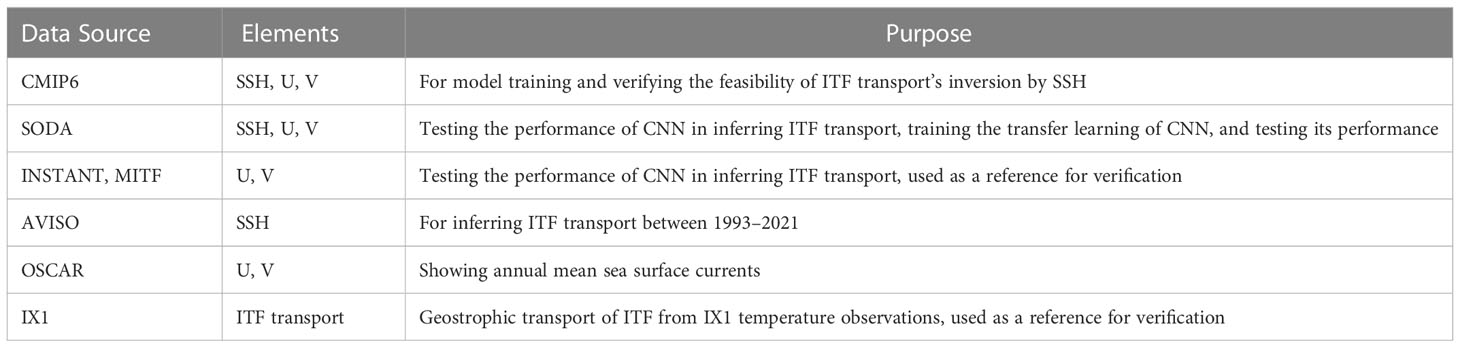
Table 1 The specifics of the data used for this study.

TABLE 2

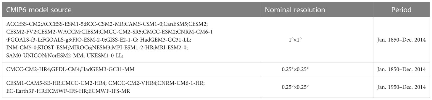
Table 2 Details of the CMIP6 models used in this study.

The data for transfer learning and testing are a reanalysis dataset from the University of Maryland’s Simple Ocean Data Assimilation (SODA 2.2.4; details in Table 1). The SODA dataset assimilates ocean station data, mooring temperature and salinity time series, various types of surface temperature and salinity observations, and nighttime infrared satellite SST data. The physical output quantity is mapped to a uniform 0.5°×0.5°×40 grid in the form of a monthly average.

The observational data for comparison and verification of the model results come from the INSTANT program, the MITF program, Ocean Surface Current Analysis Real-time (OSCAR, Lagerloef et al., 2002), and the Archiving, Validation, and Interpretation of Satellite Oceanographic data (AVISO; see details in Table 1). The INSTANT moorings were deployed simultaneously to measure the ITF from the Pacific inflow at Makassar Strait and Lifamatola Passage to the Indian Ocean export channels of Timor, Ombai, and Lombok, from 2004 to 2006 (Sprintall et al., 2004). The mooring array was designed to measure the ITF’s velocity, temperature, and salinity profiles. In this study, we used the sum of volume transports at three outflow straits, i.e., the Lombok strait, the Timor Passage, and the Ombai Strait, as the ITF transport.

The MITF moorings were deployed simultaneously to measure the ITF from the Pacific inflow at Makassar Strait; the mooring data in the Makassar Strait spans more than 13 years (Susanto et al., 2012; Gordon et al., 2019). The XBT survey along the IX1 section between Fremantle, Western Australia and the Sunda Strait, Indonesia has been operating for more than 30 years. The time series of geostrophic transport of ITF can be obtained through the IX1 temperature data (Liu et al., 2015). The OSCAR is an experimental processing system and data center that provides surface velocity fields in the tropical Pacific Ocean. Surface currents from the OSCAR were calculated from satellite altimeters and vector wind data using methods developed during the TOPEX/Poseidon altimeter research mission (Bonjean and Lagerloef, 2002). The sea surface height data are a multisource altimeter sea surface height fusion product provided by AVISO, with a spatial resolution of 0.25°×0.25° and a temporal resolution of 1 month. The data were primarily fused with satellite data from several altimeters, including TOPEX/POSEIDON, Jason. 1, and ERS/Envisat (AVISO, 2020).

To facilitate deep learning, the SSH data from SODA and CMIP6 were linearly interpolated. Given that the ITF is controlled by a large-scale gradient over the Indo-Pacific Ocean, we used SSH from a broad region 30°E–286°E and 44°S–44°N (Figure 1). In SODA and CMIP6 models, ITF transport was defined as the volume of transport across the section at 113.5°E (8.5°S–22.5°S). The CMIP6 data was divided into three sets: train set, verification set, and test set. Figure 2 presents a schematic diagram of the training and operation of the CNN model with the above datasets.

FIGURE 1

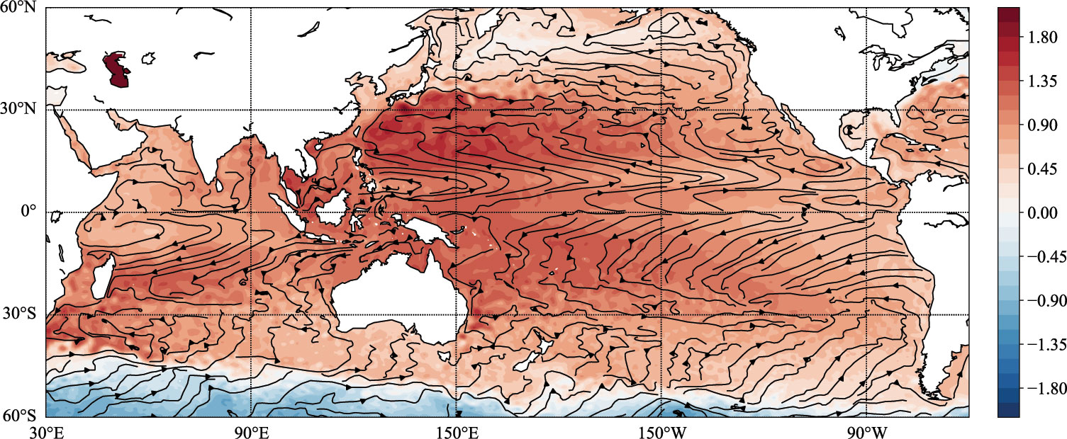
Figure 1 Annual mean sea surface currents (vectors, OSCAR) and sea surface height (color, AVISO) in 2018.

FIGURE 2

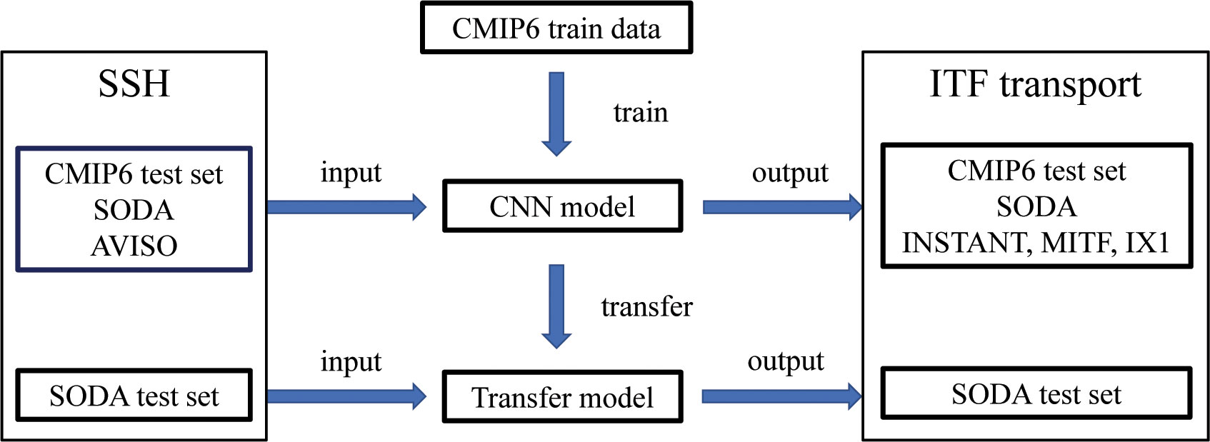
Figure 2 A schematic diagram displaying the training and operation of a CNN model with various datasets.

The train set contains model data from 1850 to 1974, the verification set contains data from 1974 to 1994, and the test set contains data from 1994 to 2014. SODA data from 1871 to 1974 was used for transfer learning, while SODA data from 1980 to 2010 was used for testing. ITF transport was standardized before being incorporated into the deep-learning model.

The standardized z-score method is based on the following equation:

$\begin{array}{ll}\text{Z}=\frac{X-\mu }{\sigma },& (1)\end{array}$

where μ is the mean value of the train data, σ is the standard deviation of the train data, X is the transport of ITF, and Z is the standardized ITF transport. The z-score method can be applied to numerical data and is not affected by the magnitude of the data, because its function is to eliminate the inconvenience caused by the magnitude of the analysis.

2.2 Methods

Figure 3 shows the CNN architecture used in this study, which consists of four convolutional layers and four pooling layers. The variables of the input layer correspond to the SSH from time t−2 months to time t (in months), between 30°E–286°E and 44°S–44°N. Each convolution layer was convoluted by a 4×4 convolutional filter. To filter the output of previous layers, a predefined non-linear activation function and batch normalization were applied. After the four convolutions, the features are flattened into one-dimensional vectors and transferred to a two-layer fully connected neural network to predict ITF transport. ReLU (Pedamonti, 2018) was used as a non-linear activation function. The role of the activation function is to add non-linear properties to the network, allowing it to learn highly complex mappings.

FIGURE 3

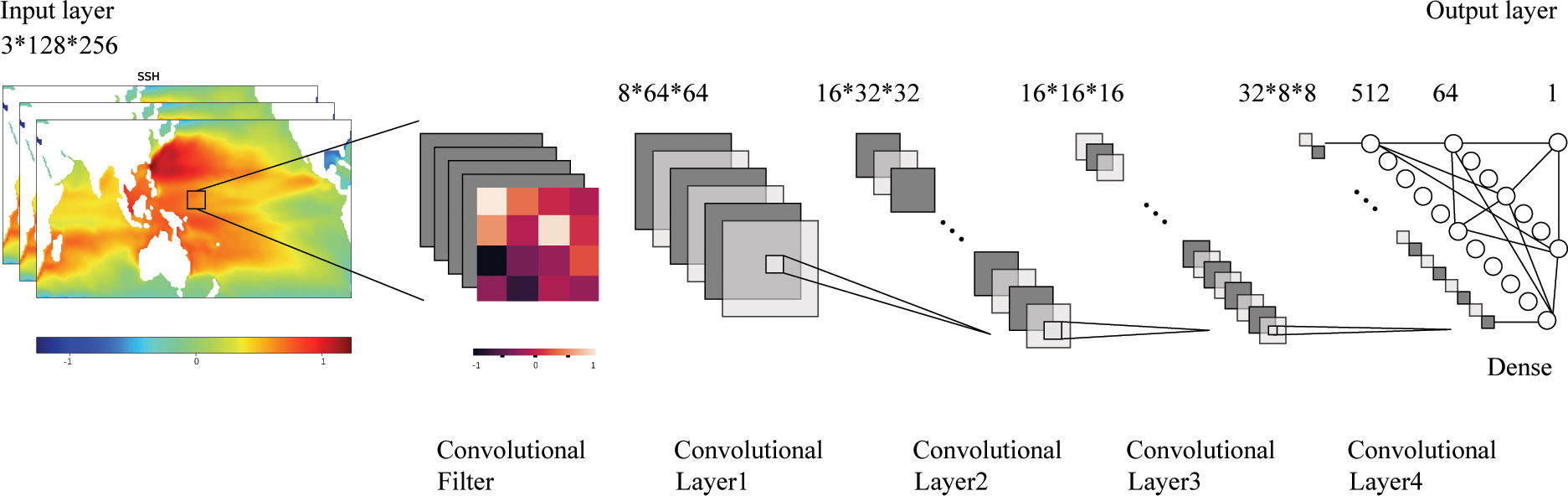
Figure 3 CNN Architecture diagram.

The convolution layer works by convolving a small convolution filter (Figure 3) onto the input image and then passing each output pixel through the activation function, mapping the input (SSH image) to the output (ITF transport). The CNN’s convolutional filtering matrices are not present, but the gradient descent algorithm is used to optimize input and output data until they reach the minimum value of the target error function (Kingma and Ba, 2014).

The horizontal dimension of the pooling kernel is 4×4. The pooling kernel continuously reduces the previous layer’s data by selecting the most significant pixel among the locally selected pixels. The cost of transport prediction error is calculated by taking the derivative of the network’s weight value. The weight value of the convolution filter and the entire connection is then trained using backpropagation to update each weight value to reduce the loss. The power of CNN lies in the fact that the filters of each convolutional layer are learned from data as part of the training process rather than being prespecified.

Deep learning necessitates the selection of hyperparameters to optimize the network, specifically: the horizontal dimension of the convolution matrix is 4×4, the Adam Optimiser algorithm (Kingma and Ba, 2014) is used to achieve gradient descent, and the default learning rate is set to 0.001. The dropout probability is set to 30% to reduce overfit and is implemented between the first and second fully connected layers. The neural network loss function is defined as the mean square error between the actual transport of ITF and the predicted transport by CNN. The network is coded in Python and employs Google’s machine-learning package TensorFlow (Abadi et al., 2016).

Insufficient training data causes overfitting or skill reduction in any neural network. High-complexity networks with more trainable parameters typically achieve better prediction skills, but they require more training data (George et al., 2021). The number of free parameters in the CNN in this paper was O(10⁶), and this was updated iteratively using the random gradient descent method and training data with a number of O(10⁴). Regularization techniques are used in CNN optimization to detect and prevent overfitting. This method divides data into independent train sets, verification sets, test sets, and random dropout of neurons.

We also compared results from various methods, including: (1) support vector machines (SVM); (2) logistic regression with the penalty term set to L2 and the regularization coefficient set to 1; (3) random forest, in which we implemented a random forest with 1,000 tree estimators; (4) deep fully connected neural networks (DNN), in which we used four layers of neural networks with 8,000, 1,250, 256, and 64 neurons, ReLU activation function, mean square error as the loss function, and no dropout; (5) a residual network (ResNet) with over 17 million parameters; and a (6) convolutional LSTM network with two convolutional LSTM layers, one convolutional layer, and two fully connected layers. All of the methods described above used the same dataset.

To evaluate the performance of CNN and other data-driven methods, skill S and correlation coefficient R were defined as:

$\begin{array}{ll}\begin{array}{c}S=1-{\left(\frac{\frac{1}{N}{\sum }_{i=1}^N{(y_{p,i}-y_{t,i})}^2}{{\sigma }_{y_t}^2}\right)}^{\frac{1}{2}}\\ R=\frac{\frac{1}{N}{\sum }_{i=1}^N\left(y_{p,i}-{\overline{y}}_p\right)\left(y_{t,i}-{\overline{y}}_t\right)}{{\sigma }_{y_p}{\sigma }_{y_t}},\end{array}& (2)\end{array}$

where y_p and  y_t are the predicted transport and the actual transport and σ_yp and σ_yt are the standard deviations of the actual and predicted transport of ITF.

The skill and correlation coefficient of perfect prediction is approaching. However, there are significant differences between these two indicators. Skill S is the monotone decreasing function of mean square error, which is negative when the prediction is worse than the data average (George et al., 2021). Anyway, it is not sensitive to measurement accuracy in some cases and often needs to be multiplied by a constant.

3 Results

The ITF transport of verification and test data was built using CNN training of CMIP6 data. CNN’s epoch was set to 100. One epoch indicates that all data have been sent to the network, completing the forward computation and backpropagation process. Figure 4 demonstrates that the predictive skill of verification data reached a high level around epoch 30. The average S showed a peak of 0.69 (Figure 4), corresponding to a high correlation coefficient of 0.95 that was significant at a 99% confidence level between deep-learning transport and actual transport of CMIP6. This suggests that the CNN was very efficient at extracting the required information from the SSH to infer the ITF transport of CMIP6. Training for too many epochs does not result in better verification and test data results. The training skill was expected to improve further with the development of the CNN model. Nonetheless, the skill of verification and test data was approximately 0.69. The skill stabilized in a short epoch, indicating that excessive training may lead to overfitting.

FIGURE 4

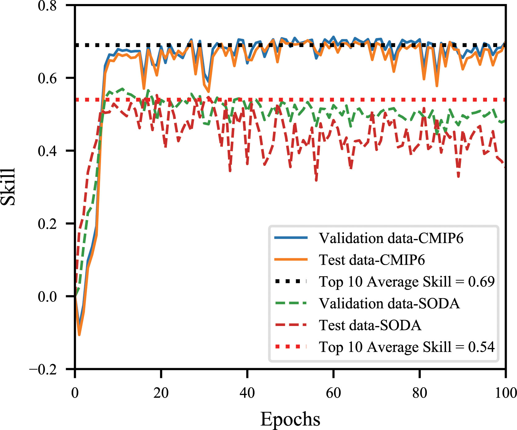
Figure 4 Evolution of skills with deep learning. The solid lines represent deep-learning skills with CMIP6, whereas the dotted lines (except black) represent SODA skills. The solid blue line represents the verification data, the orange line the test data, and the black dotted line represents the average of the top 10 skills using CMIP6. The green dotted line represents verification data, the red dotted line represents test data, and the pink dotted line denotes the average of the top 10 skills with SODA.

Figures 5A, B show the distribution of inferred and actual ITF of CMIP6 qualitatively and quantitatively, and the inferred ITF corresponded well with the actual ITF. A comparison of CNN-inferred and actual ITF transports of CMIP6 revealed that the CNN is capable of producing a reasonable ITF transport time series (Figure 5C). Despite the fact that the CNN explained up to 90% of ITF transport variation (Figure 5A), it appeared that the results inferred by CNN had a systematic bias, which may be a result of the limitations of using only SSH data. The CNN consistently underestimated the peak values of ITF transportation (Figures 5B, C). Even when increasing the number of extreme ITF transport training examples, testing various optimizers (e.g., stochastic gradient descent [SGD], Adam), loss functions (mean absolute error and mean square error), and weight regularization (L1, L2), this underestimation is unavoidable.

FIGURE 5

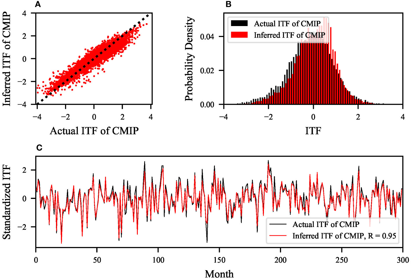
Figure 5 A comparison of CNN-inferred and actual ITF CMIP6 transports. (A) The x-axis represents the range of CMIP6 actual ITF, while the y-axis represents the inferred ITF for each actual ITF. The black dotted lines show where the inferred ITF equals the CMIP6-actual ITF. The scatter diagram shows that the CNN explains more than 90% of the traffic variance (max achieves R² = 0.90). (B) The histogram demonstrates the bias of underestimated transportation extremes. The actual ITF transport is shown in black, while the inferred ITF transport is shown in red. (C) Time series of actual transport (black) and inferred ITF transport (red) when the skill is 0.69.

The CNN showed excellent performance in inferring the ITF transport and we then directly substituted the data from SODA and AVISO into the model trained by the CMIP 6 (ITF without transfer, i.e., all the samples for training, test, and prediction were from CMIP 6 simulations). The average test skill of SODA data acquired by the CNN peaked at 0.54 (Figure 4). Owing to overfitting, the skill dropped rapidly after the training epoch reaches approximately 70, so the training step size should be set between 30 and 70. When compared with the CNN model based on CMIP6, SODA’s test skills were significantly lower, and its inferring ability is less stable.

To compensate for the small sample size of the reanalysis data, we conducted transfer learning on SODA using the training model with CMIP6 data. The R of inferred SODA ITF transport with transfer learning was 0.91, while the R of inferred SODA ITF transport without transfer learning was 0.86. The correlation of inferring with transfer learning was slightly improved when compared to the model without transfer learning (Figure 6). In inferring extreme transport, transfer learning was slightly inferior to that without transfer learning, but the degree of fitting was better than the model without transfer learning (Figure 6).

FIGURE 6

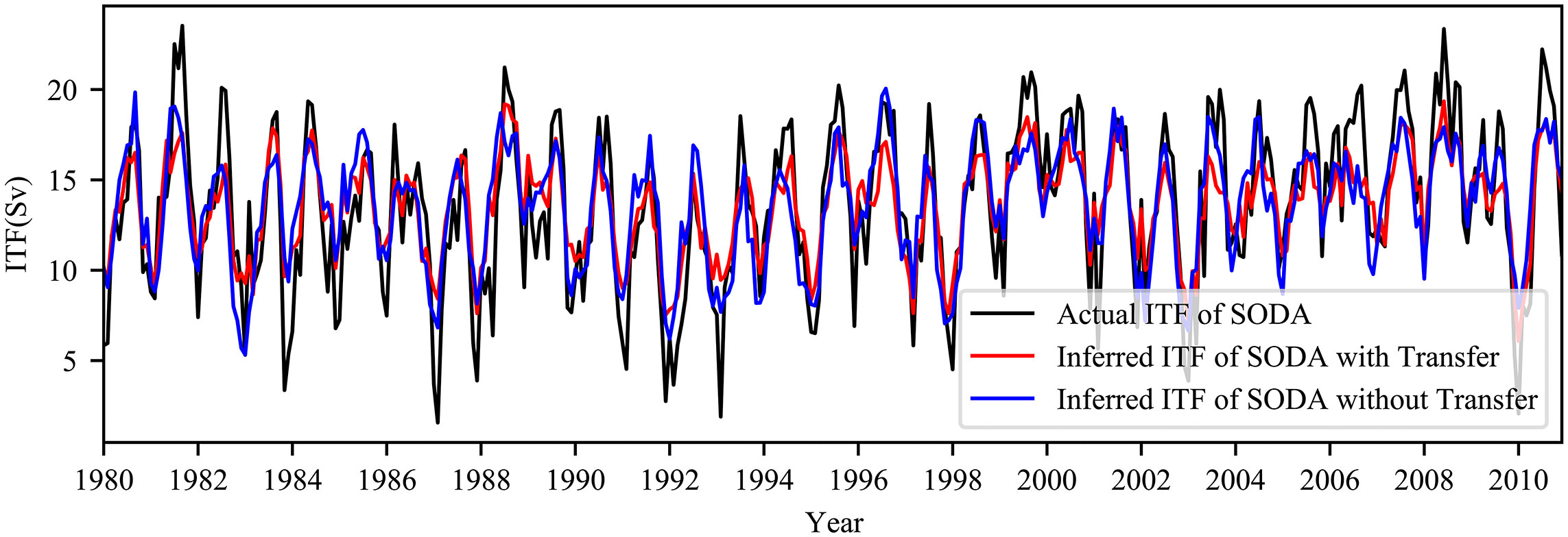
Figure 6 Comparison between CNN-inferred SODA with transfer (red), CNN-inferred SODA without transfer (blue), and actual ITF transports of SODA (black).

Figure 7 shows a comparison of various statistical methods. We found that the CNN explains more than 90% of the variance and shows a better performance than other statistical methods (logistic regression, random forest, SVM, or DNN), as expected (Figure 7). We also put different CNN variants to the test, such as the ResNet and convolutional LSTM. It is interesting to note that ResNet performed similarly to the CNN, despite having more parameters (Figure 7). The addition of recurrent neural networks did not improve the CNN’s capability. Given that the CNN has an excellent ability to infer ITF transport with the SSH, we used the same model to further investigate the deep-learning approach of predicting long-term ITF transport with the CNN. It should be noted that these various statistical methods contain very different parameters that may potentially influence the comparison.

FIGURE 7

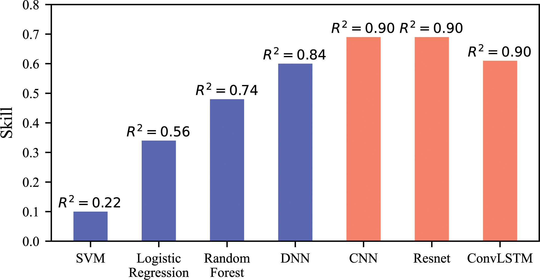
Figure 7 A comparison of various statistical methods for inferring with CMIP6. The y-axis represents the inference abilities of various technologies, such as SVM, logistic regression, random forest, DNN, CNN, ResNet, and convolutional LSTM network. The R² of each column represents the proportion of inferred variance.

We then generated an updated long-term and continuous time series of ITF transport using the CNN-based deep-learning approach and updated satellite observations of SSH (Figure 8). The CNN model’s inference of ITF transport was validated by comparing it with observations (Figure 8). It appeared that the ITF from deep learning captures the general variability of ITF: the correlation coefficient was 0.43 between IX1-observed ITF and 13-month-running-mean time series of CNN-inferred ITF with satellite observation, 0.57 between INSTANT-observed ITF and CNN-inferred ITF with satellite observations, and 0.52 between MITF-observed ITF and CNN-predicted ITF with satellite observations, all of which were significant at the 99% confidence level (Figure 8). The deep-learning ITF differed from the observations primarily in terms of peaks and valleys, which may be associated with the ability of CMIP6 models to reproduce the ITF’s extremes (figure not shown).

FIGURE 8

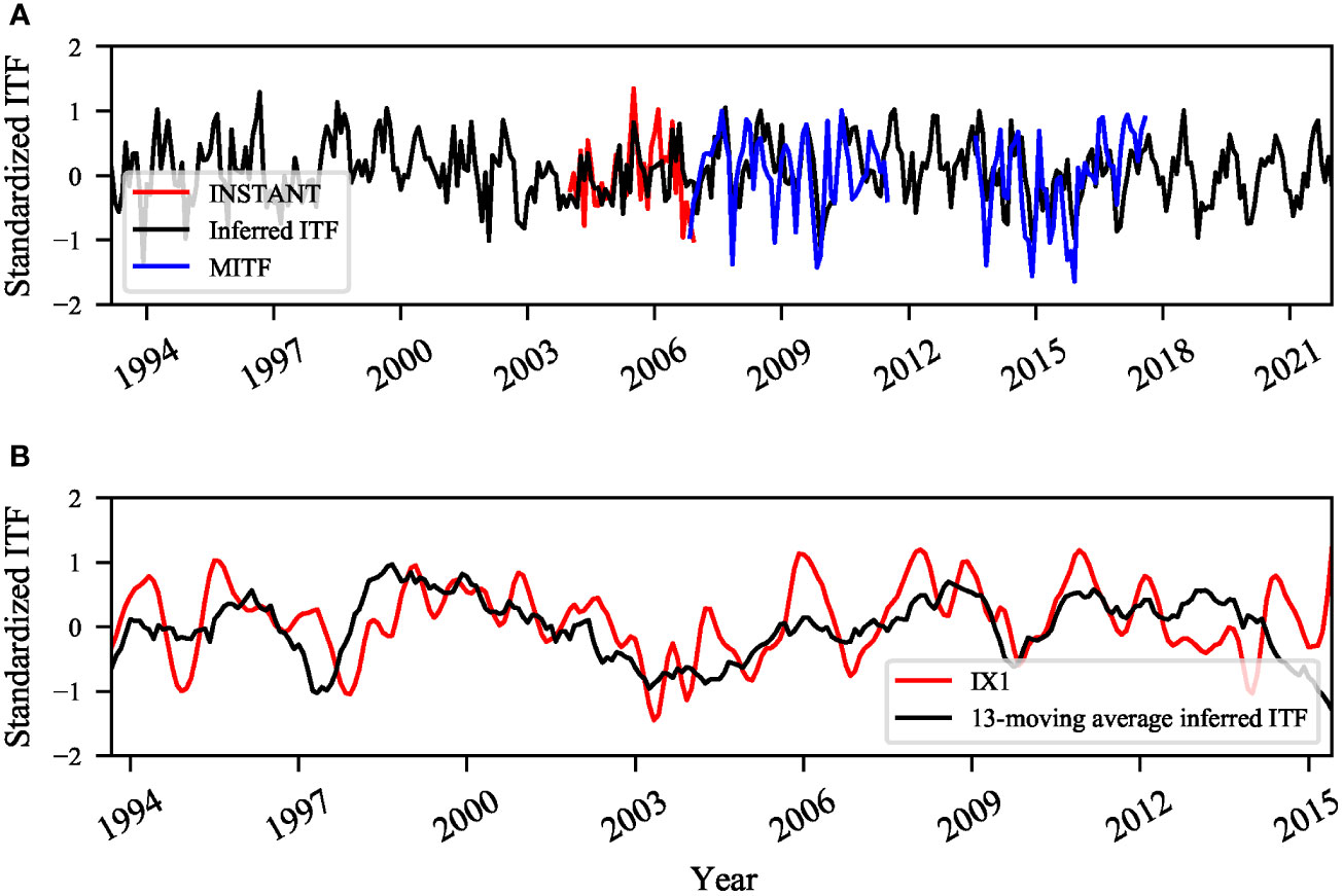
Figure 8 Comparison between CNN-inferred and actual ITF transports of observations. (A) inferred-predicted (black), ITF transports from INSTANT observation (red), and MITF (blue). (B) Thirteen-month-running-mean CNN-inferred (black) and actual ITF transports of IX1 (red).

Figure 9 compares the predicted ITF transport of SODA with the actual ITF after transfer learning with different time leads. As shown in Figure 9, the R decreased overall as the time lead increased, and the CNN model could make a valid prediction (R>0.5) with a lead time of up to approximately 7 months. It should be noted that a 12-month moving average is used before calculating the correlation coefficient between the actual ITF and predicted ITF transports to reduce the influence of the ITF’s strong seasonality, and it shows that including of seasonality leads to a higher correlation coefficient between the actual ITF and predicted ITF transports. Figure 10 compares the predicted ITF transport from various models with the actual ITF transport (time series are 12-month smoothed to focus on interannual variability). The CNN was more effective and produced a longer forecast than other models (Figures 9 and 10).

FIGURE 9

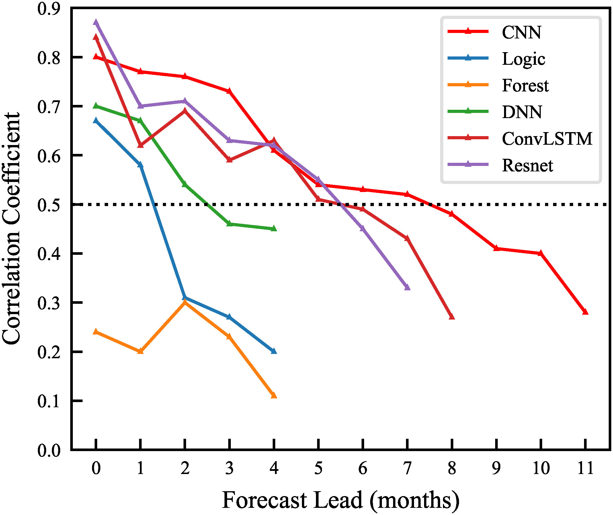
Figure 9 Comparison of actual ITF and predicted ITF transport of SODA using various models.

FIGURE 10

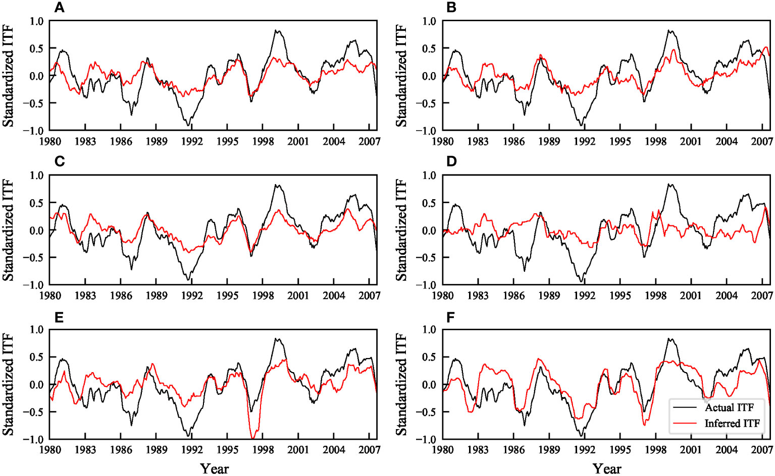
Figure 10 Comparison between actual ITF and inferred ITF transport of SODA with different models. (A) CNN. (B) Resnet. (C) Convolutional LSTM. (D) Forest. (E) Logic. (F) DNN.

4 Discussion and conclusion

In this study, we investigated the deep-learning approach for inferring and predicting ITF transport with SSH images using model simulations from CMIP6 and reanalysis data products. We discovered that the CNN-based deep-learning approach with SSH images can generate a reasonable time series of ITF transport that captures approximately 90% of the actual ITF variance. CNN-based deep learning with reanalysis data sets performed similarly well, reproducing approximately 80% of the variance of actual ITF transport. These findings imply that the CNN, which explicitly relies on two-dimensional pattern analysis, outperforms other traditional data-driven technologies, such as logistic regression (R² =0.56), random forest (R² =0.74), statistical vector machines (R² =0.22), and primary fully connected neural networks (R² =0.84).

Although the CNN performed admirably in predicting ITF transport, it appears that the CNN’s prediction has a systematic bias, and the peak values of ITF transport were consistently underestimated by the CNN. Even when some methods, such as increasing the number of extreme ITF transport training examples, testing various optimizers, loss functions, and weight regularization, were used, bias and underestimation remained unavoidable. The bias and underestimation indicate that the skill limitations are due to the inherent incompleteness of the information in SSH, rather than a lack of training data or weaknesses in the CNN architecture.

It is well known that the network parameters most likely influence deep-learning performance. Different network parameters were also tested in this study. We employed various sizes of convolutional filters (3×3, 4×4, 5×5, and 7×7) and pooling filters (2×2 and 4×4). Larger convolutional filters produced worse predictions than smaller convolutional filters. We discovered that a 3×3 convolutional filter predicts similarly to a 4×4 convolutional filter, but a larger convolutional filter means fewer parameters. Additionally, we tested various optimizers (SGD and Adam), loss functions (mean absolute error and mean square error), and weight regularization (L1 and L2), and the CNN was found to be the most efficient choice. We attempted to improve the performance of the CNN by increasing the number of parameters and the cyclic neural network, which can improve the performance at month 0. However, as prediction time increased, the prediction ability of the two remained inferior to that of the CNN. This means that in some cases, more complex networks do not produce better results. We also tried increasing the size of the input from t−9 months to time t (in months), and the performance of ResNet and convolutional LSTM improved slightly.

The performance of the CNN in the model and reanalysis data demonstrates that there is enough information in SSH to predict ITF transport. However, further improvement in predicting ITF transport using a deep-learning approach is required and is dependent on at least two factors. On the one hand, the amount of training data required for the CNN supervised learning is quite large, necessitating a sampling size of O(10⁴). As a result, advanced deep-learning techniques that reduce the amount of essential training data by at least one order of magnitude are required, as is the ability to forecast in the long term. On the other hand, considering that the ITF is influenced by baroclinic processes as well, the subsurface information is also important for inferring and predicting ITF transport. As a result, a better deep-learning approach should use subsurface information in training the model, even though observing the subsurface ocean is obviously very different from satellite-based sea surface observation. Furthermore, as the large-scale pressure gradient between the Pacific Ocean and the Indian Ocean is the driver of ITF and some key regions seem to determine the ITF (e.g., Susanto et al., 2007; Tillinger and Gordon, 2009), the deep-learning approach might be further improved if we additionally consider the SSH in these key regions. All of this points to a bright future for monitoring and predicting important large-scale ocean circulations, such as the ITF.

Data availability statement

The original contributions presented in the study are included in the article/supplementary material. Further inquiries can be directed to the corresponding author.

Author contributions

SH designed the study. LX and SH conducted the analysis and wrote the initial draft of the paper. All authors contributed to the article and approved the submitted version.

Funding

This study is supported by the Shandong Provincial Natural Science Foundation (ZR2020JQ18), the Strategic Priority Research Program of the Chinese Academy of Sciences (CAS) (XDB42010403), the National Natural Science Foundation of China (42022040), and the Laoshan Laboratory (2022LSL010304). S. Hu is a member of the CAS Interdisciplinary Innovation Team (JCTD-2020-12) and the Youth Innovation Promotion Association of CAS. We are grateful to Qin- Yan Liu for providing the time series of ITF transport based on IX1 observations and to Mingting Li for helping us access the MITF time series.

Acknowledgments

The altimeter data were produced by SSALTO/Duacs and available at https://sso.altimetry.fr/(readers may need to register for an account with AVISO to access the data). The CMIP6 simulations can be accessed at https://esgf-node.llnl.gov/search/cmip6/. The International Nusantara Stratification and Transport (INSTANT) data can be accessed at http://www.marine.csiro.au/~cow074/instantdata.htm. The SODA 2.2.4 and OSCAR datasets were obtained from the Asia-Pacific Data Research Center of the International Pacific Research Center at the University of Hawaiʻi at Mānoa (http://apdrc.soest.hawaii.edu/index.php).

Conflict of interest

The authors declare that the research was conducted in the absence of any commercial or financial relationships that could be construed as a potential conflict of interest.

Publisher’s note

All claims expressed in this article are solely those of the authors and do not necessarily represent those of their affiliated organizations, or those of the publisher, the editors and the reviewers. Any product that may be evaluated in this article, or claim that may be made by its manufacturer, is not guaranteed or endorsed by the publisher.

References

Abadi M., Agarwal A., Barham P., Brevdo E., Chen Z., Citro C., et al. (2016). Tensorflow: Large-scale machine learning on heterogeneous distributed systems. arXiv preprint arXiv 1603, 4467. doi: 10.48550/arXiv.1603.04467

CrossRef Full Text | Google Scholar

Anderson G. J., Lucas D. D. (2018). Machine learning predictions of a multiresolution climate model ensemble. Geophysical Res. Letters 45 (9), 4273–4280. doi: 10.1029/2018GL077049

CrossRef Full Text | Google Scholar

AVISO (2020) Satellite altimetry data. Available at: https://www.aviso.altimetry.fr/en/home.html.

Google Scholar

Bolton T., Zanna L. (2019). Applications of deep learning to ocean data inference and subgrid parameterization. J. Adv. Modeling Earth Systems 11 (1), 376–399. doi: 10.1029/2018MS001472

CrossRef Full Text | Google Scholar

Bonjean F., Lagerloef G. S. (2002). Diagnostic model and analysis of the surface currents in the tropical pacific ocean. J. Phys. Oceanography 32 (10), 2938–2954. doi: 10.1175/1520-0485(2002)032<2938:DMAAOT>2.0.CO;2

CrossRef Full Text | Google Scholar

Cybenko G. (1989). Approximation by superpositions of a sigmoidal function. Mathematics Control Signals Systems 2 (4), 303–314. doi: 10.1007/BF02551274

CrossRef Full Text | Google Scholar

Esteves J. T., de Souza Rolim G., Ferraudo A. S. (2019). Rainfall prediction methodology with binary multilayer perceptron neural networks. Climate Dynamics 52 (3), 2319–2331. doi: 10.1007/s00382-018-4252-x

CrossRef Full Text | Google Scholar

Feng M., Benthuysen J., Zhang N., Slawinski D. (2015). Freshening anomalies in the Indonesian throughflow and impacts on the leeuwin current during 2010–2011. Geophysical Res. Letters 42 (20), 8555–8562. doi: 10.1002/2015GL065848

CrossRef Full Text | Google Scholar

Feng M., Zhang N., Liu Q., Wijffels S. (2018). The Indonesian throughflow, its variability and centennial change. Geosci. Letters 5 (1), 1–10. doi: 10.1186/s40562-018-0102-2

CrossRef Full Text | Google Scholar

George T. M., Manucharyan G. E., Thompson A. F. (2021). Deep learning to infer eddy heat fluxes from sea surface height patterns of mesoscale turbulence. Nat. Commun. 12 (1), 1–11. doi: 10.1038/s41467-020-20779-9

PubMed Abstract | CrossRef Full Text | Google Scholar

Gordon A. L. (1986). Interocean exchange of thermocline water. J. Geophysical Research: Oceans 91 (C4), 5037–5046. doi: 10.1029/JC091iC04p05037

CrossRef Full Text | Google Scholar

Gordon A. L. (2005). Oceanography of the Indonesian seas and their throughflow. Oceanography 18 (4), 14–27. doi: 10.5670/oceanog.2005.01

CrossRef Full Text | Google Scholar

Gordon A. L., Napitu A., Huber B. A., Gruenburg L. K., Pujiana K., Agustiadi T., et al. (2019). Makassar strait throughflow seasonal and interannual variability: An overview. J. Geophysical Research: Oceans 124 (6), 3724–3736. doi: 10.1029/2018JC014502

CrossRef Full Text | Google Scholar

Gordon A. L., Sprintall J., Van Aken H. M., Susanto D., Wijffels S., Molcard R., et al. (2010). The Indonesian throughflow during 2004–2006 as observed by the INSTANT program. Dynamics Atmospheres Oceans 50 (2), 115–128. doi: 10.1016/j.dynatmoce.2009.12.002

CrossRef Full Text | Google Scholar

Gordon A. L., Susanto R. D., Ffield A. (1999). Throughflow within makassar strait. Geophysical Res. Letters 26 (21), 3325–3328. doi: 10.1029/1999GL002340

CrossRef Full Text | Google Scholar

Ham Y. G., Kim J. H., Luo J. J. (2019). Deep learning for multi-year ENSO forecasts. Nature 573 (7775), 568–572. doi: 10.1038/s41586-019-1559-7

PubMed Abstract | CrossRef Full Text | Google Scholar

Hornik K. (1991). Approximation capabilities of multilayer feedforward networks. Neural Networks 4 (2), 251–257. doi: 10.1016/0893-6080(91)90009-T

CrossRef Full Text | Google Scholar

Hu S., Lu X., Li S., Wang F., Guan C., Hu D., et al. (2021). Multi-decadal trends in the tropical pacific western boundary currents retrieved from historical hydrological observations. Sci. China Earth Sci. 64 (4), 600–610. doi: 10.1360/SSTe-2020-0148

CrossRef Full Text | Google Scholar

Hu S., Sprintall J. (2016). Interannual variability of the Indonesian throughflow: the salinity effect. J. Geophysical Research: Oceans 121, 2596–2615. doi: 10.1002/2015JC011495

CrossRef Full Text | Google Scholar

Hu S., Sprintall J. (2017). Observed strengthening of interbasin exchange via the Indonesian seas due to rainfall intensification. Geophysical Res. Letters 44 (3), 1448–1456. doi: 10.1002/2016GL072494

CrossRef Full Text | Google Scholar

Hu S., Sprintall J., Guan C., McPhaden M. J., Wang F., Hu D., et al. (2020). Deep-reaching acceleration of global mean ocean circulation over the past two decades. Sci. Advances 6 (6), eaax7727. doi: 10.1126/sciadv.aax7727

CrossRef Full Text | Google Scholar

Hu D., Wang F., Wu L., Chen D., Liu Q., Tian J., et al. (2011). Northwestern pacific ocean circulation and climate experiment (NPOCE) Science/Implementation plan (China Ocean Press: China), 100.

Google Scholar

Hu D., Wu L., Cai W., Gupta A. S., Ganachaud A., Qiu B., et al. (2015). Pacific western boundary currents and their roles in climate. Nature. 522, 299–308. doi: 10.1038/nature14504

PubMed Abstract | CrossRef Full Text | Google Scholar

Hu S., Zhang Y., Feng M., Du Y., Sprintall J., Wang F., et al. (2019). Interannual to decadal variability of upper-ocean salinity in the southern Indian ocean and the role of the Indonesian throughflow. J. Climate 32 (19), 6403–6421. doi: 10.1175/JCLI-D-19-0056.1

CrossRef Full Text | Google Scholar

Kingma D. P., Ba J. (2014). Adam: A method for stochastic optimization. arXiv preprint arXiv 1412, 6980. doi: 10.48550/arXiv.1412.6980

CrossRef Full Text | Google Scholar

Lagerloef G. S., Mitchum G. T., Bonjean F., Cheney R. (2002). Oscar (ocean surface currents analysis - real time): An operational resource for various maritime applications and el nio monitoring in the tropical pacific using jason1 data. Fall Meeting San Francisco, CA, Amer. Geophys. Union, Abstract OS51C-12.

Google Scholar

Lee S. K., Park W., Baringer M. O., Gordon A. L., Huber B., Liu Y. (2015). Pacific origin of the abrupt increase in Indian ocean heat content during the warming hiatus. Nat. Geoscience. 8 (6), 445–449. doi: 10.1038/NGEO2438

CrossRef Full Text | Google Scholar

Li M., Gordon A. L., Wei J., Gruenburg L. K., Jiang G. (2018). Multi-decadal timeseries of the Indonesian throughflow. Dynamics Atmospheres Oceans 81, 84–95. doi: 10.1016/j.dynatmoce.2018.02.001

CrossRef Full Text | Google Scholar

Liu Q. Y., Feng M., Wang D., Wijffels S. (2015). Interannual variability of the Indonesian throughflow transport: A revisit based on 30 year expendable bathythermograph data. J. Geophysical Research: Oceans 120 (12), 8270–8282. doi: 10.1002/2015JC011351

CrossRef Full Text | Google Scholar

Liu W., Xie S. P., Lu J. (2016). Tracking ocean heat uptake during the surface warming hiatus. Nat. Commun. 7 (1), 1–9. doi: 10.1038/ncomms10926

CrossRef Full Text | Google Scholar

Ma J., Feng M., Lan J., Hu D. (2020). Projected future changes of meridional heat transport and heat balance of the Indian ocean. Geophysical Res. Letters. 47 (4), e2019GL086803. doi: 10.1029/2019GL086803

CrossRef Full Text | Google Scholar

Meyers G., Bailey R. J., Worby A. P. (1995). Geostrophic transport of Indonesian throughflow. Deep Sea Res. Part I: Oceanographic Res. Papers 42 (7), 1163–1174. doi: 10.1016/0967-0637(95)00037-7

CrossRef Full Text | Google Scholar

Pedamonti D. (2018). Comparison of non-linear activation functions for deep neural networks on MNIST classification task. arXiv preprint. arXiv 1804, 2763. doi: 10.48550/arXiv.1804.02763

CrossRef Full Text | Google Scholar

Phillips H. E., Tandon A., Furue R., Hood R., Ummenhofer C. C., Benthuysen J. A., et al. (2021). Progress in understanding of Indian ocean circulation, variability, air–sea exchange, and impacts on biogeochemistry. Ocean Science 17 (6), 1677–1751. doi: 10.5194/os-17-1677-2021

CrossRef Full Text | Google Scholar

Santoso A., England M. H., Kajtar J. B., Cai W. (2022). Indonesian Throughflow variability and linkage to ENSO and IOD in an ensemble of CMIP5 models. J. Climate 35 (10), 3161–3178. doi: 10.1175/JCLI-D-21-0485.1

CrossRef Full Text | Google Scholar

Sen Gupta A., McGregor S., Van Sebille E., Ganachaud A., Brown J. N., Santoso A. (2016). Future changes to the Indonesian throughflow and pacific circulation: The differing role of wind and deep circulation changes. Geophysical Res. Letters 43 (4), 1669–1678. doi: 10.1002/2016GL067757

CrossRef Full Text | Google Scholar

Shilimkar V., Abe H., Roxy M. K., Tanimoto Y. (2022). Projected future changes in the contribution of indo-pacific sea surface height variability to the Indonesian throughflow. J. Oceanography 78 (5), 337–352. doi: 10.1007/s10872-022-00641-w

CrossRef Full Text | Google Scholar

Shinoda T., Han W., Metzger E. J., Hurlburt H. E. (2012). Seasonal variation of the Indonesian throughflow in makassar strait. J. Phys. Oceanography 42 (7), 1099–1123. doi: 10.1175/JPO-D-11-0120.1

CrossRef Full Text | Google Scholar

Sprintall J., Gordon A. L., Koch-Larrouy A., Lee T., Potemra J. T., Pujiana K., et al. (2014). The Indonesian seas and their role in the coupled ocean–climate system. Nat. Geoscience. 7 (7), 487–492. doi: 10.1038/ngeo2188

CrossRef Full Text | Google Scholar

Sprintall J., Gordon A. L., Wijffels S. E., Feng M., Hu S., Koch-Larrouy A., et al. (2019). Detecting change in the Indonesian seas. Front. Mar. Sci. 6. doi: 10.3389/fmars.2019.00257

CrossRef Full Text | Google Scholar

Sprintall J., Révelard A. (2014). The Indonesian throughflow response to indo-pacific climate variability. J. Geophysical Research: Oceans 119 (2), 1161–1175. doi: 10.1002/2013JC009533

CrossRef Full Text | Google Scholar

Sprintall J., Wijffels S., Gordon A. L., Ffield A., Molcard R., Susanto R. D., et al. (2004). INSTANT: A new international array to measure the Indonesian throughflow. Eos Trans. Am. Geophysical Union 85 (39), 369–376. doi: 10.1029/2004eo390002

CrossRef Full Text | Google Scholar

Sprintall J., Wijffels S. E., Molcard R., Jaya I. (2009). Direct estimates of the Indonesian throughflow entering the Indian ocean: 2004–2006. J. Geophysical Research: Oceans 114 (C7), C07001. doi: 10.1029/2008jc005257

CrossRef Full Text | Google Scholar

Sun S., Thompson A. F. (2020). Centennial changes in the Indonesian throughflow connected to the Atlantic meridional overturning circulation: The ocean's transient conveyor belt. Geophysical Res. Letters 47 (21), e2020GL090615. doi: 10.1029/2020GL090615

CrossRef Full Text | Google Scholar

Susanto R. D., Ffield A., Gordon A. L., Adi T. R. (2012). Variability of Indonesian throughflow within makassar strait 2004–2009. J. Geophysical Research: Oceans 117 (C9), C09013. doi: 10.1029/2012JC008096

CrossRef Full Text | Google Scholar

Susanto R. D., Gordon A. L., Sprintall J. (2007). Observations and proxies of the surface layer throughflow in lombok strait. J. Geophysical Research: Oceans 112 (C3), C03S92. doi: 10.1029/2006JC003790

CrossRef Full Text | Google Scholar

Susanto R. D., Song Y. T. (2015). Indonesian Throughflow proxy from satellite altimeters and gravimeters. J. Geophysical Research: Oceans 120 (4), 2844–2855. doi: 10.1002/2014JC010382

CrossRef Full Text | Google Scholar

Tillinger D., Gordon A. L. (2009). Fifty years of the Indonesian throughflow. J. Climate 22 (23), 6342–6355. doi: 10.1175/2009JCLI2981.1

CrossRef Full Text | Google Scholar

van Aken H. M., Brodjonegoro I. S., Jaya I. (2009). The deep-water motion through the lifamatola passage and its contribution to the Indonesian throughflow. Deep Sea Res. Part I: Oceanographic Res. Papers 56 (8), 1203–1216. doi: 10.1016/j.dsr.2009.02.001

CrossRef Full Text | Google Scholar

Wei Z., Li S., Susanto R. D., Wang Y., Fan B., Xu T., et al. (2019). An overview of 10-year observation of the south China Sea branch of the pacific to Indian ocean throughflow at the karimata strait. Acta Oceanologica Sin. 38 (4), 1–11. doi: 10.1007/s13131-019-1410-x

CrossRef Full Text | Google Scholar

Wijffels S., Meyers G. (2004). An intersection of oceanic waveguides: Variability in the Indonesian throughflow region. J. Phys. Oceanography 34 (5), 1232–1253. doi: 10.1175/1520-0485(2004)034<1232:AIOOWV>2.0.CO;2

CrossRef Full Text | Google Scholar

Wyrtki K. (1961). Physical oceanography of the southeast Asian waters Vol. 2 (University of California: Scripps Institution of Oceanography).

Google Scholar

Wyrtki K. (1987). Indonesian Through flow and the associated pressure gradient. J. Geophysical Research: Oceans 92 (C12), 12941–12946. doi: 10.1029/JC092iC12p12941

CrossRef Full Text | Google Scholar

Xu G., Cheng C., Yang W., Xie W., Kong L., Hang R., et al. (2019). Oceanic eddy identification using an AI scheme. Remote Sensing. 11 (11), 1349. doi: 10.3390/rs11111349

CrossRef Full Text | Google Scholar

Xu T. F., Wei Z. X., Susanto R. D., Li S. J., Wang Y. G., Wang Y., et al. (2021). Observed water exchange between the south China Sea and Java Sea through karimata strait. J. Geophysical Research: Oceans. 126 (2), e2020JC016608. doi: 10.1029/2020JC016608

CrossRef Full Text | Google Scholar

Zeng X., Li Y., He R. (2015). Predictability of the loop current variation and eddy shedding process in the gulf of Mexico using an artificial neural network approach. J. Atmospheric Oceanic Technology 32 (5), 1098–1111. doi: 10.1175/JTECH-D-14-00176.1

CrossRef Full Text | Google Scholar