Biologically Important Areas II for cetaceans within U.S. and adjacent waters - Updates and the application of a new scoring system

1 Introduction

Anthropogenic activities in the marine environment continue to increase in number, geographic extent, and duration, resulting in increased potential risk to marine ecosystems worldwide (e.g., Poeta et al., 2017; de Vere et al., 2018; Gouveia et al., 2019; Duarte et al., 2021; O’Hara et al., 2021). Pursuant to multiple federal and state regulations, federal agencies, industry representatives, and members of the public conducting certain activities all share responsibility for assessing and minimizing the impacts of their activities on the environment and protected marine resources. For this specific U.S. effort, Biologically Important Areas (BIAs) represent areas and times in which cetaceans (whales, dolphins, or porpoises) are known to concentrate for activities related to reproduction, feeding, and migration, as well as ranges of small and resident populations. BIAs highlight important information, such as probable behavioral state, the presence of relatively sensitive life stages (e.g., calves), the existence of small populations with limited geographic ranges, and other information about what a species tends to do in a particular place and time. This information can help us better understand and predict how individual cetaceans are likely to respond to or be impacted by disturbances, how impacts may affect individual fitness, and where populations may be more susceptible to certain types of impacts. In the initial BIA effort (hereafter referred to as “BIA I”), Ferguson et al. (2015) described anthropogenic activities of concern for marine mammals, associated impacts, and how the spatiotemporal contextual information in BIAs is important in evaluating potential effects of those impacts on cetaceans.

Evidence continues to mount supporting the value of the information contained in BIAs for impact assessments for marine species (New et al., 2020; Pirotta et al., 2021). An understanding of where, when, how, and why marine mammals congregate and move is important when assessing direct interactions with human activities that can result in injurious or lethal impacts, such as vessel strike or fishing gear entanglement. Further, the growing body of evidence clearly indicates that an animal’s behaviors, activities, or states when exposed to the pervasive array of non-lethal stressors, such as underwater noise, can affect their immediate response (e.g., McHuron et al., 2018; Pirotta et al., 2021), with cumulative exposures potentially affecting individual fitness, which may ultimately result in population-level impacts (e.g., New et al., 2014; Dunlop et al., 2021; Pirotta et al., 2022).

To assess and predict the severity of marine mammal behavioral responses to underwater noise, Southall et al. (2021) emphasize the importance of subject-specific variables, such as behavioral state, whether calves are present, and other information highlighted by BIAs. In an extensive synthesis, they propose a new behavioral response severity scale for discrete exposures that rates response severity along three parallel and ethologically-based severity tracks: (1) survival (including effects on defense, resting, social interactions, and navigation); (2) reproduction (including mating and parenting behaviors); and, (3) foraging (encompassing search, pursuit, capture, and consumption). The severity rating indicates the likelihood that the response will result in a change in vital rates (e.g., through survival, energetic effects, or reproduction). Southall et al. (2021) strongly advocate for the robust and systematic reporting of key exposure metrics, including subject-specific metrics (e.g., behavioral state, whether calves are present), exposure context metrics (e.g., animal depth, proximity to the source of disturbance), and noise exposure metrics (e.g., exposure duration, maximum source level), in both experimental and observational studies, given the importance of these metrics in predicting responses. Further, they note that odontocetes with localized home ranges may experience long-term exposure to certain stressors, such as whale-watching, which cumulatively increase the likelihood of more severe effects, thus emphasizing the importance of identifying small and resident populations.

Another key tool in marine mammal risk assessment is the Population Consequences of Disturbance (PCoD) framework (National Resource Council, 2005; New et al., 2014), which conceptualizes how disturbance-induced changes in individual behavior and physiology affect populations through changes in individual health and vital rates. Keen et al. (2021) note that since the PCoD framework was first proposed, multiple models have been created to quantitatively evaluate the short- and long-term consequences of disturbance. PCoD models have been developed for several marine mammal species using a combination of matrix modeling, physiologically structured population modeling, bioenergetic modeling, and stochastic dynamic programming. These models have been parameterized via species-specific empirical data and alternative methods, including extrapolating from other species, proxy relations, and expert elicitation and informed assumptions when empirical data were lacking (Keen et al., 2021). Keen et al. (2021) synthesized the PCoD findings since 2005, reviewed common themes that have emerged, and highlighted essential intrinsic and extrinsic factors to consider when assessing risk to individuals and populations. One key factor is whether the disturbance source overlaps with biologically important habitats, such as those identified by BIAs. Citing multiple PCoD models, Keen et al. (2021) note that a population’s sensitivity to disturbance is strongly influenced by the importance of the disturbed area for foraging, reproduction, and migration.

BIAs that reflect the current ecological condition or status of a species provide critical information that is urgently needed for responsible management and conservation of cetaceans. In the eight years since the BIA I manuscripts were published, there have been changes in species distribution, density, abundance, and habitat use. The BIA II effort was designed to evaluate the latest information on cetacean ecology to ensure that the BIAs reflect the current and best available science.

The intended and appropriate use of BIAs cannot be overemphasized given the potential for mischaracterization and the confusion they could create. BIAs are compilations of the best available science and have no inherent or direct regulatory power. Neither the presence of, nor the associated scores for, a BIA should be interpreted as an indicator of vulnerability. BIAs may be used like any other scientific information (defined here to include data from formal scientific research, Indigenous knowledge, local knowledge, and community science) to support analyses and decisions, as appropriate, for the purposes of environmental planning, compliance, and protection. BIAs have been used by federal agencies and the public to support marine mammal impact assessments, and to inform the development of conservation, management, and mitigation measures for cetaceans, where appropriate, under existing authorities (e.g., the U.S. Marine Mammal Protection Act (MMPA), Endangered Species Act (ESA), National Environmental Policy Act (NEPA), and National Marine Sanctuaries Act (NMSA). However, BIAs have no legal, statutory, or regulatory power.

Of important note, because BIAs serve a different purpose and are defined differently, BIA delineation and scoring was conducted entirely independently of any consideration of critical habitat designations pursuant to the U.S. Endangered Species Act. Areas that NOAA has officially designated as critical habitat were only included as BIAs, either in part or whole, if they qualified as BIAs based on the definitions presented in this manuscript and the appropriate application of the scoring protocols. Critical habitat is defined in section 3 of the ESA as specific areas within the geographical area occupied by the species at the time of listing that contain physical or biological features essential to conservation of the species and that may require special management considerations or protection; and specific areas outside the geographical area occupied by the species if the agency determines that the area itself is essential for conservation of the species. Critical habitat is determined on the basis of the best available science, but the designation of critical habitat must also consider economic, national security, and other relevant impacts of specifying a particular area as critical habitat. BIAs are syntheses of science but do not need to meet this statutory definition and do not consider any of these other factors; therefore, not everything identified as critical habitat will meet the BIA criteria and vice versa.

BIAs were designed to address needs raised by managers who recognize the importance of the information ultimately included in BIAs to cetacean impact analyses. However, BIAs are but one tool available to inform marine mammal impact assessments and the development of protective measures. Any comprehensive impact assessment will need to consider information about the species and their habitat use, environmental pressures, and anthropogenic stressors. We stress the importance of other tools that are available to additionally support these efforts, including, but not limited to: ESA critical habitat, stock assessment reports, marine mammal abundance and density models (e.g., Roberts et al., 2016), unusual mortality event reports, PCoD models (Pirotta et al., 2021), climate vulnerability analyses (e.g., Lettrich et al., 2019), and ESA Recovery Plans and Status Reports. BIAs may help augment our interpretation of abundance and density estimates, indicating areas or times of the year when important reproduction, feeding or migratory behaviors occur. These areas may or may not correlate directly to areas of highest species density or abundance, but are vital to understanding the species’ life history and critical behaviors. We also stress the importance of following the rapidly evolving body of knowledge about marine mammal impacts to help us understand how best to apply the information provided by the BIAs in any specific assessment, planning, or mitigation effort. Specifically, available knowledge highlights the importance of considering, at a minimum, the characteristics and spatiotemporal scale of the activities and specific stressors being evaluated, the characteristics of the species that are present, and the BIA type. We incorporated scores and labels into this BIA II assessment to facilitate categorizing and interpreting BIAs.

BIA II builds on the fundamental principles of BIA I (Van Parijs, 2015), using virtually identical BIA definitions, but also providing additional information based on feedback from resource managers, scientists, and other BIA I users. The primary achievement of the BIA II effort was the development and implementation of semi-quantitative and nominal scoring and labeling protocols to characterize the relative importance of BIAs, thereby improving their utility, interpretability, and consistency. The overall “Importance” score is based on: (1) the intensity and characteristics underlying an area’s identification as a BIA; and (2) the quantity, quality, and type of information, and associated uncertainties, upon which the BIA delineation and scoring depend. Additionally, BIA II allowed the delineation of hierarchical BIAs to identify core habitat for small and resident populations, and to provide finer spatial resolution to score reproductive, feeding, or migratory BIAs, as appropriate. BIAs may also be used to identify information gaps and needs, and the expanded protocols include a specific mechanism for identifying “watch list” areas that experts believe may be BIAs, but that currently lack sufficient information to reliably delineate and score.

The overarching goal of this paper is to introduce the BIA II effort. The five objectives are to: 1) describe the process that the Biologically Important Area II Working Group (BIA II WG) implemented to delineate and score BIAs and watch list areas; 2) summarize the resulting BIAs and watch list areas; 3) discuss strengths, improvements, and limitations of the existing BIA scoring and delineation process; 4) suggest ways in which this BIA assessment can be improved in the future; and 5) briefly compare the BIA II assessment to similar international efforts.

The final products of the BIA II WG effort are presented as seven region-specific manuscripts in this special issue. The regions surround the United States, include the waters within and adjacent to the U.S. Exclusive Economic Zones (depicted in Figure 1), and generally reflect Large Marine Ecosystem delineations (Sherman and Alexander, 1986) (Figure 1). The regions comprise the East Coast, Gulf of Mexico, West Coast, Hawai‘i, Gulf of Alaska, Aleutian Islands and Bering Sea, and the Arctic (encompassing the eastern Chukchi and western Beaufort seas). For each BIA, we provide a map, scores and label, and a metadata table (included as supplementary information to the regional manuscript) detailing the data, assumptions, and logic used to delineate, score, and label each BIA. Each regional manuscript also includes an expanded narrative describing the rationale and information that provide the basis for a subset of BIAs representing the variety of BIA types and scores for the region. Each regional manuscript includes a list of references cited in the manuscript; a comprehensive list of information used to delineate and score each BIA is available on the BIA website. The interactive BIA map on the NMFS website (https://oceannoise.noaa.gov/biologically-important-areas) is the source of the most recent publicly available BIA information.

FIGURE 1

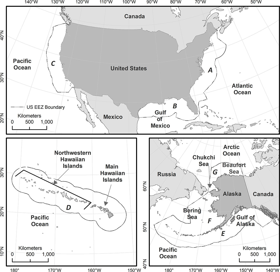
Figure 1 Overview of study area, showing the seven regions within which Biologically Important Areas (BIAs) were assessed. All BIAs evaluated and scored in this effort either fully or partially overlap U.S. waters (i.e., the region shoreward of the offshore boundary of the U.S. Exclusive Economic Zone (EEZ), including state waters); however, BIAs were not truncated at the U.S. EEZ. The seven regions are labeled clockwise starting in the east: (A) East Coast; (B) Gulf of Mexico; (C) West Coast; (D) Hawai’i; (E) Gulf of Alaska; (F) Aleutian Islands and Bering Sea; and (G) Arctic.

2 Methods

The BIA II assessment was a species-focused, science-based process that used expert elicitation and centered on areas that are within, overlap, or are adjacent to U.S. waters. BIAs were delineated based on their importance to a particular species, stock, population, or other ecologically relevant sub-specific identifier. Hereafter, “species” will be used to represent species, stocks, populations, or any other sub-specific unit that has been identified as essential for the identification and/or scoring of a given BIA, as appropriate. BIAs were scored based on detailed written protocols, summarized here (see the Supplementary Material for the complete protocols).

Regional leads with cetacean expertise were chosen to oversee and assist with the identification, delineation, and scoring of BIAs for each of the seven regions. In accordance with the selection process for the initial BIA effort, for BIA II we defined a regional lead as an individual or research group with significant research and technical experience with cetacean species found in a specified region. The regional leads were affiliated with a range of institutions, including academic institutions, governmental agencies, and nongovernmental organizations, including a nonprofit research consortium. Furthermore, to select region leads for BIA II, we gave preference to people who actively participated in or led regional efforts for BIA I.

Regional leads were asked to engage with additional subject matter experts (SMEs) as needed to ensure all available information and necessary expertise were included in the assessment. During an introductory workshop, the BIA II WG leads presented an overview of the purpose, BIA delineation and draft scoring protocols, and schedule for the BIA II effort. Attendees at the introductory workshop included NOAA and Navy project sponsors, regional leads, SMEs, and other interested parties. Workshop participants were encouraged to provide targeted input to help finalize the scoring and labeling protocols. Based on feedback from workshop participants, the WG leads revised the scoring and labeling protocols and subsequently met with the regional leads and SMEs to present the protocols in a comprehensive, step-by-step manner, utilizing case studies to illustrate key scoring and labeling details. An individual (co-author LN) with extensive experience in structured expert elicitation facilitated these early meetings to ensure a shared understanding of the scoring and labeling protocols across regional leads and SMEs. BIA II WG leads held two additional regional check-ins for each region, with participation from regional leads and available SMEs, to answer questions and provide clarity as experts began applying the information assessment and scoring protocols. To promote consistency, notes from the regional check-in meetings were shared across regions. In a few instances, the protocols were revised to address issues that arose in practice. The final protocols, used consistently throughout the BIA II assessment, are provided in the Supplementary Material.

Consistent with BIA I, four types of BIAs were defined for BIA II (Table 1): Reproductive Areas (R-BIA); Feeding Areas (F-BIA); Migratory Routes (M-BIA), and Small and Resident Populations (S-BIA). BIA types are not mutually exclusive. For instance, a species’ feeding BIA might overlap with a migratory BIA in space or time. Small and resident BIAs may encompass both feeding and reproductive areas. Where BIAs span more than one region (a transboundary BIA), region leads worked together to delineate and score the BIA. The associated metadata for a transboundary BIA were compiled by the region that had the largest proportion of the BIA, and the BIA record lists which regions the BIA spans.

TABLE 1

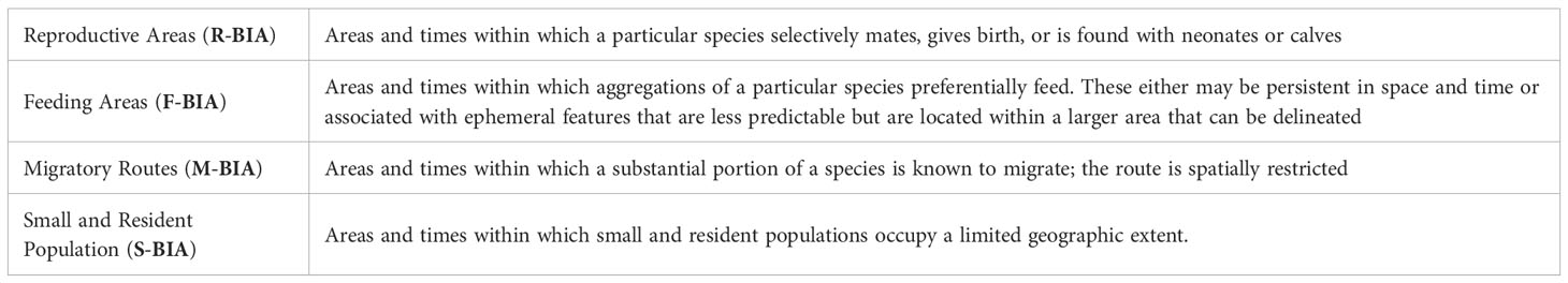
Table 1 Definitions of the four types of Biologically Important Areas (BIAs).

BIA boundaries include only the areas and time periods described in the definitions above (Table 1) based on the information available for the assessment. Habitat suitability predictions alone were insufficient for delineating BIA boundaries. Similarly, BIA boundaries do not include any intentional “buffers” or other precautionary additions of area or time. Last, while we recognize that cetacean distributions and habitat use are undergoing changes and that future changes are predicted due to global stressors such as climate change, evaluating the extent of change to date and predicting changes in the future are outside the scope of the BIA process. BIAs do not consider potential future conditions.

Geographic boundaries may be delineated using a variety of methods, such as geographic features (isobaths, boundaries of bays or inlets, etc.), distances to geographic features, hydrographic features, minimum convex polygons around observation points (e.g., sightings, acoustic detections, or satellite tag locations), polygons surrounding a certain percentage of individuals engaged in a specific activity, etc. BIA boundaries for small and resident populations aim to include 100% of the population. In contrast, boundaries for feeding, reproductive, or migratory BIAs should include less than 100% of the area and time in which the associated activity occurs because these BIAs indicate where a substantial portion of a species “preferentially feeds” or “selectively mates, gives birth, or is found with neonates or calves”, or within which “a substantial portion” is known to migrate (Table 1).

2.1 BIA scoring and labelling protocols

Five metrics were used to score and label BIAs (Table 2). Intensity and Data Support were the two primary scores, upon which the overall Importance score was based. For each candidate BIA, Intensity and Data Support were independently scored utilizing the scoring rules provided for each BIA type (i.e., R-BIA, F-BIA, M-BIA, or S-BIA), which are summarized below. Then, Intensity and Data Support scores were combined to determine an overall Importance score using a single Importance Score matrix for all BIA types (Figure 2). Independently, Boundary Uncertainty and Spatiotemporal Variability (dynamic, ephemeral, or static) were scored for each BIA, using the same rules for all BIA types.

TABLE 2

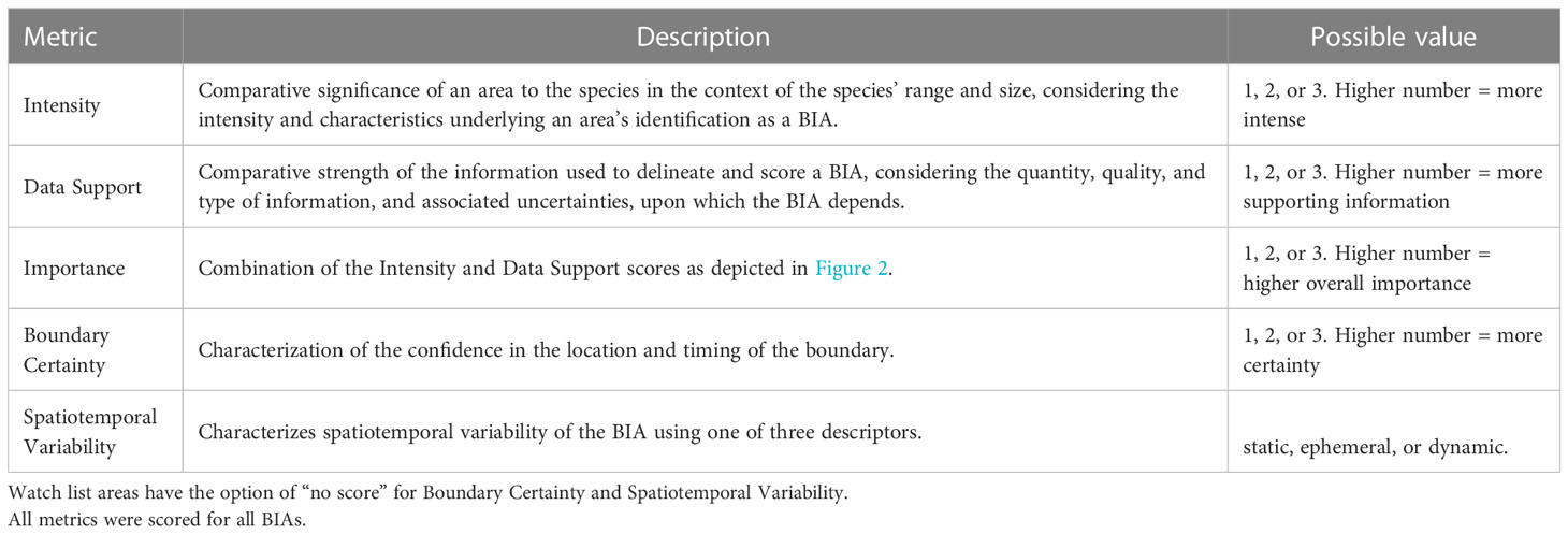
Table 2 Overview of the five BIA scoring metrics.

FIGURE 2

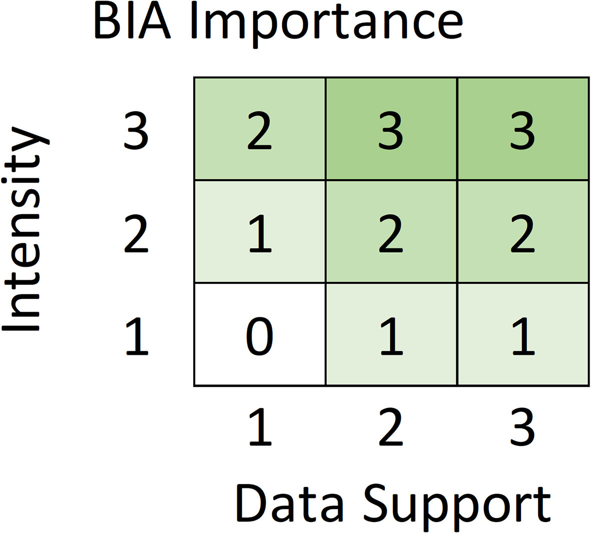
Figure 2 Intensity and Data Support are combined to determine the Importance score for all BIA types based on this Importance matrix.

2.1.1 Intensity scoring

The Intensity score indicates the comparative significance of an area to the species in the context of the BIA type definition and the species’ range and size. This score considers factors such as abundance, density, spatial or temporal extent of use, and proportions, rates, or frequencies of relevant processes (e.g., proportion of the population that uses a migratory corridor; biomass of prey consumed per day; annual use). A higher Intensity score indicates higher values of one or more factors relative to other areas or times, and is associated with more concentrated or focused use. In the context of BIAs, Intensity is based solely on the properties associated with the BIA type description and does not consider other factors such as the health or status of the species, or anthropogenic pressures. Such ancillary factors, when known, may be addressed through other constructs (e.g., Endangered Species Act listing, Potential Biological Removal, Unusual Mortality Events) that users may consider independently of the BIAs. The Intensity score for a BIA may be affected by the number and size of other BIAs of the same type for that species. Although there is no universal rule for adjusting the magnitude of an Intensity score for a given BIA based on the existence of other BIAs, any such consideration is explained in the supporting rationale.

Intensity scoring metrics and rules are different for each BIA type. Intensity was scored entirely quantitatively for S-BIAs and entirely qualitatively for F-BIAs and R-BIAs. Experts could use either an entirely qualitative or partially quantitative approach for M-BIAs.

2.1.1.1 S-BIAs

For S-BIAs, Intensity was quantitatively based on two factors: abundance and range size. For candidate S-BIAs, abundance and range size were first scored independently as 1, 2, or 3 (Table 3). Then, the abundance and range size scores were combined to generate an overall Intensity score using the matrix in Figure 3, which defines the score for all possible combinations of range size and abundance. Populations with abundances above 2000 individuals were not considered qualified as S-BIAs, although there were a few populations where the upper bound of the confidence interval around the abundance exceeded 2000 (and the lower bound was under 2000) that were included. The S-BIA scoring protocols initially included an upper bound for the range size. However, the extent and boundaries of small and resident populations are both influenced by a particular species’ ecology (e.g., some species must range widely to find food, whereas others are able to forage in small areas without ranging widely), and are limited by the availability of the habitat the population relies on. All of the S-BIAs identified are associated with inland or enclosed water bodies (e.g., bays or gulfs), islands or groups of islands, or coastal populations. Given this, limiting populations that may be considered S-BIAs based on a maximum range size was not appropriate, and the scoring protocols were modified to remove the upper limit for range size.

TABLE 3

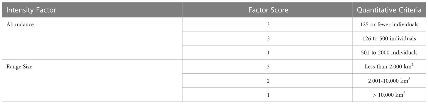
Table 3 Quantitative criteria for scoring abundance and range size factors needed to assign an Intensity score to candidate S-BIAs.

FIGURE 3

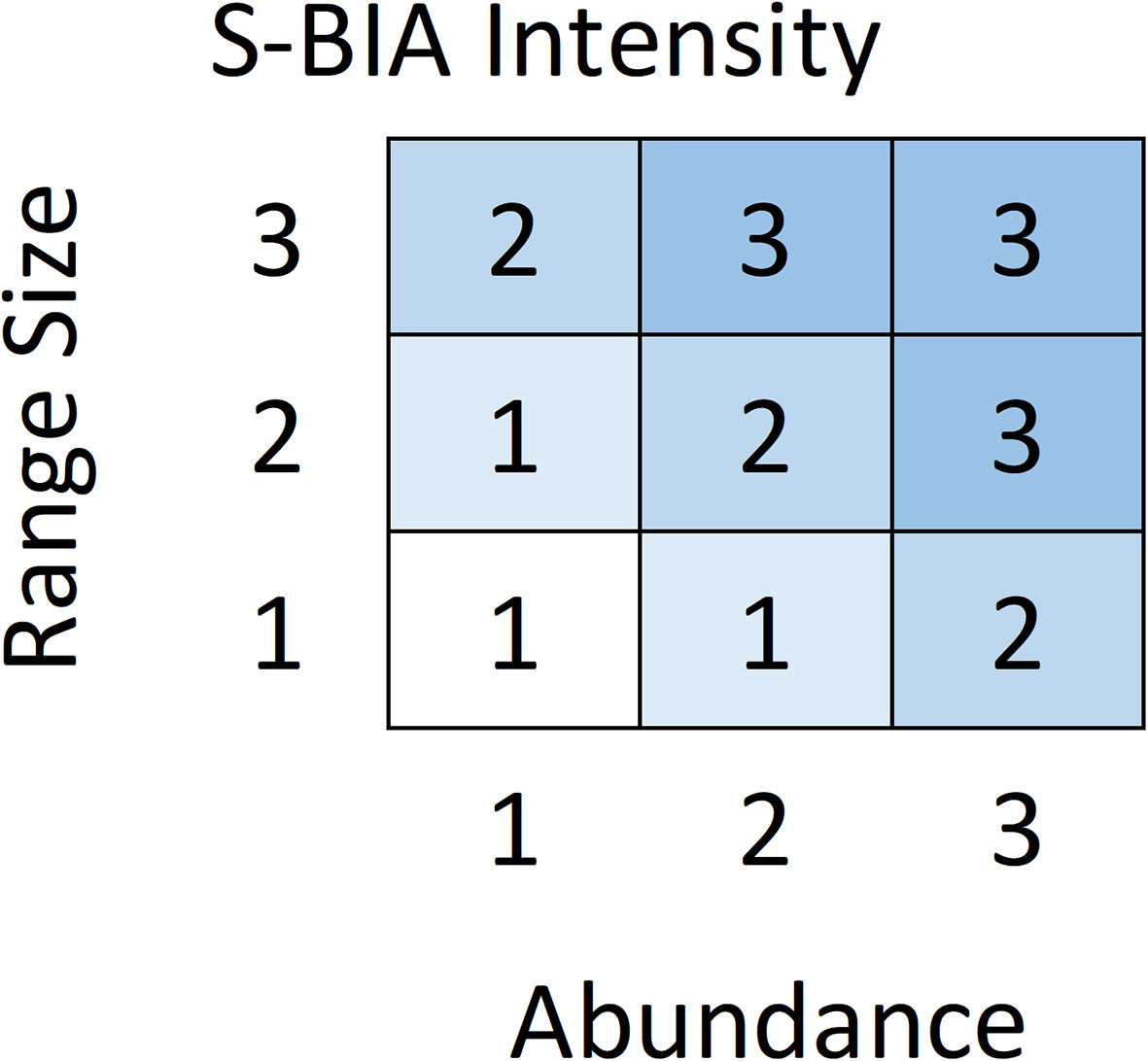
Figure 3 Abundance and range size scores are combined to determine the Intensity score for a candidate S-BIA based on this matrix.

2.1.1.2 F-BIAs and R-BIAs

For F-BIAs and R-BIAs, experts qualitatively considered multiple, but different, Intensity factors (Table 4). The factors vary enough and present enough possible permutations that a strict quantitative scoring system would be challenging to construct for the Intensity score of F-BIAs and R-BIAs. The following scoring rules were applied: (3) indicates high Intensity; (1) represents notably lower Intensity; and (2) represents the remainder of situations that are not notably high or low Intensity. The BIA II WG focused on ensuring consistent logic and scoring across all F-BIAs and R-BIAs for all species, areas, and times through discussions and sharing detailed examples among regions. The rationale for all scores is included in the metadata for each BIA.

TABLE 4

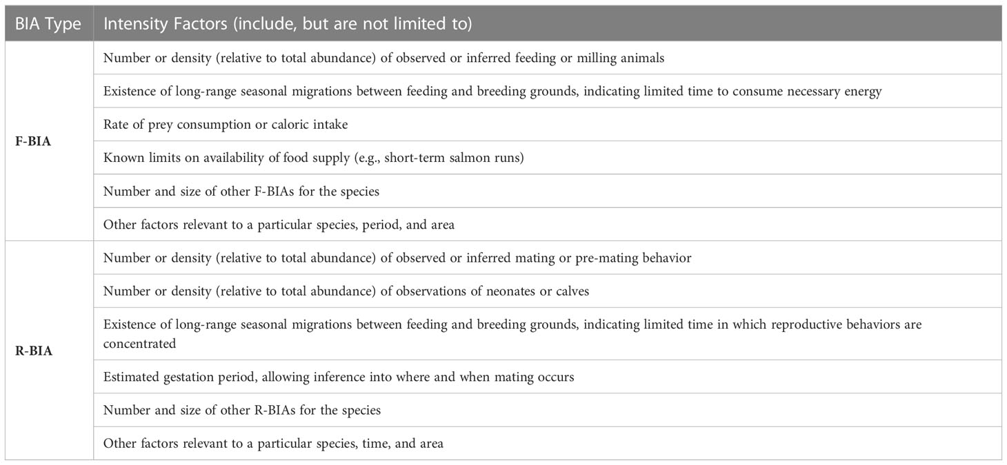
Table 4 Qualitative Intensity factors considered in the Intensity score for F-BIAs and R-BIAs.

The R-BIA definition is tripartite, including areas and times within which a particular species selectively mates, or gives birth, or is found with neonates or calves. We note that a BIA where animals may be “found with neonates or calves” may be distant in space or time from where the animals give birth. This third situation was intentionally included in the definition of an R-BIA to recognize the importance of the presence of comparatively vulnerable younger animals, who may still be learning keys to survival and also receiving nutritional support from their mothers, and the energetic demands on lactating females, among other things. While no firm age limit was initially established for “calves,” discussions with regional leads led to one year being identified as a reasonable bound.

2.1.1.3 M-BIAs

For M-BIAs, experts considered multiple Intensity factors either entirely qualitatively, or with some quantitative consideration (Table 5). Even with some quantitative consideration, the factors vary enough and present enough possible permutations that a strict quantitative scoring system would be challenging to construct for the M-BIA Intensity score. The following scoring rules were applied: (3) indicates high Intensity; (1) represents notably lower Intensity; and (2) represents the remainder of situations that are not notably high or low Intensity.

TABLE 5

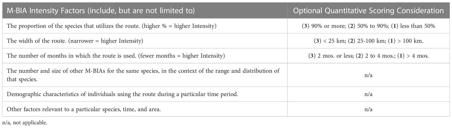
Table 5 Intensity factors that were qualitatively, or partially quantitatively, considered to score M-BIA Intensity.

2.1.2 Data support scoring

The Data Support score is intended to distinguish meaningful differences in the information used to support the identification of and score for the BIA. Supporting information includes Indigenous or local knowledge, community science, raw data, analytical methods, and derived parameters. The scoring of the Data Support metric included consideration of four factors described below: information type, sample size, and quality and uncertainty of supporting information. All Data Support scores were qualitatively determined as described in Table 6.

TABLE 6

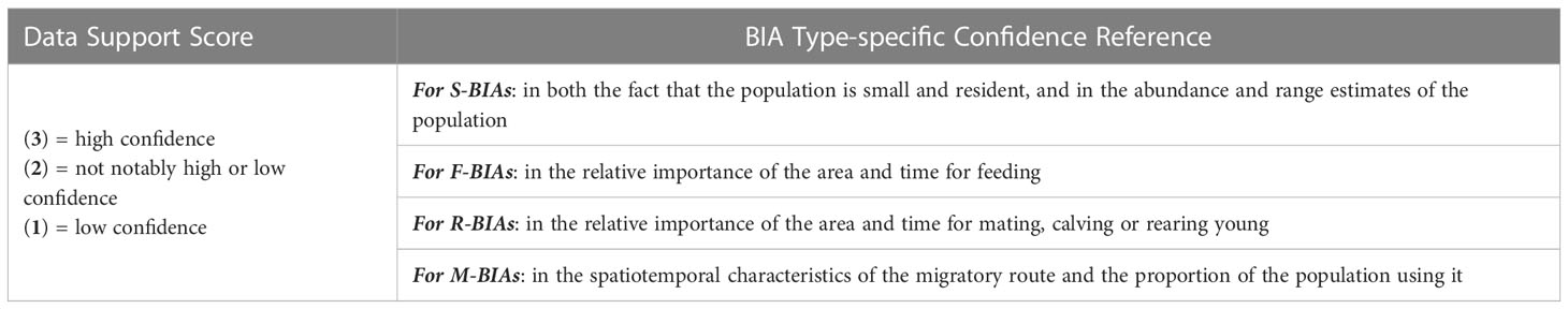
Table 6 The four Data Support score factors of information type, sample size, quality, and uncertainty were qualitatively evaluated to determine a Data Support score for each BIA type as described here.

2.1.2.1 Information types

The different types of information used weigh into the scoring of the Data Support metric. While the applicability of different types of information varies across BIA types, many types of information that could be considered are applicable to multiple types of BIAs and we have provided a general list below. The full BIA protocol document provides more detail regarding the specific types of information these tools can provide and how they may relate to a particular BIA type.

● Indigenous or local knowledge;

● Data from bio-logging tools such as satellite tags, acoustic movement tags, GPS tags, or time-depth tags;

● Photo-identification data;

● Genetic data;

● Line-transect data;

● Passive acoustic recordings and detections; and

● Visual sighting data from systematic marine mammal research, protected species observers for regulated activities, or community science.

2.1.2.2 Sample size

The amount of supporting data, or sample size, weighs into scoring the Data Support metric. Examples of how sample size may be considered include:

● The sample size of bio-logging datasets may be evaluated based on the number and type of tags deployed in different age and sex classes during particular locations and seasons; tag longevity (i.e., the length of the time series from each tag); and the number of years across which the tags were deployed on a particular species.

● Important aspects related to sample size for photo-ID datasets include: number of individuals identified; study duration (in years); spatial and temporal extent of sampling; representativeness of the sample (e.g., age class, sex, proportion of the population with identifiable markings); and the maximum number of years a single individual was identified in an area.

● The sample size of line-transect survey datasets may be evaluated based on the total number of surveys in the time series, total distance (or time) covered on transect, time lag between surveys, and the temporal and spatial extent and resolution (i.e., spacing between transects) of each survey.

● The sample size of passive acoustic monitoring datasets may be evaluated based on the number and location of acoustic recorders, total time sampled, temporal extent of recordings, sample frequency, and number of signals (i.e., calls, whistles, clicks, songs, etc.) of the specific species detected.

● The sample size of visual observation datasets may be evaluated based on the total number of observations, the number of years and months over which the observations were made, and the temporal and spatial extent and resolution of the effort.

2.1.2.3 Quality and uncertainty

Quality and uncertainty represent two different, although related, characteristics. Separate from the amount of supporting information, information can vary in quality. For example, data collected from trained protected species observers (PSOs) conducting a survey to satisfy a regulatory requirement may be more comprehensive or reliable in terms of species identification, group size estimates, time, position, etc., than community science data. Also, the age of information that may be considered relevant for delineating and scoring BIAs may vary by BIA type. For example, regional leads agreed that datasets may remain relevant longer for assessing S-BIAs and M-BIAs because their spatiotemporal boundaries may be unlikely to change over time. In contrast, feeding and activities associated with reproductive success may be more sensitive to changes in the environment; therefore, it may be appropriate to limit data used to delineate and score F-BIAs and R-BIAs to a more recent time period.

Furthermore, analytical methods used to estimate derived parameters vary based on a variety of criteria, including whether the analytical assumptions were appropriate for the data, whether and how correction factors were incorporated to account for known biases in the data, and whether and how uncertainty in derived parameters was estimated. Uncertainty refers to the estimated precision or confidence in derived parameters. Poor quality data may not allow reliable estimates of uncertainty. High quality data that are associated with an inherently noisy system may lead to reliable, yet high, estimates of uncertainty. Lastly, high quality data that have been analyzed poorly will result in unreliable estimates of uncertainty.

To score Data Support, the available information is variable enough, and presents enough possible permutations of type, sample size, quality, and uncertainty that a strict quantitative scoring system (e.g., matrix) would be challenging to construct. Therefore, the qualitative approach described in Table 6 was applied.

2.1.3 Importance score

Intensity and Data Support scores were combined as indicated in the matrix in Figure 2 to determine the overall Importance score. The matrix is designed such that Intensity drives the Importance score except when the Data Support is weakest, in which case the Importance score is lowered by 1. For example, a BIA with an Intensity score of 3 will have an Importance score of 3, except when the Data Support is 1, leading to an Importance score of 2. The Importance Score matrix is identical for all BIA types: Intensity and Data Support each range from 1-3, and the Importance score will always range from 0-3. A zero score was assigned when both Intensity and Data Support were 1, meaning that the area was not considered a BIA at present, but was added to a watch list.

There is one notable exception to the general rule that watch list areas are designated based on Importance scores of zero. Specifically, a candidate S-BIA with Importance score equal to 1 could be added to the watch list, with explicit justification. This exception is necessary because the S-BIA Intensity scoring matrix (Figure 3) does not allow an Intensity score of 1 for populations that fall into the smallest category of either population or range sizes. Consequently, the smallest possible Importance score for this type of candidate S-BIA, based on the Importance matrix (Figure 2), would be 1. If Data Support is sufficiently weak, this type of candidate S-BIA does not qualify to be a BIA and could be designated as a watch list area.

Areas on the watch list may be considered priority areas for future research or for consideration during the next BIA revision. A summary of the areas on the watch list is included in the Assessment section.

2.1.4 Boundary certainty

Boundary Certainty describes the degree of confidence in the location and timing of the BIA boundary. To the extent possible, Boundary Certainty was considered independently of the Intensity, Data Support, and Spatiotemporal Variability (defined below) scores. Boundary Certainty incorporates information about the factors that define the boundary (e.g., bathymetric vs. hydrographic features) and certainty regarding the size, location, and period of occupancy of the BIA. Boundary Certainty should be rated as (1)=low, (2)=medium, or (3)=high. The narrative and metadata explain the boundary characteristics that were used to delineate the boundary and to derive the Boundary Certainty score for each BIA, as well as known limitations (e.g., surveys were conducted within only a limited area or period). All BIAs were assigned a Boundary Certainty score, whereas watch list areas may lack sufficient data to score this metric.

2.1.5 Spatiotemporal variability

Each BIA was assigned a Spatiotemporal Variability indicator (a nominal score). The geographic location of some BIAs may be known, or be highly likely, to vary with time according to some periodicity (i.e., inter-annual, inter-decadal, etc.). Although spatiotemporal variability among different areas exists across a continuum, for the purposes of this exercise, we identify three types of spatiotemporal variability (types derived after Johnson et al., 2018): static, ephemeral, and dynamic.

All BIAs were assigned a Spatiotemporal Variability indicator, whereas watch list areas may lack sufficient information to assign an indicator.

2.1.5.1 Static

A static BIA is characterized by features that are clearly differentiated in the physical world and fixed in space and time (e.g., an island or island chain, a coral reef, seamount, bay, or inlet).

2.1.5.2 Ephemeral

Two types of ephemeral BIAs may be identified. In the first case, more than one BIA subarea may be found within a larger fixed BIA; however, at any given time, not all of the BIA subareas are “active”. In other words, the spatial pattern of the habitat mosaic of BIA subareas within the larger BIA is not static. Each BIA subarea within the habitat mosaic may be activated by a forcing mechanism (e.g., freshwater inflow, upwelling, etc.) that is particular to that subarea. We refer to the spatiotemporal characteristics of such a BIA as ephemeral. The second type of ephemeral BIA is a fixed area that is either entirely “active” or entirely “not active.” An example of this second type of ephemeral BIA is the “krill trap” area near Barrow Canyon in the Arctic region, which was designated as an ephemeral F-BIA in July for bowhead whales (Balaena mysticetus) (Clarke et al., 2023). Furthermore, the BIA may be active according to some periodicity, or it may be aperiodic. For both types of ephemeral BIAs, it is essential to clearly state, if known, the periodicity of the temporal variability and what factors influence the associated variability. The influencing factors may be physical (e.g., water temperature, water mass characteristics, winds, upwelling, freshwater input, hydrographic fronts) or biological (e.g., prey recruitment).

2.1.5.3 Dynamic

A dynamic BIA is associated with persistent but mobile features of the ecosystem, such as major oceanographic fronts. Dynamic BIAs are distinguished from ephemeral BIAs in that the former always exist, but their geographic location varies temporally, whereas ephemeral BIAs may be active or not active.

2.1.6 The BIA “unit” and hierarchical scoring

In the simplest case, a BIA unit corresponds to a single polygon and one continuous period within which a species engages in a particular biologically important activity (i.e., an area that qualifies as a R-, F-, or M-BIA), or it corresponds to the range of a small and resident population. However, it is possible that multiple polygons of the same type of BIA for a species could exist in a single region and period. In that case, it was acceptable and encouraged to identify and score a cluster of BIA polygons as a single unit, regardless of whether they share common boundaries, as long as the scores were identical across all polygons in the cluster.

Also, for this BIA II process, we introduced the concept of “hierarchical” BIAs. Specifically, sometimes high-resolution data are available, and it is appropriate and helpful to reflect a gradation in Intensity score across a larger BIA. Two specific examples are considered. For S-BIAs specifically, there may be a single core area within a larger S-BIA in which the Intensity factors support a higher score (Figure 4). For F-, R-, or M-BIAs, there may be a single area in which a biologically important activity preferentially occurs, yet there may be spatial heterogeneity in Intensity defined by one or more subareas within. These two scenarios are termed “hierarchical scoring”; the larger bounding BIA unit is referred to as the “parent BIA,” and the smaller BIA unit(s) inside are referred to as “child” BIA(s). The scoring described in the methods above is applied to the BIA units in a hierarchical situation; however, additional hierarchical scoring rules apply for different BIA types as described below. Specific information and rationale used to delineate the BIA are explicitly documented in the associated narrative and metadata.

FIGURE 4

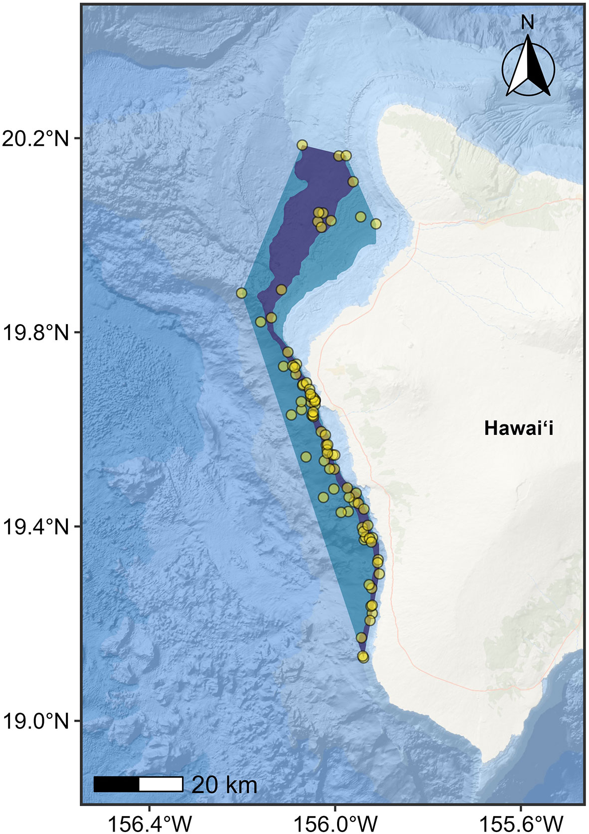
Figure 4 Example of hierarchical small and resident BIA for Hawai’i Island dwarf sperm whale (Kogia sima) (from Kratofil et al., 2023). Parent BIA boundary (blue polygon) for the Hawai‘i Island dwarf sperm whale population represented as a minimum convex polygon (MCP) encompassing all sighting locations in less than 2,000 m water depth (yellow circles), and child BIA boundary (core range; purple polygon) represented as the area between the 500-m and 1,000-m isobaths within the parent BIA. Points are partially transparent to highlight high density areas (i.e., where multiple points overlap). The inner boundary for both BIAs is defined as the 300-m isobath.

2.1.6.1 Hierarchical scoring for R-, F-, and M-BIAs

In the case of R-, F-, and M-BIAs, whether a single core area(s) or multiple child polygon(s), the Intensity score for the parent BIA must be less than the highest Intensity score among the core/child area(s) (Figure 5).

FIGURE 5

Figure 5 Screenshot from the BIA scoring portal depicts part of one of the screens through which regional leads entered the required key characteristics of the BIAs, as well as the supporting rationale.

2.1.6.2 Hierarchical scoring for S-BIAs

S-BIAs are intended to delineate 100% of the species’ range, and quantitative criteria are used to score Intensity. The quantitative criteria for S-BIAs were explicitly designed to apply to a polygon encompassing 100% (or as close as possible given the available information) of the species. Therefore, in a hierarchical situation where it is possible to identify a core area (as in Figure 4), the quantitative criteria described for S-BIAs are applied only to the Intensity of the parent BIA. It is not appropriate to apply the quantitative S-BIA Intensity scoring rules to a child S-BIA (core area). When the quantitative criteria for S-BIAs are applied to the parent, the more intense core child area is accorded a higher Intensity score, unless the parent qualifies for an Intensity of 3, in which case it is impossible to score the child any higher, and the Intensity score for the parent BIA can be equal to the Intensity score for the core/child.

2.1.7 BIA labeling

Each individual BIA unit has a label, which identifies (in order) the BIA type; Importance, Spatiotemporal Variability, and Boundary Certainty scores; region code; identification number; and suffix that indicates hierarchical or non-hierarchical structure. The Intensity and Data Support scores underlying the Importance score are not included in the label but are indicated in the metadata and narratives for each BIA and in the summary tables in the regional manuscripts. The region codes are EC = East Coast, GOM = Gulf of Mexico, WC = West Coast, HI = Hawai‘i, GOA = Gulf of Alaska, ABS = Aleutian Islands and Bering Sea, and ARC = Arctic. For example, a BIA with “R-BIA3-s-b2” at the beginning of the label refers to a Reproductive (R) BIA with the highest (3) of three possible Importance scores, generally static (s) in nature, with medium confidence (b2) in the accuracy of the boundary delineation. For non-hierarchical BIAs, the full label for the BIA would be R-BIA3-s-b2-REG###-0, where “REG” is a placeholder for the region code, “###” represents a sequential identification number that is automatically assigned by the BIA scoring portal (described below), and “0” indicates that it is non-hierarchical. For hierarchical BIAs, each individual (child) BIA unit is represented by a letter following the ID number (e.g., R-BIA3-s-b2-REG###-a); the large (parent) polygon would be labeled in the same way as if it were a non-hierarchical BIA, with the same ID number as the child areas, plus a string of letters representing the child areas it contains (e.g., R-BIA3-s-b2-REG###-0abcde, if it contained 5 child areas).

2.2 Structured expert elicitation

Decision-making is a complex process that becomes even more so when dealing with the marine environment, an intricate and sometimes poorly understood system (Kenchington, 1992; Evans et al., 2017). Collecting more data to improve our knowledge, and hopefully our decision-making as a result, is always an attractive prospect, but does not always account for some factors, such as Indigenous or local knowledge, and human values and behavior (Toomey, 2016); the expected value of the scientific information (Runge et al., 2011); and whether the data will be available on the time scale needed for the decision (Kuhnert et al., 2010). Furthermore, within the context of environmental decision-making, the questions asked are often characterized by limited or highly uncertain data (Kuhnert et al., 2010). Nobody wishes to make uninformed decisions, but waiting for new or improved data to inform the process can result in the loss of opportunities, decisions being made without scientific input, or with the input included in only an ad hoc fashion, such as asking colleagues for their opinions, but failing to capture the wider knowledge of the field.

While the BIA I effort did not suffer from the problem of waiting on data (i.e., BIAs were identified in acknowledgement of the limited information available for some species), reviewers and users identified some concerns, including inconsistencies in how the available information was used to inform the BIAs, and the unintentional exclusion of some information and viewpoints from relevant experts. To rectify these issues, the BIA II WG applied the principles of expert elicitation in a more structured manner for the identification, delineation, and scoring of BIAs.

Expert elicitation is a formal, structured process for obtaining experts’ opinions and knowledge to help inform decision-making, particularly in an information-limited situation. There are many protocols for expert elicitation (e.g., Linstone and Turoff, 1975; Hemming et al., 2017; Gosling, 2018), but all approaches have certain commonalities, such as ensuring that a diverse range of experts is included (e.g., Hemming et al., 2017), aiming to reduce heuristics and biases (e.g., Tversky and Kahneman, 1974), and accounting for the cognitive processes (e.g., Hogarth, 1975) individuals use to interpret the questions they are asked and the information with which they are presented. Another major component of the elicitation process is clear documentation of the methods and judgements so that they can be appraised and the approach considered repeatable (e.g., Hemming et al., 2017). These components directly address the concerns raised in the BIA I effort, and were applied by the BIA II WG in the improved framework for this effort in the following ways:

2.2.1 Wide-ranging information solicitation

The BIA II WG leads first cast a wide net to NOAA scientists and managers, Navy colleagues, and other researchers and BIA users, requesting information regarding opportunities for improvement in the BIA assessment methodology. The BIA II WG leads also asked if there were species or areas that were missing from the BIA I effort or needed revision, and requested relevant supporting information. Regional leads were identified using the criteria listed above and explicitly asked to collaborate with other SMEs, as necessary, to ensure that available information for all taxa, areas, and times were included in the effort.

2.2.2 Extensive communication of purpose, intention, and protocols for BIAs

Prior to and during the scoring process, multiple regional and national workshops were held to ensure that the regional leads and SMEs understood the purpose, intention, and methods for identifying, delineating, and scoring BIAs. These meetings were facilitated and conducted by applying principles of expert elicitation. Particular attention was given to the reduction of linguistic uncertainty to help the experts take a consistent approach to the scoring protocols, and to ensuring all interested parties had the opportunity to contribute their viewpoints and knowledge to the BIA II process. The scoring protocols were explained in detail with scored examples, allowing experts to ask questions to clarify protocols before regional scoring began. Questions and open communication between regional leads, SMEs, and BIA II WG leads were encouraged, in or outside of meetings, and additional topical meetings were held to address specific questions that arose during the scoring effort. Email follow-up and weekly digests summarized important clarifications, decisions, and reminders to keep participants updated and engaged in the knowledge exchange.

2.2.3 Clear documentation of methods

Detailed scoring and labeling protocols were developed and used in this process (see Supplementary Data Sheet 1: A Scoring and Labeling Construct for BIA II). We developed a BIA scoring portal (Figures 5, 6) for region leads that facilitated consistent documentation of key information (e.g., through dropdown menus, must-fill fields) and rationale supporting the BIA delineation and scoring, and further facilitated subsequent review by the BIA II WG leads. This information comprises the metadata included as supplementary materials in each of the regional manuscripts in this special issue.

FIGURE 6

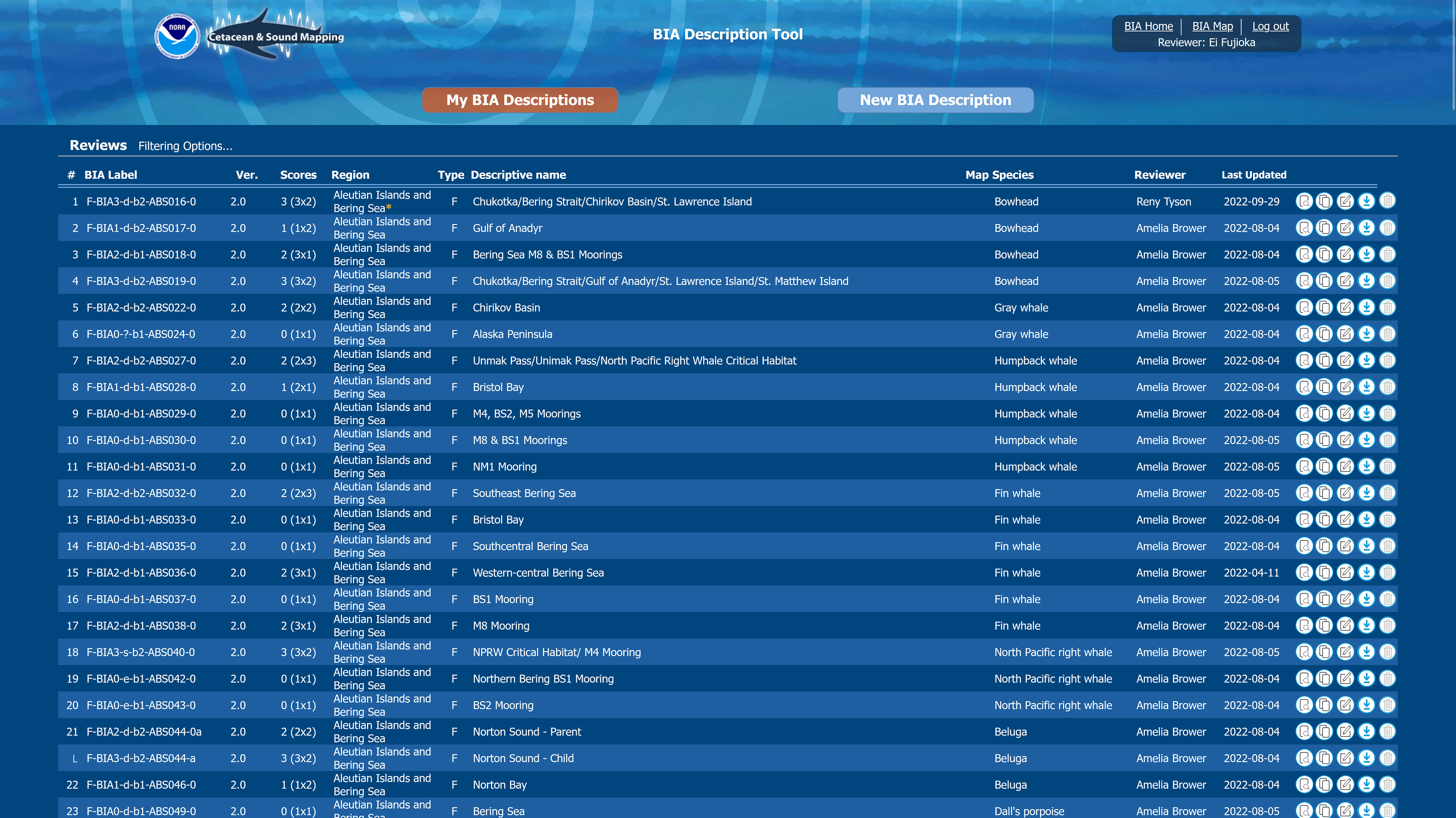
Figure 6 Screenshot from the BIA scoring portal shows the overview page, from which WG reviewers could easily search and access metadata.

2.2.4 Extensive consistency review

Extensive measures were taken to ensure consistent application of the BIA scoring methods across regions and species. In addition to the written protocols, meetings, BIA scoring portal, and communication noted above, three additional steps were taken to maximize consistency. First, early in the scoring stage, regional leads shared examples of scored BIAs representing a variety of BIA types and scores with all other region leads and the BIA II WG leads for review and input. This enabled experts and the facilitation team to identify any inconsistencies across regions, understand the reasons for the discrepancies, and make necessary corrections before the differences permeated the BIA II assessment. Second, after the majority of the BIA scores and supporting rationale were submitted through the BIA scoring portal, the BIA II WG created extensive summary tables and graphics illustrating the differences in scoring, geographic area, and other factors, across regions. These were used to support regional comparisons and highlight factors warranting a closer review, which were then discussed with the region leads, addressed, and corrected, as needed. Lastly, final scores and draft manuscripts were reviewed by the BIA II WG leads and multiple other reviewers from NOAA and the Navy to help ensure no major disparities had been missed or relevant sources of information overlooked.

3 Assessment summary

This BIA assessment identified more than 150¹ BIAs for 25 species (including multiple stocks for some species) within the seven regions, including 32 parent hierarchical BIAs (child BIA numbers not included in the 150+). These BIAs were based on extensive review and synthesis of published and unpublished information by more than 50 SMEs. A summary of the BIAs identified by region, species, and BIA type is provided in Table 7. We note that where data existed to delineate BIAs by month, or half-months, experts were encouraged to do so. For example, the large number of bowhead whale feeding BIAs relative to other species reflects this temporal resolution. Otherwise, the designation of a BIA was year-round. The geographic extent of the BIAs in all regions ranged from 45 km² for one Gulf of Mexico bottlenose dolphin (Tusiops truncatus) small and resident BIA (see LaBrecque et al., In Preparation) to 1,060,171 km² for the minke whale (Balaenoptera acutorostrata) feeding BIA that shares boundaries with the Bering Sea and Arctic regions (see Brower et al., 2022). The best estimates of abundance for the small and resident populations identified across all regions range from 10 (beluga whales (Delphinapterus leucas) in Yakutat Bay, Gulf of Alaska; Wild et al., In Review) to ~4,250 (harbor porpoise (Phocoena phocoena) in Morro Bay; the coefficient of variation values associated with this estimate encompass the largest abundance bin size). The spatial extent of the small and resident populations were as small as 45 km² for the Gulf of Mexico bottlenose dolphin stock mentioned above and as large as 138,000 km² for the Northwestern Hawaiian Islands false killer whale (Pseudorca crassidens) insular stock (see Kratofil et al., 2023).

TABLE 7

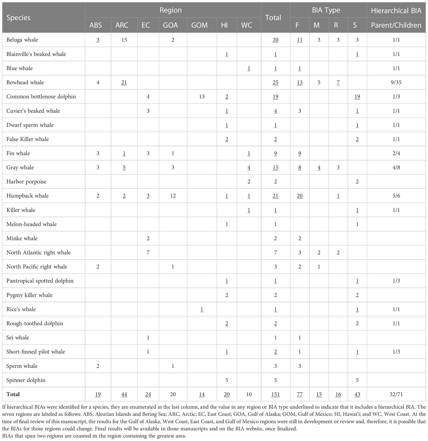
Table 7 BIA counts summarized by region, species, and BIA type.

As noted above, in some instances, information may exist about a species’ use of a particular area and time, but the information was insufficient to confidently delineate a BIA. Specifically, areas for which the Importance score was determined to be zero because both Intensity and Data Support were scored 1 were included in a watch list.² We note that for watch list areas, experts were given the options to not score Boundary Certainty and to not identify a Spatiotemporal Variability indicator (e.g., to enter “no score” in the scoring portal for these two entries). These areas are summarized in Table 8 and may be considered priority areas for future research or for consideration during any future BIA update.

TABLE 8

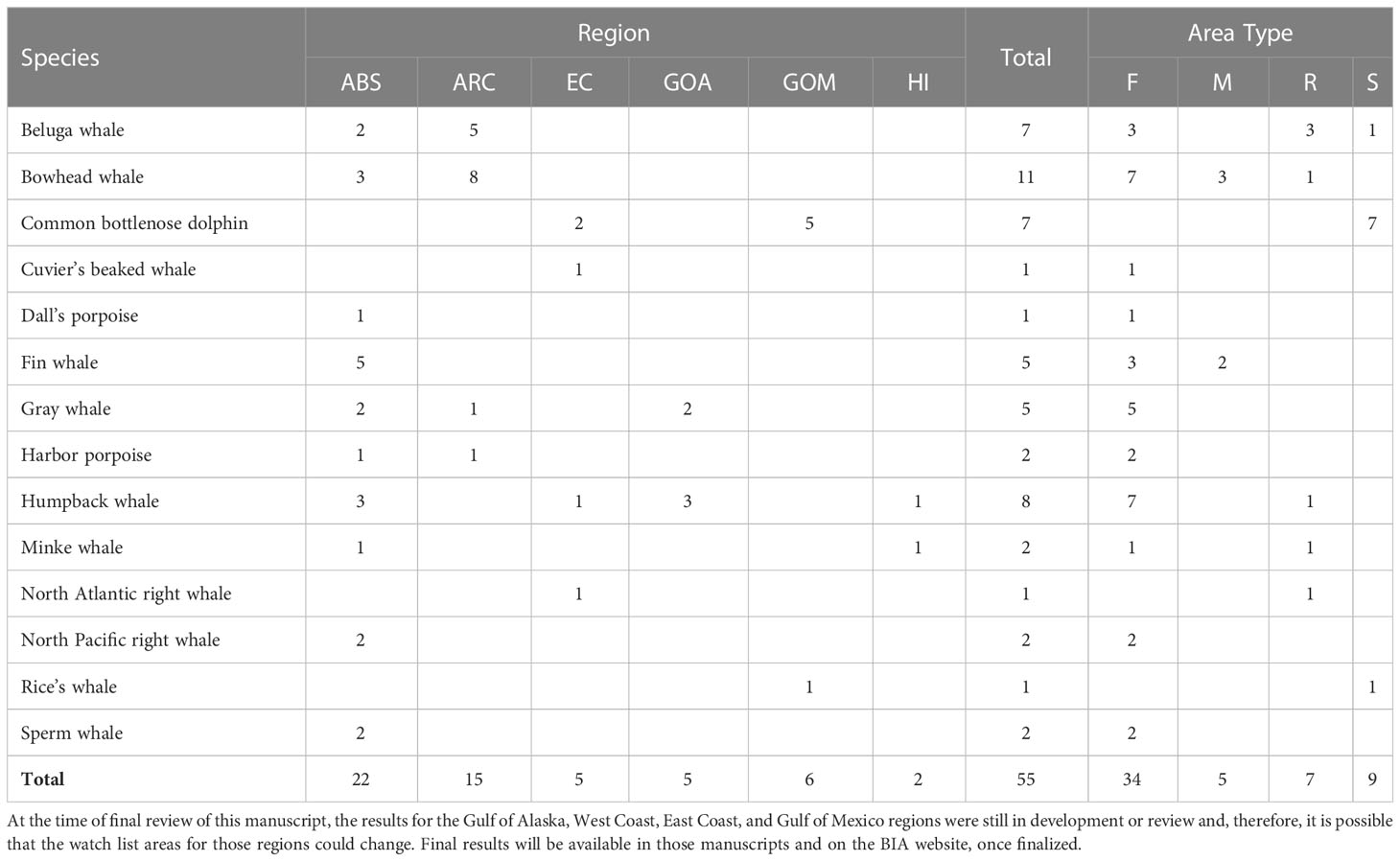
Table 8 Numbers of watch list areas, summarized by region, species, and BIA type.

4 Discussion

4.1 Improvements and opportunities for the BIA II effort

The BIA II WG leads solicited input from experts, including scientists, managers, and users of the BIA I products, in order to improve the quality and value of the BIA products. The expanded information compiled and solicitation methods used in the BIA II effort increased the likelihood that most or all relevant, reliable, and available information was included. The use of a detailed written scoring and labeling construct improves the utility and interpretability of BIAs, allowing managers and users to better compare the importance of BIAs, understand the spatiotemporal variability of a BIA, and understand the level of confidence in the BIA’s spatial and temporal boundaries. Furthermore, the more extensive application of the principles of structured expert elicitation, increased review, and the use of the BIA scoring portal increased consistency in the development of BIAs across regions.

We emphasize here that our goals were to identify where data were available to potentially support the identification of a BIA, and to apply the protocols to delineate and score BIAs where appropriate. Our goal was not to ensure that every species or region has any particular number of BIAs. This effort represents expert judgment applied to the best available information, but that does not mean that every area that qualifies as a BIA has been identified. In fact, there are most certainly BIAs that have not been identified for certain species, especially in areas where less information exists and fewer BIAs have been identified (e.g., the Northwestern Hawaiian Islands). Further, we recognize that in many regions, the areas with the most cetacean data may be areas of management concern due to existing or proposed anthropogenic activities; the greater availability of data leads to a higher likelihood that a BIA could be warranted in those areas, potentially leading to the perception of bias. However, this is not the case. All available information was assessed using a common set of protocols. Regardless of how much information existed, the candidate area had to comport with the BIA definition and scoring rules in order to be delineated as a BIA. For example, a large volume of data for a particular area and time would not warrant a BIA delineation if the information did not demonstrate that a substantial portion of a species migrates through or that cetaceans preferentially feed or selectively mate, give birth, or calve in the area in question. A certain level of information must exist about the species in areas outside the candidate BIA to relate feeding, mating, or reproductive activities inside and outside the candidate area.

The scoring and labeling protocols used in the BIA II effort have provided significant improvements over the BIA I approach, and we have made every effort to ensure consistency in the application of these protocols in the identification, delineation, and scoring across regions and BIAs. Nonetheless, it remains incumbent upon the user to review the metadata and understand the rationale behind the score and boundaries of any BIA in order to appropriately consider the BIA in any assessment or analysis, especially because it is not possible to provide the details of BIA scoring for all areas in the body of each regional manuscript.

Another significant advance in the BIA II effort that reflects user input is the decision not to truncate BIAs at the U.S. Exclusive Economic Zone (EEZ). This modification to the BIA I protocols significantly improves the biological and ecological relevance of the BIAs to any assessment, and expands the total coverage of the effort. However, there is still a need to evaluate the data that may support BIAs that are outside of and not immediately adjacent to the U.S. EEZ (i.e., in the high seas, outside the jurisdiction of any country), and that is a future goal of the BIA II WG. The distant high seas areas could also be coordinated with international Important Marine Mammal Area (IMMA) processes (Tetley et al., 2022), if practical and beneficial.

Another identified opportunity for expansion is to move beyond cetaceans to include BIAs for pinnipeds, or to adapt BIA scoring protocols for other taxa such as fissipeds or sea turtles. BIA protocols could be derived for additional taxa, given additional time, resources, and willing experts.

Lastly, we note that one serious concern for BIA I users, and a recommendation for BIA II, was to ensure that there was the ability to consider and incorporate new information in a timely manner, given the evolving science and changing environment. The process of collecting “all available information,” evaluating potential species, areas, and times, and delineating and scoring BIAs using a thorough structured elicitation process is not trivial. There is no way to easily simplify the process and also retain the rigor. A better goal is to be realistic about workloads and create reasonable timelines for updating BIAs, which will require advance planning for future revision cycles. We believe that approximately every 5 years would be an appropriate target frequency for updating BIAs. However, we fully recognize the importance of incorporating new science into management decisions between updates, and we emphasize the value of assessing the metrics described in the BIA II scoring protocols (e.g., Intensity, Data Support) when considering how to evaluate and weigh new information in the context of the existing BIAs.

4.2 Comparison to international assessments

International efforts to identify important marine areas that meet specific ecological criteria include Ecologically or Biologically Significant Marine Areas (EBSAs; Dunn et al., 2014; Johnson et al., 2018) developed under the Convention on Biological Diversity (CBD), Key Biodiversity Areas (KBAs; International Union for Conservation of Nature (IUCN), 2016), and Important Marine Mammal Areas (IMMAs; IUCN Marine Mammal Protected Areas Task Force, 2018; Tetley et al., 2022). In addition, national efforts such as the Canadian national EBSAs (DFO, 2004; DFO, 2011) and the Australian Biologically Important Areas (Commonwealth of Australia, 2014) provide examples of similar efforts. These place-based approaches were designed to be transparent and provide numerous benefits to taxa, ecosystems, natural resource conservation and management, economics, or society. The primary differences among these place-based assessments include: i) the ecological unit(s) being assessed (i.e., populations, single species, multiple species, species assemblages, communities, or ecosystems); ii) whether socioeconomic factors are considered in addition to ecological factors in the designation criteria; iii) whether the designation criteria are quantitative or qualitative; iv) the finest temporal resolution allowed in delineation; and v) the geographic focus of the overall assessment, all of which affect where candidate areas may be located. We compare NOAA’s BIAs with CBD and Canadian EBSAs, Australian BIAs, KMAs, and IMMAs based on each of these characteristics in turn.

The taxonomic unit considered for NOAA’s BIAs is a cetacean population, stock, species, or other sub-specific taxonomic identification, where applicable. IMMAs delineate areas for one or more marine mammal species, including cetaceans, pinnipeds, sirenians, ursids, and mustelids (IUCN Marine Mammal Protected Areas Task Force, 2018; Tetley et al., 2022). Australian BIAs encompass a broader range of taxa, as they may be delineated for any marine species, but delineation occurs at the level of individual species (Commonwealth of Australia, 2014). Similarly, the CBD and Canadian EBSAs may consider multiple marine taxa, although delineation of an area may be based on a population, species, species assemblage, community, or habitat (DFO, 2004; Dunn et al., 2014; Johnson et al., 2018). KBAs have the broadest taxonomic coverage, applicable to all marine, freshwater, and terrestrial taxa, and may be applied to a population, species, species assemblage, community, or ecosystem (IUCN, 2016).

Similar to NOAA’s BIAs, the Australian BIAs, IMMAs, and EBSAs (both CBD and Canadian) are assessed and delineated based on purely ecological criteria. IMMAs have the most directly comparable criteria (Tetley et al., 2022) and process to NOAA BIAs since these areas are also focused specifically on marine mammals and are developed through the use of expert judgement. Of special note is the parallel focus on reproductive, feeding, and migratory areas as well as resident populations.

In contrast, KBA delineation considers “the relevant aspects of the socio-economic context of the site (e.g., land tenure, political boundaries) in addition to the ecological and physical aspects of the site” (IUCN, 2016). The KBA delineation procedures include these additional criteria because they aim “to derive site boundaries that are ecologically relevant yet practical for management” (IUCN, 2016).

Among the place-based management schemes discussed here, only KBAs have fully quantitative delineation criteria (i.e., thresholds) (IUCN, 2016). There are three main arguments against using quantitative thresholds in the delineation process. First, quantitative thresholds are scale-dependent; therefore, the spatial or temporal scale of the information or assessment will affect the ability of a candidate area to meet a quantitative threshold. Second, quantitative thresholds require quantitative data, which are often not available or are only sparsely available. Lastly, quantitative thresholds could exclude certain types of information, such as Indigenous or local knowledge and community science.

NOAA’s BIA delineation criteria allow delineation at a ½-month resolution. This decision to allow fine-scale temporal resolution in the boundary delineation process is concordant with our guidelines for the spatial domain: NOAA’s BIAs represent areas and times within which activities are known to occur; addition of temporal or spatial buffers may occur at a subsequent step in an impact analysis. Australian BIAs and EBSAs (CBD and Canadian) also allow boundary delineation by month. In contrast, IMMAs and KBAs do not explicitly discuss temporal extent or variability.

Waters inshore of the U.S., Canadian, and Australian EEZ are the focus of the NOAA, Canadian, and Australian BIAs, respectively, though U.S. BIAs may also extend beyond, or be adjacent to, EEZ boundaries. IMMAs and CBD EBSAs may be delineated in all areas of the oceans, irrespective of national jurisdiction. KBAs are also global, and they may be terrestrial, freshwater, or marine.

5 Conclusion

BIAs are one in a growing international collection of tools created to assist multiple entities in the characterization, analysis, and minimization of anthropogenic impacts on cetaceans, other taxa, and ecosystems. All of the tools require regular review and revision to track emerging knowledge and understanding about the species and ecosystems, as well as anthropogenic pressures, of concern. Communication among those overseeing each assessment process will be critical in order to share limited resources (i.e., time, money, and knowledge) and to enhance understanding of how the products from each assessment can be integrated and used.

BIAs are intended as a synthesis of best available science related to cetacean small resident populations and areas and times selectively used for fundamentally important activities, including feeding, reproduction, and migration. As described above, BIAs can be used as needed to inform impact analyses, planning, or the development of protective measures, where appropriate. BIAs are defined and scored to only reflect the best available information and intentionally do not include any buffers or other precautionary adjustments. In this way, this BIAs are useful for analytical purposes and a variety of management purposes. For example, if a BIA is being used to support a protective measure for a particular stressor or activity pursuant to a particular regulatory requirement, managers can use the BIAs, in whole or in part, with or without different sized buffers, as appropriate given the specific circumstances, rather than assuming that one particular application or pre-applied “precautionary buffer” is suitable for every situation.

Evidence continues to mount to show the importance of the information contained in BIAs in order to understand and address the impacts of anthropogenic activities on cetaceans. The development of the new scoring and labeling protocols in BIA II are a fundamental advancement that improve the utility of the BIAs by allowing users to more clearly differentiate between key characteristics of different BIAs, which in turn allows for more refined application of the BIAs in assessments to support environmental planning, compliance, and protection.

Data availability statement

The original contributions presented in the study are included in the article/Supplementary Material. BIA II interactive maps and associated metadata, as well as the regional article, will be available on the NMFS website (https://oceannoise.noaa.gov/biologically-important-areas). Further inquiries can be directed to the corresponding author.

Author contributions

All co-authors were members of the BIA II working group and planning team. JH and MF developed the BIA II scoring protocols, oversaw the development of regional BIAs, and led the writing of the draft manuscript. LN facilitated the expert elicitation process. JC, SD, EF, CC, and PH developed the BIA II data portal, and provided technical support including with the creation of BIA boundaries and figures. RTM and SVP facilitated the development of regional BIAs, and contributed to the development and application of the BIA II scoring protocols. All co-authors contributed to writing and editing the manuscript, and approved the submitted version.

Funding

This work was completed through a collaboration between NOAA and the U.S. Navy to better describe areas and time periods in which cetacean populations are known to concentrate for breeding, feeding, and migration, and areas within which small and resident populations occupy a limited geographic extent.

Acknowledgments

We thank all region leads and subject matter experts who provided input and data to delineate BIAs during this effort, including: Jason Allen, Helen Bailey, Robin Baird, Brian Balmer, Kim Bassos-Hull, Elizabeth Becker, Amanda Bradford, Amelia Brower, John Calambokidis, Emily Chou, Janet Clarke, Carolyn Cush, Genevieve Davis, Annamaria DeAngelis, Kristi Fazioli, Heather Foley, Karin Forney, Christine Gabriele, Annette Harnish, Brad Hanson, Elli Haywood, Elliott Hazen, Elizabeth Henderson, Stefanie Gazda, Annie Gorgone, Jeremy Kiszka, Michaela Kratofil, Erin LaBrecque, Barbara Laquerquist, Kate Lomac-MacNair, Steven Martin, Sabre Mahaffy, Vanessa Mintzer, John Moran, Anita Murray, Janet Neilson, Erin Oleson, Daniel Palacios, Heidi Christine Pearson, Ester Quintana-Rizzo, Melinda Rekdahl, Meghan Rickard, Heather Riley, Jooke Robbins, Cotton Rockwood, Errol Ronje, Howard Rosembaum, Greg Schorr, Julie Stepanuk, Andy Szabo, Leslie Thorne, Christina Toms, Danielle Waples, Lauren Wild, Randy Wells, and Anne Zoidis. We also thank the U.S. Navy, specifically Danielle Kitchen, Ben Colbert, Mandy Shumaker, and Anu Kumar, and NMFS staff for their review and input on the BIA delineations and manuscripts.

Conflict of interest

RTM is employed by Ocean Associates, Inc.

The remaining authors declare that the research was conducted in the absence of any commercial or financial relationships that could be construed as a potential conflict of interest.

Publisher’s note

All claims expressed in this article are solely those of the authors and do not necessarily represent those of their affiliated organizations, or those of the publisher, the editors and the reviewers. Any product that may be evaluated in this article, or claim that may be made by its manufacturer, is not guaranteed or endorsed by the publisher.

Author disclaimer

The views expressed here are those of the authors and do not necessarily reflect the views of the U.S. National Marine Fisheries Service, NOAA.

Supplementary material

The Supplementary Material for this article can be found online at: https://www.frontiersin.org/articles/10.3389/fmars.2023.1081893/full#supplementary-material

We include the Scoring and Labeling Construct for BIA II that was provided to Regional Leads to guide their identification, delineation, scoring, and labeling of BIAs. A few modifications have been made to reflect changes identified and discussed through the course of the effort.

Footnotes

1. ^ At the time of publication, 151 BIAs had been identified (not counting children); however, a few regions were still in the process of review, and numbers could potentially change.
2. ^ As described in the “Importance Score” section above, there is one exception to this, wherein a candidate S-BIA with Importance score equal to 1 could be added to the watch list, with explicit justification.

References

Brower A., Ferguson M., Clarke J., Fujioka E., DeLand S. (2022). Biologically Important Areas II for cetaceans within U.S. and adjacent waters – Aleutian Islands and Bering Sea Region. Front. Mar. Sci. 9. doi: 10.3389/fmars.2022.1055398

CrossRef Full Text | Google Scholar

Clarke J. T., Ferguson M. C., Brower A. A., Fujioka E., DeLand S. (2023). Biologically Important Areas II for cetaceans within U.S. and adjacent waters – Arctic region. Front. Mar. Sci. 10. doi: 10.3389/fmars.2023.1040123

CrossRef Full Text | Google Scholar

Commonwealth of Australia (2014). Protocol for creating and updating maps of biologically important areas of regionally significant marine species. 12. Available at: https://www.dcceew.gov.au/sites/default/files/documents/bia-protocol.pdf.

Google Scholar

de Vere A. J., Lilley M. K., Frick E. E. (2018). Anthropogenic impacts on the welfare of wild marine mammals. Aquat. Mammals 44 (2), 150–180. doi: 10.1578/AM.44.2.2018.150

CrossRef Full Text | Google Scholar

DFO (2011). Identification of ecologically and biologically significant areas (EBSAs) in the Canadian Arctic. DFO Can. Sci. Advis. Sec. Sci. Advis. Rep. 2011/055. Available at: https://waves-vagues.dfo-mpo.gc.ca/library-bibliotheque/344747.pdf.

Google Scholar

Division of Fisheries and Oceans Canada [DFO] (2004). “Identification of ecologically and biologically significant areas,” in DFO can. sci. advis. sec. ecosystem status rep. 2004/006, 15. Available at: https://waves-vagues.dfo-mpo.gc.ca/library-bibliotheque/314806.pdf.

Google Scholar

Duarte C. M., Chapuis L., Collin S. P., Costa D. P., Devassy R. P., Eguiluz V. M., et al. (2021). The soundscape of the anthropocene ocean. Science 371 (6529), eaba4658. doi: 10.1126/science.aba4658

CrossRef Full Text | Google Scholar

Dunlop R. A., Braithwaite J., Mortensen L. O., Harris C. M. (2021). Assessing population-level effects of anthropogenic disturbance on a marine mammal population. Front. Mar. Sci 8. doi: 10.3389/fmars.2021.62498

CrossRef Full Text | Google Scholar

Dunn D. C., Ardron J., Bax N., Bernal P., Cleary J., Cresswell I., et al. (2014). The convention on biological diversity’s ecologically or biologically significant areas: origins, development, and current status. Mar. Policy 49, 137–145. doi: 10.1016/j.marpol.2013.12.002

CrossRef Full Text | Google Scholar

Evans M. C., Davila F., Toomey A., Wyborn C. (2017). Embrace complexity to improve conservation decision making. Nat. Ecol. Evol. 1 (11), 1588–1588. doi: 10.1038/s41559-017-0345-x

CrossRef Full Text | Google Scholar

Ferguson M. C., Curtice C., Harrison J., Van Parijs S. M. (2015). 1. Biologically Important Areas for cetaceans within U.S. waters - overview and rationale. Aquat. Mammals 41 (1), 2–16. doi: 10.1578/AM.41.1.2015.2

CrossRef Full Text | Google Scholar

Gosling J. P. (2018). “SHELF: The Sheffield elicitation framework,” in Elicitation (Cham: Springer), 61–93.

Google Scholar

Gouveia D., Almunia C., Cogne Y., Pible O., Degli-Esposti D., Salvador A., et al. (2019). Ecotoxicoproteomics: A decade of progress in our understanding of anthropogenic impact on the environment. J. Proteomics 198, 66–77. doi: 10.1016/j.jprot.2018.12.001

CrossRef Full Text | Google Scholar

Hemming V., Burgman M. A., Hanea A. M., McBride M. F., Wintle B. C. (2017). A practical guide to structured expert elicitation using the IDEA protocol. Methods Ecol. Evol. 9 (1), 169–180. doi: 10.1111/2041-210X.12857

CrossRef Full Text | Google Scholar

Hogarth R. M. (1975). Cognitive processes and the assessment of subjective probability distributions. J. Am. Stat. Assoc. 70 (350), 271–289. doi: 10.1080/01621459.1975.10479858

CrossRef Full Text | Google Scholar

ICUN Marine Mammal Protected Areas Task Force. (2018) Guidance on the use of selection criteria for the identification of important marine mammal areas (IMMAs). Available at: https://www.marinemammalhabitat.org/download/guidance-on-the-use-of-selection-criteria-for-the-identification-of-important-marine-mammal-areas-immas/.

Google Scholar

International Union for Conservation of Nature [IUCN] (2016). “),” in A global standard for the identification of key biodiversity areas, version 1.0, 1st ed. (Gland, Switzerland: IUCN). Available at: https://portals.iucn.org/library/sites/library/files/documents/Rep-2016-005.pdf.

Google Scholar

Johnson D., Barrio Frojan C., Dunn D., Weaver P., Gunn V., Turner P., et al. (2018). Reviewing the EBSA process: Improving on success. Mar. Policy 88, 75–85. doi: 10.1016/j.marpol.2017.11.014

CrossRef Full Text | Google Scholar

Keen K. A., Beltran R. S., Pirotta E., Costa D. P. (2021). Emerging themes in population consequences of disturbance models. Proc. R. Soc. B288. 20210325. doi: 10.1098/rspb.2021.0325

CrossRef Full Text | Google Scholar

Kenchington R. A. (1992). Decision making for marine environments. Mar. pollut. Bull. 24 (2), 69–76. doi: 10.1016/0025-326X(92)90732-L

CrossRef Full Text | Google Scholar

Kratofil M., Harnish A. E., Mahaffy S. D., Henderson E. E., Bradford A. L., Martin S. W., et al. (2023). Biologically Important Areas II for cetaceans within U.S. and adjacent waters – Hawai‘i Region. Front. Mar. Res. 10. doi: 10.3389/fmars.2023.1053581

CrossRef Full Text | Google Scholar

Kuhnert P. M., Martin T. G., Griffiths S. P. (2010). A guide to eliciting and using expert knowledge in Bayesian ecological models. Ecol. Lett. 13 (7), 900–914. doi: 10.1111/j.1461-0248.2010.01477.x

CrossRef Full Text | Google Scholar

LaBrecque E., Tyson Moore R. B., Gorgone A., Ronje E., Gazda S., Allen J., et al. Biologically Important Areas II for cetaceans within U.S. and adjacent waters – Gulf of Mexico Region. Front. Mar. Sci. (In Preparation).

Google Scholar

Lettrich M. D., Asaro M. J., Borggaard D. L., Dick D. M., Griffis R. B., Litz J. A., et al. (2019). A method for assessing the vulnerability of marine mammals to a changing climate. United States: National Marine Fisheries Service. Office of Science and Technology. NOAA tech. memo. NMFS-F/SPO; 196. doi: 10.25923/7rck-gp41

CrossRef Full Text | Google Scholar

Linstone H. A., Turoff M. (1975). The delphi method (Addison-Wesley: Reading, MA), 3–12.

Google Scholar

McHuron E. A., Schwarz L. K., Costa D. P., Mangel M. (2018). A state-dependent model for assessing the population consequences of disturbance on income-breeding mammals. Ecol. Model. 385, 133–144. doi: 10.1016/j.ecolmodel.2018.07.016

CrossRef Full Text | Google Scholar

National Research Council (NRC) (2005). Marine mammal populations and ocean noise (Washington, DC: National Academies Press).

Google Scholar

New L. F., Clark J. S., Costa D. P., Fleishman E., Hindell M. A., Klanjšek T., et al. (2014). Using short-term measures of behaviour to estimate long-term fitness of southern elephant seals “Tracking fitness in marine vertebrates” theme section. Mar. Ecol. Prog. Ser. 469, 99–108. doi: 10.3354/meps10547

CrossRef Full Text | Google Scholar

New L., Lusseau D., Harcourt R. (2020). Dolphins and boats: When is disturbance, disturbing? Front. Mar. Sci. doi: 10.3389/fmars.2020.00353

CrossRef Full Text | Google Scholar

O’Hara C. C., Frazier M., Halpern B. S. (2021). At-Risk marine biodiversity faces extensive, expanding, and intensifying human impacts. Science 372 (6537), 84–87. doi: 10.1126/science.abe6731

CrossRef Full Text | Google Scholar

Pirotta E., Booth C. G., Cade D. E., Calambokidis J., Costa D. P., Fahlbusch J. A., et al. (2021). Context-dependent variability in the predicted daily energetic costs of disturbance for blue whales. Conserv. Physiol. 9 (1), coaa137. doi: 10.1093/conphys/coaa137

CrossRef Full Text | Google Scholar

Pirotta E., Booth C. G., Calambokidis J., Costa D. P., Fahlbusch J. A., Friedlaender A. S., et al. (2022). From individual responses to population effects: Integrating a decade of multidisciplinary research on blue whales and sonar. Anim. Conserv 25, 796–810. doi: 10.1111/acv.12785

CrossRef Full Text | Google Scholar

Poeta G., Staffieri E., Acosta A. T., Battisti C. (2017). Ecological effects of anthropogenic litter on marine mammals: A global review with a “black-list” of impacted taxa. Hystrix 28 (2), 253. doi: 10.4404/hystrix-00003-2017

CrossRef Full Text | Google Scholar

Roberts J. J., Best B. D., Mannocci L., Fujioka E. I., Halpin P. N., Palka D. L., et al. (2016). Habitat-based cetacean density models for the US Atlantic and Gulf of Mexico. Sci. Rep. 6 (1), 1–12. doi: 10.1038/srep22615

CrossRef Full Text | Google Scholar

Runge M. C., Converse S. J., Lyons J. E. (2011). Which uncertainty? Using expert elicitation and expected value of information to design an adaptive program. Biol. Conserv. 144 (4), 1214–1223. doi: 10.1016/j.biocon.2010.12.020

CrossRef Full Text | Google Scholar

Sherman K., Alexander L. M. (1986). Variability and management of large marine ecosystems (AAAS selected symposium 99) (Boulder, CO: Westview Press).

Google Scholar

Southall B. L., Nowacek D. P., Bowles A. E., Senigaglia V., Bejder L., Tyack P. L. (2021). Marine mammal noise exposure criteria: Assessing the severity of marine mammal behavioral responses to human noise. Aquat. Mammals 47 (5), 421–464. doi: 10.1578/AM.47.5.2021.421

CrossRef Full Text | Google Scholar

Tetley M. J., Braulik G. T., Lanfredi C., Minton G., Panigada S., Politi E., et al. (2022). The important marine mammal area network: A tool for systematic spatial planning in response to the marine mammal habitat conservation crisis. Front. Mar. Sci. 9. doi: 10.3389/fmars.2022.841789

CrossRef Full Text | Google Scholar

Toomey A. H. (2016). What happens at the gap between knowledge and practice? spaces of encounter and misencounter between environmental scientists and local people. Ecol. Soc. 21 (2), 28. doi: 10.5751/ES-08409-210228

CrossRef Full Text | Google Scholar

Tversky A., Kahneman D. (1974). Judgment under uncertainty: Heuristics and biases: Biases in judgments reveal some heuristics of thinking under uncertainty. Science 185 (4157), 1124–1131. Available at: https://www.jstor.org/stable/1738360.

Google Scholar

Van Parijs S. M. (2015). Letter of introduction to the Biologically Important Areas. Aquat. Mammals 41 (1), 1. doi: 10.1578/AM.41.1.2015.1

CrossRef Full Text | Google Scholar

Wild L. A., Riley H. E., Pearson H. C., Gabriele C. M., Neilson J. L., Szabo A., et al Biologically Important Areas II for cetaceans within U.S. and adjacent waters – Gulf of Alaska Region. Front. Mar. Sci. (In Review).

Google Scholar