Impact of satellite and regional in-situ profile data assimilation on a high-resolution ocean prediction system in the Northwest Pacific

1 Introduction

The Northwest Pacific (NWP) has a complicated ocean circulation system consisting of several major currents including the North Equatorial Countercurrent, Subtropical Countercurrent, Oyashio current (OYC), and the Kuroshio Current (Figure 1). The Kuroshio current is a strong western boundary current, accompanied by energetic variability associated with mesoscale features such as eddies and meander. In addition, four major marginal seas, the South China Sea (SCS), the East China Sea, the Yellow Sea, and the East/Japan Sea (EJS), are connected by four narrow straits: Taiwan, Korea/Tsushima, Tsugaru, and Soya Strait. As ocean currents between the marginal seas distribute heat, salt, and other material through straits, it is important to determine the circulation and variability in the marginal seas and their relation to each other and the NWP (Cho et al., 2009). The Korea Institute of Ocean Science and Technology (KIOST) has developed the Korea Operational Oceanographic System–Ocean Predictability Experiment for Marine environment (KOOS-OPEM, Park et al., 2010; Kim et al., 2021), a high-resolution ocean prediction system for the NWP ocean, to understand the complicated ocean circulation system of the NWP ocean and the relationship between the marginal seas and the NWP and to rapidly respond to extreme marine events and accidents.

FIGURE 1

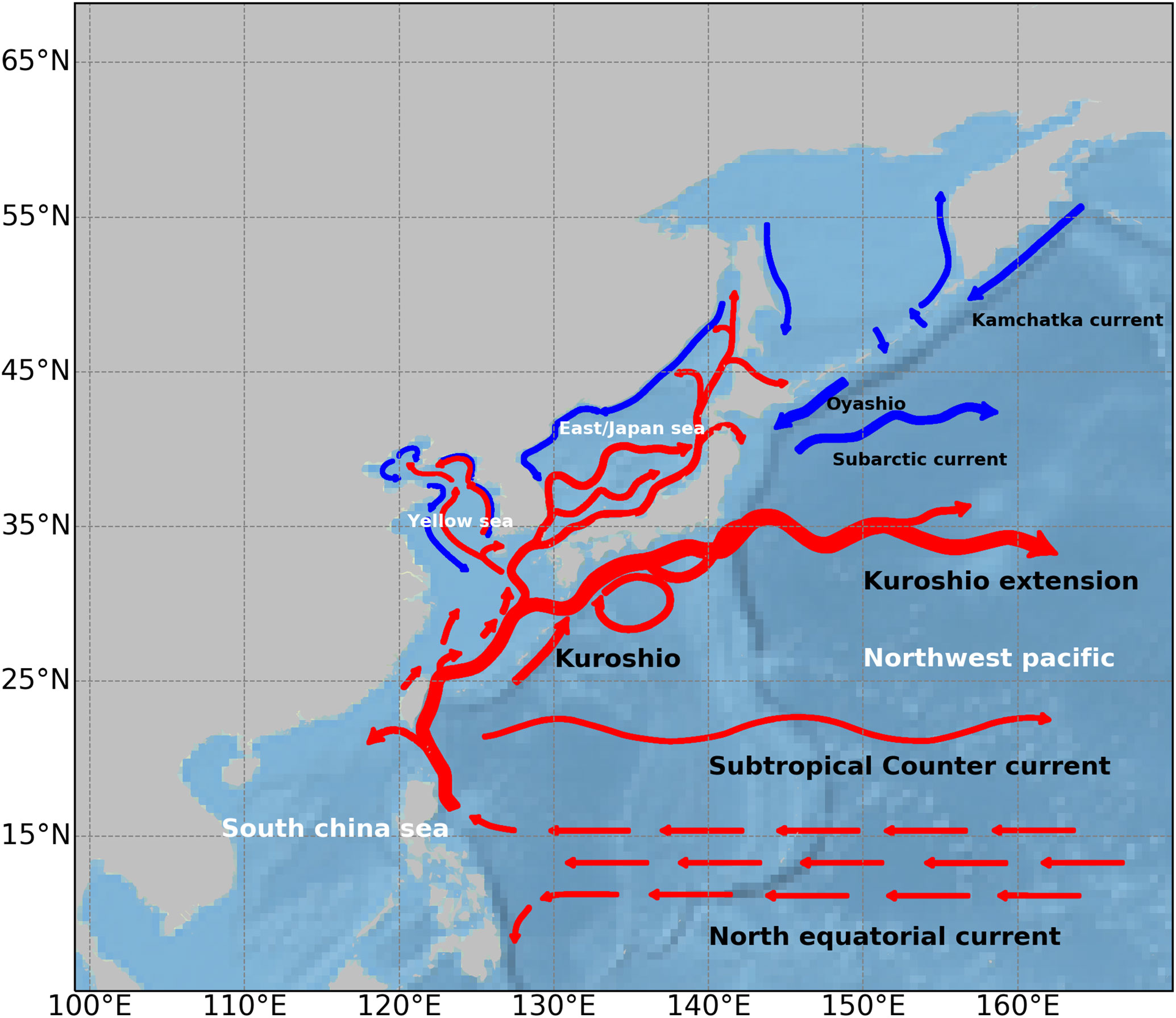
Figure 1 Ocean current map in Northwest pacific is from Park et al. (2013).

Ocean models are imperfect and inevitable sources of uncertainties, such as initial and boundary conditions, model parameterization, and force fields, which may affect their outputs. An efficient strategy to address these uncertainties and improve forecasts is to assimilate available satellite and in-situ observation data into ocean models, thereby optimizing the initial conditions of the ocean model. Generally, data assimilation techniques are classified into two types: variational and sequential. One of the most commonly used variational methods is 4D-VAR whereas the Ensemble Kalman Filter (EnKF), introduced by Evensen (1994) and Burgers et al. (1998), is the most commonly used sequential method. However, these methods are limited because they are computationally expensive. Therefore, the ensemble optimal interpolation (EnOI), a simplification of the EnKF method, was proposed by Evensen (2003) and provides a cost-effective alternative to the EnKF. EnOI estimates the background error covariance by using a time-invariant ensemble of model states sampled from long-term model results. EnOI has many advantages, such as inherent multivariate, quasi-dynamically consistent, inhomogeneous, and anisotropic covariance. Accordingly, EnOI has been adopted in many operational ocean forecast systems, such as the data assimilation system of KIOST (DASK, Kim et al., 2015) and Bluelink Ocean Data Assimilation System (BODAS, Oke et al., 2008).

Traditionally, observational data used in ocean data assimilation include sea surface temperature (SST), temperature/salinity (T/S) profiles, and sea surface height (SSH) derived from satellite altimetry data. SST observations have been widely used in ocean data assimilation because SST is an important ocean variable that connects many processes, such as the air-sea exchange of energy and the formation of water mass in the upper ocean. The assimilation of the T/S profiles improves the representation of seawater density, indicating the mass of water. In particular, the profiles directly affect the ocean heat content (Zhou et al., 2021). The assimilation of SSH improves the ocean surface currents. In addition, these data can reflect the state of the subsurface structure, which provides a physical foundation for improving the temperature and salinity structures of ocean prediction models via assimilation (Troccoli and Haines, 1999). However, it is difficult to project satellite altimetry data onto subsurface density structures. In addition, because the assimilation of satellite altimetry data does not impose constraints on the vertical density structure, consistent adjustments of temperature/salinity should be considered to maintain the density structure. However, when the temperature changes due to the assimilation of satellite altimetry data, adjustment of salinity is required to conserve the correct density stratification (Troccoli et al., 2002; Vialard et al., 2003). Therefore, if the data assimilation system is not properly applied, the assimilation of satellite altimetry data can negatively affect the salinity field while improving the temperature (Fu and Zhu, 2011).

Various methods have been proposed to address these problems and effectively assimilate satellite altimetry data. For example, the direct assimilation method for satellite altimetry data using ensemble-based techniques (Parent et al., 2003; Testut et al., 2003; Birol et al., 2005; Oke et al., 2008; Counillon and Bertino, 2009; Zheng and Zhu, 2015) achieved the projection of surface information onto subsurface structures through the inherent multivariate relation derived from the ensembles. Yan et al. (2004) have proposed an assimilation method based on 3D-VAR by developing a statistical relationship between the SSH and the subsurface structure of temperature and salinity. Cooper and Haines (1996) (hereafter CH96) applied the conservation principle to project altimetry information into subsurface structures. CH96 derived pseudo-profiles based on the rearrangement of the preexisting water columns of the model while preserving the water properties. The pseudo-profiles at the specific grid points are constructed by vertically replacing the preexisting profile, which reduces the surface pressure difference between the modeled and observed SSH with conserving the bottom pressure.

In this study, to quantitatively evaluate the contribution of in-situ T/S profiles and satellite observation data, such as SST and satellite altimetry, to the ocean prediction system, we conducted a sensitivity experiment by applying EnOI to KOOS-OPEM. El-Geziry and Bryden (2010) stated that Mediterranean circulation affects not only the Mediterranean basin on a regional scale but also the global circulation due to its effective contribution to the North Atlantic circulation system. Like the Mediterranean Sea, the EJS is a semi-enclosed marginal sea exchanging water mass with the open ocean through narrow straits. This study also aimed to investigate the extent to which assimilation of in-situ temperature profile data in Korean marginal seas affects not only the Korean marginal seas including the EJS but also the open ocean such as the NWP. The remainder of this paper is organized as follows: the model configuration, details of the data assimilation system, experimental design, and observation data used in this experiment are described in Section 2 and the results of all experiments are compared with respect to observations in Section 3, and Section 4 discusses the results and summarizes the major conclusions.

2 Materials and methods

2.1 Model and data assimilation system

2.1.1 Model configuration

The KOOS-OPEM is based on the Modular Ocean Model Version 5 (MOM5) developed by the Geophysical Fluid Dynamics Laboratory (GFDL) and includes the Sea Ice Simulator (Winton, 2000). This model solves primitive equations with hydrostatic and Boussinesq approximations using the Arakawa-B grid system (Arakawa and Lamb, 1977). The horizontal domain of this model covers the NWP including the Korean marginal seas and the Yellow and East China Seas, ranging from 5°N to 63°N and 99°E to 170°E, with a horizontal resolution of 1/24° in latitude and longitude. This model has a z-star coordinate system of 51 vertical levels with a finer resolution near the sea surface. K-profile parameterization was employed for the vertical mixing scheme (Troen and Mahrt, 1986; Large et al., 1994). This model uses tidal mixing parameterization as implemented by Simmons et al. (2004), the GM isopycnal mixing scheme for tracer mixing (Gent and Mcwilliams, 1990), and the Smagorinsky biharmonic scheme for horizontal momentum mixing (Griffies and Hallberg, 2000). The model topography was generated by merging the GEBCO 08 data set (http://www.gebco.net) and the Korbathy regional dataset (Seo, 2008).

This model was forced by lateral boundary conditions from the Global Ocean Ensemble Physics Reanalysis, including the daily ocean velocity, temperature, salinity, and SSH provided by the Copernicus Marine Environment Monitoring Service (CMEMS, https://marine.copernicus.eu/). The surface boundary forcings were calculated by applying the bulk formula of Large and Yeager (2004) to the atmospheric variables, including air temperature, specific humidity, surface net solar radiation, surface thermal radiation, snowfall, runoff, mean sea level pressure, total cloud cover, wind velocity, and precipitation from ERA5, provided by the European Center for Medium-Range Weather Forecasts (ECMWF). To reflect runoff and river discharge, climatological data of 40 rivers obtained from RivDIS (Vörösmarty et al., 1998) were inserted into the ocean grid.

2.1.2 EnOI

The basic equation for data assimilation is as follows:

$\begin{array}{ll}{\omega }^a={\omega }^f+\text{K(}d-\text{H}{\omega }^f)& (1)\end{array}$

$\begin{array}{ll}{\text{K=P}}^{\text{f}}{\text{H}}^T{(\text{H}{\text{P}}^f{\text{H}}^T+\text{R})}^{-1}& (2)\end{array}$

where ω^f and ω^a represent the forecast and analytical state vectors, respectively; d is the vector of observations; K is the Kalman gain matrix; H is an operator that transforms from the model grid to the observation grid. Matrices P^f and R represent the background error covariance and observation error covariance, respectively. The superscript T denotes the matrix transpose.

EnOI is based on the work of Evensen (2003) and the analysis approach of Burgers et al. (1998). The practical implementation of the EnOI is similar to the EnKF; however, the EnOI analysis is estimated in a stationary ensemble composed of long-time model integration, and statistical errors do not develop over time. EnOI estimates the background covariance error matrix P^f as follows:

$\begin{array}{ll}{\text{P}}^f=\alpha {\text{A'A'}}^T/(N_e-1)& (3)\end{array}$

$\begin{array}{ll}\text{A'=[}{\omega }_1^{\text{'}},{\omega }_2^{\text{'}},\dots ,{\omega }_{N_e}^{\text{'}}]& (4)\end{array}$

where N_e is the ensemble size, α (∈0,1) is introduced as a scaling factor to reduce the variance (Counillon and Bertino, 2009), A’ is a stationary and historical ensemble, and ${\omega }_i^{\text{'}}$is the i^th model anomaly. In this study, the scaling factor α was considered 0.25 (Oke et al., 2005; Kim et al., 2015). The ensemble members were selected from the monthly mean historical data of the 50-months model integration, and the climatological monthly mean was removed.

An ensemble-based data assimilation system can highly estimate correlations between long-distance points that are likely to be independent of each other when a small number of ensemble members are used (Kim et al., 2008). To reduce this sampling error, we applied localization techniques (Hamill et al., 2001; Houtekamer and Mitchell, 2001; Oke et al., 2007; Kim et al., 2015) of the Schur product (Gaspari and Cohn, 1999). After applying localization, the Kalman gain matrix was expressed as follows:

$\begin{array}{ll}\rho \circ \left[\begin{array}{l}{b}_{1,1}··b_{i,1}··b_{M,1}\\ ··········\\ b_{1,j}··b_{i,j}··b_{M,j}\\ ·······\\ b_{1,M}·b_{i,M}·b_{M,M}\end{array}\right]={\rho }_{i,j}[L(x_i,x_j)]\times b_{i,j}& (5)\end{array}$

$\begin{array}{ll}\text{K=}\rho \circ {\text{A'(HA')}}^T{(\rho \circ {\text{HA'(HA')}}^T+(N_e-1)R)}^{-1}& (6)\end{array}$

where ρ ° B is calculated by ρ, a function of the distance (L) between x_i and xj. ρ is given as a function of the horizontal and vertical decorrelation distance, which has a value of 0–1. As the distance between two points increases, ρ becomes closer to 0, and when the distance exceeds a certain length, ρ becomes 0. In the ocean prediction model, ρ can be applied to the horizontal and vertical decorrelation distances. In this study, the horizontal and vertical decorrelation distances were 150 km and 100 m, respectively.

2.1.3 Altimetry assimilation method

The method used to assimilate satellite altimetry data was based on the CH96 scheme. To construct the pseudo-profiles, CH96 assumes that the bottom pressure and potential vorticity are preserved. Following CH96, the bottom constraint is as below:

$\begin{array}{ll}g{\displaystyle {\int }_0^{-H}\Delta \rho dz=\Delta p_s}& (7)\end{array}$

where Δρ, Δp_s, and H are density increment of the water column, change in surface pressure, and depth of the water column, respectively. The change in SSH should be compensated for by the change in the weight of the entire water column. If the model SSH is higher than the observed SSH, the water columns of the model are displaced upward, and some light water masses at the surface are removed and replaced by heavy water masses at the bottom. Similarly, if the model SSH was lower than the observed SSH, the water columns of the model were displaced downward to decrease the density of the water column. The amount of vertical displacement of the water columns was such that the bottom pressure did not change. The displacement Δh is expressed as follows:

$\begin{array}{ll}\Delta \text{h=}\frac{\Delta p_s}{g[\rho (0)-\rho (-H){]}^{\prime }}& (8)\end{array}$

The pseudo-profiles created by CH96 were assimilated into the ocean prediction model instead of SSH observation data through EnOI. The characteristic of CH96 is that convection does not occur because the density structure is preserved, except for the top and bottom, which are removed or added according to the change in surface pressure by conserving the volume of the water mass. In addition, conserving the bottom pressure prevents changes in the bottom torques, thereby decreasing the interactions with steep topography (Alves et al., 2001).

2.2 Experiments and observation

2.2.1 Experimental design

To investigate the impact of the data assimilation of in-situ and satellite observations and this indirect assimilation system, we performed six experiments based on observation data from 1993. In all simulations, the model was sequentially integrated forward in time using the initial conditions, which assimilated the SST and T/S profiles from 1990 to 1992. Posterior analysis of the previous cycle was used for the prior initial conditions for each cycle.

For comparison, the first experiment (CTR) was a control experiment without assimilation. The second experiment (EXP01) assimilated the SST. The third and fourth experiments (EXP02 and EXP03) assimilated the SST and T/S profiles. The fifth and sixth experiments (EXP04 and EXP05) assimilated all the variables. To investigate how the assimilation of data obtained in the marginal sea affects the other regions, EXP03 and EXP05 additionally assimilated the Korea Oceanographic Data Center (KODC, https://www.nifs.go.kr/kodc) profile data. Details for the experiments are shown in Table 1.

TABLE 1

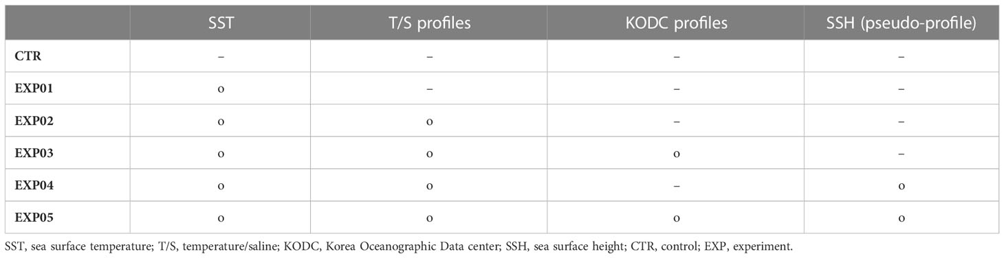
Table 1 Summary of the sensitivity experiment.

2.2.2 In-situ data

In-situ T/S profile data, which were obtained from various platforms, including conductivity temperature and depth (CTD) sensors, ocean station data (OSD), expendable bathythermographs (XBT), and moored buoys (MRB), were obtained from the World Ocean Database 2018 (WOD). The National Institute of Fisheries Science (NIFS) has produced a KODC database by researching the marine environment, including temperature, as well as other variables such as nutrient concentration and salinity, using CTD at standard observation depths (0, 10, 20, 30, 50, 75, 100, 125, 150, 200, 250, 300, 400, and 500 m), in the seas around the Korean Peninsula six times a year (for even months) from 1961 to the present. The temperature profiles obtained from the KODC were used in this study. KODC salinity data were not used in this study because they contained serious time-dependent bias errors as previously reported by Park (2021). Figure 2A shows the KODC and WOD temperature profile data used when assimilating the profile in February. We used 852 temperature data points collected from 23 stations. These in-situ profile data were assimilated into KOOS-OPEM every seven days.

FIGURE 2

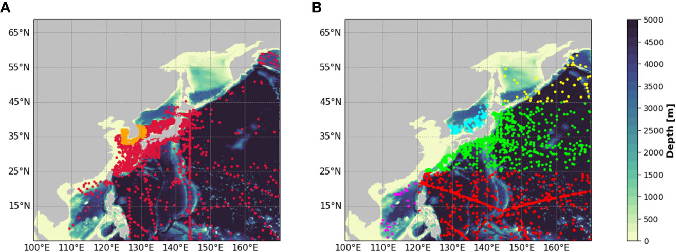
Figure 2 Distribution of in-situ temperature profiles used in data assimilation and validation. (A) temperature profiles used in data assimilation in February 1993. Crimson and orange dots denote profiles taken from World Ocean Database 2018 and Korea Oceanographic Data Center (KODC), respectively. (B) temperature profiles used in validation. Red, magenta, yellow, cyan and green dots denote temperature profiles located Northwestern Pacific (NWP), South China Sea (SCS), Oyashio Current (OYC), East/Japan Sea (EJS) and Kuroshio-Kuroshio Extension (K-KE) region, respectively.

To compare the performance of the vertical profiles of temperature and salinity, the independent T/S profiles (depth above approximately 500 m) of WOD and KODC, not used for assimilation, were used. When selecting the validation data, one-third of the total data was randomly selected. The spatial distribution of the validation profile is shown in Figure 2B.

2.2.3 Satellite data

The National Centers for Environmental Information (NOAA)’s 1/4° daily optimum SST (OISST) generated by interpolating and extrapolating observations from different platforms such as satellites, buoys, ships, and Argo floats were assimilated into KOOS-OPEM every day. The along-track SSH data from TOPEX/POSEIDON and ERS-1 were downloaded from CMEMS and used to construct the pseudo-profiles. The original resolution of the along-track SSH data was approximately 7 km; however, we used along-track data subsampled every 50 km to efficiently use computational resources. The pseudo-profiles derived from the along-track data were also assimilated daily.

To compare the performance of SST, the Operational Sea Surface Temperature and Sea Ice Analysis (OSTIA; Good et al., 2020) analysis downloaded from CMEMS was used. These data were generated from satellite and in-situ data through high-resolution analysis and intercomparison with spatial and temporal resolutions of 0.054° and daily, respectively. Gridded absolute dynamic topography data were used to compare the performance of the SSH. The temporal and spatial resolution of these data were one day and 1/4°, respectively. Because the gridded SSH data were generated by merging SSH measurements from multiple satellite altimetry, it can be suggested that the generated data are dependent on along-track data. However, as we did not directly assimilate the along-track data but assimilated pseudo-profiles instead, the results are independent of the gridded data.

2.2.4 Statistical metrics

The metrics used to assess assimilation performance were the root-mean-square error (RMSE) and impact of assimilation (IOA), as defined by Chen et al. (2018). These metrics are defined as follows:

$\begin{array}{ll}\text{RMSE=}\sqrt{\frac{1}{n}{\displaystyle {\sum }_{i=1}^n{(M_i-O_i)}^2}}& (8)\end{array}$

$\begin{array}{ll}\text{IOA=}\frac{RMS{E}_{CTR}-RMS{E}_{EXP}}{RMS{E}_{CTR}}\times 100& (9)\end{array}$

where M_i is the i^th model result of each experiment, O_i is the i^th observation, n is the number of values, and the overbar is the average over all periods. RMSE_CTR and RMSE_EXP denote the RMSEs of the CTR and assimilation experiment with respect to the observation, respectively. IOA is a metric that indicates the improvement of the RMSE compared to CTR. The larger the IOA, the greater the improvement in ocean analysis by the assimilation of each variable.

3 Results

3.1 Sea surface temperature

Figure 3 shows the comparison of the spatial distribution of the RMSE for SST with respect to OSTIA of all experiments. All experiments showed a large RMSE near the Korean and Chinese coastlines. The RMSE of the CTR was large in the middle and high-latitude regions, including the EJS and Kuroshio-Kuroshio Extension (K-KE), and was the largest in K-KE. The RMSEs of all assimilation experiments were greatly reduced in most regions by SST assimilation. In particular, the RMSEs of all experiments were significantly improved in the EJS and K-KE regions with a large RMSE in the CTR. However, the difference in the RMSE of SST is not significant in Figure 3 for the SST is constrained in all experiments by assimilating the OISST. The contributions of in-situ T/S profiles and SSH will be shown in next sections.

FIGURE 3

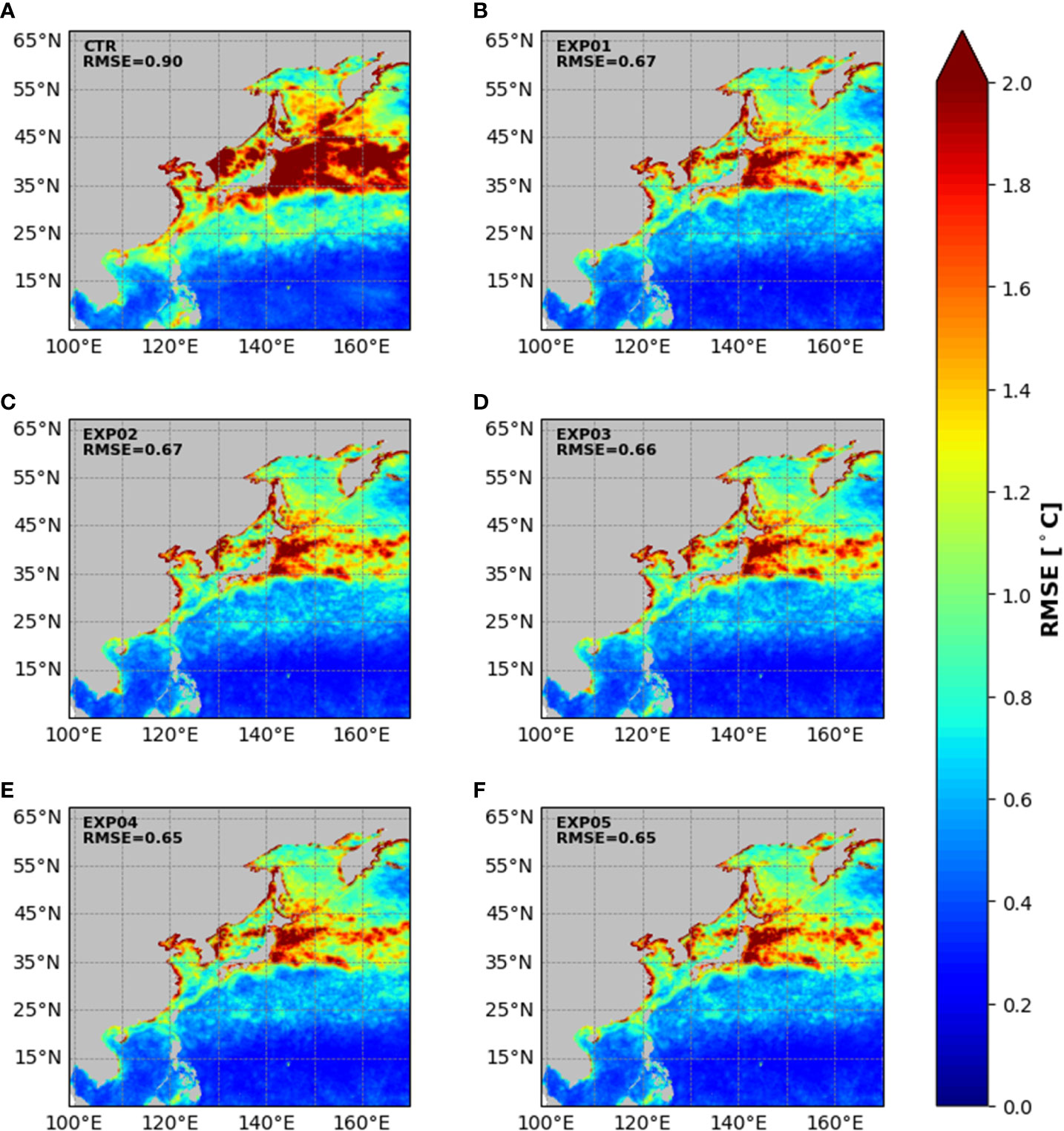
Figure 3 Spatial distribution of RMSE for SST with respect to OSTIA SST. Spatial averaged RMSEs of each experiment are shown on each figure. (A-F) represent the results of CTR and EXP01-05, respectively. RMSE, root-mean-square error; SST, sea salt temperature; CTR, control; EXP, experiment; OSTIA, Operational Sea Surface Temperature, and Sea Ice Analysis.

Table 2 compares the RMSE and IOA for SST by region for all assimilation experiments. The EXP01 of the average IOA was approximately 23.77%, and IOA was the highest in the K-KE region. In the NWP and OYC regions, the RMSE further improved after assimilating the T/S profiles. In the K-KE and EJS regions, the RMSE improved after assimilating the pseudo-profiles; however, in the OYC region, the RMSE increased. In the EJS region, EXP03 and EXP05, in which the profiles of KODC were assimilated, showed a higher IOA than EXP02 and EXP04, and EXP03 which did not assimilate the pseudo-profiles showed a lower RMSE than EXP04. These results indicate that the assimilation of SST satellite data plays a major role in improving the SST field, and that T/S and pseudo-profiles also play a partial role. However, the assimilation of the pseudo-profiles resulted in a slight increase in the RMSE at higher latitudes, such as the OYC region. Moreover, the KODC data reduced the RMSE for SST in the EJS; however, this effect was not observed in other regions.

TABLE 2

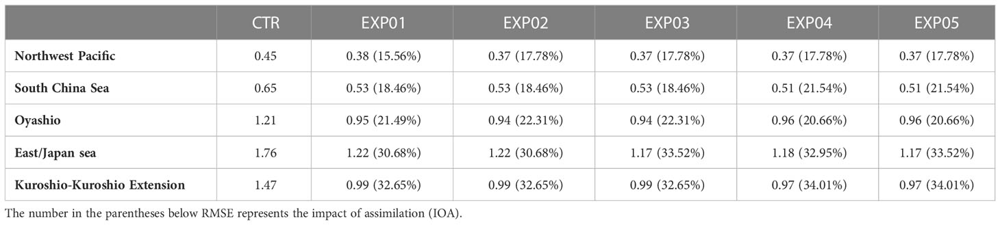
Table 2 Root-mean-square error (RMSE) averaged in space and time for SST by region from all experiments.

3.2 Vertical structure

The vertical performance of each experiment was evaluated using WOD18 and KODC data, which were not used for assimilation. To investigate regional effects, the domain was separated into five regions: NWP, SCS, OYC, EJS, and K-KE. Each region is denoted by a colored dot in Figure 2B.

Figure 4 shows the vertical profile of the RMSE for both temperature and salinity in each region. In the NWP region, the more observation data are assimilated, the lower the RMSE for the temperature and salinity at the overall depth. However, after assimilating SST, the RMSE for salinity in the subsurface layer increased compared to that of the CTR. Pseudo-profiles were the observational data that contributed the most to improving the RMSE for temperature and salinity in the NWP region. After the assimilation of these data, the RMSE for the temperature and salinity of the subsurface layer decreased substantially. Similar to the NWP region, in the SCS region, the pseudo-profiles contributed the most to reducing the RMSE, and assimilation of KODC data decreased the RMSE for temperature but increased that for salinity. In the OYC region, all experiments showed higher RMSE for temperature than that of the CTR at 50 m. However, in the subsurface layer, the RMSE decreased after assimilating the pseudo-profiles. The pseudo-profiles also contributed the most to reducing the RMSE in EJS and K-KE regions, and after assimilating KODC data, the RMSE for temperature decreased whereas that for salinity improved in both regions, although the salinity data of KODC were not assimilated. Tables 2 and 3 show the average RMSE of the profiles in Figure 4 by region. As mentioned above, because the RMSE of the other experiments was larger than that of the CTR at 50 m in the OYC, the average RMSE for the entire depth was larger than that of the CTR. These results indicate that pseudo-profiles derived from satellite altimetry data in most areas significantly contribute to improving the vertical structure of temperature and salinity, and the assimilation of KODC data improved the vertical structure of temperature and salinity in the K-KE and EJS regions. (Table 4)

FIGURE 4

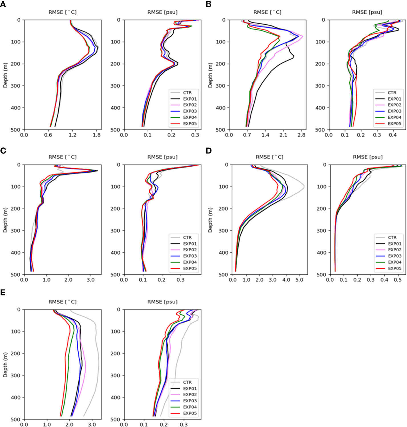
Figure 4 RMSE for temperature and salinity profiles at the region of (A) Northwestern Pacific (NWP), (B) South China Sea (SCS), (C) Oyashio Current (OYC), (D) East/Japan Sea (EJS), and (E) Kuroshio-Kuroshio extension (K-KE). Gray, black, violet, blue, green and red lines denote CTR and EXP01-05, respectively.

TABLE 3

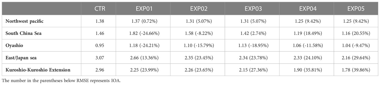
Table 3 RMSE averaged in space and time for temperature by region from all experiments.

TABLE 4

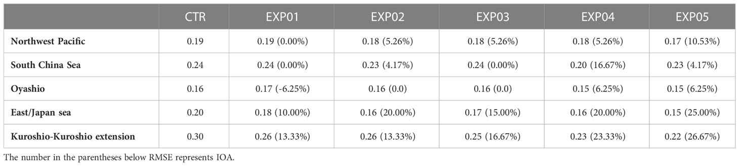
Table 4 RMSE averaged in space and time for salinity by region from all experiments.

To comprehensively evaluate the contribution of each observation data by region at the subsurface layer, IOA using the RMSE of the experiment according to the depth (100–500 m) with respect to the profile used for each independent validation was calculated and compared by averaging at intervals of 10° for the latitude and longitude.

Temperature (Figure 5), when only SST was assimilated (EXP01), had a negative effect on the subsurface layer of most regions, except for some regions in high-latitude regions. EXP02 and EXP03 that assimilated T/S profiles had improved RMSE over EXP01 in the NWP and SCS regions. The assimilation of pseudo-profiles (EXP04 and EXP05) significantly improved the RMSE in most areas, especially in the NWP and regions where the Kuroshio Current passes (120°E–140°E, 25°N–35°N). However, it did not have a significant effect in high-latitude regions (140°E–170°E, 35°N–65°N), except for the EJS. The assimilation of KODC data (EXP03 and EXP05) considerably improved the RMSE not only in the EJS but also in the region where Kuroshio passes and the K-KE region.

FIGURE 5

Figure 5 Distribution of mean IOA for temperature at subsurface layer. (A-E) represent the results of EXP01-05, respectively.

In addition, by comparing the IOA for salinity in each experiment (Figure 6), we found that the assimilation of SST did not improve the RMSE for salinity in the subsurface layer in most regions. The assimilation of the T/S profile substantially improved the RMSE in the NWP and SCS regions, and the assimilation of the pseudo-profiles or the temperature substantially improved the RMSE in the regions where the Kuroshio Current passed; however, the effect of the assimilation of the temperature was not substantial in high-latitude regions. In the assimilation of KODC (EXP03 and EXP05), the RMSE of EXP05, which also assimilated pseudo-profiles, improved in both the EJS and K-KE regions. These results show that the assimilation of SST did not have a significant impact on the subsurface layer whereas that of T/S profiles improved the RMSE in most regions. In addition, the assimilation of pseudo-profiles played a significant role in improving the temperature and salinity at the subsurface layer, similar to the in-situ T/S profile data; however, it did not show a significant contribution in high-latitude regions. The assimilation of KODC data, which is Korean marginal sea data, improved the temperature at the subsurface layer in the K-KE and EJS regions, and salinity at the subsurface layer was improved when assimilated with pseudo-profiles.

FIGURE 6

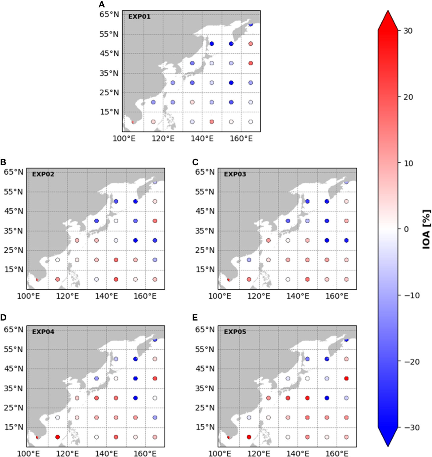
Figure 6 Distribution of mean IOA for salinity at subsurface layer. (A-E) represent the results of EXP01-05, respectively.

3.3 Sea surface height

Figure 7 shows the time series of monthly spatial-averaged RMSE for SSH from all experiments according to each region. Pseudo-profiles and SST contributed the most to improving the RMSE for SSH in all regions. SST also improved the RMSE for SSH in all regions. The T/S profiles improved the RMSE for SSH regardless of the season in the NWP region; however, it did not significantly improve the RMSE for SSH in the OYC regions and increased it during the summer season in the K-KE and EJS regions. Moreover, the RMSE of EXP03, which assimilated KODC data, increased from August to November compared to that of EXP02. Notably, the RMSE of EXP05 which assimilated KODC and pseudo-profiles improved from May to September compared to that of EXP04 which did not assimilate KODC data. The data assimilation of KODC data appeared to be more effective in EXP05 with SSH assimilation that in EXP03 without SSH assimilation. The RMSE of EXP05, which assimilated pseudo-profiles, was improved in the NWP during the summer and in the K-KE region from April to June and September to October.

FIGURE 7

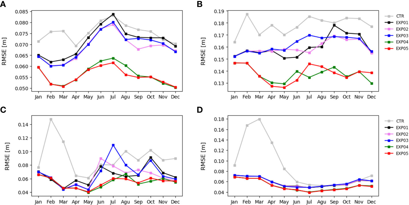
Figure 7 Monthly mean RMSE for sea surface height at the region of (A) Northwestern Pacific (NWP), (B) Kuroshio-Kuroshio extension (K-KE), (C) East/Japan Sea (EJS) and (D) Oyashio Current (OYC). Gray, black, violet, blue, green and red lines denote CTR and EXP01-05, respectively.

To evaluate the oceanic variability associated with the K-KE region, the Kuroshio axis of the AVISO gridded data and that of each experiment were compared (Figure 8). In January and February, the assimilation effect of each experiment did not appear significant; however, the assimilation effect of each experiment became evident over time, starting in March. The experiments that did not assimilate the pseudo-profiles, including CTR, excessively simulated mesoscale features, such as meandering and eddies. However, experiments that assimilated the pseudo-profiles constrained the features excessively simulated in other experiments. EXP05, which assimilated KODC data, better simulated the Kuroshio axis in most months, except for July and August, compared to EXP04.

FIGURE 8

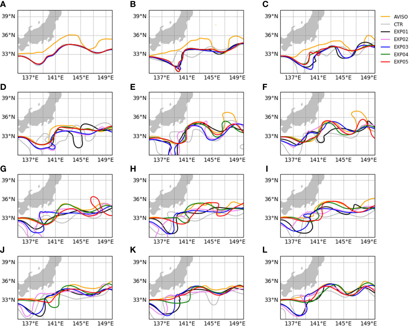
Figure 8 Monthly mean Kuroshio axis is denoted by the 0.6m SSH. A–L represent results in January-December, respectively. Orange line denotes Kuroshio axis from the AVISO gridded data. Gray, black, violet, blue, green and red lines denote Kuroshio axis of CTR and EXP01-05, respectively.

To evaluate this result more quantitatively, the RMSE for the latitude of the Kuroshio axis with respect to the observational data of each experiment was calculated and compared (Figure 9). The observation data that contributed the most to improving the Kuroshio axis were the pseudo-profiles derived from satellite altimetry data except in January and February. The system seems to become unstable in the beginning as the psudo-profiles from satellite altimetry have been newly assimilated. However, from March, EXP04 and EXP05 show better representation of the Kuroshio axis rather than other experiments. The SST data also contributed to improving the Kuroshio axis to some extent whereas the T/S profiles did not show a significant impact. EXP05, which assimilated all observations presented in this study, including KODC, reduced the RMSE for the latitude of the Kuroshio axis, except for March and the summer season, compared to EXP04, which assimilated all observations except KODC. Table 5 also confirms the contribution of the satellite altimetry and KODC profile data to the significant reduction in RMSE for latitude of the Kuroshio axis. These results suggest that regional ocean observation networks may improve the forecast skill of the ocean prediction system not only in the region but also in the open ocean, such as the Pacific Ocean.

FIGURE 9

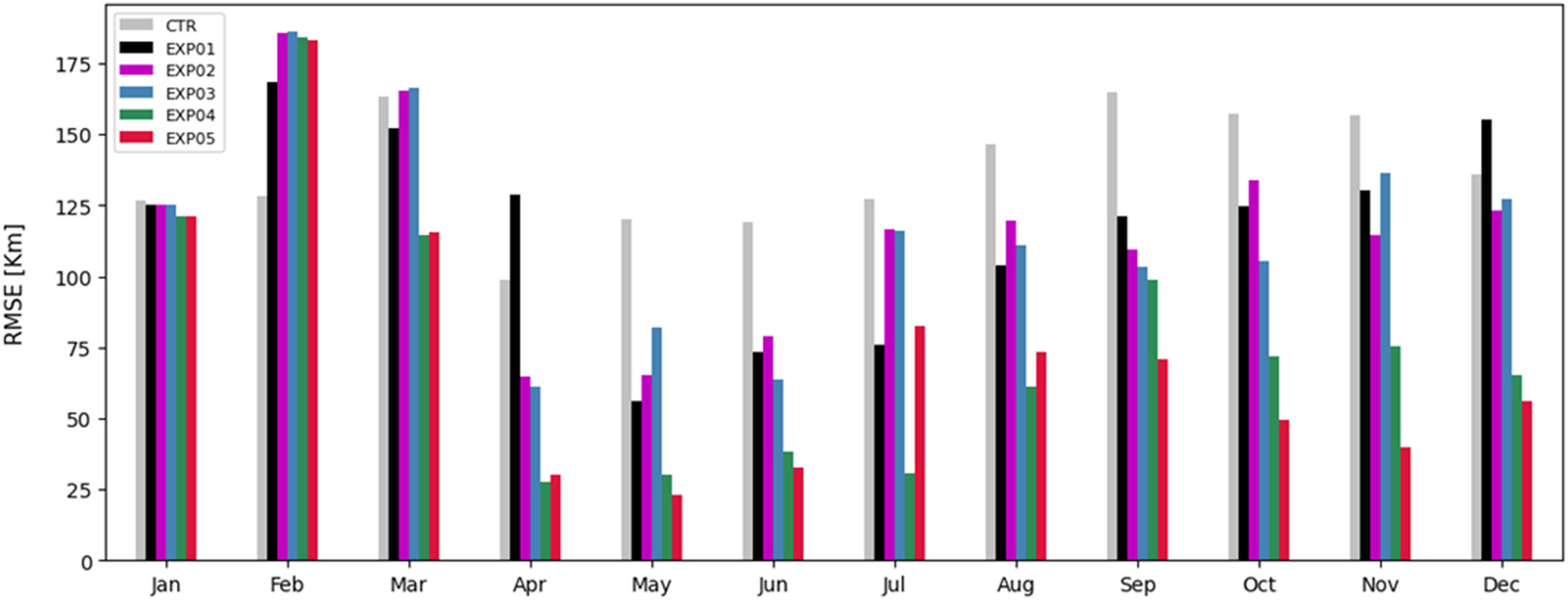
Figure 9 Monthly mean RMSEs for the latitude of the Kuroshio axis with respect to the observation data of each experiment. Gray, black, violet, blue, green and red bars denote CTR and EXP01-05, respectively.

TABLE 5

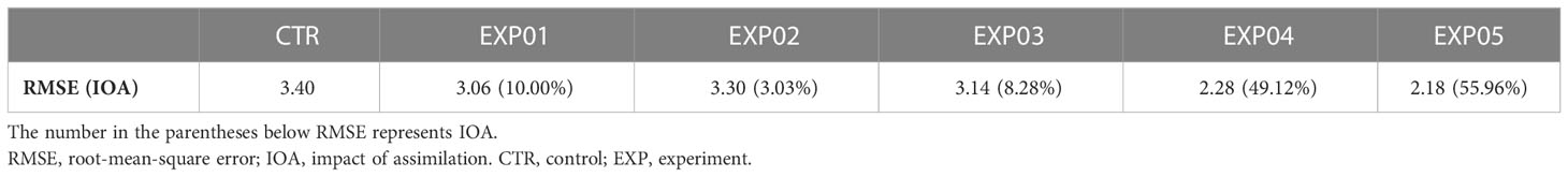
Table 5 RMSE averaged in space and time for the latitude of the Kuroshio axis with respect to AVISO gridded data in each experiment.

4 Discussion

In this study, sensitivity experiments were conducted to evaluate the impacts of in-situ T/S profiles and satellite observation data, including SST and altimetry data, on a high-resolution ocean circulation prediction system, so called the KOOS-OPEM. KOOS-OPEM adopts localized EnOI to assimilate the ocean observation data into the model. The satellite altimetry information was projected into the subsurface layer following CH96 which did not directly assimilate the altimetry but rather pseudo temperature and salinity profiles. The contribution of each observation data was evaluated as follows: IOA of EXP01 for SST data; average of IOA differences of EXP02 and EXP03 with respect to EXP01 for in-situ T/S profile data; average of IOA differences between EXP02 and EXP03, and between EXP04 and EXP05 for KODC data; average of IOA differences between EXP02 and EXP04, and between EXP03 and EXP05 for altimetry data.

The comparisons of model experiments suggest that the satellite SST data set has the most contribution (EXP01, 23.77%) to the modeled SST improvement in terms of the RMSE compared to the CTR. Especially, the largest improvement was found in the K-KE region (32.65%). Additionally, assimilating the in-situ profiles insignificant impact on the modeled SST performance (EXP02), while the in-situ profiles have the greatest influence on the vertical structure of temperature (average 10.26%) and salinity (average 7.50%), especially in the EJS (EXP02 and EXP03). The altimetry assimilation (EXP04 and EXP05) also contributes to improving the subsurface vertical profile structure of ocean temperature (average 12.33%) and salinity (average 10.00%), especially in the K-KE region. It is highlighted that the in-situ profiles in the Korean marginal seas provided by KODC have significant impact on the vertical structure of ocean temperature and salinity in not only the EJS but also the K-KE region (EXP03 and EXP05).

The assimilation of SST had a negative effect on both temperature and salinity in the subsurface layer in most areas (Figures 5, 6). In the OYC region, moreover, the SST assimilation seems to increase the RMSE of the temperature around 50 m depth, where the background error variance has a maximum (not shown here). Indeed, it has been observed that the model overestimates the variability of the temperature more than the observation around 50 m depth in the OYC region. The background error covariance calculated from the historical simulation may induce the temperature degradation in this region. In addition, the number of in-situ T/S profiles is not sufficient and the contribution of SSH seems to be limited in this region. To resolve the temperature degradation in the OYC region, it is necessary to add a new dataset or improve the model performance, which is left for the next study.

In-situ T/S profile data assimilation was effective in most regions, and pseudo-profile data also substantially contributed to improving both temperature and salinity vertical structures as effectively as the in-situ T/S profile data. However, the contribution of pseudo-profiles at high latitudes was lower than at low- and middle-latitudes. In high latitude oceans, where stratification is weak, small changes in surface height are assimilated into large vertical displacements of the water column, which can rather lead to errors (Fox et al., 2000). Therefore, when using the altimetry assimilation method based on CH96, it is necessary to introduce latitude dependency (Vidard et al., 2009) for the next version. As mentioned above, KODC data improved the temperature in the subsurface layer not only in the East Sea but also in the K-KE region; when assimilation was performed using KODC data and pseudo-profiles, the salinity of the subsurface layer improved. Moreover, the assimilation of KODC data affected a large area (from 120°E to 160°E and 35°N to 45°N). Each observation also contributed to the improvement in the Kuroshio axis. When compared qualitatively, the pseudo-profiles derived from satellite altimetry data constrained mesoscale features, such as meander and eddy that were excessively simulated. When compared quantitatively (Table 5), the pseudo-profiles were the main contributors to the reduction in the RMSE for the latitude of the Kuroshio axis with respect to the AVISO gridded data by an average of 46.89%. SST satellite data also made the second largest contribution, improving the Kuroshio axis by 10.00%. The KODC data also improved the Kuroshio axis by 6.84% when assimilated with the pseudo-profiles.

This study suggests the quantitative impacts of each observation data sets for improvement of the high-resolution ocean prediction system. Notably, pseudo-profiles derived from satellite altimetry data significantly contributed to the ocean analysis field by improving the vertical structure of temperature and salinity. Especially, we clearly showed that the assimilation of the regional ocean observation provided by the Korean regional observation network has non-negligible impacts on the upper layer structure in the open ocean and the representation of the Kuroshio axis. These results highlight the role of regional ocean observation networks in ocean prediction systems to improve the analysis and forecast skills in the open ocean as well as in the region. In particular, it is interesting that data assimilation of the KODC data obtained around Korea peninsula contributes to the improvement of representation of the Kuroshio axis. Figures 10A-D show the upper ocean structures of temperature and current speed between EXP04 and EXP05, respectively, in October. It is noteworthy that the differences in temperature and current between EXP04 and EXP05 was pronounced in the EJS, east of the Tsugaru strait and Kuroshio downstream region rather than in the Kuroshio upstream region. In EXP05, compared to EXP04, the warm water from the Tsugaru Strait extended to the east, and the cold water from the Okhotsk Sea and the Subarctic Pacific was extended to the south. Itoh et al. (2022) analyzed high-resolution observation data and reported that a sharp front often develops in the Sanriku confluence where Tsugaru Warm Current, Oyasio Current, and Kuroshio Current meet. EXP05 may better simulate the representation of the front in the Sanriku confluence by improving the physical properties of the Tsugaru Warm current through the assimilation of KODC data taken around Korean Peninsula. In addition, the better representation of the front may help the Oyashio Current extend to the south where the Kuroshio Current separate from the coast, which affects the fluctuations of the Kuroshio axis. In fact, the IOA from the temperature profiles for EXP04 and EXP05 (Figures 10E, F) shows that the KODC profiles contribute to improving the vertical temperature structure not only around the Korean Peninsula but also in the west of the Tsugaru strait and in the Sanriku confluence. Although the dynamic relationship between the circulation of the Korea marginal seas and Kuroshio was not fully understood in this study, it seems worthwhile for future research. This study also suggests that greater attention should be paid to the role of regional ocean observation networks to improve the forecast skill of the ocean prediction system not only in the region but also in the open ocean, such as the Pacific Ocean.

FIGURE 10

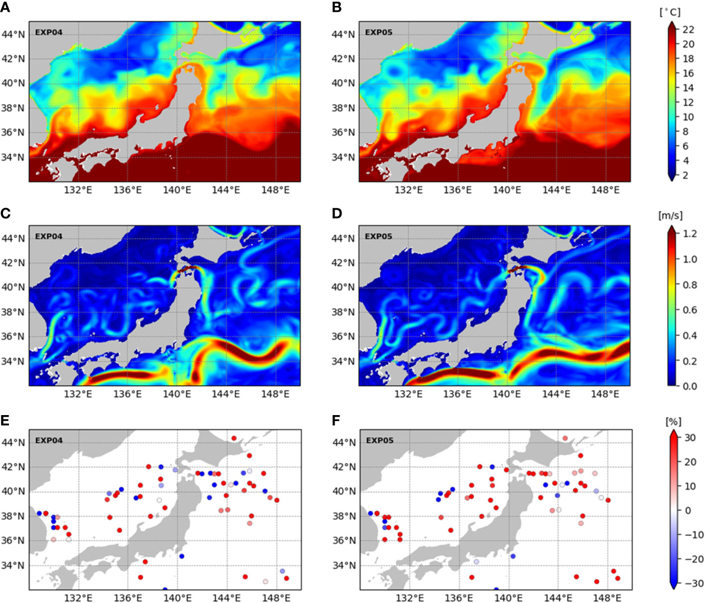
Figure 10 Monthly mean temperature (upper panels), current speed (middle panels) averaged over 0 to 100m, and IOA (lower panels) for the temperature profiles over 0 to 100m in EXP04 (left panels) and EXP05 (right panels) in October.

Data availability statement

The original contributions presented in the study are included in the article/supplementary material, Further inquiries can be directed to the corresponding author.

Author contributions

IC and YK: conducting the experiment and writing the first manuscript. IC: carrying out experiment and visualization. YK: supervision. YK, HJ and GP: deriving additional analysis ideas. YK, HJ, GP, Y-GP and Y-SC: review and editing. All authors contributed to the article and approved the submitted version.

Funding

This research was part of projects titled ‘Investigation and prediction system development of marine heatwave around the Korean Peninsula originated from the subarctic and western Pacific’ (20190344) and ‘Improvements of ocean prediction accuracy using numerical modeling and artificial intelligence technology’ (20180447) funded by the Ministry of Oceans and Fisheries, Korea. This work was supported by Korea Institute of Marine Science and Technology Promotion(KIMST) funded by the Ministry of Oceans and Fisheries, Korea (Development of 3-D Ocean Current Observation Technology for Efficient Response to Maritime Distress, 20210642). YK was supported by by the Pukyong National University Research Fund (CD20191541).

Acknowledgments

We would like to thank Gary Brassington for his valuable discussions and comments.

Conflict of interest

The authors declare that the research was conducted in the absence of any commercial or financial relationships that could be construed as a potential conflict of interest.

Publisher’s note

All claims expressed in this article are solely those of the authors and do not necessarily represent those of their affiliated organizations, or those of the publisher, the editors and the reviewers. Any product that may be evaluated in this article, or claim that may be made by its manufacturer, is not guaranteed or endorsed by the publisher.

References

Alves J. O. S., Haines K., Anderson D. L. (2001). Sea Level assimilation experiments in the tropical pacific. J. Phys. Oceanogr. 31 (2), 305–323. doi: 10.1175/1520-0485(2001)031<0305

CrossRef Full Text | Google Scholar

Arakawa A., Lamb V. R. (1977). Computational design of the basic dynamical processes of the UCLA general circulation model. Gen. Circ. Models atmosphere 17 (Supplement C), 173–265. doi: 10.1016/B978-0-12-460817-7.50009-4

CrossRef Full Text | Google Scholar

Birol F., Brankart J. M., Lemoine J. M., Brasseur P., Verron J. (2005). Assimilation of satellite altimetry referenced to the new GRACE geoid estimate. Geophys. Res. Lett. 32 (6). doi: 10.1029/2004GL021329

CrossRef Full Text | Google Scholar

Burgers G., Van Leeuwen P. J., Evensen G. (1998). Analysis scheme in the ensemble kalman filter. Monthly weather Rev. 126 (6), 1719–1724. doi: 10.1175/1520-0493(1998)126<1719:ASITEK>2.0.CO;2

CrossRef Full Text | Google Scholar

Chen Y., Yan C., Zhu J. (2018). Assimilation of sea surface temperature in a global hybrid coordinate ocean model. Adv. Atmospheric Sci. 35 (10), 1291–1304. doi: 10.1007/s00376-018-7284-6

CrossRef Full Text | Google Scholar

Cho Y. K., Seo G. H., Choi B. J., Kim S., Kim Y. G., Youn Y. H., et al. (2009). Connectivity among straits of the northwest pacific marginal seas. J. Geophys. Res.: Oceans 114 (C6). doi: 10.1029/2008JC005218

CrossRef Full Text | Google Scholar

Cooper M., Haines K. (1996). Altimetric assimilation with water property conservation. J. Geophys. Res.: Oceans 101 (C1), 1059–1077. doi: 10.1029/95JC02902

CrossRef Full Text | Google Scholar

Counillon F., Bertino L. (2009). Ensemble optimal interpolation: multivariate properties in the gulf of Mexico. Tellus A: Dynam. Meteorol. Oceanogr. 61 (2), 296–308. doi: 10.1111/j.1600-0870.2008.00383.x

CrossRef Full Text | Google Scholar

El-Geziry T. M., Bryden I. G. (2010). The circulation pattern in the Mediterranean Sea: issues for modeller consideration. J. Operational Oceanogr. 3 (2), 39–46. doi: 10.1080/1755876X.2010.11020116

CrossRef Full Text | Google Scholar

Evensen G. (1994). Sequential data assimilation with a nonlinear quasi-geostrophic model using Monte Carlo methods to forecast error statistics. J. Geophys. Res.: Oceans 99 (C5), 10143–10162. doi: 10.1029/94JC00572

CrossRef Full Text | Google Scholar

Evensen G. (2003). The ensemble kalman filter: Theoretical formulation and practical implementation. Ocean dynam. 53 (4), 343–367. doi: 10.1007/s10236-003-0036-9

CrossRef Full Text | Google Scholar

Fox A. D., Haines K., De Cuevas B., Webb D. J. (2000). Altimeter assimilation in the OCCAM global model: Part I: A twin experiment. J. Mar. Syst. 26 (3-4), 303–322. doi: 10.1016/S0924-7963(00)00043-9

CrossRef Full Text | Google Scholar

Fu W., Zhu J. (2011). Effects of sea level data assimilation by ensemble optimal interpolation and 3D variational data assimilation on the simulation of variability in a tropical pacific model. J. Atmospheric Oceanic Technol. 28 (12), 1624–1640. doi: 10.1175/JTECH-D-11-00044.1

CrossRef Full Text | Google Scholar

Gaspari G., Cohn S. E. (1999). Construction of correlation functions in two and three dimensions. Q. J. R. Meteorol. Soc. 125 (554), 723–757. doi: 10.1002/qj.49712555417

CrossRef Full Text | Google Scholar

Gent P. R., Mcwilliams J. C. (1990). Isopycnal mixing in ocean circulation models. J. Phys. Oceanogr. 20 (1), 150–155. doi: 10.1175/1520-0485(1990)020<0150

CrossRef Full Text | Google Scholar

Good S., Fiedler E., Mao C., Martin M. J., Maycock A., Reid R., et al. (2020). The current configuration of the OSTIA system for operational production of foundation sea surface temperature and ice concentration analyses. Remote Sens. 12 (4), 720. doi: 10.3390/rs12040720

CrossRef Full Text | Google Scholar

Griffies S. M., Hallberg R. W. (2000). Biharmonic friction with a smagorinsky-like viscosity for use in large-scale eddy-permitting ocean models. Monthly Weather Rev. 128 (8), 2935–2946. doi: 10.1175/1520-0493(2000)128<2935

CrossRef Full Text | Google Scholar

Hamill T. M., Whitaker J. S., Snyder C. (2001). Distance-dependent filtering of background error covariance estimates in an ensemble kalman filter. Monthly Weather Rev. 129 (11), 2776–2790. doi: 10.1175/1520-0493(2001)129<2776

CrossRef Full Text | Google Scholar

Houtekamer P. L., Mitchell H. L. (2001). A sequential ensemble kalman filter for atmospheric data assimilation. Monthly Weather Rev. 129 (1), 123–137. doi: 10.1175/1520-0493(2001)129<0123

CrossRef Full Text | Google Scholar

Itoh S., Tsutsumi E., Masunaga E., Sakamoto T. T., Ishikawa K., Yanagimoto D., et al. (2022). Seasonal cycle of the confluence of the tsugaru warm, oyashio, and kuroshio currents east of Japan. J. Geophys. Res.: Oceans 127 (8), e2022JC018556. doi: 10.1029/2022JC018556

CrossRef Full Text | Google Scholar

Kim Y. H., Hwang C., Choi B. J. (2015). An assessment of ocean climate reanalysis by the data assimilation system of KIOST from 1947 to 2012. Ocean Model. 91, 1–22. doi: 10.1016/j.ocemod.2015.02.006

CrossRef Full Text | Google Scholar

Kim Y. H., Lyu S. J., Choi B. J., Cho Y. K., Kim Y. G. (2008). Implementation of the ensemble kalman filter to a double gyre ocean and sensitivity test using twin experiments. Ocean Polar Res. 30 (2), 129–140. doi: 10.4217/OPR.2008.30.2.129

CrossRef Full Text | Google Scholar

Kim S. Y., Park Y. G., Kim Y. H., Seo S., Jin H., Pak G., et al. (2021). Origin, variability, and pathways of East Sea intermediate water in a high-resolution ocean reanalysis. J. Geophys. Res.: Oceans 126 (6), e2020JC017158. doi: 10.1029/2020JC017158

CrossRef Full Text | Google Scholar

Large W. G., McWilliams J. C., Doney S. C. (1994). Oceanic vertical mixing: A review and a model with a nonlocal boundary layer parameterization. Rev. geophysics 32 (4), 363–403. doi: 10.1029/94RG01872

CrossRef Full Text | Google Scholar

Large W. G., Yeager S. G. (2004). Diurnal to decadal global forcing for ocean and sea-ice models: The data sets and flux climatologies. NCAR Tech. Rep. TN-460+STR, 105–129. doi: 10.5065/D6KK98Q6

CrossRef Full Text | Google Scholar

Oke P. R., Brassington G. B., Griffin D. A., Schiller A. (2008). The bluelink ocean data assimilation system (BODAS). Ocean Model. 21 (1-2), 46–70. doi: 10.1016/j.ocemod.2007.11.002

CrossRef Full Text | Google Scholar

Oke P. R., Sakov P., Corney S. P. (2007). Impacts of localisation in the EnKF and EnOI: experiments with a small model. Ocean Dynam. 57 (1), 32–45. doi: 10.1007/s10236-006-0088-8

CrossRef Full Text | Google Scholar

Oke P. R., Schiller A., Griffin D. A., Brassington G. B. (2005). Ensemble data assimilation for an eddy-resolving ocean model of the Australian region. Q. J. R. Meteorol. Soc. 131 (613), 3301–3311. doi: 10.1256/qj.05.95

CrossRef Full Text | Google Scholar

Parent L., Testut C. E., Brankart J. M., Verron J., Brasseur P., Gourdeau L. (2003). Comparative assimilation of Topex/Poseidon and ERS altimeter data and of TAO temperature data in the tropical pacific ocean during 1994–1998, and the mean sea-surface height issue. J. Mar. Syst. 40, 381–401. doi: 10.1016/S0924-7963(03)00026-5

CrossRef Full Text | Google Scholar

Park J. (2021). Quality evaluation of long-term shipboard salinity data obtained by NIFS. Sea: J. OF THE KOREAN Soc. OF OCEANOGR. 26 (1), 49–61. doi: 10.7850/jkso.2021.26.1.049

CrossRef Full Text | Google Scholar

Park Y. G., Choi A., Kim Y. H., Min H. S., Hwang J. H., Choi S. H. (2010). Direct flows from the ulleung basin into the yamato basin in the East/Japan Sea. Deep Sea Res. Part I: Oceanographic Res. Papers 57 (5), 731–738. doi: 10.1016/j.dsr.2010.03.006

CrossRef Full Text | Google Scholar

Park K., Park J. E., Choi B. J., Byun D. S., Lee E. I. (2013). An oceanic current map of the East Sea for science textbooks based on scientific knowledge acquired from oceanic measurements. Sea: J. Korean Soc. Oceanogr. 18 (4), 234–265. doi: 10.7850/jkso.2013.18.4.234

CrossRef Full Text | Google Scholar

Seo S. N. (2008). Digital 30sec gridded bathymetric data of Korea marginal seas-KorBathy30s. J. Korean Soc. Coast. Ocean Engineers 20 (1), 110–120.

Google Scholar

Simmons H. L., Jayne S. R., Laurent L. C. S., Weaver A. J. (2004). Tidally driven mixing in a numerical model of the ocean general circulation. Ocean Model. 6 (3-4), 245–263. doi: 10.1016/S1463-5003(03)00011-8

CrossRef Full Text | Google Scholar

Testut C. E., Brasseur P., Brankart J. M., Verron J. (2003). Assimilation of sea-surface temperature and altimetric observations during 1992–1993 into an eddy permitting primitive equation model of the north Atlantic ocean. J. Mar. Syst. 40, 291–316. doi: 10.1016/S0924-7963(03)00022-8

CrossRef Full Text | Google Scholar

Troccoli A., Balmaseda M. A., Segschneider J., Vialard J., Anderson D. L., Haines K., et al. (2002). Salinity adjustments in the presence of temperature data assimilation. Monthly Weather Rev. 130 (1), 89–102. doi: 10.1175/1520-0493(2002)130<0089

CrossRef Full Text | Google Scholar

Troccoli A., Haines K. (1999). Use of the temperature–salinity relation in a data assimilation context. J. Atmospheric Oceanic Technol. 16 (12), 2011–2025. doi: 10.1175/1520-0426(1999)016<2011

CrossRef Full Text | Google Scholar

Troen I. B., Mahrt L. (1986). A simple model of the atmospheric boundary layer; sensitivity to surface evaporation. Boundary-Layer Meteorol. 37 (1), 129–148. doi: 10.1007/BF00122760

CrossRef Full Text | Google Scholar

Vialard J., Weaver A. T., Anderson D. L. T., Delecluse P. (2003). Three-and four-dimensional variational assimilation with a general circulation model of the tropical pacific ocean. part II: Physical validation. Monthly Weather Rev. 131 (7), 1379–1395. doi: 10.1175/1520-0493(2003)131<1379

CrossRef Full Text | Google Scholar

Vidard A., Balmaseda M., Anderson D. (2009). Assimilation of altimeter data in the ECMWF ocean analysis system 3. Monthly Weather Rev. 137 (4), 1393–1408. doi: 10.1175/2008MWR2668.1

CrossRef Full Text | Google Scholar

Vörösmarty C. J., Fekete B., Tucker. B. A. (1998). River discharge database, version 1.1 (RivDIS v1.0 supplement) [Available online at http://pyramid.sr.unh.edu/csrc/hydro/.]. doi: 10.1594/PANGAEA.859439

CrossRef Full Text | Google Scholar

Winton M. (2000). A reformulated three-layer sea ice model. J. atmospheric oceanic Technol. 17 (4), 525–531. doi: 10.1175/1520-0426(2000)017<0525

CrossRef Full Text | Google Scholar

Yan C., Zhu J., Li R., Zhou G. (2004). Roles of vertical correlations of background error and T-s relations in estimation of temperature and salinity profiles from sea surface dynamic height. J. Geophys. Res.: Oceans 109 (C8). doi: 10.1029/2003JC002224

CrossRef Full Text | Google Scholar

Zheng F., Zhu J. (2015). Roles of initial ocean surface and subsurface states on successfully predicting 2006–2007 El niño with an intermediate coupled model. Ocean Sci. 11 (1), 187–194. doi: 10.5194/os-11-187-2015

CrossRef Full Text | Google Scholar

Zhou W., Li J., Xu F., Shu Y., Feng Y. (2021). The impact of ocean data assimilation on seasonal predictions based on the national climate center climate system model. Acta Oceanol. Sin. 40 (5), 58–70. doi: 10.1007/s13131-021-1732-3

CrossRef Full Text | Google Scholar