Gravity disturbance compensation for dual-axis rotary modulation inertial navigation system

1 Introduction

Inertial navigation systems (INS) are widely employed to establish autonomous navigation systems in various fields. This auto-navigation feature renders INS stable and reliable for any type of external interference. However, INS is hindered by errors caused by inertial devices, which severely restrict the underwater long-time navigation ability of the submersible. With the development and application of optical inertial devices and rotary modulation technologies, the accuracy of inertial sensors has significantly improved (Wen et al., 2009; Yuan et al., 2012; Zhou et al., 2018; Wu and Li, 2019). However, some errors have been overlooked and have become the key restricting factors to further improvements in the positioning accuracy of INS, such as horizontal gravity disturbances. In fact, systematic errors caused by gravity disturbances have gradually become one of the main errors. Accurate gravity compensation for INS is an effective means of promoting the long-endurance positioning capability of underwater vehicles (Kwon and Jekeli, 2005; Jekeli et al., 2007; Zhou et al., 2016; Tie et al., 2018; Wen et al., 2020).

Gravity compensation is an important part of gravity-aided navigation for INS. Some scholars have studied the influence of gravity disturbances on INS. Gelb and Levine (1969) modeled gravity disturbance as a Gaussian Markov process and quantitatively evaluated its impact of gravity disturbance on the INS. Jordan (1973) established a Markov model based on variance analysis and analyzed the impact of horizontal gravity disturbances on the INS. These stochastic model methods can be used to estimate gravity disturbance. However, the Earth gravity field (gravity disturbance and gravity anomaly) is inhomogeneous and complex, and a single stochastic model cannot represent the variation in the gravity field. Second, a large amount of prior information must be provided to accurately estimate the stochastic model parameters. Therefore, achieving gravity compensation for an INS based on a stochastic model is not an optimal approach. The second gravity compensation method is a real-time compensation method that uses a gravity gradiometer. The development of the gravity gradiometer made it possible to derive the gravity vector, allowing the mechanical arrangement of the INS to be improved by providing the gravity vector measured using the gravity gradiometer to the INS. Jekeli (2006) proposed an INS gravity compensation method based on a gravity gradiometer that could correct the inertial navigation error through full tensor gravity gradient measurements. However, the use of gravity compensation methods based on gravity gradiometers is hindered by their high cost (Heller and Jordan, 2015). In recent decades, a high-degree Earth gravity field model (GFM) has been developed that can be used to achieve gravity disturbance compensation for INS. Wang et al. (2016) studied gravity compensation based on the EGM2008 gravity model and focused on the impact of the truncation degree/order of the GFM for gravity compensation. Similarly, Chang et al. (2019) utilized a high-degree EIGEN_6C4 model for gravity compensation.

The mechanical arrangement of the INS can be improved by measuring the gravity disturbance determined by high-degree GFMs, such as EGM2008 and EIGEN_6C4 (Pavlis et al., 2012; Förste et al., 2014), with the maximum degree of these GFMs being only 2190 (~10 km). For high-frequency gravity field signals with a spatial resolution less than ~10 km, these high-degree gravity field models still cannot be effectively represented and have certain omission errors owing to the lack of short-wavelength information. Tscherning and Rapp’s variance model showed that the gravity field models for degree 2190 have a gravity signal loss of gravity anomaly of 11.1 mGal and deflection of the vertical (DOV) of 1.7” (Tscherning and Rapp, 1974; Denker, 2013). Signal loss was more severe in the rugged terrain area. However, owing to the limited degree of high-degree GFMs, gravity compensation for INS based on GFMs cannot effectively represent high-frequency gravity field signals, which leads to accuracy loss of gravity compensation. In addition, there is a coupling effect between gravity disturbance and accelerometer drift bias (Hanson, 1988). It is still difficult to achieve gravity compensation by considering this coupling effect. From the aforementioned analysis, we can see that the gravity compensation of the INS is mainly related to two factors: (1) the accuracy and resolution of the horizontal gravity disturbance, and (2) the coupling effect between the accelerometer drift bias and gravity disturbance. Therefore, it is important to refine the gravity compensation background field and consider the coupling effect between accelerometer drift bias and gravity disturbance to achieve higher-accuracy gravity compensation.

With the continuous development of satellite altimetry missions, satellite altimetry has become the primary method for determining the global marine gravity field. The marine gravity anomaly and DOV with 1’ × 1’ (~2 km) resolution can be retrieved by integrating multigeneration altimetry satellites (Andersen et al., 2010; Bao et al., 2013; Sandwell and Smith, 2014; Sandwell et al., 2014; Sandwell et al., 2021). The high-resolution and high-precision marine gravity compensation background field can be determined by satellite altimetry, which provides a new way to achieve gravity compensation for INS. In addition, with the development of rotary modulation technologies, the accuracy of inertial sensors has significantly improved. Rotation modulation technology (RMT) can eliminate the accelerometer drift error by periodically rotating the inertial sensor along the rotation axis. Rotation modulation INS uses periodic dynamic motion to estimate the static error of inertial sensors. Inertial measuring unit (IMU) rotates regularly around the axis to modulate the static error into periodic signal to offset the impact of static error and improve the long-term navigation accuracy of inertial navigation. Owing to the introduction of the modulation mechanism, the accelerometer drift bias can be compensated and the coupling effect can be ignored in gravity compensation. Therefore, this study focuses on gravity compensation for dual-axis rotary modulation INS and aims to improve the positioning accuracy of the dual-axis rotary modulation INS. Herein, the error and frequency characteristics caused by gravity disturbance are analyzed, and the effect of gravity disturbance on the initial alignment is also investigated. A high-precision and high-resolution satellite altimetry marine gravity field model is used to compensate for the error caused by gravity disturbance, which can effectively represent the high-frequency gravity field signal. The horizontal gravity disturbance determined by the satellite altimetry model is provided to the dual-axis rotary modulation INS to achieve gravity compensation in the initial alignment and pure INS calculations. Finally, the effectiveness of gravity compensation is verified using a dynamic marine shipborne test.

2 Methodology

2.1 Error equation for INS

The velocity kinematical equation of the dual-axis rotary modulation INS is given by (Simav, 2020):

$\begin{array}{ll}{\dot{v}}^n=C_b^n{C}_T^b{f}^T-(2{\omega }_{ie}^n+{\omega }_{en}^n)\times v^n+g^n& (1)\end{array}$

Where vⁿ is the velocity in the navigation frame, $C_b^n$ is the attitude transformation matrix from the body frame to the navigation frame, f^T is the specific force measured by the accelerometer in the rotating frame, gⁿ is the gravity vector in the navigation frame, ${\omega }_{ie}^n$ is the Earth’s rate under the navigation frame, and ${\omega }_{en}^n$ is the angular rate of the navigation frame with respect to the Earth’s frame. The ${\omega }_{en}^n$ and ${\omega }_{ie}^n$ are expressed as follows:

$\begin{array}{ll}{\omega }_{en}^n={[-\frac{v_N^n}{R_M\text{+h}}\frac{v_E^n}{R_N\text{+h}}\frac{v_E^n}{R_N\text{+h}}\tan B]}^T& (2)\end{array}$

$\begin{array}{ll}{\omega }_{ie}^n={[\begin{array}{ccc}0& {\omega }_{ie}\cos B& {\omega }_{ie}\sin B\end{array}]}^T& (3)\end{array}$

where B and h are the geodetic latitude and geodetic height, respectively; R_M and R_N represent the radius of curvature in the meridian and prime vertical, respectively; ω_ie is the Earth’s rotation rate; and $v_N^n$ $v_E^n$ are the north and east components of the velocity, respectively.

In traditional INS, the gravity vector is usually replaced by the normal gravity by:

$\begin{array}{ll}{\gamma }^n=g^n=[\begin{array}{ccc}0& 0& -\gamma \end{array}]& (4)\end{array}$

where γ is the normal gravity value, which can be determined by the closed-loop formula (4-60) in Hofmann-Wellenhof and Moritz (2006). However, the actual gravity differs from normal gravity, that is:

$\begin{array}{ll}{g}^n={\gamma }^n+\delta g^n& (5)\end{array}$

Where δgⁿ is the gravity disturbance vector. It can be seen that there are errors in the velocity update when a normal gravity vector is used.

Compared with the strapdown INS, the accuracy of the rotation modulation INS is improved significantly. Inertial sensor errors are eliminated by periodically rotating the inertial sensor along the rotation axis. At this time, the influence of the gravity disturbance must be considered. The error equation of INS considering gravity disturbance can be written as follows:

$\begin{array}{ll}\begin{array}{l}\delta {\dot{v}}^n=\varphi \times f^n-(2{\omega }_{ie}^n+{\omega }_{en}^n)\times \delta v^n\end{array}\begin{array}{c}-(2\delta {\omega }_{ie}^n+\delta {\omega }_{en}^n)\times v^n+{\nabla }^n+\delta g^n\end{array}& (6)\end{array}$

$\begin{array}{ll}\{\begin{array}{l}\delta \dot{B}=\frac{\delta v_N}{R_M+h}\\ \delta \dot{L}=\frac{\delta v_E}{R_N+h}\sec B+\delta B\frac{v_E}{R_N+h}\tan B\sec B\\ \delta \dot{h}=\delta v_U\end{array}& (7)\end{array}$

$\begin{array}{ll}\dot{\varphi }=-\varphi \times {\omega }_{in}^n+\delta {\omega }_{in}^n-{ϵ}^n& (8)\end{array}$

where ϕ is the attitude error, fn is the specific force in the navigation frame, ∇ⁿ is the accelerometer drift bias, ϵⁿ is the gyro drift bias, δB, δL, and δH are the latitude, longitude, and height errors, respectively, and ${\omega }_{in}^n$ is the sum of ${\omega }_{ie}^n$ and ${\omega }_{en}^n$.

Based on Eq. (6), the influence of gravity disturbance is not affected by the rotation modulation. First, the INS velocity error is caused by Eq. (6), and the position and attitude of the INS are further affected by Eq. (7) and (8). The gravity disturbance vector is given by:

$\begin{array}{ll}\delta g^n=g^n-{\gamma }^n=[\begin{array}{ccc}\delta g_E& \delta g_N& \delta g_U\end{array}]& (9)\end{array}$

where δg_N and δg_E are the horizontal gravity disturbance components and δg_U is the vertical gravity disturbance component (Figure 1). However, δg_U has little influence on the gravity compensation and can be ignored in practice. Therefore, only horizontal gravity disturbance is considered in this study.

FIGURE 1

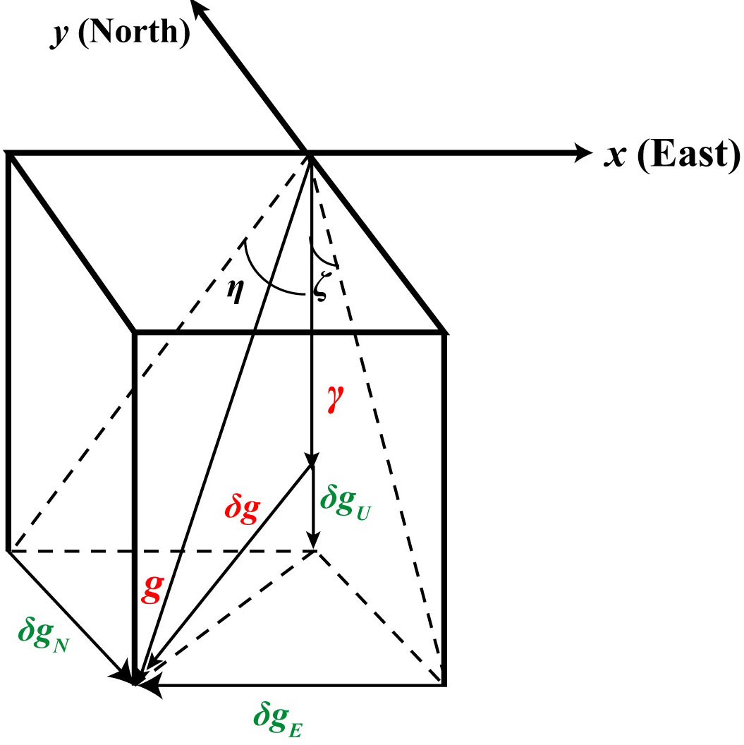
Figure 1 Definition of gravity disturbance vector.

The actual gravity differs from normal gravity owing to the existence of a vertical deflection. As shown in Figure 1, ζ is the meridian component of the DOV and η is the prime vertical component of the DOV. The horizontal gravity disturbance components on the x and y axes are negative when η and ζ are positive. Then:

$\begin{array}{ll}\tan \zeta =-\frac{\delta g_N}{\gamma +\delta g_U}& (10)\end{array}$

$\begin{array}{ll}\tan \eta =-\frac{\delta g_E}{\gamma +\delta g_U}& (11)\end{array}$

Because the deflection of the vertical is small, it can be approximated by tanζ=ζ and tanη=η , in addition, the δg_U can generally be ignored:

$\begin{array}{ll}\delta g_N=-\gamma ·\zeta & (12)\end{array}$

$\begin{array}{ll}\delta g_E=-\gamma ·\eta & (13)\end{array}$

The horizontal gravity disturbance components are calculated according to the DOV in the meridian and prime vertical directions. With the continuous development of satellite altimetry, the accuracy of determining the DOV from the altimetry model has been improved. In this study, the horizontal gravity disturbance determined by the altimetry model was used to achieve INS gravity compensation. The calculation process for the horizontal gravity disturbance is presented in section 3.4.

2.2 Effect of gravity disturbance on initial alignment

The initial alignment for INS is generally performed under the static base condition, which consists of two steps: coarse alignment and fine alignment. We can only obtain a coarse attitude matrix using coarse alignment. A certain misalignment angle error is observed. Gravity disturbances can be ignored in coarse alignments. However, the influence of horizontal gravity disturbance should be considered in fine alignment. System errors are estimated and corrected using Kalman filtering. According to Eq. (6)–(8), the INS error equation with static base conditions can be expressed as:

$\begin{array}{ll}\{\begin{array}{l}\dot{\varphi }=-\varphi \times {\omega }_{ie}^n-{ϵ}^n\\ \delta {\dot{v}}^n=\varphi \times f^n-2{\omega }_{ie}^n\times \delta v^n+{\nabla }^n+\delta g^n\end{array}& (14)\end{array}$

The system filtering state-space of fine alignment can be defined as:

$\begin{array}{ll}X={[\begin{array}{ccc}\delta v_E& \delta v_N& \begin{array}{ccc}{\varphi }_E& {\varphi }_N& \begin{array}{ccc}{\varphi }_U& {\nabla }_E& \begin{array}{ccc}{\nabla }_N& {ϵ}_E& \begin{array}{cc}{ϵ}_N& {ϵ}_U\end{array}\end{array}\end{array}\end{array}\end{array}]}^T& (15)\end{array}$

According to Eq. (14), the fine alignment state-space model is constructed was follows:

$\begin{array}{ll}\dot{X}=FX+U+GW& (16)\end{array}$

where

$\begin{array}{ll}F=[\begin{array}{l}{\begin{array}{ccc}{M}_1& I_{2\times 2}& 0\end{array}}_{2\times 3}\\ \begin{array}{ccc}{M}_2& 0_{3\times 2}& -I_{3\times 3}\end{array}\\ \begin{array}{ccc}{0}_{5\times 5}& 0_{5\times 2}& 0_{5\times 3}\end{array}\end{array}]& (17)\end{array}$

$\begin{array}{ll}U={[\begin{array}{ccc}\delta g_E& \delta g_N& 0_{1\times 8}\end{array}]}^T& (18)\end{array}$

$\begin{array}{ll}G=[\begin{array}{l}\begin{array}{cc}{I}_{2\times 2}& 0_{2\times 3}\end{array}\\ \begin{array}{cc}{0}_{3\times 2}& -I_{2\times 3}\end{array}\\ \begin{array}{cc}{0}_{5\times 2}& 0_{5\times 3}\end{array}\end{array}]& (19)\end{array}$

$\begin{array}{ll}W={[\begin{array}{cc}{\text{w}}_{1\times 2}^{\nabla }& {\text{w}}_{1\times 3}^{ϵ}\end{array}]}^T& (20)\end{array}$

$\begin{array}{ll}{M}_1=[\begin{array}{ll}0 2{\omega }_{\text{ie}}\sin B0& 2{\omega }_{\text{ie}}\sin B0-\gamma 0\end{array}\begin{array}{c}-2{\omega }_{\text{ie}}\sin B0\gamma 0 0\end{array}]& (21)\end{array}$

$\begin{array}{ll}{M}_2=[\begin{array}{l}\begin{array}{ccc}0& 0& \begin{array}{ccc}\begin{array}{cc}& \end{array}0& \begin{array}{cc}& \end{array}{\omega }_{\text{ie}}\sin B& -{\omega }_{\text{ie}}cosB\end{array}\end{array}\\ \begin{array}{ccc}0& 0& -{\omega }_{\text{ie}}\sin B\begin{array}{ccc}& 0\begin{array}{cc}& \end{array}& 0\end{array}\end{array}\\ \begin{array}{ccc}0& 0& {\omega }_{\text{ie}}cosB\begin{array}{ccc}\begin{array}{ccc}& & 0\end{array}& & \begin{array}{ccc}& 0& \end{array}\end{array}\end{array}\end{array}]& (22)\end{array}$

where ${\text{w}}_{1\times 2}^{\nabla }$ and ${\text{w}}_{1\times 3}^{ϵ}$ are the white noise errors of the accelerometer and gyro.

Taking the velocity under the static base condition as the observation, the measurement equation of the system can be given by:

$\begin{array}{ll}V-\tilde{V}=[\begin{array}{cc}{I}_{2\times 2}& 0_{2\times 8}\end{array}]X+v& (23)\end{array}$

where I is unit matrix, V is the true velocity, $\tilde{V}$ the estimated velocity, and v the observation noise.

The initial alignment based on Kalman filtering takes the velocity as the measured value; therefore, the values related to velocity (vⁿ , $\delta {\dot{v}}^n$, and δvⁿ ) can be regarded as known values. Therefore, the velocity error δvⁿ in Eq. (14) can be obtained. Let $y=\delta {\dot{v}}^n+2{\omega }_{ie}^n\times \delta v^n$ be a combination of observable measurements; then, the velocity error equation can be expressed as:

$\begin{array}{ll}{y}_E=-\gamma {\varphi }_N+\delta g_E+{\nabla }_E^n& (24)\end{array}$

$\begin{array}{ll}{y}_N=\gamma {\varphi }_E+\delta g_N+{\nabla }_N^n& (25)\end{array}$

We can let y=0 be under a static base; therefore, the horizontal steady-state attitude error can be obtained from Eq. (24) and (25), as follows:

$\begin{array}{ll}\{\begin{array}{l}\varphi N=\frac{\delta g_E+{\nabla }_E^n}{\gamma }=\frac{{\nabla }_E^n}{\gamma }-\eta \\ {\varphi }_E=-\frac{\delta g_N+{\nabla }_N^n}{\gamma }=-\frac{{\nabla }_N^n}{\gamma }+\zeta \end{array}& (26)\end{array}$

Eq. (26) shows that the fine alignment of the INS depends mainly on the ∇ⁿ and horizontal gravity disturbance. The north gravity disturbance caused an east attitude error, and the east gravity disturbance caused a north attitude error. For a dual-axis rotary modulation INS, ∇ⁿ can be weakened by periodically rotating the inertial sensor along the rotation axis. Horizontal gravity disturbance is the main factor affecting fine alignment. Therefore, the horizontal gravity disturbance should be compensated for during the initial alignment.

2.3 Gravity disturbance compensation for dual-axis rotation modulation INS

The gravity compensation of the INS includes compensation in the initial alignment and the pure INS calculation. The gravity compensation in the pure INS calculation means that the gravity disturbance is compensated in the velocity in Eq. (1). For gravity compensation in the initial alignment, Eq. (16) and (23) are used to construct the fine alignment state-space model, and the initial alignment errors caused by gravity disturbances are estimated and corrected. The high-resolution horizontal gravity disturbance from the satellite altimetry marine gravity field model is provided to the INS for the mechanical arrangement in this study. The specific gravity compensation process is illustrated in Figure 2.

FIGURE 2

Figure 2 Gravity compensation procedure of dual-axis rotary modulation INS.

3 Analysis of the impact of gravity disturbance on INS

3.1 Initial alignment

A corresponding static-based simulation experiment is designed to analyze the impact of gravity disturbance on the initial alignment. The simulation conditions are as follows: gyro drift bias, 0.001°/h; accelerometer drift bias, 10 ug; INS sampling interval, 100 Hz. The static position is located at 111.8154° E and 20.7394° N, with a height of 0. The east and north gravity disturbance of static position are 34.92 mGal and −29.18 mGal (1 mGal = 10^-5 m²s^-2), respectively, which is determined by satellite altimetry model (the specific calculation for horizontal gravity disturbance is given in section 4). The corresponding DOV components in the prime vertical and meridian are −7.4” and 6.2”, respectively. The accelerometer and gyro data are obtained by simulation according to the static INS velocity increment, angular velocity increment law, and inertial sensor error parameter set.

The initial attitude misalignment angle is set to [0.5°, 0.5°, 0.5°]^T for fine alignment, the velocity error is set to 0.03 m/s, and the initial alignment time is 3600 s. Figures 3A, B show the east and north attitude errors before and after the gravity compensation, respectively, and show that the attitude error is affected by the gravity disturbance. After gravity compensation, the horizontal attitude error is weakened. The improvement in the amplitude of the attitude error accuracy after gravity compensation tended to be consistent with the DOV. The DOV components in the prime vertical cause north attitude errors, while the DOV components in the meridian cause east attitude errors. In addition, the gravity disturbance and accelerometer drift bias are superimposed, which jointly affected the initial alignment attitude. The accelerometer drift bias is well estimated for the two-axis rotary modulation INS. This indicates that the attitude error in the initial alignment is mainly caused by the DOV, which has become the main factor affecting the initial alignment attitude and must be compensated.

FIGURE 3

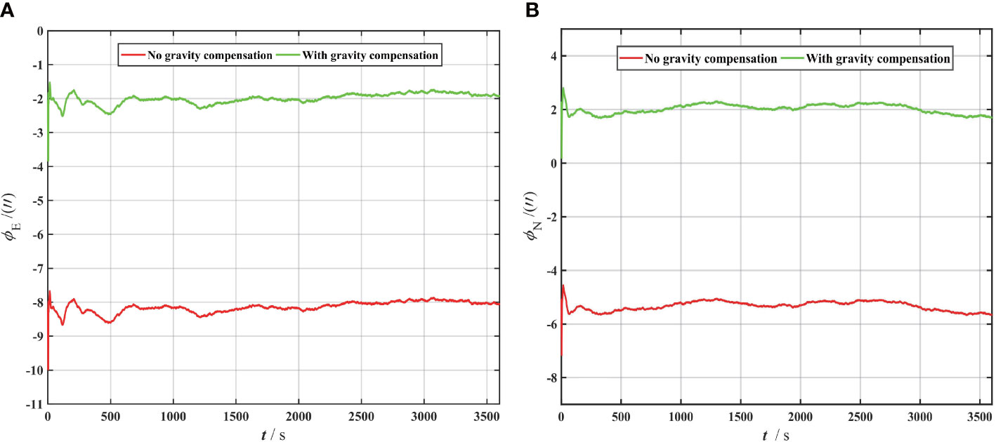
Figure 3 Alignment attitude error, (A) east, (B) north.

3.2 INS calculation

In the pure INS calculation, gravity disturbance first causes a velocity error, then further affects the position and attitude of the INS. In this section, the impact of gravity disturbance on the velocity and position is analyzed by ignoring the errors of the gyro, accelerometer, and attitude. The system error Eq. (6)–(7) can be solved analytically to quantitatively analyze the influence of the gravity disturbance. Figures 4A, B show the impacts of different gravity disturbances on the north velocity and position, respectively. Table 1 lists the maximum north position and velocity influence of different gravity disturbances on the INS. As shown in the Figures, the north position and velocity errors caused by gravity disturbance show periodic oscillation, and the error period of velocity and position is 84.4 min (Schuler period). Owing to the modulation of the Schuler period, the horizontal position and velocity errors caused by gravity disturbances are limited to a fixed amplitude. In addition, the results show that the amplitude of the position and velocity errors caused by the gravity disturbance is proportional to its amplitude. Ignoring the cross-coupling effect between the horizontal channels, the effects of gravity disturbance on the north and east positions is identical. For areas with obvious topographic variations, such as mountains or trenches, gravity disturbance has a greater impact on the INS.

FIGURE 4

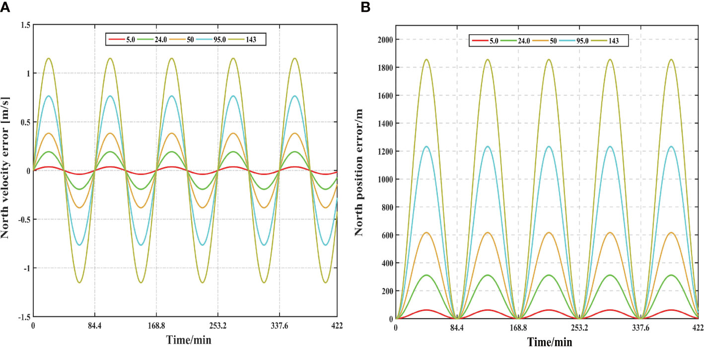
Figure 4 The error aroused by different gravity disturbance, (A) north velocity error, (B) north position error.

TABLE 1

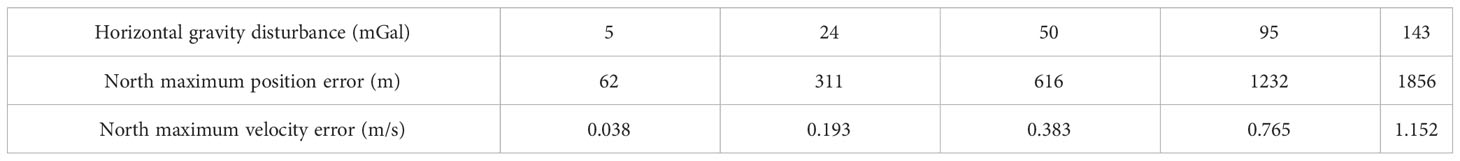
Table 1 The maximum influence of north gravity disturbance on north position and velocity.

The impact of gravity disturbance on the INS is analyzed above by assuming that the gravity disturbance is constant. In the actual survey line, the gravity disturbance changes from time to time. Therefore, we utilize an actual gravity survey line to study the impact of horizontal gravity disturbance on the INS. Figure 5 shows a gravity survey line with long-endurance (approximately 264 h), which starts from point A and ends at point B. The gravity sampling frequency is 1 Hz. The horizontal gravity disturbance on this gravity survey line is determined by the satellite altimetry model (see section 3.4 for the specific calculation), as shown in Figure 6. The gravity compensation for the INS is not only affected by the magnitude of the horizontal gravity disturbance but also by the horizontal gravity disturbance accuracy. Gaussian white noise with an expectation of 0 and a standard deviation of 3 mGal is added to the gravity disturbance on this trajectory to further analyze the effect of horizontal gravity disturbance accuracy. White Gaussian noise with a standard deviation of 3 mGal is added because the accuracy of the horizontal gravity disturbance determined by the altimetry model is approximately 1–3 mGal (Sandwell and Smith, 2014; Sandwell et al., 2014; Sandwell et al., 2021).

FIGURE 5

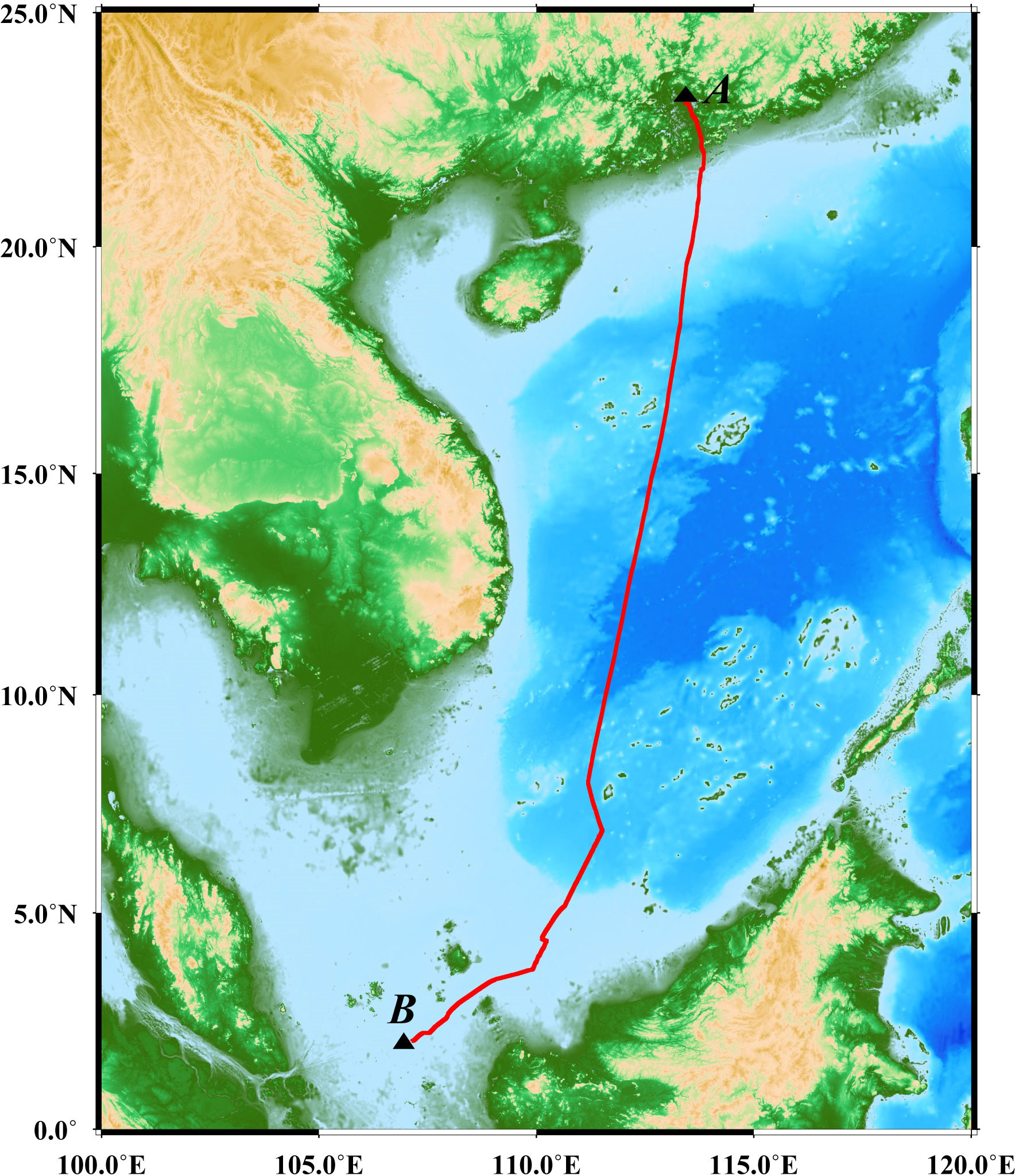
Figure 5 Marine gravity survey trajectory.

FIGURE 6

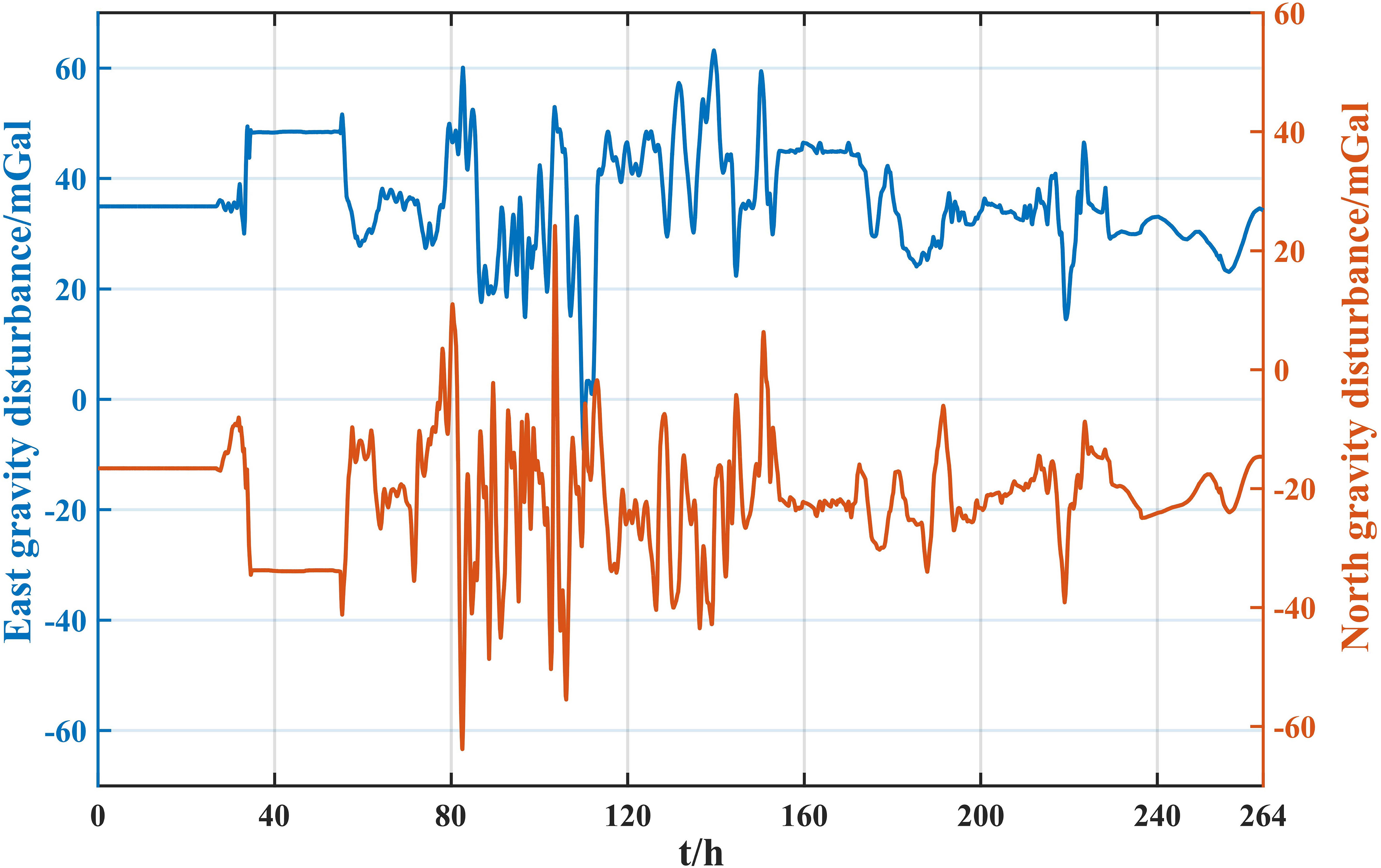
Figure 6 Horizontal gravity disturbance in gravity survey trajectory.

Figure 7 shows the maximum position error caused by the horizontal gravity disturbance in each Schuler cycle with and without noise. Table 2 shows the statistics of the maximum position error caused by the horizontal gravity disturbance for all the Schuler cycles. As shown in Figure 7, the maximum position errors are consistent in both cases (with and without noise). The maximum position error caused by gravity disturbance is mainly affected by the amplitude of gravity disturbance, and the horizontal gravity disturbance accuracy have little effect on gravity compensation. It can also be seen from Table 2 that the average maximum position error caused by horizontal gravity disturbance is also consistent in both cases (with and without noise). For satellite altimetry horizontal gravity disturbance with an accuracy of 1–3 mGal, the impact of the horizontal gravity disturbance accuracy could be ignored in gravity compensation. In addition, the average values of the east and north gravity disturbances on this survey line are 35.3 mGal and 21.3 mGal (after taking the absolute value), respectively. The maximum position error caused by the average gravity disturbance in a Schuler cycle is 535.9 m (theoretical analysis), and the average maximum position error caused by the horizontal gravity disturbance on this survey line in a Schuler cycle is 532.7 m (Table 2), which is consistent with both scenarios. This indicates that the average position influence of horizontal gravity disturbance is related to the average value of horizontal gravity disturbance on the trajectory.

FIGURE 7

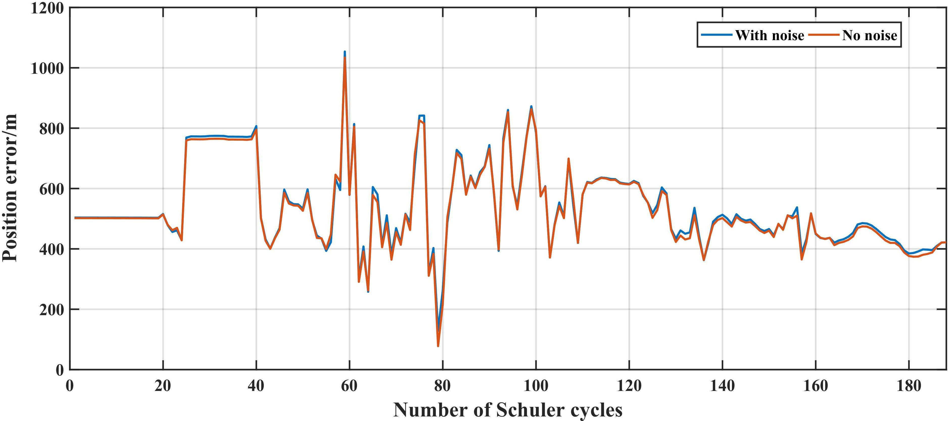
Figure 7 Maximum position error influence caused by horizontal gravity disturbance in each Schuler cycle.

TABLE 2

Table 2 Maximum error of INS caused by horizontal gravity disturbance in all Schuler cycles.

3.3 Frequency characteristics of INS affected by gravity disturbance

To analyze and obtain the frequency characteristics of the INS affected by gravity disturbance, the gravity disturbance is modeled as a Markov process (Jekeli, 2006). Therefore, the relationship between the horizontal gravity disturbance, underwater vehicle velocity V, spatial wavelength of gravity disturbance, and position error caused by horizontal gravity disturbance is established. The calculation of the root mean square value for gravity disturbance is a key factor in determining the relationship between the spatial wavelength, underwater vehicle velocity V, and position error. The root mean square value of the horizontal gravity disturbance can be determined according to the relationship between the horizontal gravity disturbance and DOV. Therefore, the global root mean square value of the DOV is calculated using the EIGEN_6C4 model in this study (Ustun and Abbak, 2010). The global root mean square of the DOV is approximately ±7.08” (equivalent to a horizontal gravity disturbance of ±33.57 mGal), as shown in Figure 8. Finally, the relationship between the horizontal gravity disturbance, underwater vehicle velocity V, spatial wavelength of gravity disturbance, and position error is determined, as shown in Figure 9.

FIGURE 8

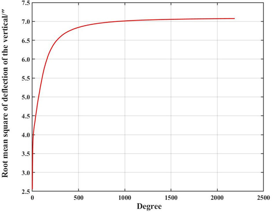
Figure 8 Root mean square of deflection of the vertical.

FIGURE 9

Figure 9 Relationship between position error (root mean square value) and spatial wavelength caused by horizontal gravity disturbance at different velocities.

As shown in Figure 9, the position error is mainly caused by the medium-long wavelength (medium-low frequency) of the horizontal gravity disturbance when the underwater vehicle velocity is high. With a decrease in underwater vehicle velocity, the influence of the short-wavelength (high-frequency) of the horizontal gravity disturbance on the INS position become increasingly significant. The velocity of an underwater vehicle is generally 10–25 kn (1 kn = 1 n mile/h), and the spatial wavelength of the horizontal gravity disturbance, which has the greatest influence on the INS position, is approximately 5−10 km. For an underwater vehicle with a lower velocity, the gravity disturbance high-frequency signal has an increasingly marked influence on the INS. The maximum spatial wavelength of the degree 2190 gravity field model is 10 km. High-degree GFM (i.e. EGM2008 or EIGEN_6C4) can satisfy the requirements of gravity compensation for high-speed underwater vehicles (V > 50 km/h). However, for underwater vehicles with low-speed, determining the high-frequency signal of horizontal gravity disturbance is the key to further promoting gravity compensation accuracy, and the satellite altimetry gravity field model provides an effective means to determine high-resolution horizontal gravity disturbance.

3.4 Horizontal gravity disturbance for the China Sea and Western Pacific region

The maximum effect of the horizontal gravity disturbance on the INS position is proportional to its amplitude. For areas with obvious topographic fluctuations, such as seamount ranges or trenches, the horizontal gravity disturbance is greater. The distribution of horizontal gravity disturbance in the China Sea and Western Pacific region and its impact on INS are analyzed using a satellite altimetry model. The seafloor topography in the China Sea and Western Pacific region is complex and contains a large number of islands, reefs, submarine plains, and trenches, which can accurately reflect the distribution of horizontal gravity disturbance under different topographies.

Figure 10A shows the component of the DOV in the prime vertical with a spatial resolution of 1’ × 1’ in the China Sea and Western Pacific region obtained based on the altimetry model. Figure 10B shows the component of the DOV in the meridian with a spatial resolution of 1’ × 1’ in the China Sea and Western Pacific region obtained based on the altimetry model. This gridded marine DOV data is one of the most advanced marine gravity databases, derived from satellite altimetry from 1997 to 2019 with a spatial resolution of 1’ × 1’, and can better represent the marine high-frequency gravity field signal (Sandwell and Smith, 2014; Sandwell et al., 2014; Sandwell et al., 2021). The latest marine DOV data (version SIO V30.1 from the Scripps Institution of Oceanography (SIO) at the University of California, San Diego) is used in this study. As can be seen from Figures 10A, B, the DOV in the China Sea and Western Pacific region is generally between a few to tens of arcseconds. In areas where the seafloor topography changes dramatically, the maximum DOV can reach 80 arcseconds. According to Eq. (12) and (13), the horizontal gravity disturbance in the China Sea and the western Pacific region can be calculated. Figure 10C shows the east gravity disturbance with a spatial resolution of 1’ × 1’. Figure 10D shows the north gravity disturbance with a spatial resolution of 1’ × 1’. The horizontal gravity disturbance in the China Sea and Western Pacific region generally ranges from a few to several hundred milligals, and the maximum horizontal gravity disturbance reaches several hundred milligals in areas where the seafloor topography changes dramatically. Four regions are divided to analyze the distribution of horizontal gravity disturbances on four important channels and their influence on the INS: region A is the South China Sea, region B is the East China Sea, region C is the Sea of Japan, and region D is a part of the western Pacific (Figures 10C, D). The size of each of the four regions was 10° × 10°. The influence of the average horizontal gravity disturbance in four regions on the maximum position influence of the INS in the Schuler period was analyzed, the results of which are presented in Table 3. It is worth noting that the range and average value of east and north gravity disturbance in Table 3 are statistical results of absolute values.

FIGURE 10

Figure 10 The DOV and gravity disturbances from SIO V30.1 model, (A) Component of the DOV in prime vertical, (B) component of the DOV in meridian, (C) east gravity disturbances, and (D) north gravity disturbances.

TABLE 3

Table 3 Horizontal gravity disturbance and maximum position influence caused by average gravity disturbance on INS in a Schuler period (δg_N−Scope and δg_E−Scope show distribution range of north and east gravity disturbance, and δP_Max show influence of mean gravity disturbance on INS position).

From Table 3, we can see that the horizontal gravity disturbance range in regions A, B and C is smaller than that in region D, and the maximum horizontal gravity disturbance in region D could reach several hundred milligals owing to the presence of trenches. The average gravity disturbance in regions A, B, and C had a maximum impact on the INS position of several hundred meters in the Schuler period, while the average gravity disturbance in area D had a maximum impact on the INS position of more than 1000 m in the Schuler period. In particular, in areas with rugged topography, such as trenches and seamounts, gravity disturbance has a maximum impact on the INS position error of several thousand meters in a Schuler period. For areas with a complex seafloor topography, the impact of high-frequency horizontal gravity disturbance cannot be ignored, as the gravity compensation of INS based on high-degree GFMs often leads to a loss of compensation accuracy. The gravity compensation of high-precision INS can be achieved using a high-precision marine horizontal gravity disturbance from the SIO V30.1 model.

4 Marine gravity compensation experiment

A marine dynamic shipborne test is conducted in the South China Sea to verify the effectiveness of gravity compensation. A two-axis rotary modulation laser INS, which contained three laser gyroscopes and three quartz flexible accelerometers, is used. The gyro drift bias is better than 0.001°/h and the accelerometer drift bias is lower than 10 ug. The INS provides 500 Hz measurements. Differential GNSS is used to obtain the reference position information for the ship-based experiment. The horizontal positioning accuracy of the GNSS is better than 1 m, and the GNSS could provide position information at 1 Hz. The trajectory of the ship-mounted experiment is shown in Figure 11, which operates statically for approximately 4 h at the starting point, then dynamically for approximately 10.5 hours. The INS operates for approximately 14.5 hours in total.

FIGURE 11

Figure 11 Trajectory of marine experiment.

4.1 Determination of horizontal gravity disturbance

The horizontal gravity disturbance is calculated using the SIO V30.1 model (section 3.4). For comparative analysis, the high-degree EIGEN_6C4 model is used to determine the horizontal gravity disturbance (Barthelme, 2013; Ince et al., 2019). Figure 12 shows the horizontal gravity disturbance on the ship-based experimental trajectory, δg_{E−SIO V30.1} shows that the east gravity disturbance determined by the SIO V30.1 model, δg_E−GGM is the east gravity disturbance determined by the EIGEN_6C4 model, δg_{N−SIO 30.1} shows that the north gravity disturbance determined by the SIO V30.1 model, and δg_N−GGM is the north gravity disturbance determined by the EIGEN_6C4 model. The maximum east gravity disturbance on the experimental trajectory is approximately 50 mGal and the maximum north gravity disturbance on the experimental trajectory is approximately −30 mGal.

FIGURE 12

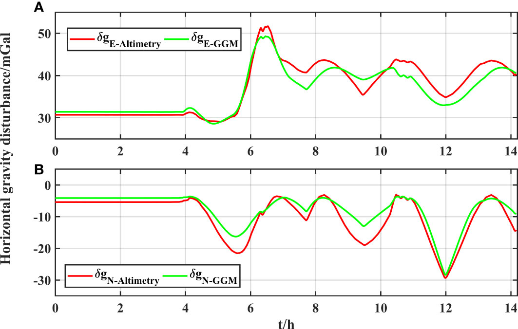
Figure 12 Horizontal gravity disturbance along trajectory of ship, (A) east gravity disturbance and (B) north gravity disturbance.

4.2 Gravity compensation results

The horizontal gravity disturbance calculated above is used to achieve gravity compensation for the dual-axis rotation modulation INS. The specific gravity compensation process is illustrated in Figure 2 Gravity compensation includes compensation in the initial alignment and pure INS calculations. The two-axis rotary modulation INS is performed for approximately 50 min of fine alignment and accomplished gravity compensation in fine alignment. Then, the gravity compensation is completed in the pure INS calculation.

For comparison and analysis, two gravity compensation methods are adopted. The first method utilizes the gravity disturbance calculated by the EIGEN_6C4 model, while the second utilizes the gravity disturbance from the SIO V30.1 model. The longitude, latitude, and position errors with and without gravity disturbance compensation are shown in Figures 13A–C, respectively. Both compensation methods are found to weaken the INS error oscillation. The second compensation method further weakens the error oscillation of the INS owing to the higher-frequency horizontal gravity disturbance calculated by the SIO V30.1 model (satellite altimetry model). Figure 14 shows the improvement in the INS positioning accuracy after gravity compensation using two different gravity compensation methods. Table 4 shows the maximum performance improvement of the INS using the two different gravity compensation methods. After gravity compensation by the first gravity compensation method, the longitudinal performance of the INS is improved by 152 m, the latitude performance is improved by 311 m, the position performance is improved by 309 m, and the ranges of longitude, latitude, and position are improved by 17.6%, 17.5%, and 16.6%, respectively. After using the second method for gravity compensation, the longitude performance of the INS is improved by 161 m, the latitude performance is improved by 334 m, the position performance is improved by 335 m, and the range of longitude, latitude, and position are improved by 18.5%, 18.7%, and 17.9%, respectively. These results indicate that gravity compensation can further improve the performance of high-precision INS. Compared to the high-degree gravity field model, the gravity compensation performance of the satellite altimetry model is better because it contained a higher-frequency gravity field signal.

FIGURE 13

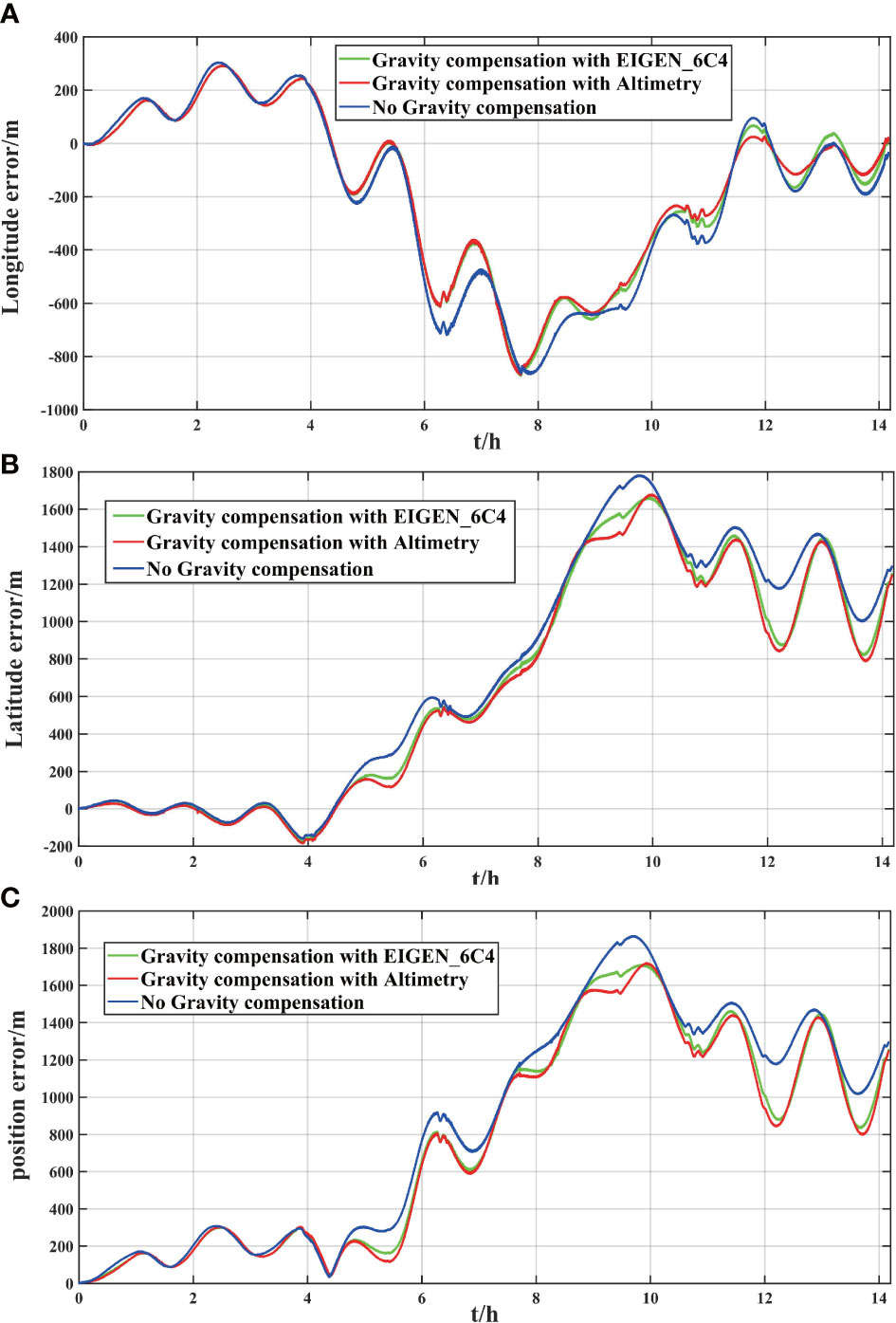
Figure 13 (A) Longitude error, (B) Latitude error, and (C) Position error.

FIGURE 14

Figure 14 Positioning accuracy improvement corresponding to different methods.

TABLE 4

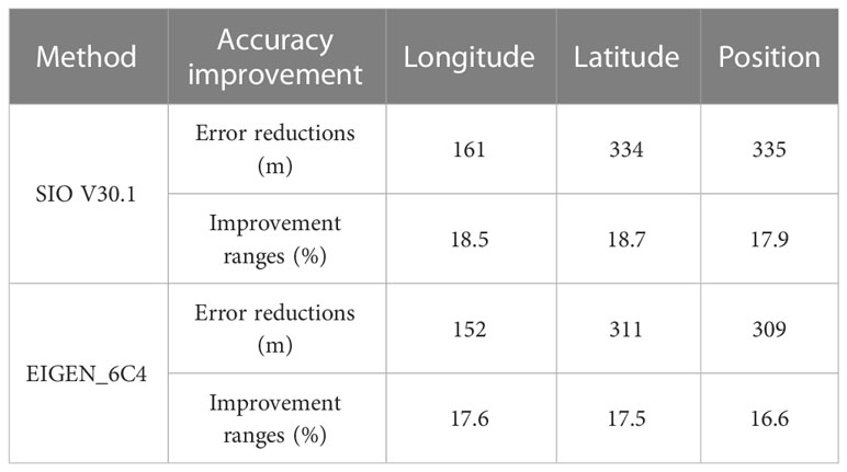
Table 4 Improvement of maximum positioning accuracy using two different gravity compensation methods.

In the gravity compensation of a high-precision INS, the horizontal gravity disturbance determined by the satellite altimetry model could be used to achieve gravity compensation, which can improve the mechanical arrangement of the INS. In particular, for areas with large topographic changes (such as trenches or seamounts), the impact of high-frequency gravity disturbances caused by seafloor topography must be considered. As discussed in section 3.3, the influence of the higher-frequency signal of the horizontal gravity disturbance on the INS position is increasingly significant for low-speed underwater vehicles. However, the high-degree gravity field model (EGM2008 or EIGEN_6C4) could not effectively represent higher-frequency gravity field signals because the spatial wavelength of these models is limited. The satellite altimetry model (SIO V30.1) can effectively represent the high-frequency gravity field signal, which meets the requirements of gravity compensation.

Tie et al. (2017) studied the performance of gravity compensation in initial alignment and pure INS calculations. Their results showed that only gravity compensation in the pure INS calculation improved the performance of INS, while gravity compensation in both the initial alignment and pure INS calculation worsened the performance of INS. The main reason for this is that accelerometer drift and gravity disturbances are coupled. For a dual-axis rotary modulation INS, the accelerometer drift bias can be estimated well, and the coupling effect can be ignored in gravity compensation. To further prove the effectiveness of gravity compensation simultaneously in the initial alignment and pure INS calculations, two gravity compensation strategies are adopted. The first strategy is comprised of gravity compensation only in the pure INS calculation, while the second strategy involves simultaneous gravity compensation in the initial alignment and pure INS calculation. The SIO V30.1 model is utilized for gravity compensation. The position errors from the two gravity compensation strategies are compared in Figure 15. Gravity compensation using the second strategy is found to have a minimum position error, which indicates that gravity compensation should be carried out in the initial alignment and pure INS calculation. Chang et al. (2019) also found that the gravity compensation of high-precision INS needed to be compensated for both the initial alignment and the pure INS calculation. Therefore, for a high-precision INS, when the accelerometer drift bias is fully calibrated or modulated, the positioning accuracy of the INS could be further improved by achieving gravity compensation in the initial alignment and pure INS calculation. If the accelerometer drift bias is not fully calibrated or modulated, the horizontal gravity disturbance and accelerometer drift bias will be coupled in gravity compensation, which may not be effective.

FIGURE 15

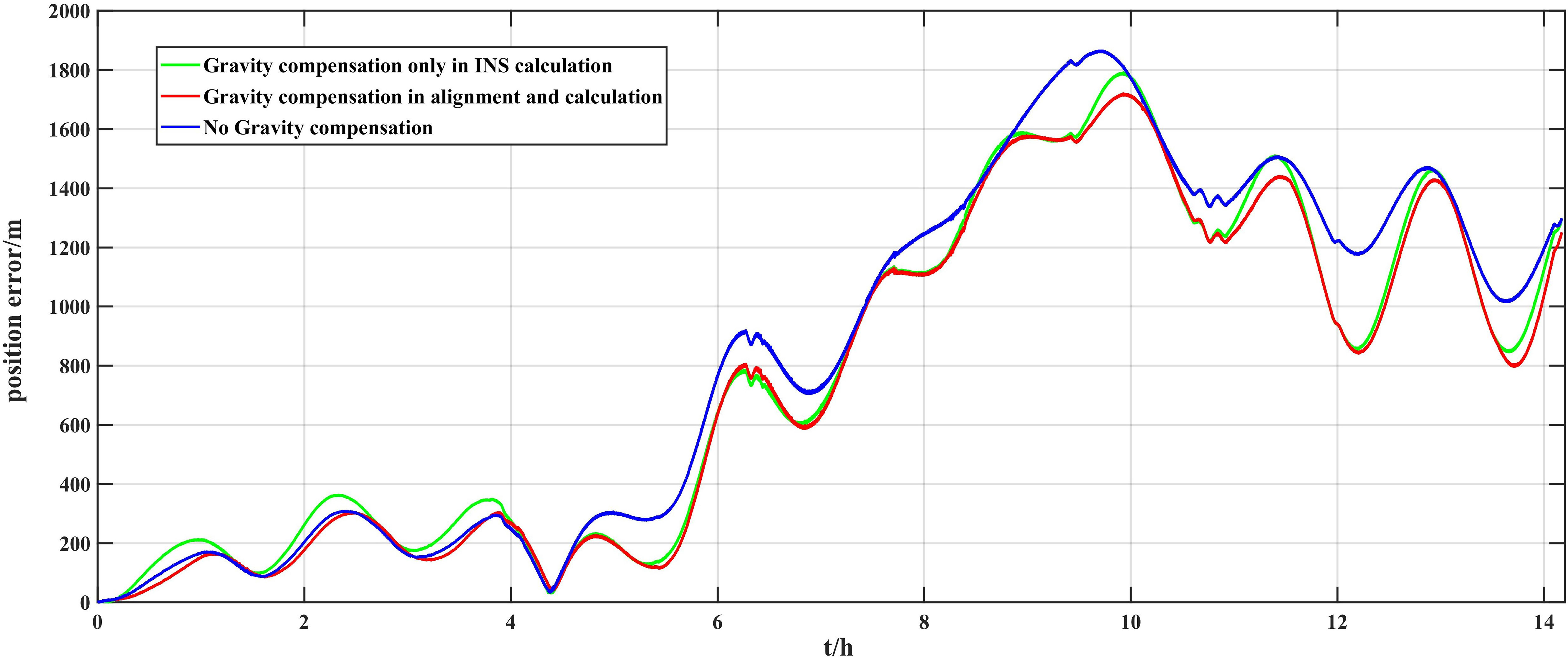
Figure 15 Position error caused by different compensation strategies.

5 Conclusion

Gravity disturbance compensation is essential for further improving the positioning accuracy of the INS. In this study, the error and frequency characteristics of INS caused by gravity disturbances are investigated. The results show that the east gravity disturbance affects the north attitude, and the north gravity disturbance affects the east attitude in the initial alignment. In the pure INS calculation, the horizontal gravity disturbance causes a navigation error in the form of Schuler oscillation. The position error is mainly caused by the medium-long wavelength (medium-low frequency) gravity disturbance when the underwater vehicle velocity is larger. With a decrease in underwater vehicle velocity, the influence of the short-wavelength (high-frequency) of gravity disturbance become increasingly significant.

The distribution of horizontal gravity disturbance in the China Sea and Western Pacific region and its impact on INS are analyzed based on a satellite altimetry model (SIO V30.1). Four regions are divided to analyze the distribution of horizontal gravity disturbances on four important channels and their influence on the INS. The results show that the average gravity disturbance in the South China Sea, the East China Sea, and the Sea of Japan have a maximum impact on the INS position of several hundred meters in the Schuler period, and the average gravity disturbance in the western Pacific has a maximum impact on the INS position of more than 1000 m in the Schuler period. In particular, in areas with rugged topography, such as trenches and seamounts, gravity disturbance is found to have a maximum impact on the INS position error of several thousand meters in a Schuler period.

Finally, the dynamic ship-mounted experiment verified the effectiveness of the satellite altimetry model (SIO V30.1) in achieving gravity compensation. After gravity compensation using the altimeter model, the positioning accuracy has been improved by 18%. The satellite altimetry model is able to effectively represent the high-frequency gravity field signal, which meets gravity compensation requirements. In particular, for regions with large topographic changes (e.g. trenches or seamounts), the impact of high-frequency gravity disturbances caused by seafloor topography must be considered.

Data availability statement

The original contributions presented in the study are included in the article/supplementary material. Further inquiries can be directed to the corresponding authors.

Author contributions

LW, LB and YW conceived the study. The data processing and collection were conducted by QL, HL and BW. The analysis of the results was implemented by PZ, LB, and LW. And the initial draft of the manuscript was written by PZ with improvements and substantial edits from all authors. All authors contributed to the article and approved the submitted version.

Funding

This work was supported by the National Natural Science Foundation of China (grant nos. 42192535, 41931076, 42274116, and 42174102), and the Basic Frontier Science Research Program of the Chinese Academy of Sciences (grant no. ZDBSLY-DQC028).

Acknowledgments

We acknowledge David Sandwell, University of California, San Diego, for providing radar altimeter-derived gravity data used in this study. We also acknowledge the International Centre for Global Earth Models (ICGEM) for providing us with the gravity field model.

Conflict of interest

The authors declare that the research was conducted in the absence of any commercial or financial relationships that could be construed as a potential conflict of interest.

Publisher’s note

All claims expressed in this article are solely those of the authors and do not necessarily represent those of their affiliated organizations, or those of the publisher, the editors and the reviewers. Any product that may be evaluated in this article, or claim that may be made by its manufacturer, is not guaranteed or endorsed by the publisher.

References

Andersen O. B., Knudsen P., Berry P. A. M. (2010). The DNSC08GRA global marine gravity field from double retracked satellite altimetry. J. Geod. 84 (3), 191–199. doi: 10.1007/s00190-009-0355-9

CrossRef Full Text | Google Scholar

Bao L., Xu H., Li Z. (2013). Towards a 1 mGal accuracy and 1 min resolution altimetry gravity field. J. Geod. 87 (10-12), 961–969. doi: 10.1007/s00190-013-0660-1

CrossRef Full Text | Google Scholar

Barthelme F. (2013). Definition of functionals of the geopotential and their calculation from spherical harmonic models–theory and formulas used by the calculation service of the international centre for global earth models (ICGEM) (Potsdam, Germany: GFZ German Research Centre for Geosciences Report No: STR09/02).

Google Scholar

Chang L., Qin F., Wu M. (2019). Gravity disturbance compensation for inertial navigation system. IEEE Trans. Instrum. Meas. 68 (10), 3751–3765. doi: 10.1109/TIM.2018.2879145

CrossRef Full Text | Google Scholar

Denker H. (2013). “Regional gravity field modeling: Theory and practical results,” in Sciences of geodesy – II. innovations and future developments. Ed. Xu G. (Berlin: Springer), 185–182.

Google Scholar

Förste C., Bruinsma S. L., Abrikosov O., Lemoine J. M., Marty J. C., Flechtner F., et al. (2014). Data from: EIGEN-6C4-The latest combined global gravity field model including GOCE data up to degree and order 2190 of GFZ potsdam and GRGS toulouse. GFZ data service. doi: 10.5880/icgem.2015.1

CrossRef Full Text | Google Scholar

Gelb A., Levine S. A. (1969). Effect of deflections of the vertical on the performance of a terrestrial inertial navigation system. J. Spacecraft Rockets 6 (9), 978–984.

Google Scholar

Hanson P. O. (1988). “Correction for deflections of the vertical at the runup site,” in Proceedings of the IEEE position location and navigation symposium 1988. (Orlando, FL, USA: IEEE PLANS), 288–296.

Google Scholar

Heller W. G., Jordan S. K. (2015). Error analysis of two new gradiometer-aided inertial navigation systems. J. Spacecraft Rockets 13 (6), 340.

Google Scholar

Hofmann-Wellenhof B., Moritz H. (2006). Physical geodesy (Wien: Springer).

Google Scholar

Ince E. S., Barthelmes F., Reißland S., Elger K., Förste C., Flechtner F., et al. (2019). ICGEM-15 years of successful collection and distribution of global gravitational models, associated services, and future plans. Earth Syst. Sci. Data 11 (2), 647–674. doi: 10.5194/essd-11-647-2019

CrossRef Full Text | Google Scholar

Jekeli C. (2006). Precision free-inertial navigation with gravity compensation by an onboard gradiometer. J. Guid. Contral Dynam. 29 (3), 704–713. doi: 10.2514/1.15368

CrossRef Full Text | Google Scholar

Jekeli C., Lee J., Kwon J. (2007). Modeling errors in upward continuation for INS gravity compensation. J. Geod. 81 (5), 297–309. doi: 10.1007/s00190-006-0108-y

CrossRef Full Text | Google Scholar

Jordan S. (1973). Effects of geodetic uncertainties on a damped inertial navigation system. IEEE Trans. Aero. Elec. Sys AES-9 (5), 741–752. doi: 10.1109/TAES.1973.309774

CrossRef Full Text | Google Scholar

Kwon J. H., Jekeli C. (2005). Gravity requirements for compensation of ultra-precise inertial navigation. J. Navigation 58 (3), 479–492. doi: 10.1017/S0373463305003395

CrossRef Full Text | Google Scholar

Pavlis N. K., Holmes S. A., Kenyon S. C., Factor J. F. (2012). The development and evaluation of the earth gravitational model 2008(EGM2008). J. Geophys. Res. 117, B04406. doi: 10.1029/2011JB008916

CrossRef Full Text | Google Scholar

Sandwell D. T., Harper H., Tozer B., Smith W. (2021). Gravity field recovery from geodetic altimeter missions. Adv. Space Res. 68 (2), 1059–1072. doi: 10.1016/j.asr.2019.09.011

CrossRef Full Text | Google Scholar

Sandwell D. T., Müller R. D., Smith W. H., Garcia E., Francis R. (2014). New global marine gravity model from CryoSat-2 and Jason-1 reveals buried tectonic structure. Science 346 (6205), 65–67.

PubMed Abstract | Google Scholar

Sandwell D. T., Smith W. H. F. (2014). Slope correction for ocean radar altimetry. J. Geod. 88 (8), 765–771. doi: 10.1007/s00190-014-0720-1

CrossRef Full Text | Google Scholar

Simav M. (2020). The use of gravity reductions in the indirect strapdown airborne gravimetry processing. Surv. Geophys. 41 (4):1029–1048. doi: 10.1007/s10712-020-09596-3

CrossRef Full Text | Google Scholar

Tie J., Cao J., Wu M., Lian J., Cai S., Wang L. (2018). Compensation of horizontal gravity disturbances for high precision inertial navigation. Sensors 18 (3), 906. doi: 10.3390/s18030906

PubMed Abstract | CrossRef Full Text | Google Scholar

Tie J., Wu M., Cao J., Lian J., Cai S. (2017). “The impact of initial alignment on compensation for deflection of vertical in inertial navigation,” in Proceedings of 8th IEEE International Conference on Cybernetics & Intelligent Systems. (Ningbo, China: IEEE). 381–386.

Google Scholar

Tscherning C., Rapp R. (1974). Closed covariance expressions for gravity anomalies, geoid undulations, and deflections of the vertical implied by anomaly degree variance models (Department of Geodetic Science and Surveying, The Ohio State University Report No: 208).

Google Scholar

Ustun A., Abbak R. (2010). On global and regional spectral evaluation of global geopotential models. J. Geophys. Eng. 7 (4), 369. doi: 10.1088/1742-2132/7/4/003

CrossRef Full Text | Google Scholar

Wang J., Yang G., Li X., Zhou X. (2016). Application of the spherical harmonic gravity model in high precision inertial navigation systems. Meas. Sci. Technol. 27 (9), 095103. doi: 10.1088/0957-0233/27/9/095103

CrossRef Full Text | Google Scholar

Wen J., Liu J., Jiao M., Kou K. (2020). Analysis and on-line compensation of gravity disturbance in a high-precision inertial navigation system. GPS Solut. 24, 83. doi: 10.1007/s10291-020-00998-9

CrossRef Full Text | Google Scholar

Wen H., Lu Q., Huang K. (2009). Rotation scheme design for rotary optical gyro SINS. J. Chin. Inertial Technol. 17 (1), 8–14.

Google Scholar

Wu Q., Li K. (2019). An inertial device biases on-line monitoring method in the applications of two rotational inertial navigation systems redundant configuration. Mech. Syst. Signal Process 120, 133–149. doi: 10.1016/j.ymssp.2018.10.005

CrossRef Full Text | Google Scholar

Yuan B., Liao D., Han S. (2012). Error compensation of an optical gyro INS by multi-axis rotation. Meas. Sci. Technol. 23 (2), 91–95. doi: 10.1088/0957-0233/23/2/025102

CrossRef Full Text | Google Scholar

Zhou X., Yang G., Wang J., Li. J. (2016). An improved gravity compensation method for high-precision free-INS based on MEC-BP-AdaBoost. Meas. Sci. Technol. 27 (12), 125007. doi: 10.1088/0957-0233/27/12/125007

CrossRef Full Text | Google Scholar

Zhou X., Yang G., Wang J., Wen Z. (2018). A combined gravity compensation method for INS using the simplified gravity model and gravity database. Sensors 18 (5), 1552. doi: 10.3390/s18051552

PubMed Abstract | CrossRef Full Text | Google Scholar