Best practices for operating underwater gliders in Atlantic Canada

1 Introduction

Ocean observations in the Northwest Atlantic are vital for many different reasons: (i) there is a very productive and active fishery throughout the region (Fisheries and Oceans Canada, 2021), (ii) trans-Atlantic shipping uses this region to reach New England and through the Gulf of St. Lawrence to central Canada (Simard et al., 2010), (iii) it is a crucial area of importance to global climate (Broecker et al., 1991; Sabine et al., 2004; Landschützer et al., 2014; Lozier et al., 2019), aquatic ecosystems science (de Young and Rose, 1993; de Young et al., 1999; Lotze and Milewski, 2004; Baumgartner et al., 2018) and (iv) it is a region of active offshore oil exploration and exploitation and strategic interests and responsibilities to people calling Canada their home (Macdonald, 1966; Crickard, 1995; Ricketts and Harrison, 2007; Whoriskey et al., 2017).

Several critical regional observing efforts have been developed to meet scientific and societal needs and contribute to international and national ocean observing strategies. These observing programs are collaborative efforts between academic institutions, governments, nonprofits, commercial entities, and defense sectors. Traditionally, programs such as the Atlantic Zone Monitoring Program [AZMP; Therriault et al. (1998)], supported by Fisheries and Oceans Canada (DFO), utilize vessels to collect data and report on various program objectives. Programs relying on ships are increasingly complemented by autonomous observations such as automatic buoys, Argo (Roemmich et al., 2009) floats, gliders (Davis et al., 2002; Rudnick et al., 2004), and, to a lesser degree, moorings.

Gliders – winged cylinder-shaped autonomous underwater vehicles (AUV) – are an emerging platform for ocean observations with technology adoption in Atlantic Canada starting as early as 2005 and continuing to this day. Gliders here refer exclusively to underwater profiling buoyancy-driven underwater vehicles. Some gliders can also operate in propelled modes via the use of a hybrid thruster (Claus et al., 2010). Thrusters can increase the horizontal speed of gliders, thereby increasing the operating envelope of gliders and blurring the line between profiling gliders and other powered AUVs that exclusively navigate in propelled modes. Other vehicles, referred to as gliders, are used in Atlantic Canada, such as wave gliders. This paper will only discuss underwater profiling gliders primarily deployed by academic and governmental groups. Gliders can fill ocean observing gaps, such as in regions where Argo floats do not have coverage and will rapidly drift away (e.g., continental shelf or boundary currents) and with higher sampling frequency (10 days vs a few hours) though with reduced duration (Liblik et al., 2016; Testor et al., 2019). Gliders may also complement moored observations (e.g. OOI Pioneer Array (Trowbridge et al., 2019)).

One challenge for potential users interested in adopting gliders as a platform is that the background knowledge on gliders has not been readily available in the refereed literature. There are few reports and papers in the refereed literature discussing the operations of gliders in Atlantic Canada and operational considerations for gliders in general. Helpful forums do exist specific to glider data and best practices such as the Ocean Gliders Community Github page (https://github.com/OceanGlidersCommunity). Other knowledge sharing groups such as the US Underwater Glider Group (UG2) also offer new ways to exchange information. In particular, their recent UG2 Slack channel offers effective ways to exchange knowledge among gliders users. This paper shares first hand glider experience from operating gliders in Atlantic Canada since 2005, highlighting challenges in sustaining glider observations. This paper expands the scope of a previous group paper highlighting lessons learned operating gliders in Atlantic Canada (Davis et al., 2018). The discussion focuses on practical issues and lessons learned from glider operations in this part of the ocean that should be relevant to users in other regions.

2 Glider operators in Atlantic Canada

Underwater profiling glider (or simply gliders hereafter) operations now take place regularly in all regions of Atlantic Canada (Figure 1) and through various groups with different and similar capabilities (Table 1). Use of gliders in Atlantic Canada started in 2005 at the National Research Council (NRC) in St. John’s, Newfoundland and Labrador (NL), in 2010 in Halifax, Nova Scotia (NS) with the Coastal Environmental Observation Technology and Research (CEOTR) Group and in 2017 with DFO. Here we describe each of these glider groups and their main projects and study areas within Atlantic Canada.

FIGURE 1

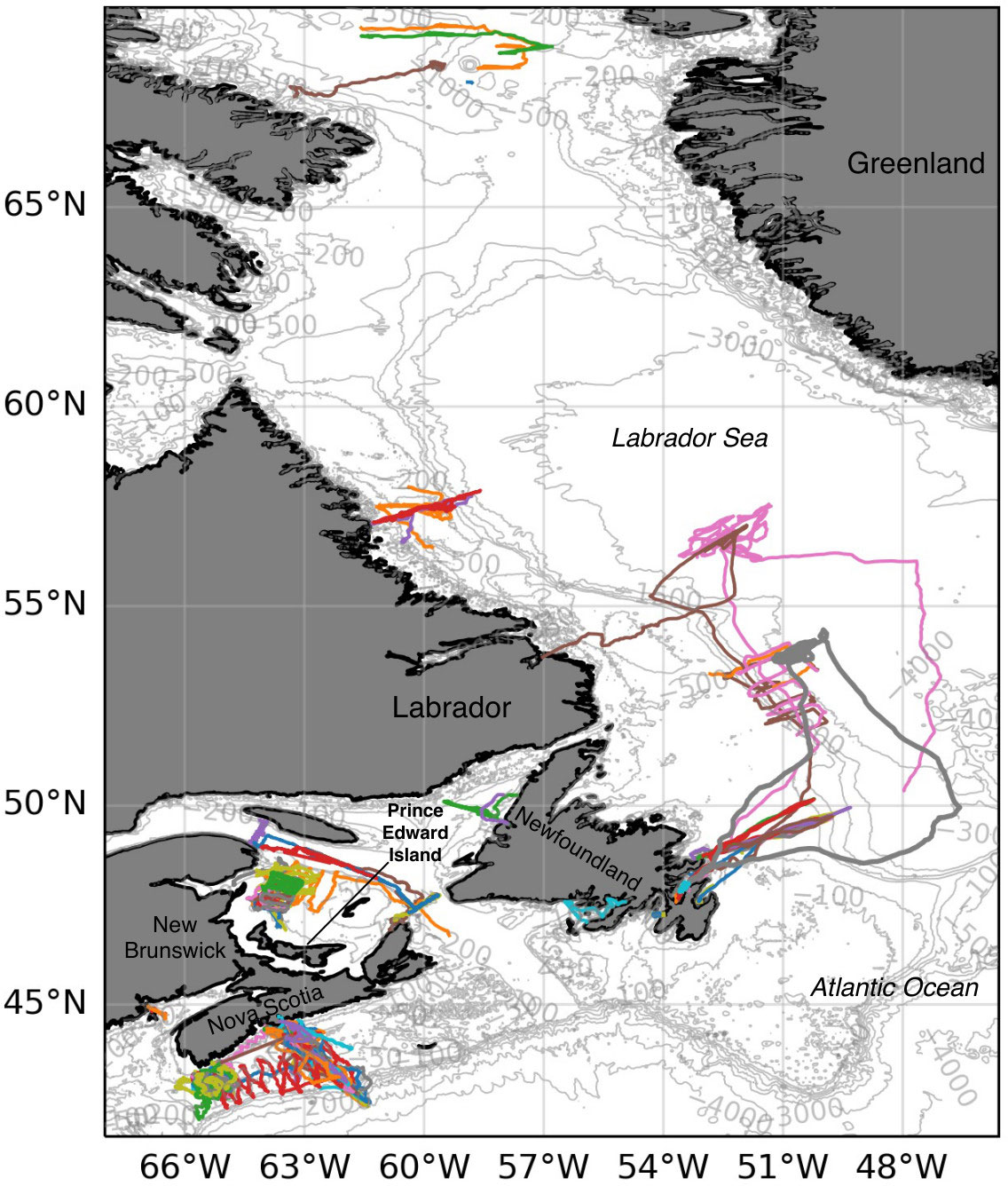
Figure 1 Map showing Atlantic Canadian glider deployments for the period 2006–2023. Different colors are used for individual deployments. Bathymetric contours are displayed in light grey with data from GEBCO (2022).

TABLE 1

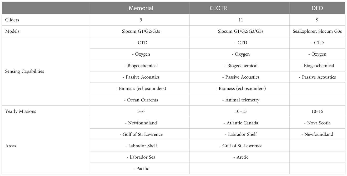
Table 1 Glider capabilities in Atlantic Canada.

2.1 Memorial University glider group

Glider operations at Memorial began in 2005 using four Slocum gliders (Jones et al., 2014) looking at developing new glider capabilities (thrusters) and sensor integrations (sonars) to expand their capabilities for underwater navigation. For example, Zhou et al. (2019) added a scanning sonar using the glider to map the submerged portion of an iceberg. Earlier, Zhou et al. (2017) developed a short-baseline navigation system to enhance the positional accuracy of the glider to enable detailed mapping of objects like icebergs. Claus and Bachmayer (2015) worked on terrain-aided navigation using fluxgate approaches and depth operated controllers. Claus et al. (2010) brought the integration and controllers for thrusters on Slocum gliders that allowed hybrid flight capabilities, later commercialized by Teledyne. Other glider work during this period focused on measuring the eddy exchange and Ekman across-shelf transport in the Labrador Sea and Newfoundland region (Howatt et al., 2018) using glider deployed as part of the multi-year international Ventilations, Interactions and Transport Across the Labrador Sea (VITALS) project (2013–2018). VITALS also saw deployments in the winter utilizing new techniques in applying thrusters and pCO₂ sensors (von Oppeln-Bronikowski et al., 2021a).

Memorial has also improved the capability of gliders to sample dissolved gasses such as O₂ and CO₂ (Bishop, 2008; von Oppeln-Bronikowski et al., 2021a) on the shelf and in the Labrador Sea. The Labrador Sea work posed challenges around sensor development, making reliable glider-based CO₂ measurements and pushing the glider’s endurance window. Recently the Ocean Frontiers Institute (OFI) funded HOTSeALS project saw a continuation of the Labrador Sea work with long endurance deployments (de Young et al., 2020), that include deployments during the winter in coordination with the National Oceanography Centre (NOC). The gliders (Slocum G3s and G2) are now being operated for missions lasting over seven months, filling in measurement gaps in time and space not captured by existing mooring, float and ship programs. With the addition of acoustic (Moloney et al., 2018), zooplankton (Chave et al., 2018) and other sensor capabilities, the work will expand towards mammal and anthropogenic noise detection and monitoring ocean health in cooperation with national, regional and local partners.

2.2 Coastal Environmental Technology and Research (CEOTR) group

The CEOTR glider program has operated Slocum gliders since 2010 for researchers and institutions from Dalhousie University, University of New Brunswick (UNB), University of Victoria (UVic), Ocean Tracking Network (OTN), MEOPAR, OFI, Oceans North Ltd., Transport Canada (TC) and DFO. The CEOTR glider group operates a fee-for-service for researchers interested in glider missions. The researchers cover most direct costs such as Iridium fees, vessel hires, and battery costs while paying for the labor associated with glider preparation, mission planning, piloting, data processing and fieldwork. This model provides glider access to researchers who would not have the means to set up an operational glider program. This operating model has many benefits for operational continuity and knowledge specialization and retention, which are vital for a sustainable glider program.

CEOTR operates gliders predominantly on the Scotian Shelf and in the Gulf of St. Lawrence. However, they have operated off coastal Labrador and British Columbia. CEOTR’s Scotian Shelf glider operations have focused on oceanographic sampling on the HalifaxLine (HL) section. CEOTR mainly conducts passive and active acoustic surveys of the Roseway basin and the Gulf. In recent years testing missions have been scheduled in March to coincide with the Scotian Shelf spring phytoplankton bloom. A coordination group exists to ensure that the data collected are valuable for researchers. Building off the success of the MEOPAR WHaLE habitat monitoring program on the Scotian shelf, a new monitoring region in the southern Gulf of St. Lawrence was established. Slocum glider missions began in 2016 in this region to monitor whales and understand their habitat (Davis et al., 2016). In 2021 CEOTR began deploying Slocum G2 and G3 gliders in the Gulf of St. Lawrence for Transport Canada, UNB and OTN. These missions use gliders operationally as part of Transport Canada’s strategy for real-time monitoring of North-Atlantic Right Whales (NARW). Gliders have been deployed to patrol portions of the shipping lanes where validated whale detections from the gliders are sent to Transport Canada and further used in management policies.

All gliders deployed by the CEOTR glider group are equipped with small self-contained acoustic receivers (VMT, Innovasea Systems Inc.) to help animal telemetry researchers obtain detection data in new areas. The future of CEOTR involves the integration of an acoustic modem into a Slocum glider to autonomously offload data from OTN’s moored acoustic telemetry receivers in deep waters.

2.3 Fisheries and Oceans Canada

DFO acquired gliders in 2017 to support ocean monitoring programs on both the west and east coasts of Canada. Two centers support the glider operations for DFO, one on the East coast at the Bedford Institute of Oceanography (BIO) in Dartmouth, NS, and one on the West coast at the Institute of Ocean Sciences in Sidney, British Columbia. The East Coast group, also known as DFO’s Coastal Ocean Glider Group (COGG), owns 5 SeaExplorer gliders from Alseamar-Alcen.

In support of the AZMP, DFO sustains SeaExplorer (de Fommervault et al., 2019) glider occupations on two hydrographic monitoring sections. The Bonavista Bay (BB) section is on the Newfoundland shelf, and the HL section is on the Scotian shelf (Figure 2). The first glider-based monitoring section was established in 2018 on HL across the Scotian Shelf (see Figure 2), a section previously surveyed by the CEOTR gliders. A second monitoring section, BB, was established on the Newfoundland shelf in 2018 with support from the Northwest Atlantic Fisheries Centre (NAFC) in St. John’s. The HL and BB hydrographic sections contribute to the Boundary Ocean Observation Network (BOON), part of the Global Ocean Observing System (GOOS) (Testor et al., 2019). BOON is an international effort to occupy existing hydrographic sections with gliders to continue and complement existing data collection efforts. The added resolution and frequency of glider deployments can help resolve mesoscale processes across boundary currents and supplement observations, particularly where and when ships are unavailable. These added observations benefit improved understanding of the ocean climate system and improved climate prediction models (Ordoñez et al., 2021). These locations were chosen for both scientific and logistical reasons. They are representatives of different hydrodynamics between the Newfoundland and Scotian shelves. They have a long history of measurements dating as far back as the 1950s (Colbourne, 2004) and are located relatively close to DFO centers (BIO and NAFC).

FIGURE 2

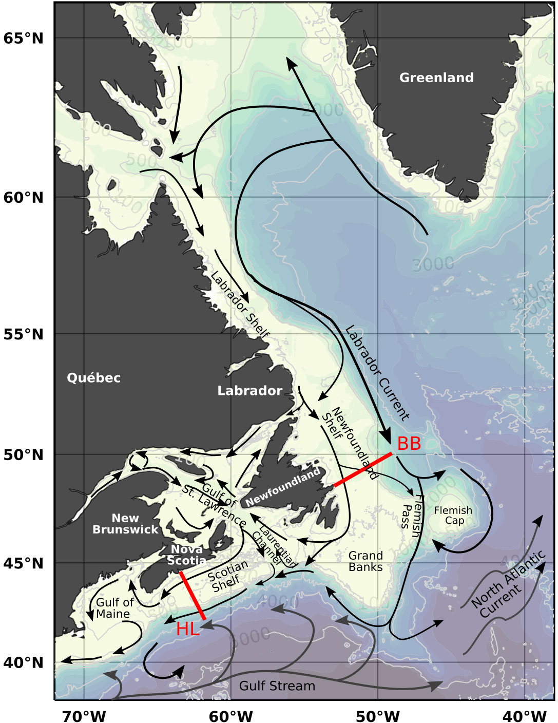
Figure 2 Map showing the Northwest Atlantic bottom topography (depth contour values in light gray) and schematic surface flow patterns (arrows). Black arrows are generally cold and fresher waters while the dark gray arrows represent warm and salty Gulf Stream and North Atlantic Current waters. DFO monitoring sections Bonavista Bay (BB) and Halifax Line (HL) are shown in red. Figure adapted from from Cyr and Galbraith (2021).

In addition to the regular occupation of the two AZMP sections, the acquisition of passive acoustic monitoring (PAM) payload for SeaExplorer and 4 Slocum G3 gliders in 2018 and 2022 has led to additional missions in Emerald Basin on the Scotian Shelf (close to the HL section) to monitor for marine mammal species, including baleen whales. The PAM missions include more experimental behavior than traditional glider approaches, including extended drifts at depth to minimize vehicle and flow noise for the acoustic recordings. The DFO Slocum glider PAM program is in the early stages, and not expected to be fully operational until late 2022/early 2023.

3 Regional oceanographic context for glider operations in Atlantic Canada

3.1 The Labrador Sea

The Labrador Sea is a crucial site for climate change-related research interests. The lack of reliable winter-time ship-based ocean observations has strengthened the approach of glider-based observations (de Young et al., 2020). Gliders have contributed high-resolution data to answer questions related to small-scale processes (Frajka-Williams et al., 2009), for example, mesoscale mixing and air-sea interaction (Frajka-Williams et al., 2014; Howatt et al., 2018). During the winter, glider surfacing periods need to be kept short to avoid damage to the glider from severe surface conditions or icing. Glider observations in this region began with Seaglider deployments by the University of Washington (Hátún et al., 2007; Eriksen and Rhines, 2008; Frajka-Williams et al., 2009) near Greenland. They continued with Labrador shelf deployments from Memorial as well as CEOTR.

A strong boundary current, the Labrador Current (LC) and West Greenland Current (WGC), bounds the Labrador Sea on its west and east (basin) sides, respectively (Talley and McCartney, 1982; Lab Sea Group, 1998). Deployments on the shelf needed to consider the strong currents (25–35 cm s^-1) as well as the steep topography that separates the shelf (200 m) from the deep ocean (3 km) over a short distance of only 30 km. Stratification in this region is less intense than in other parts of the Scotian and Newfoundland shelf. However, it can still exceed density differences of 2–3 kg m^-3 in the shelf zone requiring careful glider ballasting. Shelf deployments have been demanding and are restricted to the summer and fall due to sea ice and icebergs. The critical considerations for long winter deployments from an operational perspective focused on minimizing power consumption by using low power duty cycling of the onboard glider systems and decreasing the buoyancy drive of the glider. The Memorial-led deployments have successfully been carried out with long transit times to and from the sampling region, exceeding transit distances of 1500 km to reach the sampling site and to return. A key consideration was to optimize the glider transit path on the shelf to maximize the glider dive depth and reduce the number of buoyancy pump cycles – the main power draw on gliders. The battery budget for those legs did not exceed 25% of the total capacity making them feasible. A key strategy for the glider returning is to fly inside the LC and then near the Newfoundland shelf at the BB section, going with the coastal current into Trinity Bay. The average depth on this part of the Newfoundland shelf exceeds 300 m, allowing for better battery performance.

3.2 Newfoundland Shelf

On the Newfoundland shelf, section BB is located on the pathway of the southward flowing Labrador Coastal Current that originates from a mixture of Davis and Hudson straits waters (Figure 2; see also Florindo-López et al. (2020)). The characteristic sub-surface water mass (T<0°C, 50–150 m and 0–100 km in Figure 3) is generally referred to as the cold intermediate layer (CIL) (Petrie, 1988; Petrie et al., 1988; Cyr and Galbraith, 2021). The CIL is formed in the winter as a surface mixed layer that gets further insulated from the atmosphere at the onset of spring (see also Cyr et al. (2011)). On the NL shelf, the CIL is also characterized by high O₂ concentration levels and low Chl-a concentration (shown in Figure 3). Interestingly, the CIL on section BB is characterized by a relatively well-mixed core separated by two density interfaces above and below (squeezed isopycnals).

FIGURE 3

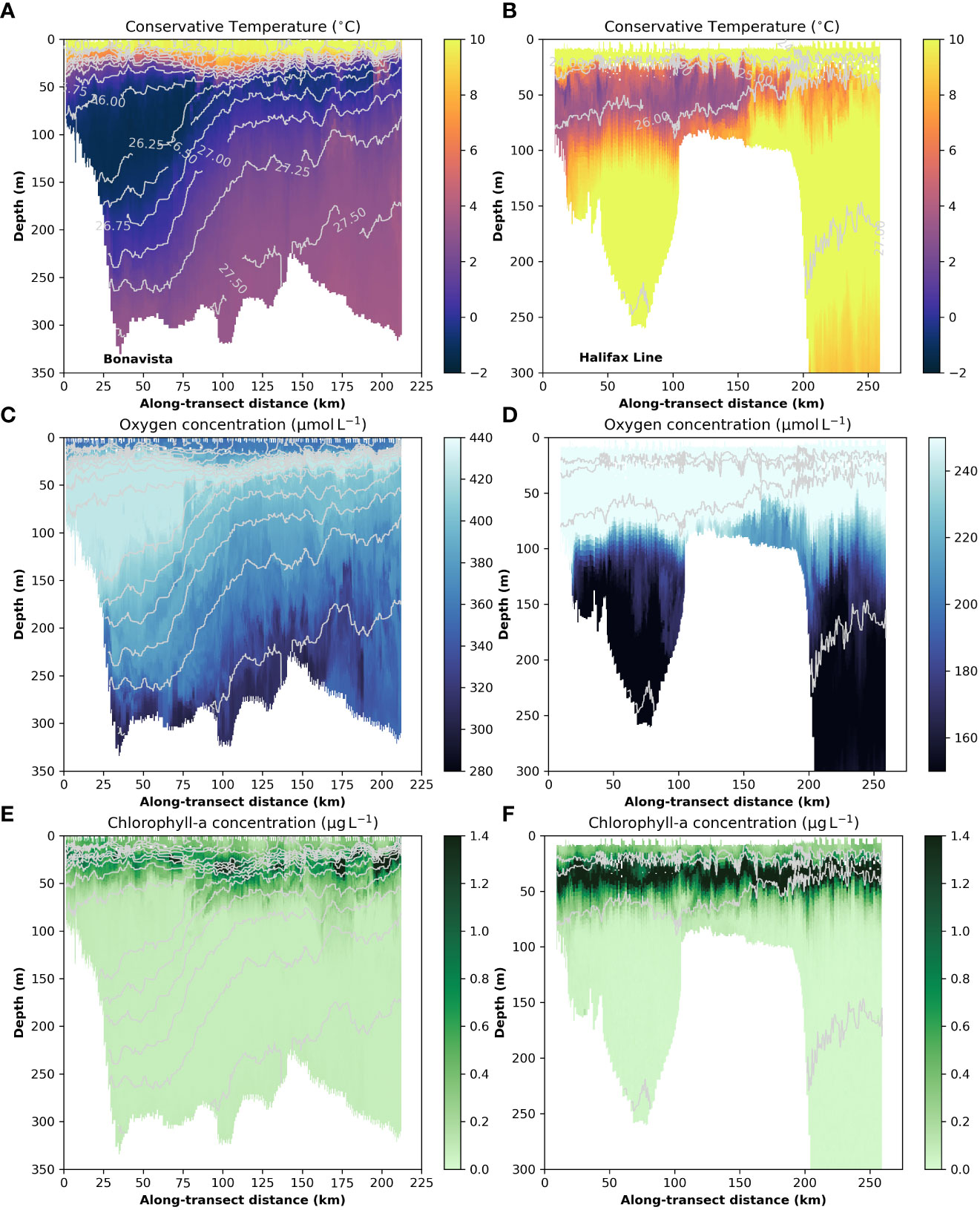
Figure 3 Contour plots of various variables measured by one DFO glider deployed on the Bonavista Bay section on the Newfoundland shelf during the summer of 2021 (21–30 July), left side, and on the Halifax Line on the Scotian Shelf during the summer of 2020 (16–26 July), right side. The plots are shown in function of depth and along-transect distance (see map Figure 2 for location). (A, B) Conservative temperature; (C, D) Dissolved oxygen concentration; (E, F) Chlorophyll-a concentration. Isopycnals are plotted in each panel with thin solid light gray lines (values identified in panels A, B). The conservative temperatures were calculated using the TEOS-10 toolbox (McDougall and Barker, 2011). For the oxygen and chlorophyll-a concentrations the manufacturer calibrations were used.

Further offshore (beyond 150 km), the main branch of the Labrador Current flows southward along the shelf break (Florindo-López et al., 2020). These currents carry subpolar waters from the Western Greenland Currents, which have undergone modifications in the northern Labrador Sea (Figure 2). Due to battery limitation, this branch of the Labrador Current is currently not systematically resolved by the glider monitoring program on section BB.

3.3 Scotian Shelf

On the Scotian Shelf, the section HL is located approximately halfway along the Nova Scotia coast and crosses both deeper basins (e.g., Emerald Basin) and the shallow outer shelf before transitioning to the outer continental slope into the open North Atlantic (Figure 2 for location). The hydrography of the Scotian Shelf is influenced by the upstream Labrador current and the Gulf of St. Lawrence outflow, which contributes cold and fresh (S ≤ 33) waters that extends to a depth of about 50–100m, as in Figure 3. The bathymetric connections to the deep North Atlantic and Gulf Stream-influenced water lead to an inflow of water off the shelf into the deeper basins creating highly stratified conditions in the near-coast environment. This environment is characterized by persistent warm water at depth below the CIL. Further away from the basins and the coastal currents, the outer shelf exhibits well-mixed conditions more typical of the offshore Gulf Stream-influenced waters. The sizeable lateral density gradients resulting from the freshwater outflow from the Gulf of St. Lawrence near the coast results in a persistent and dynamic coastal current, the Nova Scotia Current (NSC), which must be navigated at the start and end of all glider missions along the Halifax Line. The NSC varies seasonally, with the highest velocities of around 20 cm s${}^{-1}$ in the winter (Dever et al., 2016) and sometimes above 25 cm s${}^{-1}$. Currents on the shallow outer shelf are dominated by tides, while those along the shelf break/slope flow to the Southwest along the bathymetry. However, they are more likely to be impacted by mesoscale flow associated with the Gulf Stream and warm-core rings that propagate Northward and can impinge on the shelf (Smith and Petrie, 1982).

The gliders for the Scotian Shelf work must be capable of diving to a maximum depth greater than 250 m (Emerald Basin) but also be able to navigate in the shallower waters found closer to shore and on the outer banks (< 100 m). Due to limitations of the buoyancy engines in the original OTN G2 Slocum gliders (from 2011 to 2015), most of which were only rated to 200 m, the deepest portions of Emerald basin were not sampled, and the missions did not extend beyond the shelf break (usually stopping around station HL5). With the acquisition of the SeaExplorer gliders in 2017, rated to a maximum depth of 700m, whole depth sections across the HL are now possible, with offshore data down to the glider limit. The furthest extent reached is typically the HL7 station (42.475°N, 61.433°W), approximately 285 km offshore, with a total water depth of about 3 km. The limitation in going farther is due to battery capacity; significant power is consumed during the transit across the shelf due to the shallower water requiring more frequent dives. A typical HL mission (out and back) consists of approximately 1000 dives over about three weeks.

3.4 Gulf of St Lawrence

Most glider activities In the Gulf of St. Lawrence have been realized by UNB, Transport Canada and CEOTR (DAL), conducting acoustic whale monitoring since 2016. These missions focused primarily near the Shediac valley, East of the Magdalen Islands and, since 2021, the Laurentian channel shipping lanes. Parts of the Gulf of St. Lawrence serve as a migratory feeding ground for various whales, including the critically endangered North Atlantic Right Whale (NARW). With the digital acoustic monitoring DMON system (Baumgartner et al., 2013), specific baleen whale calls can be detected and classified on board the glider. These detections are returned to shore daily to an analyst who verifies the detections. Once verified, they are submitted to DFO and Transport Canada for monitoring and management. Transport Canada uses these acoustic detections of the NARW alongside their visual surveys to trigger speed restrictions in parts of the Gulf of St. Lawrence shipping lane (Figure 4).

FIGURE 4

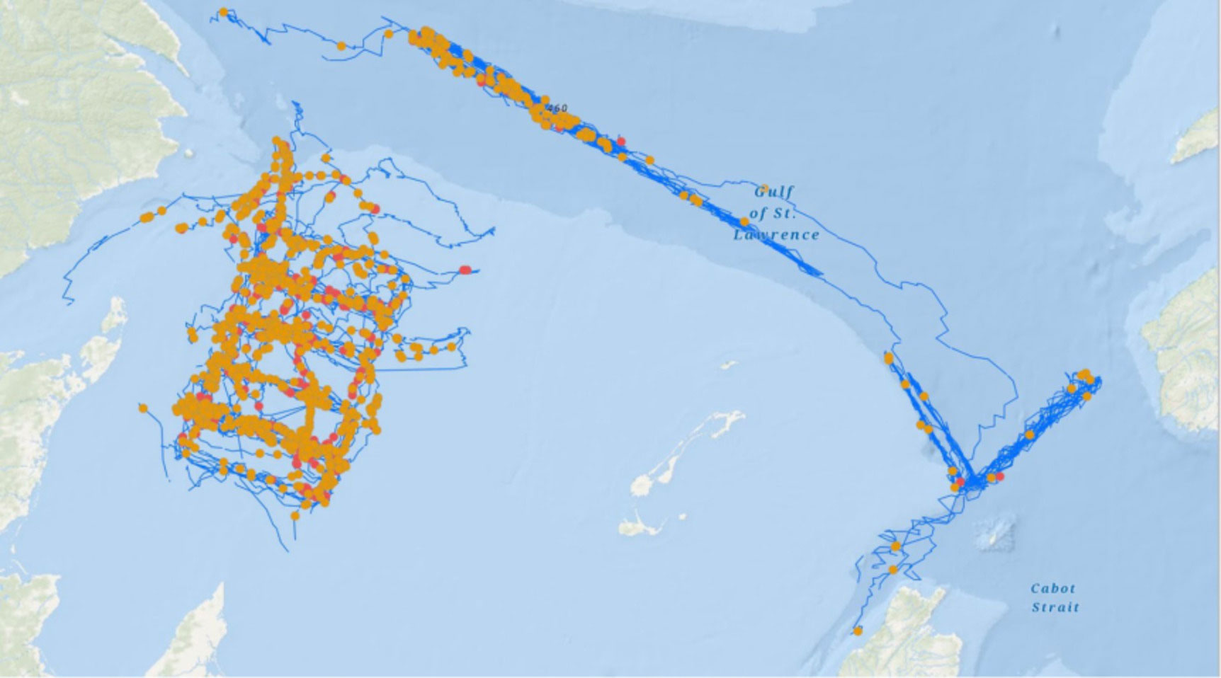
Figure 4 Example figure showing CEOTR Acoustic Whale monitoring in the Gulf of St. Lawrence since 2016 with possible detections in orange and validated definite detections of North Atlantic Right Whales in red. (Credit DFO, https://gisp.dfo-mpo.gc.ca/apps/WhaleInsight/eng/?locale=en).

Parts of the southern Gulf of St. Lawrence pose challenging operational considerations, including shallow depths of less than 50m, strong tidal and persistent currents exceeding 25 cm s ${}^{-1}$, and strong stratification with near surface densities as low as 1017 kg m ${}^{-3}$ and bottom density of 1024 kg m ${}^{-3}$ and denser reaching in situ density of over 1029 kg m ${}^{-3}$ at depths exceeding 150 m. This makes operating shallow gliders a real challenge as the density range to overcome is very substantial (exceeding ± 4kg m⁻³).

Some missions have taken place in deeper waters (400–500m) towards the Laurentian Channel and Cabot Strait North and South-West of Orphan Bank, where stratification is reduced. A CIL spans from 50 to 150 m in depth, with an approximately homogeneous density of around 1024 kg m${}^{-3}$, T<1°C (Banks, 1966). Below the CIL, the water column is continuously stratified to the bottom and made up of a mixture of Labrador Current and salty North-Atlantic water. In this bottom water, scientists have observed a continuous decline in O${}_2$ with pronounced seasonal hypoxia (O${}_2$ saturation $<$ 40%) in most of the Gulf at depths over 250m during late summer (Gilbert et al., 2005; Jutras et al., 2020). In some parts like the Cabot Strait, hypoxia can be observed year-round. Similarly, pH levels have decreased, but measurements are not as comprehensive. More recently, Memorial has been operating gliders in the Northern Gulf, going from Bonne Bay into and across the Esquiman channel to observe seasonal variability of O${}_2$ levels in bottom waters.

4 Lessons learned: operating gliders in Atlantic Canada

4.1 Understanding mission costs and benefits

Gliders can provide data that is not attainable by other platforms for similar costs. Gliders can complement other monitoring programs such as traditional ship-based and mooring-based monitoring. Use-cases of continuous glider monitoring along traditional ship-based surveys, can help uncover spatial and temporal patterns that are not visible in the synoptic snapshot of a quarterly or semiannual ship cruise. Glider-based sampling efforts should be organized as long-term sustained glider operations (Liblik et al., 2016; Weller et al., 2019) to add value to an existing monitoring program however. Given their relatively low cost and high spatial sampling resolution, they provide a significant cost reduction on a per profile comparison with ship-based surveys. For comparable roles, gliders are an order of magnitude less costly per profile (Testor et al., 2019). Their availability, compared to research ships in Atlantic Canada (Hughes, 2019), means gliders, are one of the most cost-effective methods presently available to fill and complement ocean observing gaps.

Three points drive the costs for sustained glider operations: (1) How many months of glider data are needed per year to cover costs? (2) How many gliders are needed/available? (3) What logistics are required for deployments? To explain point (1), we note that the amount of data collected per year is driven by the objective of the program. However, to sustain a glider program requires enough glider-activity to justify the glider infrastructure and cover operating expenses. For example, if a project requires five six-month glider missions per year, this means that the staff, equipment and logistics can be worked out to support this need. Another challenge is the fact that short and long missions have similar up-front labor and logistical costs. This means that for the same amount of funding available, organizing a smaller number of longer endurance missions is more cost efficient than meeting the same research requirements with many shorter deployments. This is because a 6-month mission is not, simply six-times the cost of a one-month mission (see Table 2). We note that costs summarized in Table 2 are only the basic direct operating costs and importantly do not include institutional overhead costs which can increase costs by more than 50–60% in some cases. The second point is about the number of platforms deployed and the number of gliders available. If a region needs monitoring at all times, this program will require more gliders and be more expensive to sustain, than one which only needs six-month of data coverage. Another important aspect not considered here is the obsolescence and end of life of gliders. This point is different from losing gliders and needing to replace them, but can have a big impact on glider operations and support of equipment. In the case of Slocum gliders the older glider versions G1 and G2, still used in Atlantic Canada, are no longer fully supported by the manufacturer, meaning that these vehicles will eventually need to be phased out due to a lack of replacement parts. Some groups factor equipment depreciation into their operating costs to deal with the need to replace equipment even if it is no strictly lost or damaged during regular operations. It would not be unreasonable to assume a 10–15 year end of life span for new gliders purchased today. These equipment life spans should factor into incremental costs of glider missions to ensure equipment can be replaced before becoming obsolete. The third significant factor determining running costs are those of the logistics involved in deploying and recovering gliders. A program that is dependent on large vessels for deployment, due to remoteness or to maximize endurance, will be much pricier than one which can be launched near shore. We summarized these aspects in Table 2, highlighting costs among major categories. Another aspect we implied in the costs of (1), (2) and (3) above are related to the calibration requirements. Annual calibrations of sensors (e.g. CTD) will require stand-by equipment or lead to down-time in sensors. If reference data are required for validation then this too will increase cost (3).

TABLE 2

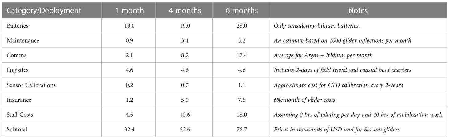
Table 2 Slocum glider deployment costs.

4.2 Glider mission planning

4.2.1 Coastal, shelf vs. deep ocean

Working in the coastal ocean is typically the riskiest of all operational zones given possible collision from ships (Merckelbach, 2013) and strong currents leading to increased workload for glider pilots. Deployments of gliders in coastal waters typically require monitoring 24/7. This is due to the shallow depths (< 100 m), the concentration of fishing activity, ship traffic and stronger currents. In addition, from winter to early spring, much of the Gulf and Newfoundland shelf is covered with sea ice, making glider work nearly impossible. Strong coastal currents pose a real challenge. In shallow water, the glider will spend only a short time diving (8–15 min) between inflections at its design speed, travelling only a short distance (90–150 m). A glider doing 100 m dives with a vertical speed of 12 and horizontal speed of 25 cm s ${}^{-1}$ in an area with no currents should typically progress 400 m in the horizontal during a single yo. With a 15 cm s ${}^{-1}$ head-on current, this distance could be easily reduced to only 160 m, resulting in slower progress. If the currents are stronger, the glider could be swept towards the coast, quickly reaching the minimum practical dive depth (30 m for 200 m & 1000 m gliders). While some groups operate gliders configured for dives shallower than 30 m (30 m pump), such gliders are currently not employed in Atlantic Canada; hence, work in areas shallower than 30 m is not routinely done.

Most Atlantic Canadian glider operations are on the shelf, focusing on repeat observations along established hydrographic lines (DFO) or monitoring certain regions (CEOTR, Memorial). The shelf topography increases gradually (100 m over 200 km) with average depths around 200–300 m. Due to strong tidal currents in Atlantic Canada, particularly in the Gulf of St. Lawrence and Scotian Shelf, these missions require planning to ensure gliders maintain position or reach their target stations. Gliders owing to their near neutrally buoyant design and slow speed, are strongly affected by ocean currents.

Another challenge in operating gliders on the shelf is that gliders are not optimally efficient in diving in depths less than their design depth. If the glider is designed to work in 1000 m, doing 200 m dives can be as much as five times less efficient for the same distance travelled. If the glider is transiting the shelf to reach the open ocean, the battery budget on the shelf should be minimized to increase endurance at the target site. CEOTR and Memorial groups have been utilizing thrusters on gliders to speed up or overcome strong currents near the shelf and speed up the glider’s journey towards the target area. For example, Figure 5 shows a thruster-assisted crossing of the Labrador Shelf to speed up the transit time of the glider from the deployment site near Cartwright on the shelf to the open ocean. The glider deployed in 100–200 m deep water used the thruster until reaching 300 m deep water and resumed flying regular yo’s (1-yo is a glider dive and climb cycle). The time spent in shallow water in strong currents was thus minimized, decreasing glider advection in strong southward flowing currents and inefficient use of the buoyancy engine. The CEOTR glider group minimizes thruster usage to collect high-quality acoustic data. However, it is occasionally used to help navigate against nearshore currents encountered during recovery.

FIGURE 5

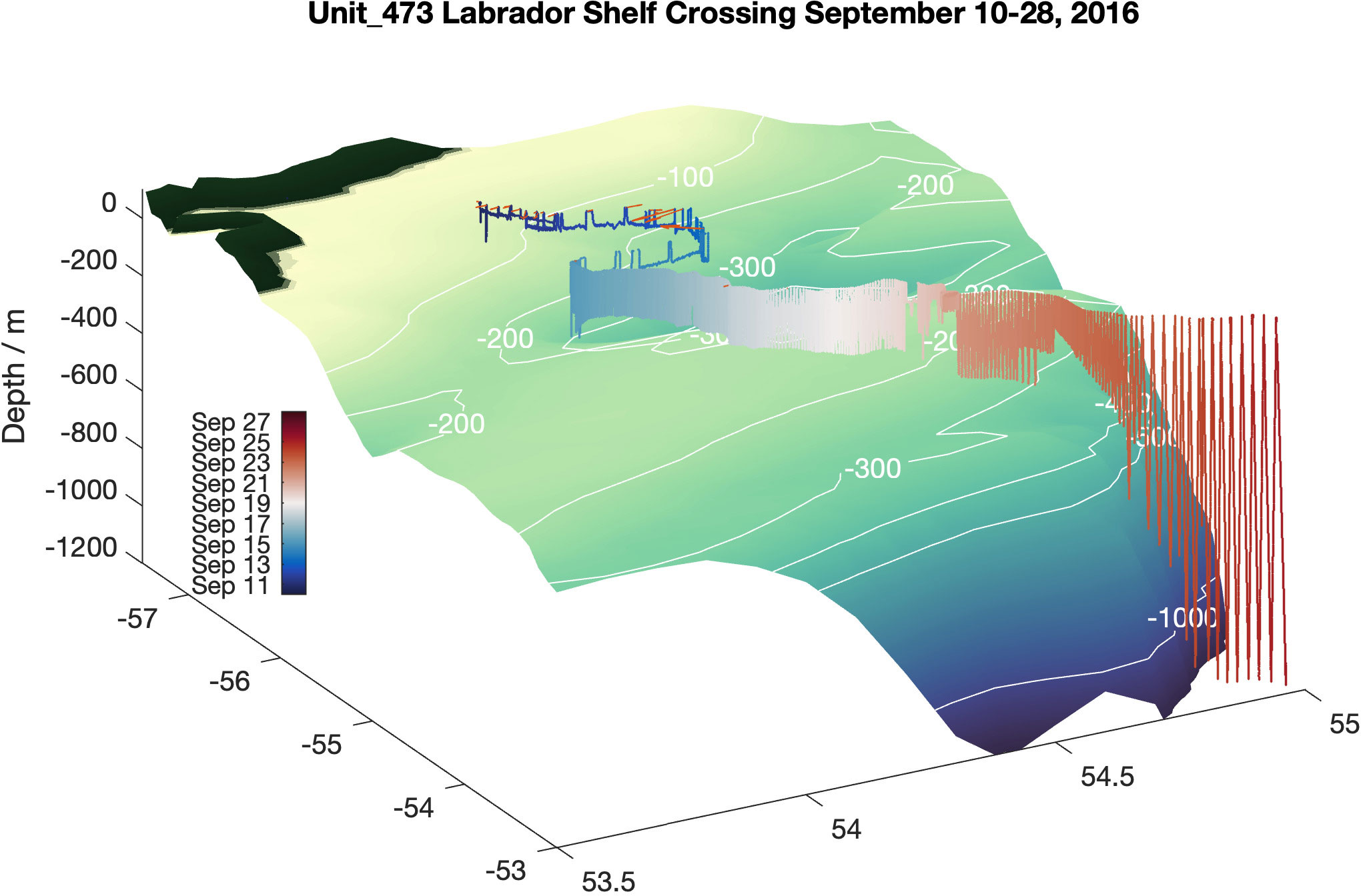
Figure 5 Glider track (unit 473) crossing the Labrador Shelf deployed near Cartwright on September 10, 2016. The colorbar indicates the time of the glider travel going from blue (start) to red (end) of the transect. The glider first used a thruster at depth to cross strong shelf break current. Once in deeper waters the glider resumes flying regular yo’s (1 yo = 1 glider dive/climb cycle). Depth contours are indicated in white.

At the shelf break, topography increases rapidly (3 km over 10 km). In Atlantic Canada, the glider operations near the shelf break and the deep ocean operations merit special consideration. The more extreme weather conditions (winds up to 120 km hr ${}^{-1}$, 20 m waves, spray ice, icebergs) result in potentially less frequent communication (data uploads) and potentially more difficult deployment and recovery. The lack of ships and good weather makes glider emergency recovery more difficult and missions riskier. On the other hand, deep water operations are less challenging to manage from a piloting point of view given that the glider surfaces less often, is diving and moving forward more efficiently. Positional accuracy is usually less of a concern given the larger scales of ocean processes. For example, the Memorial led Labrador Sea missions last 4–7 months, with the glider spending most of the time in deep water (>3000 m), with mean currents near 0.1 m s${}^{-1}$. The gliders spend less than 15 min each day at the surface, meaning the work of pilots checking on the glider is reduced. For winter operations, ice movement should be considered. Ice edge maps are reviewed and considered during mission planning for the Memorial Labrador Sea missions. Ship traffic in the deep ocean is sparse and not usually a concern.

4.2.2 Weather

In Atlantic Canada, suitable glider weather windows can take weeks to develop. While getting a glider into the water is straightforward, recovery can be challenging if there are problems and weather conditions are poor. Ideally, no launch should occur from a small boat in strong to gale force winds. It is sensible to practice the procedures in sheltered areas before attempting to maneuver a glider in and out of the boat in the open ocean for the first time. Having a detailed checklist to help through a potentially tricky deployment or recovery is helpful. Having onshore support can also significantly help as they can provide communication and control the glider from the quiet of the lab. There is more flexibility on a large vessel, and a deployment can take place up to sea-state 4/Beaufort Scale 5 (wind 30–38 km hr ${}^{-1}$, waves 1.5–2.5 m), if necessary.

In judging the weather window, it is better to launch a glider under the right conditions rather than precisely on target. Gliders can travel 25–40 km per day. A hundred km is therefore at most a loss of four sampling days, which is not always critical to the mission’s overall success, likewise for recovery.

4.2.3 Data sampling

One of the main requirements for oceanographic glider sampling in Atlantic Canada is to resolve shelf and upper open ocean processes. The glider’s performance (mean maximum speed without thruster 0.27 m s ${}^{-1}$) must be respected in the choices of the glider’s mission. This has important implications for how the glider is flown. If resolving the spatial structure is essential, then a glider can be sped up relative to a glider that needs to sample the entire water column but not as often. For example, mission design should consider the cutoff for time, space and depth scales for the data to be collected. An illustrative example is chlorophyll on missions where the glider is diving below the euphotic zone (deep ocean). In the central Labrador Sea, chlorophyll signals are concentrated in the upper 400 m. Hence vertical sampling of chlorophyll could focus on depths down to 400 m. In order to conserve power, the sensor could be switched off below this depth. If the objective is to provide maximum horizontal resolution of chlorophyll along the glider flight path, then the maximum dive depth of the glider could be adjusted to provide more frequent vertical profiles in the layer. This could also apply to other ocean features. For example, if the objective is to measure frontal processes, like a boundary current, one would need to increase the horizontal speed of the glider, for example with a thruster, to improve the ability of the glider to navigate in the environment. Faster horizontal and vertical glider speeds are also important because in fast moving oceanic environments such as the boundary current, spatial and time scales are shorter compared to the open ocean requiring frequent vertical profiles to resolve ocean signals. The cutoff frequency for ocean signals will be dictated by the horizontal distance and temporal separation between profiles and the vertical data resolution. In the Memorial-led Labrador Sea missions, a thruster was used to repeatedly zig-zag across the Labrador Current at horizontal speeds of up to 50 cm s ${}^{-1}$, reducing advection, allowing sufficient resolution to resolve eddy and Ekman transport of heat, oxygen and salt (Howatt et al., 2018).

Another consideration for planning glider missions are data quality control procedures. Glider sensors generally require specific post-processing to achieve data quality like ship-based casts. In general optimal performance of optical sensors such as optodes and CTDs have a dynamic component as well, dependent on the vertical velocity of the glider. For best data processing results and quality, the dive and climb speeds should be kept constant to improve response time corrections of the data. Using the auto-ballast feature on Slocum gliders, significantly improves the consistency of vertical glider dive/climb speeds. For Memorial and CEOTR gliders, generally unassisted vertical glider speeds are between 6-15 cm s^-1. Some known glider sensors, such as oxygen optodes, suffer from drift. If high-accuracy O₂ data are essential to the mission, strategies for quality assurance should be built into the mission, for example, by designing the mission around other observing programs. In the case of DFO BOON missions, the glider tracks follow established hydrographic sections from DFO AZMP; hence, glider data can be compared/referenced to ship-based data. For oxygen optodes, it is also possible to arrange the sensor on the glider to allow in-air calibration and drift corrections (Bittig and Körtzinger, 2015; Nicholson and Feen, 2017) employed in recent Memorial Labrador Sea Slocum glider missions. These considerations could alter the sampling of the glider. In the case of optode drift corrections, the glider needs to spend time sampling in the air at the surface.

4.3 Power management

Battery power management is a crucial concern for the endurance of missions, particularly for deployments of long duration or for vehicles carrying multiple sensors. There are four critical choices users can make related to glider endurance:

• The frequency at which the ballast pump is used (deep vs. shallow dives),

• The amount of buoyancy used (how long the pump is running to change the glider apogee)

• Payload settings and drag (how many sensors are being sampled and how often, how streamlined is the glider)

• Surface communications (how long the glider is transmitting/receiving data when not in a mission)

Related to these choices are several strategies for conserving power before deployment and once a glider is in the water.

4.3.1 Before deployment

4.3.1.1 Ballasting

Adjusting the glider buoyancy to match the density range encountered in the deployment region is the key attribute that allows the glider to dive efficiently inside the envelope provided by the buoyancy engine. Once a glider is deployed, the ballasting is fixed for the mission until recovered. Hence proper ballasting is key before deployment so that the glider is efficiently diving. The glider should be ballasted to maintain a consistent dive/climb speed. The glider buoyancy engine displacement needs to be taken into consideration. Most Atlantic Canada missions are ballasted for a mean surface density of 1025 kg m^-3 based on a surface density of 1023 kg m^-3. and a density of around 1029 kg m^-3 near the maximum dive depth of 500 m on the Atlantic Canadian shelf. Glider users must consider the specific range of seawater density at the surface and the maximum dive depth for every glider deployment to ensure the glider is properly ballasted for the intended deployment region.

4.3.1.2 Payload settings

It can be advantageous for mission endurance to set some sensors to lower sampling frequencies before deployment if this is not possible within a mission and if high sampling resolution is not required. Careful consideration must be given if the sampling rates and other sensor payload settings match the data requirements for the mission objectives. The glider may also have restrictions on the maximum sampling frequency it can support. Some sensors, for this reason, log data internally, with the glider only recording a subset or derivative product of the data (e.g. AZFP or JASCO Observer). For Slocum gliders, if power conservation is necessary, it may not be easily possible to adjust the sampling frequency of the sensors while deployed on a mission. This is because the Slocum glider lacks a setting for sampling frequency and provides continuous power to the sensors when sampling is turned on. Changing sensor sampling rates would require changing settings on the sensor side, which can be made difficult by bad weather and risky if incorrect sensor settings can corrupt data quality. SeaExplorers can adjust the sampling settings of sensors while deployed at sea.

Pilots can help reduce power consumption from sensors by choosing depths at which to sample or by choosing to sample only certain dive/climb cycle intervals. Sampling can be adjusted so that only up profiles are sampled, or perhaps only sampling every two yo’s.

4.3.1.3 Drag

Gliders are optimized for efficiency and endurance at slow (10-30 cm s^-1) speeds relative to powered AUVs (50-100 cm s^-1). As much as possible, sensors and components should be integrated into the vehicle hull or streamlined to reduce drag, which would cause slower progress resulting in more inflections for the same distance travelled for a streamlined glider.

Biofouling in long missions can increase drag, deteriorate glider speed and dive/climb performance. In the worst case, the glider could stall. Atlantic Canadian waters below the thermocline tend to be frigid; hence, they are not as affected as missions ofthe same duration in tropical regions. Minimizing time at the surface can decrease impact of biological growth when of concern.

4.3.2 During a mission

4.3.2.1 Buoyancy drive

The buoyancy engine is the component on a glider that uses the most power. Some gliders can determine the buoyancy needed to achieve a targeted speed - a feature called automatic ballast. A glider with less total displacement must pump less water/oil to inflect and save power. The dominant current draw occurs at depth when the glider engages the pump to push water. The buoyancy engine will draw between 2–6 A and run for 30 s or more to push out 264 cc’s (1 cc=1 cm³) of water (numbers from a G2 Slocum low displacement 1000m pump). The same glider will also be more efficient if the glider needs to push out less water on the climbing cycle than during the dive. It is also true, however, that at greater depths, the relative power consumption of the pump will increase (Figure 6). Hence there are many reasons to minimize the drive required for successful dives/climbs, and the rate of dives and climbs should be minimized.

FIGURE 6

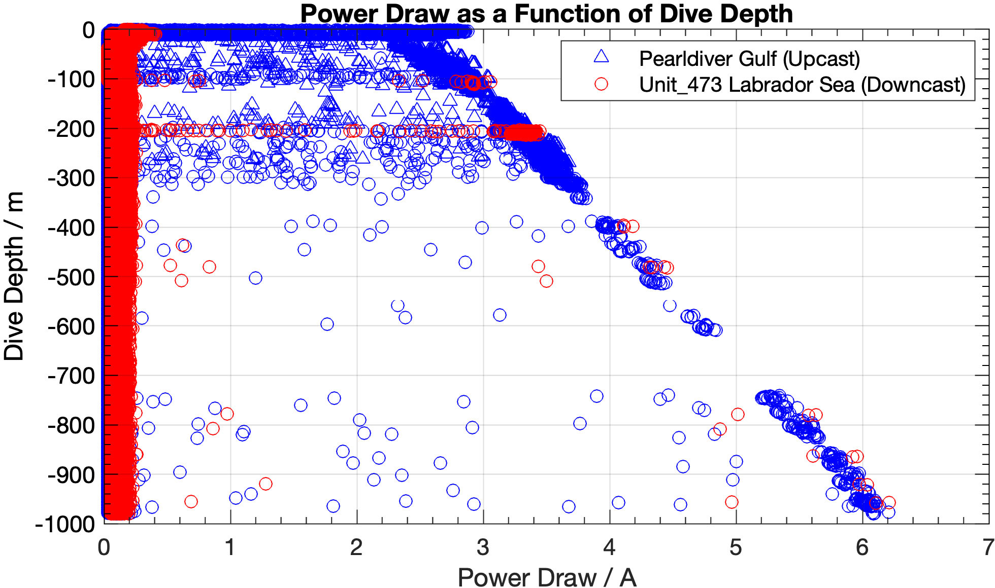
Figure 6 Figure shows the power consumption as a function of dive depth for a G2 glider with the low displacement oil pump (± 264 cm ^-3). Blue markers are upcasts and red are downcasts. The downcast has a lower power draw during inflections, compared with upcasts. Triangles are from a Slocum glider deployed in the Gulf with more variable dive depth and variable power consumption during climbs. Circles are a glider deployed in the open ocean in the Labrador Sea with dive depths reaching 1000 m.

A slow diving/climbing glider will have greater endurance. However, the glider needs to be ballasted well enough to be within the range of the buoyancy engine - see point above (before deployment). For the CEOTR and Memorial Slocum glider missions, automatic ballasting maintains even dive/climb speeds of around 10–15 cm s^-1. In open ocean conditions with deep dives, as little as 300 cc’s can be used (Labrador Sea missions). Endurance of upwards of 7–months is routine for the Labrador Sea missions. For coastal missions and those in the Gulf, more buoyancy (400–500 cc) is needed to overcome the vertical density gradient caused by fresh surface water. Using more/less buoyancy will also speed up/slow down a glider.

4.3.2.2 Surface communications

Gliders at the surface communicate via the Iridium modem. After the buoyancy engine, this is the most energy intense element of the glider dive/climb communication cycle. Operators typically set gliders to the surface and communicate at regular intervals or when completing X–number of yo’s. The longer time between yo’s, the better the energy consumption, but the less frequent a GPS fix will be available to validate the glider’s location. The CEOTR/Memorial/DFO glider missions tend to operate in shelf areas based on timeouts to communicate every 3–6 hours (depending on location), whereas, in deep water, the CEOTR/MUN gliders are set to complete two or more yo’s (approx. 8–11 hours). When at the surface, the glider can send back snapshots of data. Depending on requirements for endurance, this snapshot can be kept minimal, and surface times can be reduced to less than 15 min per day for open ocean deployments with some data downloads. The less time a glider spends at the surface, the better for the battery power and less risk from surface action (waves, wind, ships and ice).

4.3.2.3 Duty cycling

Gliders usually have two computers: a flight computer that handles the navigation and a payload computer for sampling data from science sensors. On Slocum gliders, the flight and payload computers can be duty cycled when not in use, saving power. For flight mode, this happens when the glider is diving/climbing, the motors and actuators are not moving, and the altimeter is not returning positive hits. The user can set the sleep periods for the glider flight computer.

4.4 Glider operations

4.4.1 Launch and recovery

Launch and recovery is likely the shortest and most crucial component of the overall success of the glider mission. Gliders are somewhat fragile: wings can break, hulls can crack, causing leaks, or sensors can break. Therefore deployment/recovery needs to occur in as low as possible sea states (ideally wind < 10 km h^-1, waves < 1 m). Deploying a glider is the easiest part. Recovery tends to be more challenging. We recommend never deploying a glider in weather that prevents recovery should it be necessary. We will discuss small vs large vessel launch/recovery options and how to organize remote deployments.

4.4.1.1 Small vessel

Ideally, glider launch and recovery are done by a small vessel with a low freeboard, such as a Rigid-Hull Inflatable Raft (RHIB), sliding the glider via a cart or cradle (see Figures 7A, D for Slocum and SeaExplorer launch; and Figure 8B for Slocum recovery). Most gliders deployed on missions in Atlantic Canada are launched from a small speed boat or fishing boat within 20 km of the coast. When operating in uncertain ocean conditions, e.g., nearshore where there may be fresher surface water or given uncertain glider ballasting, gliders are usually deployed with a safety buoy. The safety buoy allows the retrieval of the glider in case it does not come back to the surface by itself. After the first test dives, gliders sometimes need to have their external ballasting adjusted on site.

FIGURE 7

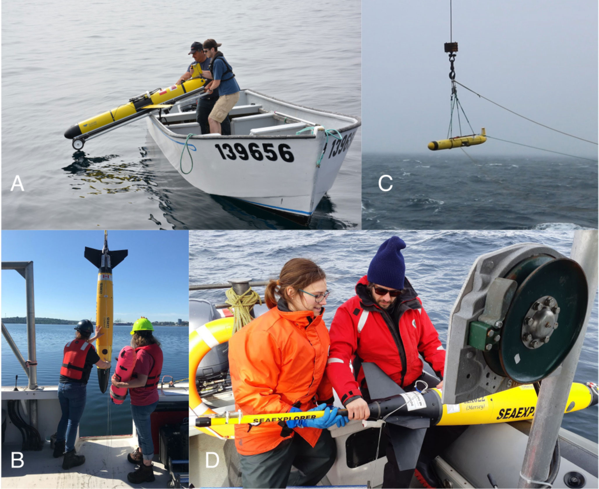
Figure 7 Examples of common launch options for underwater gliders (A) Slocum glider with top mounted sensors launched via cart; (B) via a release mechanism from a ship crane; (C) SeaExplorer glider launched from a ship crane; and (D) launched over the side of an FRC.

FIGURE 8

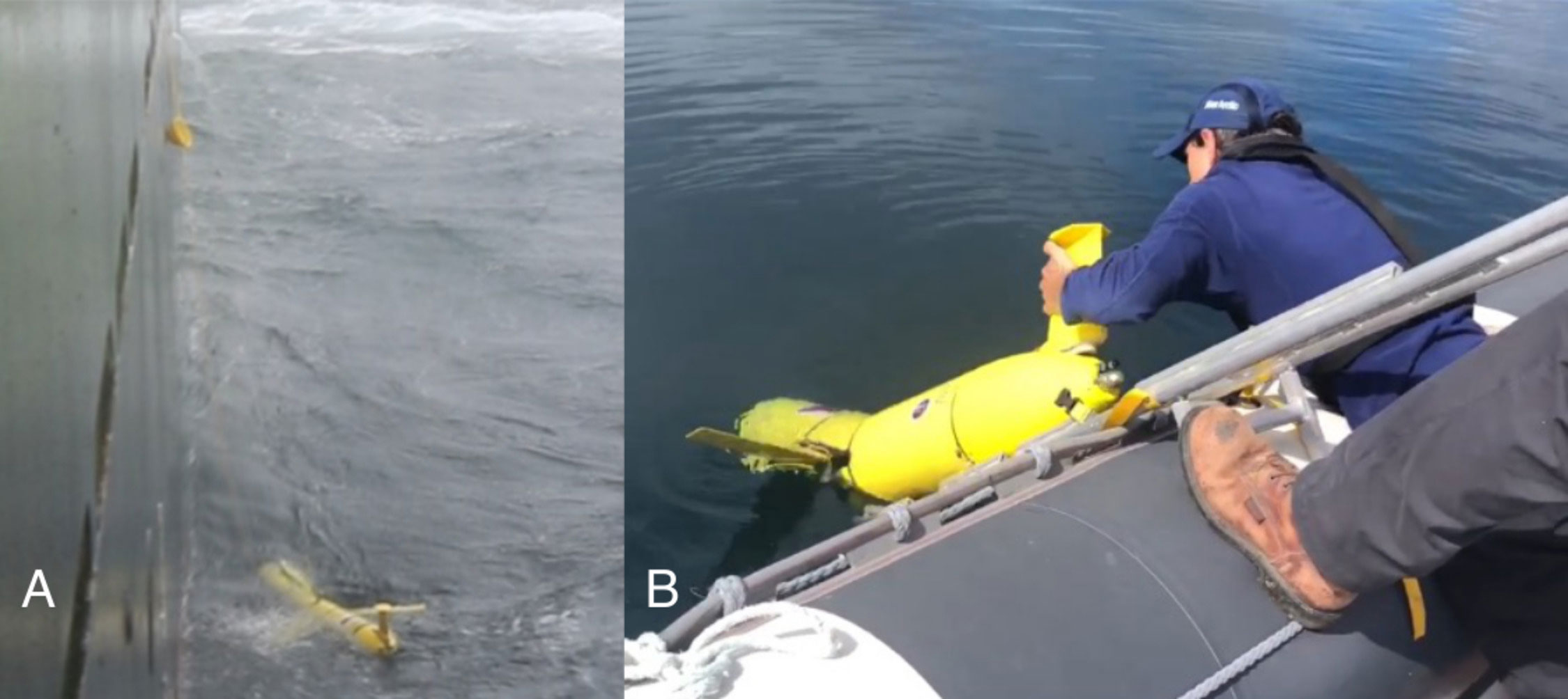
Figure 8 Examples of recovery options for gliders (A) Slocum glider nose recovery mechanism with a glider in trouble due to fin malfunction; (B) normal Slocum glider “calm weather” recovery using a cart over the side of an FRC.

4.4.1.2 Large vessel

Easy access to the glider during deployment is essential and not simple from a large ship. If working on a large vessel and if it’s possible, it would be best to launch a smaller vessel such as an FRC from which to deploy the glider. Launching the glider from a large vessel typically requires using a crane (see Figure 7B) for crane launch). Crane launches require special rigging, often custom-made and manufactured in-house by the glider groups (see Figure 7C). Sometimes, the vessel may be equipped with a mechanism on board to pick up the glider and release it without damage. Recovering/deploying gliders with a drop net is not advisable as sensors can be tangled up, the wings or the antenna can break and more. Some gliders have a built in recovery mechanism (see Figure 8A) for Slocum example) that can be triggered remotely by the pilot to release a recovery line which the ship crane operator can use to pull the glider up on deck.

Using vessel glider launch/recovery rigging should be a well-planned exercise with lots of practice on land to ensure all rigging used works well. Ideally, this takes place from a small craft with a low freeboard so that the glider can be held and guided onto the boat. If recovery is from a larger vessel, it is vital that the rigging used is well tested for the procedure. During recovery, a collision between vessel and glider is harder to control, given the communication lag between the deck and the bridge. Sea states offshore are often more limiting, making it harder to control the glider as it is picked up from the water. No matter the vessel, having a skilled operator and established communication with the crew is essential. For example, having protocols for maneuvering the ship in water during and after launch is necessary to ensure the glider does not collide with the sides of the boat or the propeller. Clear signals should be used, and the step-by-step plan for launch or recovery should be discussed with all field personnel, including the captain and crew.

4.4.1.3 Remote deployments

Typically, gliders are deployed by dedicated technical staff in a reasonably controlled environment. It is also possible to deploy and recover gliders remotely if an adequate plan is in place. CEOTR routinely ships gliders to Northern Labrador and has established procedures with the community and boat captains. All the usual deployment considerations should be made with the addition of a training session with the vessel crew. Care should be given to: a pre-deployment briefing with the crew, glider systems assessment from the glider technicians before the scheduled deployment, the establishment of a communication protocol between the ship and the glider crew (i.e., iridium phone, VHF or other), demonstration of locations suitable for handling, laminated instructions and spares (i.e., wings, wing rails, ballasting weights, power plugs, recovery and launching hardware) sent with the glider, and a plan for return shipping, with considerations for lithium batteries, if present.

4.4.2 Glider piloting

Glider piloting requires operating the vehicle in the water by maintaining positioning control and ensuring data gets collected. Operating gliders has become more routine, but knowing how to troubleshoot a glider remains an essential aspect of piloting. In general, glider piloting is a 24–7 responsibility for trained personnel, but in practice, on call periods are delegated to pilots on duty, receiving text and email alerts to prompt actions by the pilot. Vehicle manufacturers usually provide training sessions for new users. Experienced glider groups may have additional training opportunities through experienced staff. In Atlantic Canada, CEOTR has provided Slocum glider training for new glider users after receiving basic training from Teledyne. DFO staff have trained CEOTR and Memorial staff on SeaExplorer’s. The pilot relies on servers to communicate with the glider. Memorial and CEOTR share and use each other’s Slocum glider server infrastructure in case of downtime or for any other reason. SeaExplorer uses the Alseamar GLIMPSE environment, which the manufacturer maintains.

The time spent piloting a vehicle depends on the area of operation (mission objective), the experience of the pilots (training & prior piloting), the behavior of the vehicle (equipment issues) and access to data to assess and adapt the mission plan (piloting tools). For example, coastal and shelf operations are more demanding on daily piloting time (2–3 hours per day) due to more frequent communication windows and more emphasis on controlling the vehicle’s position due to ship traffic, stronger currents and steeper topography. For coastal and shelf missions, one requires access to accurate, up-to-date bathymetry charts and access to a tool that overlays glider position and bathymetry when in coastal zones. In recent years, CEOTR, Memorial and DFO have worked with a path-planning system (https://www.oceangns.com/) for optimal glider routing based on current forecasts (von Oppeln-Bronikowski et al., 2021b). For example, Environment Canada provides the Regional Ice Ocean Prediction System (RIOPS) Model (Smith et al., 2013), which provides 48-hr. forecasts in Atlantic Canada. OceanGNS can take these and other ocean model forecasts [e.g. HYCOM (Chassignet et al., 2007)] and predict the optimal path, minimizing head-on currents and assisting glider mission planning and operations. An example route plan (Figure 9) shows a glider track inside the OceanGNS portal and route planning used to find the best path for the glider in the boundary current.

FIGURE 9

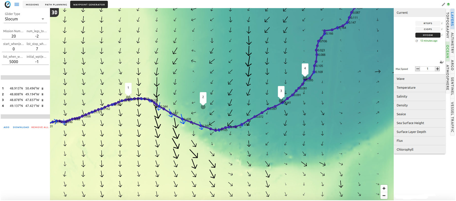
Figure 9 Example of mission planning and piloting viewed in the OceanGNS portal (blue arrows are glider depth averaged currents, black are model depth averaged currents, magenta line is the glider track, black circles are waypoints). Waypoints and corresponding glider tracks are shown. As the glider enters the strong current regime (waypoints 1 and 2), the ability of the glider to meet the targets is reduced and new waypoints must be given (waypoints 3 and 4) which are further offshore and orient the glider 90° to the current to avoid inefficient glider flight behavior.

In Atlantic Canada, some regions of the Newfoundland shelf have poor bathymetry maps (for example, Trinity Bay). One of the significant challenges operating gliders on the Atlantic Canadian shelf in the winter is the dynamic ice situation. For Memorial and CEOTR’s winter operations, Environment Canada ice charts and OceanGNS are used to adapt the glider mission to the ice situation. In addition, Automatic Identification System (AIS) traffic is monitored from sources such as https://www.marinetraffic.com/ to avoid a collision or getting gliders tangled up in nets. Open ocean missions typically require less active intervention, sometimes with as little as 30 min day (Memorial Labrador Sea missions). Windows for correcting the glider path or changing sampling are fewer, meaning mistakes or changes can take up to a day to take effect. Some points to keep in mind for piloting are as follows:

• Ship traffic: Knowledge or access to AIS data to avoid collision is critical. In certain areas, fishing boats do not have AIS transmitters and knowledge about their patterns and when and how they fish can help minimize problems.

• Power consumption: Understanding the glider’s battery consumption and projection for how long the glider can stay deployed to make informed decisions on when to recover the glider or initiate a home-bound leg.

• Backup server: Glider server to communicate with the glider in case the main service fails (e.g., SFMC for Slocum’s), for example, during a power outage affecting the institution carrying out the deployment. This backup could exist as a cloud server or another glider group in a different location (Memorial and CEOTR).

• Currents and Bathymetry: When reacting to currents/slower glider progress, it is essential to remember that it takes time for the glider to progress. When the water is relatively shallow, such as on the Scotian shelf, multiple dives mode (between 5 to 10 successive dives) is one way of progressing. Accurate marine charts and topographic models are crucial to avoiding shallow spots that slow gliders down.

• Weather: A reliable source for offshore weather and ocean conditions (e.g., currents, waves, weather buoys and or local weather stations).

• Logbooks and checklists: Logbooks are another handy tool that ensures essential information about the vehicle and other metadata is checked and recorded (for example, pre-deployment sensor setup or vehicle battery voltages).

4.5 Glider emergencies

Each group has established a long list of glider troubleshooting. Some gliders have manageable common issues, the occurrence of which does not necessarily impact the mission’s data quality or overall success. In contrast, others may become hard to manage to the point where recovery is the only option. It is up to experienced personnel operating the glider to know how to deal with abnormalities. In Atlantic Canada, Memorial and CEOTR pilots are in constant dialogue to exchange information on Slocum glider operations. Similarly, CEOTR and DFO share glider operations insights to help troubleshoot problems.

All Atlantic Canadian glider teams have had to conduct an emergency recovery at one point or another. Many such recoveries result from the glider stuck on the surface (for example, batteries running low). Information on glider location is paramount for recovery. If the glider experiences problems with the GPS or if batteries are low enough, a backup location system (Argos) can be used to determine the location of the glider. The Argos system can be internal to the glider (Slocum) or can be as an external Argos transmitter tag (SeaExplorer). Argos position updates are typically much less frequent (daily) and have a much lower positional accuracy (150 m-1 km) compared to minute - hourly GPS (50 cm-10 m) positions. Figure 10 shows a glider’s recovery that lost its main battery power and was 25 miles away from the recovery point. The glider was picked up by a fishing boat on short notice. The glider had been drifting for over 24 hours while awaiting recovery. It is sensible to make emergency recovery plans before the glider’s deployment. Having a backup recovery plan during the mission could become handy, especially 24h after deployment, as the first day at sea is the grace period to know if everything is working correctly. Importantly, where strong currents are present, this should be done downstream so that if the glider cannot navigate, it can be recovered along its drift path. In communities where glider work is undertaken regularly, relationship building is essential to maintain reliable contact. Most vessel traffic consists of fishing boats in remote regions such as the Labrador coast (far from population centers or significant port infrastructure). Often fishing boats can be chartered to deploy or recover gliders but finding a fishing captain willing to go far out to sea for a single-day charter can be difficult. Boat availability also depends on the time of year, fishing season and quota, the size of the fishing boat, and the captain’s and crew’s experience.

FIGURE 10

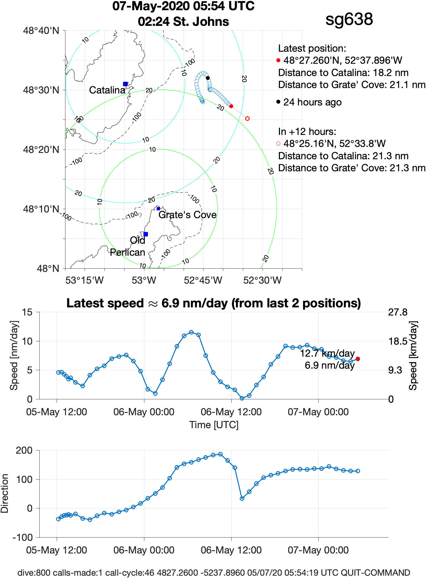
Figure 10 Emergency recovery by Memorial of a Seaglider (sg638) in Newfoundland and Labrador. Top panel shows the glider drift track after the primary batteries died and before recovery from a fishing boat. Also shown are the ultimate recovery harbor of Old Perlican and concentric rings with distance 10 and 20 NM. Bottom panels show the drift direction and speed of the glider at surface (figure courtesy of Eleanor Frajka-Williams).

In summary, when encountering emergencies in a glider deployment or difficulties managing the glider:

• Know the weather near the glider as well as the forecast for the next few days.

• Minimize time at the surface. If currents are strong, set an appropriate course to avoid head-on currents and attempt to fly under the currents if dealing with surface currents. If trapped in an eddy steer 90 degrees to get out of the eddy.

• To conserve battery power, reduce diving angles to slow the vehicle and reduce the number of inflections (e.g., 20° for Slocum, 15° for SeaExplorer), use low power mode if available, turn off the altimeter if not needed and dive deeper depth. If possible, reduce or turn off science sensor sampling.

• Limit satellite transmission times. If real-time data is not essential, consider downloading less data. However, consideration should be made regarding sending some subsampled live data in case the glider is lost and the entire dataset becomes unavailable.

• Develop a daily checklist of glider flight diagnostics to check. Examples include roll, pitch, vacuum, science data acquisition, desired heading/velocity, leak detects, symmetry of yo, battery consumption and voltage, appropriate surfacing intervals, errors and warning.

5 Glider sensor and data management

The last section focused on the knowledge and practices, operating gliders in Atlantic Canada. The goal of glider missions lies in collecting data of sufficient quality to meet the particular objectives of a particular mission. We discussed some aspects in which data quality can be constrained by operational choices (duty cycling, power constraints). Here we discuss sensor payloads employed in glider missions and practices around managing their data during and post deployment.

5.1 Glider sensor payloads

The focus of glider deployments are the sensor payload. Not all sensors developed for ship-based or mooring measurements fit a glider due to power and size-weight restrictions. Instead, gliders almost exclusively use custom sensors which are versions of sensors used on moorings and ship measurements but adapted to satisfy the limits placed on glider observations (power, dimensions, weight, sensor response time and measurement stability). CTD, O₂ optode, optical backscatter and fluorometers are standard payloads on gliders (see Figures 11A–C respectively for examples of these sensors on Slocum gliders). Examples of these recurring data streams were given in the previous section as part of the regional summary for glider activities in Atlantic Canada (see Table 1). When profiling through cold water lens (T<0°C), careful post-processing quality control is often needed to avoid spurious results caused by sharp temperature changes. Another critical aspect common to all glider payloads is tracking metadata. For this purpose, CEOTR has developed the sensor tracker” (see Figure 12), a server-based application that glider groups in Atlantic Canada can utilize to store critical information about the glider sensors (a public repository is maintained here: https://gitlab.oceantrack.org/ceotr-public/sensor_tracker). This information could include calibration coefficients, last calibration date and other pertinent information to a glider deployment that helps glider data users understand the mission. Here we discuss various sensors used in Atlantic Canada and details related to their setup to inform the glider user community about our experience and challenges.

FIGURE 11

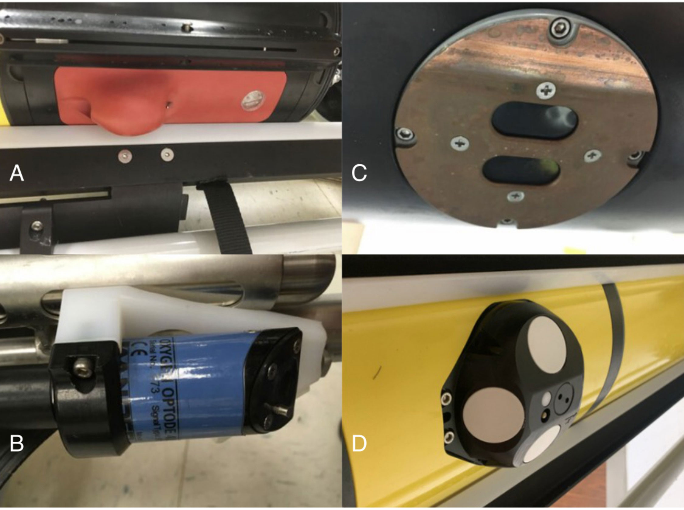
Figure 11 Selection of sensor options for gliders (A) CTD (RBR legato3 version is shown) (B) Oxygen Optode model Aanderaa 4831 with standard sensor foil; (C) Wetlabs–ECO PUCK (Chlorophyll, Backscatter and CDOM version); and (D) Specialized sensor: AD2CP glider version from NORTEK to measure magnitude and direction of ocean currents.

FIGURE 12

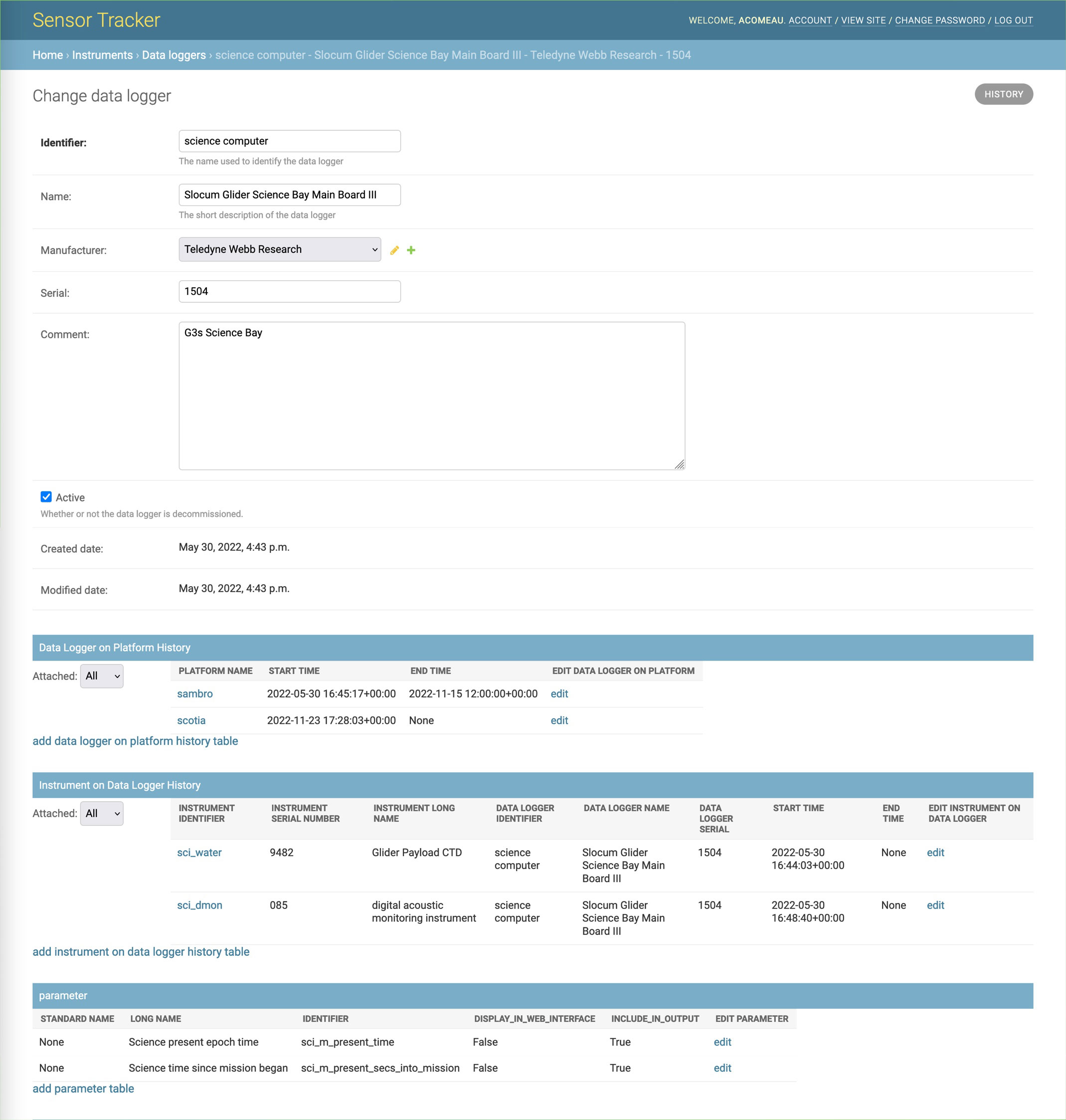
Figure 12 CEOTR Sensor tracker application (https://gitlab.oceantrack.org/ceotr-public/sensor_tracker_client) to track glider and payload metadata. Shown is a deployment of glider Scotia 711 part of the passive acoustic monitoring efforts in the Roseway Basin. The application allows exporting of metadata in JSON format and integration with glider data streams for improved data handling.

In Atlantic Canada, several different CTDs are in use, such as pumped (model SBE41 CP “GPCTD”) and unpumped (SBE 41 CTD) Seabird CTD and recently RBR legato3 CTD (inductive conductivity sensors). CTDs on gliders can make robust and reliable measurements, and sophisticated procedures exist for the Quality Control (QC) of glider CTD data (Garau et al., 2011). O₂ sensors are Aanderaa optodes (models 3830 & 4831) with either slow or fast (model 4831F) foils (Tengberg et al., 2006; Uchida et al., 2008). DFO has several RINKO and Seabird SBE43F membrane O₂ sensors (Martini et al., 2007). Various optical sensors can be used, predominantly the Wetlabs (Seabird) Eco Pucks with three measurement channels (fluorescence or backscatter). Channels are typically backscatter, chlorophyll and CDOM. DFO has been utilizing the miniFLUO-UV sensors (Cyr et al., 2019) that can assist in the detection of dissolved hydrocarbons. Another development is the measurement of turbulence using the Microrider (Rockland Scientific) that provide micro-scale measurements of temperature and velocity shear from which the dissipation rate of turbulent kinetic energy can be derived (Lueck, 2008). This sensor has improved the glider community’s knowledge of micro-scale processes and has been deployed in various glider projects in the Gulf and Atlantic (CEOTR). In general the frequency of sensor calibrations is dependent on the nature of the projects, as some require more stringent assurance of sensor accuracy. In general manufacturer recommendations for sensor calibrations are adhered to for CTDs (every 2–3 years). Memorial has been using in-house calibrations to extend the period between manufacturer calibrations on some glider deployments. For Memorial and CEOTR oxygen optodes have been calibrated in-house through the CERC.Ocean laboratory at Dalhousie University.

In the last ten years, passive and active acoustics (single and multi-frequency sounders) have increasingly been deployed on gliders, particularly in Atlantic Canada and the US. The CEOTR team and WHOI have adopted the DMON (Davis et al., 2016) for real-time and archival analysis of baleen whale calls. The DMON (Baumgartner and Mussoline, 2011) system has been licensed to Teledyne Webb Research and is integrated into the science bay of the glider or a separate payload bay. Most DMON systems are equipped with low, mid and high-frequency hydrophones. Firmware must be loaded to the science computer to record specific intervals. Because passive acoustic data files are much larger than standard glider sensor data, this data cannot be transmitted in raw format. An onboard computer inside the DMON processes the audio recordings using Low-Frequency Detection and Classification System (LFDCS) software (Baumgartner and Mussoline, 2011) based on a pre-programmed call library. Pitch tracks, obtained from a contour following an algorithm applied to a spectrogram, statistics from the LFDCS algorithm, background spectra and system diagnostics are sent to the glider, which can then be sent to shore. This provides the location of possible detection events that can be validated by shore-based analysts (Baumgartner et al., 2013). The JASCO Observer (Moloney et al., 2018) is another passive acoustic monitoring system used by DFO/CEOTR/Memorial and provides similar information to the DMON system. Predominantly, a single hydrophone sensor mounted on top of the vehicle is used, but different hydrophone configurations are available. Memorial has recently begun using a glider with wing-mounted hydrophones providing separation between hydrophones.

Glider-based active acoustic sensors have been available to measure currents (see Figure 11D) for an example of a Nortek 1 Mhz glider-mounted Acoustic Doppler Velocity Profiler (ADCP) sensor). Recent interests in marine protected areas (MPA) monitoring (Gulf, Arctic, Labrador) and fisheries science (DFO, Memorial) have pushed the development of the Acoustic Zooplankton Fish Profiler (AZFP) developed by ASL Ltd (Chave et al., 2018). This sensor carries several transducers and can be used to detect fish count and biomass. Active acoustics do not allow real-time access to raw data like passive acoustics. The AZFP and ADCP data analysis is carried out at the end of the mission. However, their use in Atlantic Canada has been limited due to the challenge associated with power consumption and sensor size. Sonars have been integrated (Memorial) for detecting the ice edge for iceberg mapping and under-ice navigation. Experiments (Zhou et al., 2019) have demonstrated their utility, particularly in future applications related to ice-shelf monitoring.

Specialized biogeochemical sensors are another recent focus of glider sensor development. Measurements of CO₂, pH and nitrate concentrations are lacking. Reliable measurements are not yet made in Atlantic Canada, but glider groups are working on implementing new sensors. Memorial and CEOTR have been conducting experimental testing with prototype pCO₂ (Atamanchuk et al., 2014; von Oppeln-Bronikowski et al., 2021a) and ISFET pH sensors (Branham et al., 2016; Johnson et al., 2016) on gliders. CEOTR is the only group to have implemented the SUNA UV (Carrol et al., 2007) Nitrate sensor (Comeau et al., 2007). This sensor has shown promising results elsewhere (e.g., Karstensen et al. (2017)), but challenges around power consumption and maintenance have precluded routine observations in Atlantic Canadian glider programs. Progress on new development of BGC sensors has been slow. The typical workload to support glider-based observations of CO₂ variables is much higher than standard measurements (CTD, O₂, Chl-a) due to the need to reference and verify the data with bottle samples carefully.

5.2 Glider data streams

Glider sensor data have specific challenges inherent to the platform. There are two approaches, to data processing: near-real-time (during deployment) and delayed mode data (after glider recovery). Processing glider data is a challenging task requiring specific expertise with the vehicles and sensors and remains a time-consuming process to achieve high-quality data. However, such intense data processing is only sometimes necessary. In general, it is now easier to transmit more data back to the users allowing for more accurate Quality Control (QC) even in real-time. Most T, S and O₂ data received in real-time from gliders are precise enough to be used to detect anomalies in ocean structure and feed global ocean assimilation models. The data are regularly sent to the Global Telecommunication System (GTS) stream (see Vargas et al. (2019) on the impact of real-time glider data on hurricane forecasting). In Atlantic Canada, data is sent to the Canadian Integrated Ocean Observing System (CIOOS) (Whoriskey et al., 2017) to facilitate broad access (Memorial/CEOTR). DFO data resides in the Marine Environmental Data Section (MEDS) Ocean Database (Anh Tran, personal communication). Memorial and CEOTR provide a web access point for real-time and delayed mode quality-controlled data (https://www.mungliders.com and https://ceotr.ocean.dal.ca/, respectively), broadening access and use of the data.

5.2.1 Realtime quality control

At a minimum, one should have some checks in glider data to flag data that is outside an expected range of the data by two standard deviations or has a constant value. Most often, a quick visual inspection reveals these inconsistencies or sensor errors. Sophisticated correction relating to the physical operation of the sensors is usually possible, for example, thermal lag correction (Bishop, 2008; Garau et al., 2011). However, others, such as the correction of the boundary layer flow around the oxygen optode foil (Bittig et al., 2014; Bittig et al., 2018), require both up and downcast data, so it may not always be possible to implement in real-time data streams. Determining vertical velocities from the glider movement is also not usually possible in real-time unless all the data are relayed. The choice of how glider data is subsampled dictates the file size necessary for Iridium transmission but also can limit the usefulness of the data. Some gliders like Slocum need more explicit settings by the user for downloading data compared to SeaExplorer. The environmental conditions in the North Atlantic further limit this since Iridium communications could be interrupted by large waves forcing the glider antenna beneath the ocean surface, cutting the connection. Communicating with a glider over a satellite in the field can take tens of seconds to minutes. This is typically more difficult at higher latitudes because of satellite limitations.

5.2.2 Delayed mode quality control

Treatment of this topic has been covered extensively by several other groups and best practices sections. We note Ocean Glider’s best practices with SOPs for salinity, O₂ and other variables (https://github.com/OceanGlidersCommunity) and the recent comprehensive IOOS guides (https://ioos.noaa.gov/project/qartod/). All Atlantic Canadian glider groups implement standard corrections. Glider CTD data is corrected for thermal lag correction (Garau et al., 2011). For oxygen optodes, there are response time and boundary layer/flow corrections (Bittig et al., 2014; Bittig et al., 2018). Figure 13 shows an example of O₂ glider data applying delayed mode QC following the OceanGliders community best practices. The glider oxygen optode calibrated phase data exhibited a 10-40 s delay between up/down casts due to sensor response coupled with uneven dive/climb dive speeds and flow across the sensor surface. A moving median delay is used (Woo and Gourcuff, 2021). Optical channels such as backscatter and chlorophyll tend to be not calibrated in the lab, except for offsets (see Thomalla et al. (2018) for a thorough discussion on QC for optical backscattering sensors). For the best data quality, consideration should be given to independently verifying glider data before, during, and at the end of deployments. Usually, during deployment/recovery, it is possible to conduct independent ship-based CTD casts with a well-calibrated CTD system. In-situ checks for glider data are also possible such as the in-air correction for optodes (example in Nicholson and Feen (2017)). We recommended comparing CTD and other sensors with nearby measurements from Argo or ships when available to ascertain data validity.

FIGURE 13

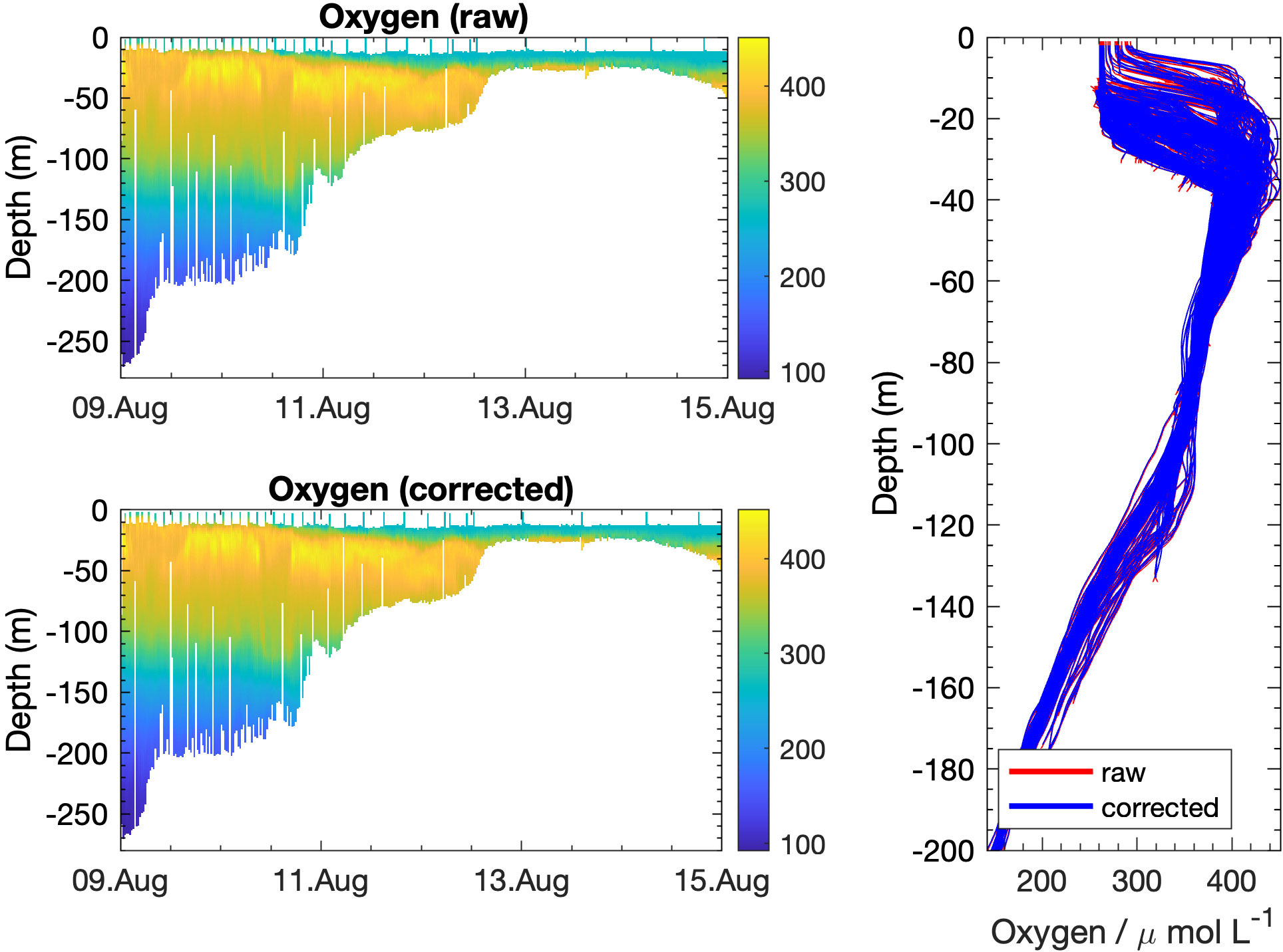
Figure 13 Example oxygen data corrections for Slocum glider data collected with an Aanderaa 4831 optode equipped with a standard (black) foil. The upper panel is the raw oxygen data from the glider and the lower panel is the correction applied from (Bittig et al., 2014, 2018). The color bar shows oxygen concentration in units of micro-moles L^-1. The response time correction appears to work well, except in the upper thermocline where the strong temperature gradient (1°C m^-1) and unequal dive/climb rates caused a shift of the oxygen data due to the sensor’s slow response.

6 Summary and future outlook

This paper summarized the history and status of glider activities in Atlantic Canada and the experience gained from operating in this environment. The following critical elements of glider operations were covered:

1. Regional oceanographic and geographic context

2. Operational considerations

3. Lessons learned on framing glider activities in Atlantic Canada in a sustainable program context.

There are several different groups operating gliders in Atlantic Canada with programs related to acoustic monitoring and tracking, process studies and environmental monitoring. The programs and projects that sustain these operations are designed around the observing needs of academic research, government monitoring programs and some linkages to Non Governmental Organizations (NGO’s) and the private sector. The dominant focus of sustained glider deployments is on the Scotian Shelf and in the Gulf of St. Lawrence, mirroring regional ocean observing needs of the Canadian Government (e.g., AZMP). Most of these glider deployments are focused on the shallow continental shelf. A prominent and continuously increasing focus of these missions is on passive acoustics supporting Transport Canada to reduce the impact of marine traffic on whales. Other projects, such as winter deployments in the Labrador Sea, demonstrate the reliability of the equipment in harsh ocean conditions. The ability of gliders to operate in polar and open ocean environments makes them an attractive option that is much less expensive than a ship-based program. These applications of gliders illustrate the benefits of these vehicles in Atlantic Canada.

We provided insights on the many benefits, costs and capabilities of glider programs and how these could be organized in the context of the Atlantic Canadian experience. Gliders have a steady global footprint in ocean observation (Testor et al., 2019), including in Atlantic Canada. However, only a few of the many applications that gliders can be used for have been so far carried out as a sustained effort. Moreover, even though gliders are cheaper than ships to operate. We discuss this discrepancy noting that the value of glider data has not been fully realized. For example, the pragmatic focus on passive acoustics with gliders has demonstrated clear value by providing the necessary data over a targeted area at a low cost (Baumgartner et al., 2013; Davis et al., 2016). This has resulted in stable glider programs in this application. However, the value from gliders has not been fully utilized for applications like ocean region monitoring or climate change.

The summary of operational best practices should be a valuable guide to those interested in glider data or glider deployments, and the experience of using gliders in Atlantic Canada has taught many lessons. Critical aspects of glider operations vary depending on the mission profile. The limited endurance of gliders highlights the need for the careful prior setup of the vehicle. Suggestions for power management in all glider mission stages, based on best practices and operational experience, have been summarized. Some of the main concerns arising from glider operations in Atlantic Canada are tied to recovery and emergency plans, given the limited availability of ships and the often-poor weather conditions. Strong currents, severe weather and strong tides make planning essential. We present approaches for mission planning, such as the recent OceanGNS (von Oppeln-Bronikowski et al., 2021b) that originated from operational glider experience in the Labrador Sea.

The use of gliders as part of Atlantic Canada’s ocean observation is likely to grow. The technology has matured, and its use as a central sampling platform continues to expand (see Testor et al. (2019)). The glider community continues to develop further best practices on glider operational protocols, in particular data treatment and forums for knowledge exchange (see for example Ocean Glider Community pages, US IOOS UG2 group). Our paper summarizes the experience from operating gliders in Atlantic Canada over the past 18 years, and sharing this experience is valuable on a global context. In Atlantic Canada, we believe that using gliders in harsh environments like the Labrador Sea in providing a vital link between regional and global climate observations demonstrates the reach of regional glider capabilities. While the need for glider systems is clear, we must work as a community to share our experiences to ensure that we gain the most from these competent sampling tools.

Ethics statement

Written informed consent was obtained from the individual(s) for the publication of any identifiable images or data included in this article.

Author contributions

NvOB and BdY conceived and wrote the initial draft paper. RD, BdY, DH, and PE obtained funding to establish the respective glider groups. FC, AC, JM, and MB provided figures and significant editorial contributions. All authors contributed towards editing and revisions of the paper. All authors contributed to the article and approved the submitted version.

Funding

Memorial gliders are funded through the Ocean Frontier Institute under Module O “Transforming Ocean Observations”, the Marine Environmental Observation, Prediction and Response Network (MEOPAR), the Natural Sciences and Engineering Research Council (NSERC) and the Canada Foundation for Innovation (CFI) founded Development of Autonomous Marine Observation Systems (DAMOS) Program. CEOTR acknowledges funding from the Ocean Tracking Network (OTN), OFI, MEOPAR and CFI (DAMOS).

Acknowledgments

We acknowledge the thoughtful feedback and comments from two reviewers who greatly improved the manuscript. DFO glider work partly contributes to the scientific mission of the Atlantic Zone Monitoring Program. FC would like to thank R. Stagg and DFO's Conservation and Protection fisheries officer for making the glider deployments in Bonavista possible.

Conflict of interest

The authors declare that the research was conducted in the absence of any commercial or financial relationships that could be construed as a potential conflict of interest.

Publisher’s note

All claims expressed in this article are solely those of the authors and do not necessarily represent those of their affiliated organizations, or those of the publisher, the editors and the reviewers. Any product that may be evaluated in this article, or claim that may be made by its manufacturer, is not guaranteed or endorsed by the publisher.

References

Atamanchuk D., Tengberg A., Thomas P. J., Hovdenes J., Apostolidis A., Huber C., et al. (2014). Performance of a lifetime-based optode for measuring partial pressure of carbon dioxide in natural waters. Limnology Oceanogr.: Methods 12, 63–73. doi: 10.4319/lom.2014.12.63

CrossRef Full Text | Google Scholar

Banks R. (1966). The cold layer in the Gulf of St. Lawrence. J. Geophysical Res. 71, 1603–1610. doi: 10.1029/JZ071i006p01603

CrossRef Full Text | Google Scholar

Baumgartner M. F., Fratantoni D. M., Hurst T. P., Brown M. W., Cole T. V., Van Parijs S. M., et al. (2013). Real-time reporting of baleen whale passive acoustic detections from ocean gliders. J. Acoustical Soc. America 134, 1814–1823. doi: 10.1121/1.4816406

CrossRef Full Text | Google Scholar

Baumgartner M. F., Mussoline S. E. (2011). A generalized baleen whale call detection and classification system. J. Acoustical Soc. America 129, 2889–2902. doi: 10.1121/1.3562166

CrossRef Full Text | Google Scholar

Baumgartner M. F., Stafford K. M., Latha G. (2018). Near real-time underwater passive acoustic monitoring of natural and anthropogenic sounds. Observing Oceans Real Time, 203–226. doi: 10.1007/978-3-319-66493-4_10

CrossRef Full Text | Google Scholar

Bishop C. M. (2008). Sensor dynamics of of autonomous underwater gliders. Master’s (Memorial University of Newfoundland).

Google Scholar

Bittig H. C., Fiedler B., Scholz R., Krahmann G., Körtzinger A. (2014). Time response of oxygen optodes on profiling platforms and its dependence on flow speed and temperature. Limnology Oceanogr.: Methods 12, 617–636. doi: 10.4319/lom.2014.12.617

CrossRef Full Text | Google Scholar

Bittig H. C., Körtzinger A. (2015). Tackling oxygen optode drift: near-surface and in-air oxygen optode measurements on a float provide an accurate in situ reference. J. Atmospheric Oceanic Technol. 32, 1536–1543. doi: 10.1175/JTECH-D-14-00162.1

CrossRef Full Text | Google Scholar

Bittig H. C., Körtzinger A., Neill C., Van Ooijen E., Plant J. N., Hahn J., et al. (2018). Oxygen optode sensors: principle, characterization, calibration, and application in the ocean. Front. Mar. Sci. 4, 429. doi: 10.3389/fmars.2017.00429

CrossRef Full Text | Google Scholar

Branham C. W., Murphy D., Johnson K., Jannasch H. (2016). Optimization of a robust and reliable ISFET sensor for measuring pH in the deep ocean, in OCEANS 2016 MTS/IEEE Monterey (IEEE), 1–4. doi: 10.1109/OCEANS.2016.7761357

CrossRef Full Text | Google Scholar

Broecker W. S., Virgilio A., Peng T.-H. (1991). Radiocarbon age of waters in the deep Atlantic revisited. Geophysical Res. Lett. 18, 1–3. doi: 10.1029/90GL02707

CrossRef Full Text | Google Scholar

Carrol M., Chigounis D., Cook J., Gilbert S., Johengen T., Koles T., et al. (2007). Performance demonstration statement satlantic ISUS V3 nitrate sensor (Tech. rep., Satlantic Inc). doi: 110.25607/OBP-350

Google Scholar

Chassignet E. P., Hurlburt H. E., Smedstad O. M., Halliwell G. R., Hogan P. J., Wallcraft A. J., et al. (2007). The HYCOM (hybrid coordinate ocean model) data assimilative system. J. Mar. Syst. 65, 60–83. doi: 10.1016/j.jmarsys.2005.09.016

CrossRef Full Text | Google Scholar

Chave R., Buermans J., Lemon D., Taylor J. C., Lembke C., DeCollibus C., et al. (2018). Adapting multi-frequency echo-sounders for operation on autonomous vehicles, in OCEANS 2018 MTS/IEEE Charleston (IEEE). 1–6. doi: 10.1016/j.jmarsys.2005.09.016

CrossRef Full Text | Google Scholar

Claus B., Bachmayer R. (2015). Terrain-aided navigation for an underwater glider. J. Field Robotics 32, 935–951. doi: 10.1002/rob.21563

CrossRef Full Text | Google Scholar

Claus B., Bachmayer R., Williams C. D. (2010). Development of an auxiliary propulsion module for an autonomous underwater glider. Proc. Institution Mechanical Engineers Part M: J. Eng. Maritime Environ. 224, 255–266. doi: 10.1243/14750902JEME204

CrossRef Full Text | Google Scholar

Colbourne E. (2004). The history of standard hydrographic sections in Newfoundland and Labrador. AZMP Bull. (Ottawa, Ontario: Fisheries and Oceans Canada), Bulletin PMZA Atlantic Zone Monitoring Program Bulletin, 4, 29–33.

Google Scholar

Comeau A., Lewis M., Cullen J., Adams R., Andrea J., Feener S., et al. (2007). Monitoring the spring bloom in an ice covered fjord with the Land/Ocean biogeochemical observatory (LOBO), in OCEANS 2007 (IEEE). 1–7. doi: 10.1109/OCEANS.2007.4449185

CrossRef Full Text | Google Scholar

Crickard F. (1995). Canada’s ocean and maritime security a strategic forecast: a strategic forecast. Mar. Policy 19, 335–342. doi: 10.1016/0308-597X(95)00012-U

CrossRef Full Text | Google Scholar

Cyr F., Bourgault D., Galbraith P. (2011). Interior versus boundary mixing of a cold intermediate layer. J. Geophysical Research: Oceans 116. doi: 10.1029/2011JC007359

CrossRef Full Text | Google Scholar

Cyr F., Galbraith P. S. (2021). A climate index for the Newfoundland and Labrador shelf. Earth System Sci. Data 13, 1807–1828. doi: 10.5194/essd-13-1807-2021

CrossRef Full Text | Google Scholar

Cyr F., Tedetti M., Besson F., Bhairy N., Goutx M. (2019). A glider-compatible optical sensor for the detection of polycyclic aromatic hydrocarbons in the marine environment. Front. Mar. Sci. 6, 110. doi: 10.3389/fmars.2019.00110

CrossRef Full Text | Google Scholar

Davis R., Baumgartner M., Comeau A., Cunningham D., Davies K., Furlong A., et al. (2016). Tracking whales on the scotian shelf using passive acoustic monitoring on ocean gliders, in OCEANS 2016 MTS/IEEE Monterey (IEEE). 1–4. doi: 10.1109/OCEANS.2016.7761461

CrossRef Full Text | Google Scholar

Davis R., Comeau A., L’Orsa S., van der Meer J., Covey B., Pye J., et al. (2018). Lessons learned in developing a Canadian operational glider fleet. Mar. Technol. Soc. J. 52, 13–18. doi: 10.4031/MTSJ.52.3.20

CrossRef Full Text | Google Scholar

Davis R. E., Eriksen C. C., Jones C. P. (2002). Autonomous buoyancy-driven underwater gliders. Technol. Appl. autonomous underwater vehicles 3, 37–58. doi: 10.1201/9780203522301.ch3

CrossRef Full Text | Google Scholar

de Fommervault O., Besson F., Beguery L., Le Page Y., Lattes P. (2019). SeaExplorer underwater glider: a new tool to measure depth-resolved water currents profiles, in OCEANS 2019-Marseille (IEEE). 1–6. doi: 10.1109/OCEANSE.2019.8867228

CrossRef Full Text | Google Scholar

Dever M., Hebert D., Greenan B., Sheng J., Smith P. (2016). Hydrography and coastal circulation along the Halifax line and the connections with the Gulf of St. Lawrence. Atmosphere-Ocean 54, 199–217. doi: 10.1080/07055900.2016.1189397

CrossRef Full Text | Google Scholar

de Young B., Frajka-Williams E., von Oppeln-Bronikowski N., Woodward S. (2020). Technicalities: exploring the Labrador Sea with autonomous vehicles. J. Ocean Technol. 15, 134–139.

Google Scholar

de Young B., Peterman R., Dobell A., Pinkerton E., Breton Y., Charles A., et al. (1999). Canadian Marine fisheries in a changing and uncertain world: a report prepared for the Canadian global change program of the royal society of Canada. Fisheries Aquat. Sci. 129, 199.

Google Scholar

de Young B., Rose G. A. (1993). On recruitment and distribution of Atlantic cod. Can. J. Fisheries Aquat. Sci. 50, 2729–2741. doi: 10.1139/f93-298

CrossRef Full Text | Google Scholar

Eriksen C. C., Rhines P. (2008). Convective to gyre-scale dynamics: seaglider campaigns in the Labrador Sea 2003–2005, in Arctic–Subarctic ocean fluxes (Springer), 613–628. doi: 10.1007/978-1-4020-6774-726

CrossRef Full Text | Google Scholar

Fisheries and Oceans Canada (2021). Canada’s fisheries fast facts 2021, in Economic analysis and statistics report, DFO. Available at: https://waves-vagues.dfompo.gc.ca/Library/41039634.pdf?

Google Scholar

Florindo-López C., Bacon S., Aksenov Y., Chafik L., Colbourne E., Holliday N. P. (2020). Arctic Ocean and Hudson bay freshwater exports: new estimates from seven decades of hydrographic surveys on the Labrador shelf. J. Climate 33, 8849–8868. doi: 10.1175/JCLI-D-19-0083.1

CrossRef Full Text | Google Scholar

Frajka-Williams E., Rhines P. B., Eriksen C. C. (2009). Physical controls and mesoscale variability in the Labrador Sea spring phytoplankton bloom observed by seaglider, in Deep Sea Research Part I: Oceanographic Research Papers, vol. 56, 2144–2161. doi: 10.1016/j.dsr.2009.07.008

CrossRef Full Text | Google Scholar

Frajka-Williams E., Rhines P. B., Eriksen C. C. (2014). Horizontal stratification during deep convection in the Labrador Sea. J. Phys. oceanogr. 44, 220–228. doi: 10.1175/JPO-D-13-069.1

CrossRef Full Text | Google Scholar

Garau B., Ruiz S., Zhang W. G., Pascual A., Heslop E., Kerfoot J., et al. (2011). Thermal lag correction on Slocum CTD glider data. J. Atmospheric Oceanic Technol. 28, 1065–1071. doi: 10.1175/JTECH-D-10-05030.1

CrossRef Full Text | Google Scholar

GEBCO (2022). GEBCO 2022 grid. doi: 10.5285/e0f0bb80-ab44-2739-e053-6c86abc0289c

CrossRef Full Text | Google Scholar

Gilbert D., Sundby B., Gobeil C., Mucci A., Tremblay G.-H. (2005). A seventy-two-year record of diminishing deep-water oxygen in the St. Lawrence estuary: the northwest Atlantic connection. Limnology Oceanogr. 50, 1654–1666. doi: 10.4319/lo.2005.50.5.1654

CrossRef Full Text | Google Scholar

Hátún H., Eriksen C. C., Rhines P. B. (2007). Buoyant eddies entering the Labrador Sea observed with gliders and altimetry. J. Phys. Oceanogr. 37, 2838–2854. doi: 10.1175/2007JPO3567.1

CrossRef Full Text | Google Scholar

Howatt T., Palter J. B., Matthews J. B. R., de Young B., Bachmayer R., Claus B. (2018). Ekman and eddy exchange of freshwater and oxygen across the Labrador shelf break. J. Phys. Oceanogr. 48, 1015–1031. doi: 10.1175/JPO-D-17-0148.1

CrossRef Full Text | Google Scholar

Hughes J. (2019). Assessment of needs and opportunities for research vessel use in Atlantic Canada (Halifax, Canada: Tech. rep., Marine Environmental Observation, Prediction and Response Network (MEOPAR).

Google Scholar

Johnson K. S., Jannasch H. W., Coletti L. J., Elrod V. A., Martz T. R., Takeshita Y., et al. (2016). Deep-Sea DuraFET: a pressure tolerant pH sensor designed for global sensor networks. Analytical Chem. 88, 3249–3256. doi: 10.1021/acs.analchem.5b04653

CrossRef Full Text | Google Scholar

Jones C., Allsup B., DeCollibus C. (2014). Slocum Glider: expanding our understanding of the oceans, in 2014 Oceans-St. John’s (IEEE). 1–10. doi: 10.1109/OCEANS.2014.7003260

CrossRef Full Text | Google Scholar

Jutras M., Dufour C., Mucci A., Cyr F., Gilbert D. (2020). Temporal changes in the causes of the observed oxygen decline in the st. Lawrence estuary. J. Geophysical Research: Oceans 125, e2020JC016577. doi: 10.1029/2020JC016577

CrossRef Full Text | Google Scholar

Karstensen J., Schütte F., Pietri A., Krahmann G., Fiedler B., Grundle D., et al. (2017). Upwelling and isolation in oxygen-depleted anticyclonic modewater eddies and implications for nitrate cycling. Biogeosciences 14, 2167–2181. doi: 10.5194/bg-14-2167-2017

CrossRef Full Text | Google Scholar

Lab Sea Group (1998). The Labrador Sea deep convection experiment, in Bulletin of the American Meteorological Society, Vol. 79. 2033–2058. doi: 10.1175/1520-0477(1998)079-2033:TLSDCE?2.0.CO;2

CrossRef Full Text | Google Scholar

Landschützer P., Gruber N., Bakker D. C., Schuster U. (2014). Recent variability of the global ocean carbon sink. Global Biogeochem. Cycles 28, 927–949. doi: 10.1002/2014GB004853

CrossRef Full Text | Google Scholar

Liblik T., Karstensen J., Testor P., Alenius P., Hayes D., Ruiz S., et al. (2016). Potential for an underwater glider component as part of the global ocean observing system. Methods Oceanogr. 17, 50–82. doi: 10.1016/j.mio.2016.05.001

CrossRef Full Text | Google Scholar

Lotze H. K., Milewski I. (2004). Two centuries of multiple human impacts and successive changes in a North Atlantic food web. Ecol. Appl. 14, 1428–1447. doi: 10.1890/03-5027

CrossRef Full Text | Google Scholar

Lozier M. S., Li F., Bacon S., Bahr F., Bower A. S., Cunningham S., et al. (2019). A sea change in our view of overturning in the subpolar North Atlantic. Science 363, 516–521. doi: 10.1126/science.aau6592

PubMed Abstract | CrossRef Full Text | Google Scholar

Lueck R. (2008). Testing of the EAWAG VMP-500 SN: 028 in Harry lake, (Tech. rep., Rockland Scientific Ltd).

Google Scholar

Macdonald R. S. J. (1966). The Arctic frontier (University of Toronto Press).

Google Scholar

Martini M., Butman B., Mickelson M. J. (2007). Long-term performance of aanderaa optodes and Sea-bird SBE-43 dissolved-oxygen sensors bottom mounted at 32 m in Massachusetts bay. J. Atmospheric Oceanic Technol. 24, 1924–1935. doi: 10.1175/JTECH2078.1

CrossRef Full Text | Google Scholar

McDougall T. J., Barker P. M. (2011). Getting started with TEOS-10 and the Gibbs seawater (GSW) oceanographic toolbox. Scor/Iapso WG 127, 1–28.

Google Scholar

Merckelbach L. (2013). On the probability of underwater glider loss due to collision with a ship. J. Mar. Sci. Technol. 18, 75–86. doi: 10.1007/s00773-012-0189-7

CrossRef Full Text | Google Scholar

Moloney J., Cole A., Hillis C., Kowarski K., MacDonald B., Pedersen G., et al. (2018). Observer AMAR G4 passive acoustic monitoring system for autonomous maritime observation, in 2018 IEEE/OES Autonomous Underwater Vehicle Workshop (AUV) (IEEE). 1–9. doi: 10.1109/AUV.2018.8729796

CrossRef Full Text | Google Scholar

Nicholson D. P., Feen M. L. (2017). Air calibration of an oxygen optode on an underwater glider. Limnology Oceanogr.: Methods 15, 495–502. doi: 10.1002/lom3.10177

CrossRef Full Text | Google Scholar

Ordoñez C. E., Barth J. A., Roughan M. (2021). Boundary ocean observation network for the global south. Mar. Technol. Soc. J. 55, 80–81. doi: 10.4031/MTSJ.55.3.30

CrossRef Full Text | Google Scholar

Petrie B. (1988). The cold intermediate layer on the Labrador and northeast Newfoundland shelves 1978-1986. NAFO Sci. Counc. Stud. 12, 57–69. doi: 10.1080/07055900.1988.9649301

CrossRef Full Text | Google Scholar

Petrie B., Toulany B., Garrett C. (1988). The transport of water, heat and salt through the Strait of Belle Isle. Atmosphere-Ocean 26, 234–251. doi: 10.1080/07055900.1988.9649301

CrossRef Full Text | Google Scholar

Ricketts P., Harrison P. (2007). Coastal and ocean management in Canada: moving into the 21st century. Coast. Manage 35, 5–22. doi: 10.1080/10.1080/08920750600970545

CrossRef Full Text | Google Scholar

Roemmich D., Johnson G. C., Riser S., Davis R., Gilson J., Owens W. B., et al. (2009). The Argo program: observing the global ocean with profiling floats. Oceanography 22, 34–43. doi: 10.5670/oceanog.2009.36

CrossRef Full Text | Google Scholar

Rudnick D. L., Davis R. E., Eriksen C. C., Fratantoni D. M., Perry M. J. (2004). Underwater gliders for ocean research. Mar. Technol. Soc. J. 38, 73–84. doi: 10.4031/002533204787522703

CrossRef Full Text | Google Scholar

Sabine C. L., Feely R. A., Gruber N., Key R. M., Lee K., Bullister J. L., et al. (2004). The oceanic sink for anthropogenic CO₂. Science 305, 367–371. doi: 10.1126/science.1097403

PubMed Abstract | CrossRef Full Text | Google Scholar

Simard Y., Lepage R., Gervaise C. (2010). Anthropogenic sound exposure of marine mammals from Seaways: estimates for lower St. Lawrence Seaway, eastern Canada. Appl. Acoustics 71, 1093–1098. doi: 10.1016/j.apacoust.2010.05.012

CrossRef Full Text | Google Scholar

Smith P. C., Petrie B. D. (1982). Low-frequency circulation at the edge of the scotian shelf. J. Phys. Oceanogr. 12, 28–46. doi: 10.1175/1520-0485(1982)012<0028:LFCATE>2.0.CO;2

CrossRef Full Text | Google Scholar

Smith G. C., Roy F., Brasnett B. (2013). Evaluation of an operational ice–ocean analysis and forecasting system for the Gulf of St. Lawrence. Q. J. R. Meteorol. Soc. 139, 419–433. doi: 10.1002/qj.1982

CrossRef Full Text | Google Scholar

Talley L. D., McCartney M. S. (1982). Distribution and circulation of Labrador Sea water. J. Phys. Oceanogr. 12, 1189–1205. doi: 10.1175/1520-0485(1982)012<1189:DACOLS>2.0.CO;2

CrossRef Full Text | Google Scholar

Tengberg A., Hovdenes J., Andersson H. J., Brocandel O., Diaz R., Hebert D., et al. (2006). Evaluation of a lifetime-based optode to measure oxygen in aquatic systems. Limnology Oceanogr.: Methods 4, 7–17. doi: 10.4319/lom.2006.4.7

CrossRef Full Text | Google Scholar

Testor P., de Young B., Rudnick D. L., Glenn S., Hayes D., Lee C. M., et al. (2019). Oceangliders: a component of the integrated goos. Front. Mar. Sci. 6. doi: 10.3389/fmars.2019.00422

CrossRef Full Text | Google Scholar

Therriault J., Petrie B., Pepin P., Gagnon J., Gregory D., Helbig J., et al. (1998). Proposal for a Northwest aonal monitoring program, (Ottawa, Canada: Canadian Technical report of hydrographic and ocean sciences, DFO).

Google Scholar

Thomalla S. J., Moutier W., Ryan-Keogh T. J., Gregor L., Schütt J. (2018). An optimized method for correcting fluorescence quenching using optical backscattering on autonomous platforms. Limnology Oceanogr.: Methods 16, 132–144. doi: 10.1002/lom3.10234

CrossRef Full Text | Google Scholar

Trowbridge J., Weller R., Kelley D., Dever E., Plueddemann A., Barth J. A., et al. (2019). The ocean observatories initiative. Front. Mar. Sci. 74. doi: 10.3389/fmars.2019.00074

CrossRef Full Text | Google Scholar

Uchida H., Kawano T., Kaneko I., Fukasawa M. (2008). In situ Calibration of optode-based oxygen sensors. J. Atmospheric Oceanic Technol. 25, 2271–2281. doi: 10.1175/2008JTECHO549.1

CrossRef Full Text | Google Scholar

Vargas M. A., Miles T., Glenn S., Hogan P., Wilson W. D., Watlington R., et al. (2019). Impact of glider data assimilation on the global ocean forecasting system during the 2018 hurricane season, in OCEANS 2019 MTS/IEEE SEATTLE (IEEE). 1–5. doi: 10.23919/OCEANS40490.2019.8962824

CrossRef Full Text | Google Scholar

von Oppeln-Bronikowski N., de Young B., Atamanchuk D., Wallace D. W. R. (2021a). Glider-based observations of CO₂ in the Labrador Sea. Ocean Sci. 17, 1–16. doi: 10.5194/os-17-1-2021

CrossRef Full Text | Google Scholar

von Oppeln-Bronikowski N., Zhou M., Bahadory T., de Young B. (2021b). Overview of a new ocean glider navigation system: OceanGNS. Front. Mar. Sci. 8, 1637. doi: 10.3389/fmars.2021.671103

CrossRef Full Text | Google Scholar

Weller R. A., Baker D. J., Glackin M. M., Roberts S. J., Schmitt R. W., Twigg E. S., et al. (2019). The challenge of sustaining ocean observations. Front. Mar. Sci. 6. doi: 10.3389/fmars.2019.00105

CrossRef Full Text | Google Scholar

Whoriskey F., Morton K., Bajona L., Beck M., Dewey R., Guillemot E., et al. (2017). Canadian Integrated Ocean Observing System Investigative Evaluations: Observations and Data. Tech. rep. CIOOS. doi: 10.15273/10222/74923

CrossRef Full Text | Google Scholar

Woo L. M., Gourcuff C. (2021). Ocean gliders delayed mode QA/QC best practice manual, in Version 3.0. tech. rep., integrated marine observing system (IMOS)(Hobart, Australia). doi: 10.26198/5c997b5fdc9bd

CrossRef Full Text | Google Scholar

Zhou M., Bachmayer R., de Young B. (2017). Underwater acoustic-based navigation towards multi-vehicle operation and adaptive oceanographic sampling, in 2017 IEEE/RSJ International Conference on Intelligent Robots and Systems (IROS) (IEEE). 6091–6097. doi: 10.1109/IROS.2017.8206508

CrossRef Full Text | Google Scholar

Zhou M., Bachmayer R., de Young B. (2019). Mapping the underside of an iceberg with a modified underwater glider. J. Field Robotics 36, 1102–1117. doi: 10.1002/rob.21873

CrossRef Full Text | Google Scholar