Flow current field observation with underwater moving acoustic tomography

1 Introduction

The development of underwater observation technology promotes the sensing and monitoring methods of marine environment (Munk & Wunsch, 1979). Coastal acoustic tomography (CAT) is an advanced technology for environment observation in the shallow waters, which is developed from ocean acoustic tomography (OAT) (Munk & Wunsch, 1979; Kaneko et al., 2020). The travel time delays obtained from the reciprocal transmission signals between sound stations are used to inverse the range-average water temperature and flow current in the observation area. In typical CAT observation experiments, inversion results are calculated using sound transmission information between sound stations in the multi-station network. This approach is of higher efficiency compared with single point measurement such as Acoustic Doppler Current Profiler (ADCP), Conductivity Temperature Depth system (CTD), Temperature Depth system (TD), etc. However, the previous method used travel time to inverse the mean variations of environment (temperature or flow) in observation area by layer-averaged or grid-averaged, without refining of all changing at each spatial position. The high precision variations at each area are necessary. In recent years, CAT technology is widely used for water parameter survey and observation in coastal water, islands region, river and so on. More advanced methods and experimental formats are proposed (Chen et al., 2021; Xiao et al., 2021; Xu et al., 2021; Chen et al., 2022; Mohamad Basel Al et al., 2022; Xu et al., 2022).

Sawaf et.al analyzed the inflow characteristics within a slow water-flow environment barrier lake via two pairs of fluvial acoustic tomography (FAT) systems, and developed an equation to estimate the flow direction (Al Sawaf et al., 2017; Al Sawaf & Kawanisi, 2018). Chen Minmo et.al conducted many studies via CAT in coastal areas for water temperature and flow current inversion (Chen et al., 2016; Chen et al., 2017; Chen et al., 2019; Chen et al., 2020; Chen et al., 2020; Chen et al., 2020; Chen et al., 2021). Recently, they found the standing-type waves by reconstructing the two-dimensional (2D) flow fields using a coast-fitting inversion model of five sound stations, which led to flood- and ebb-dominant tidal current asymmetries for the western and eastern halves in model domain, respectively (Chen et al., 2022). Besides, CAT technology was used for mapping tidal current and salinity. Kawanisi et. al continuously monitored two-dimensional distributions of current and salinity at a shallow tidal junction for 34.4 days and efficiently estimated the variations of the currents and salinity (Bahreinimotlagh et al., 2016; Kawanisi et al., 2016; Bahreinimotlagh et al., 2019; Chen et al., 2021; Xiao et al., 2021; Mohamad Basel Al et al., 2022). Future more, in order to obtain more spatially environment data, underwater moving acoustic tomography is proposed and developed. Chengfen Huang et.al achieved the first application of this method for the acoustic mapping of ocean currents in a shallow-water environment via four moored station and one ship-towed station (Huang, 2019; Huang et al., 2019). The errors of travel time difference caused by relative motion were corrected by Doppler shift estimated from the measured channel impulse response.

Unlike fix-station observations, moving sound transmission can obtain the observation of entire spatial area with sound station moving. Various internal structures, unique surface and submarine boundaries and changing environment constitutes a complex acoustic propagation channel. In particular, the problem of signal frequency drift, multi-path ray identifying need to be considered with sound station motion. This paper focus on the inversion method and signal resampling for sound moving transmission. Also, the current field in three-dimensional (3D) scale is also studied. A five-station sound transmission experiment with four moored station and one moving station that conducted at Huangcai reservoir, Changsha, China is presented. Signal resampling is performed to get correlation of received acoustic data. The vertical layer-averaged flow current results between moving station and moored station are inversed with 2D grid method (Huang et al., 2021; Xu et al., 2021; Xu et al., 2022). 3D flow current field is also reconstructed. Meanwhile, the advantage and disadvantage of underwater moving acoustic tomography are discussed.

This rest of paper is structured as follows: in Section 2, experimental settings of moving acoustic tomography is introduced. The inversion method of moving acoustic tomography and ray simulation is presented in Section 3. Section 4 focus on inversion results in 2D vertical profiles, 3D flow current field is also mapped in this section. Discussion and conclusion are given in Section 5 and Section 6, respectively.

2 Overview of experiment

An underwater moving acoustic tomography experiment was conducted with five high-frequency CAT systems at March 5th, 2022 in the Huangcai Reservoir, west of Changsha, China. Figure 1 shows the deployment of four moored stations and one moving station. Moored acoustic stations (S1-S4) were distributed at the corners of square flow confluence area, the moving acoustic station (S5) was towed with a fish boat using s 6m rope along circle and straight-line paths inside the observation area. Each moored station was fixed by a buoy and an anchored. All acoustic stations were equipped with high-frequency CAT system, 24V and 12V battery array, sound transceiver, GPS (less than 0.6μs time error) and TD (Temperature Depth Sensor). The reciprocal sound transmissions were successfully carried simultaneously between station pairs. GPS was used for time synchronisation of five stations and TD is used to record depth variations of each station.

FIGURE 1

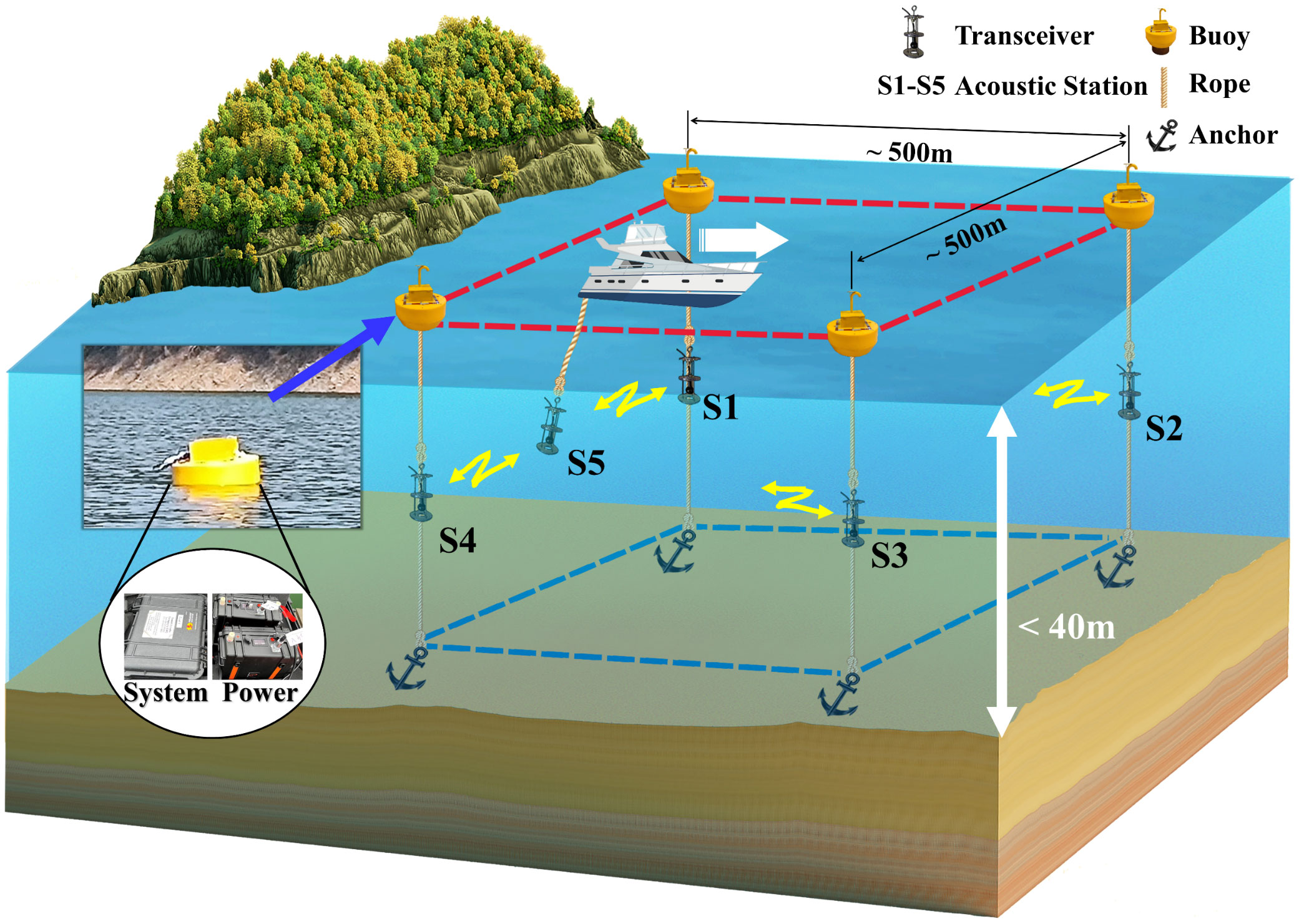
Figure 1 CAT station deployment in Huangcai Reservoir view from the north. Magnified figures with black circle show the layout of CAT system. Figure legends is shown at top right. White arrow shows the direction of motion station. The observation area is within 500m × 500m and the water depth is less than 40m.

In this experiment, sound transmissions between moving station and each moored station were analyzed. The high-frequency CAT systems that used in this experiment were developed by Hiroshima University (Kaneko et al., 2020). During the experiment, the distance between moving station and fix station is changing at range from 60m to 600m. The 9th order M-sequence phase-modulated sound signals were transmitted by transceivers; modulation depth is 2; each station was assigned a specific signal M-sequence code for code division multiple access. The signal-to-noise ratio (SNR) was improved by M-sequence of $20\log \sqrt{2^9\times 2-1}=30.098$ dB. The operation frequency range of transceiver cover 10kHz-90kHz. The center frequency of transmitted sound is 50kHz with 1-mintue transmission interval in this experiment. The length of one-period was 20.46ms (1023 bits). Table 1 shows the detail of acoustic signal and sound stations.

TABLE 1

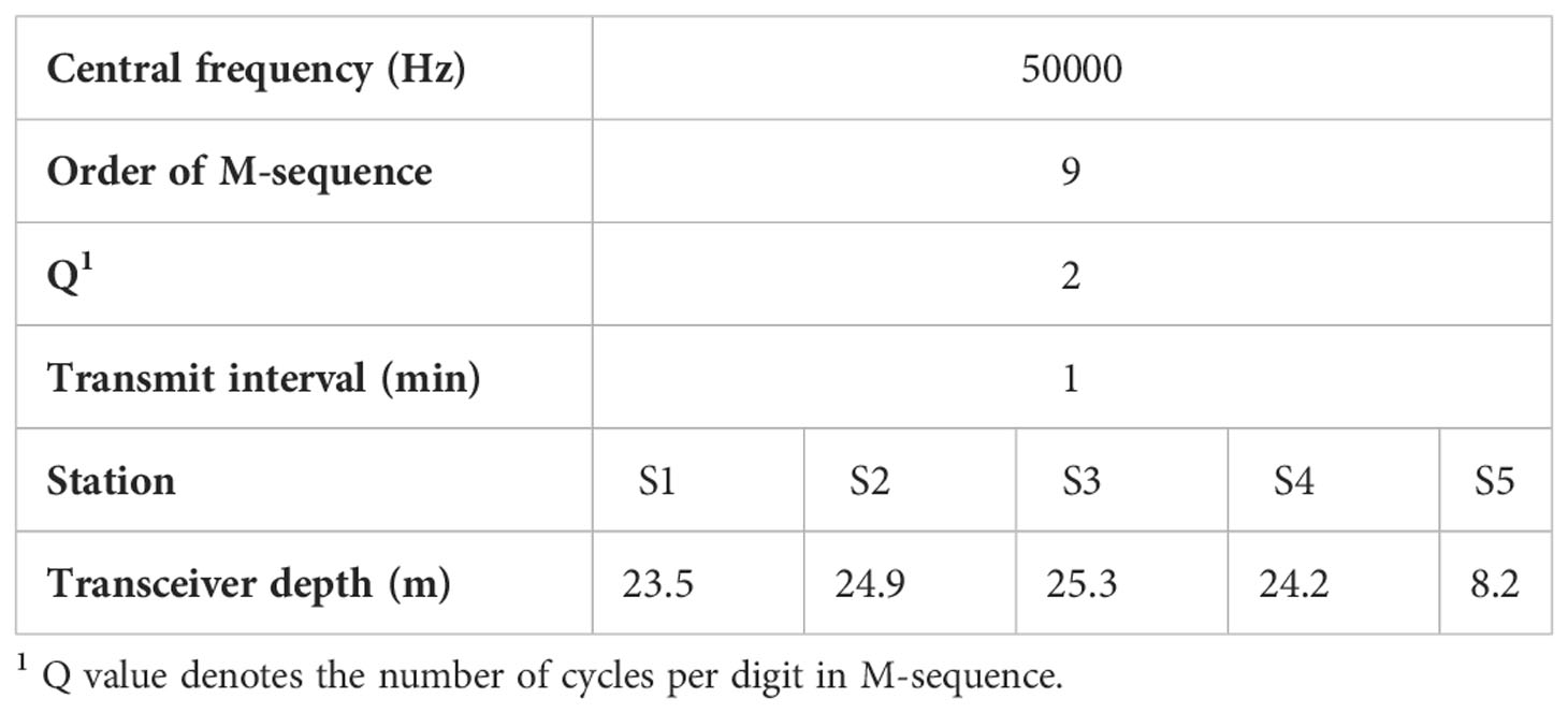
Table 1 Transmission signal and station parameters.

Due to the sensitivity of the high-frequency signal to the observation environment, undulate terrain and the station distance, the sound ray path structure is significantly fluctuated by the moving station. The terrain of experiment area (S1-S2, S2-S3, S3-S4 and S4-S1) were measured by depth gauge scanning. Unfortunately, S2 did not receive the acoustic signals because of the incorrect system setting, and the acoustic signal between S4 to S5 is mostly blocked due to the terrain. Therefore, in this paper, only the received data of S1to S5 and S3 to S5 are analyzed to simplify the processing of acoustic signals.

3 Methodology

In this section, the inversion problem and the Doppler shift effect are analyzed to reconstruct the flow current field by sound reciprocal transmission under relative motion condition. Ray simulation and multi-peak matching are also demonstrated.

3.1 Forward problem under relative motion condition

Reconstructing range-averaged sound speed and flow current velocity in the observation area by sound reciprocal travel time is the basic principle of CAT technology. Moving transceivers have relative velocity under the relative motion condition between sound station pairs (Xu et al., 2022). Figure 2 shows reciprocal sound signal transmission between relative motion station of S_i and S_j. Without loss of generality, the transmission mode is assumed with a uniform sound speed (C_m) and a uniform current velocity (U_m) in each grid of the unbounded medium. Two transceivers are moving with speeds V_I and V_J, the v_i and v_j are the projection of real speeds in the vertical of station pairs. The acoustic signals are sent and receipted simultaneously, where sound rays travel along sound paths connecting the station pairs. Thus, the reciprocal travel time of S_i and S_j are not only influenced by the environment (temperature, current, salinity), but also transceiver motion. Each sound ray travel time from S_i and S_j, t_ij, and the reversed direction, t_ji, can be expressed as follow:

FIGURE 2

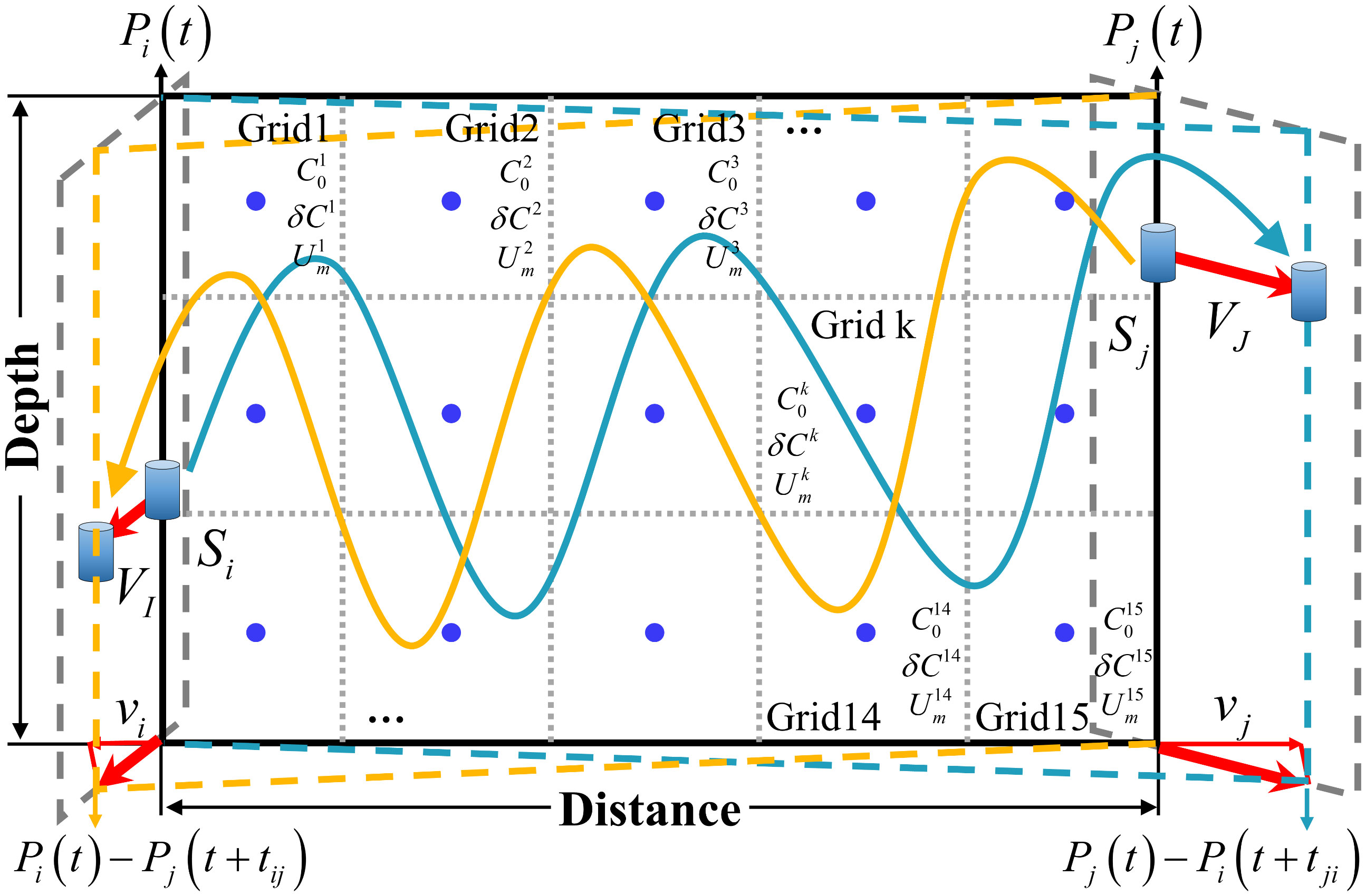
Figure 2 Reciprocal sound transmission between relative motion station S_i and S_j. Red arrows are the directions of station motion. The blue and yellow arrow lines denote the ray path and travel direction. The gray dotted lines are the grid division lines. The blue circles are the center point of girds for inversion calculation. Each grid assumes $C_0^k$, δC^k and $U_m^k$, respectively.

$\begin{array}{ll}\begin{array}{l}{t}_{ij}={\displaystyle {\int }_{{\Gamma }^{+}}\frac{ds}{C_m+U_m-v_j}\approx {\displaystyle \sum \frac{l_{ij}^k}{C_m^k+U_m^k-v_j}}}\\ t_{ji}={\displaystyle {\int }_{{\Gamma }^{-}}\frac{ds}{C_m+U_m-v_i}\approx {\displaystyle \sum \frac{l_{ij}^k}{C_m^k-U_m^k-v_j}}}\end{array}& (1)\end{array}$

where $l_{ij}^k$ is the length of sound ray pass through each gird in Figure 2. $C_m^k$ and $U_m^k$ are the grid-averaged sound speed and current, respectively. k is the grid number. The positive direction of v_i is away from the station j, similar with v_j.

By summing and subtracting the reciprocal transmission travel time in Eq. 1 with the reference travel time t₀, we obtained the travel time deviation (δt) and travel time difference (Δt):

$\begin{array}{ll}\begin{array}{l}\delta t=t_{ij}+t_{ji}-2t_0={\displaystyle \sum \left(\frac{l_{ij}^k}{C_m^k+U_m^k-v_j}+\frac{l_{ij}^k}{C_m^k-U_m^k-v_i}-2\frac{l_{ij}^k}{C_0^k}\right)}\\ \Delta t=t_{ij}-t_{ji}={\displaystyle \sum \left(\frac{l_{ij}^k}{C_m^k+U_m^k-v_j}-\frac{l_{ij}^k}{C_m^k-U_m^k-v_i}\right)}\end{array}& (2)\end{array}$

Simplifying the Eq. 2, uniform sound speed ($C_m^k$) in grid k decomposes into the sum of reference sound speed ($C_0^k$) and sound speed difference (δC^k).Both uniform current velocity ($U_m^k$<1m/s) and transceiver speed (v_i<1m/s) are far smaller than reference sound speed (about 1500m/s), the travel time deviation (δt) and travel time difference (Δt) can be simplified as Eq. 3 using Taylor expansions, the higher-order terms of Taylor expansion are omitted (Xu et al., 2021).

$\begin{array}{ll}\begin{array}{l}\delta t\approx -{\displaystyle \sum \left(\frac{l_{ij}^k\left(2\delta C^k-v_i-v_j\right)}{{\left(C_0^k\right)}^2}\right)}=-{\displaystyle \sum \frac{2l_{ij}^k}{{\left(C_0^k\right)}^2}\left(\delta C^k-\frac{v_i+v_j}{2}\right)}\\ \Delta t\approx -{\displaystyle \sum \left(\frac{l_{ij}^k\left(2U_m^k+v_i-v_j\right)}{{\left(C_0^k\right)}^2}\right)}=-{\displaystyle \sum \frac{2l_{ij}^k}{{\left(C_0^k\right)}^2}\left(U_m^k-\frac{v_j-v_i}{2}\right)}\end{array}& (3)\end{array}$

From the Eq. (3), δt is mainly influenced by δC^k and the sum of v_i and v_j, where δC^k is dominated by water temperature fluctuations about 0~1°C. Normally, δC^k is less than (v_i+v_j)/2. Δt is mainly influenced by $U_m^k$ and the sum of v_i and v_j, $U_m^k$ is larger than (v_i+v_j)/2. Meanwhile, the error of δt is caused by the position drift of acoustic station and the error of Δt is caused by the clock drift (Zhu et al., 2021). Thus, it can be summarized that the large error exists in solving of δt (water temperature). In other words, the underwater moving acoustic tomography is appropriate to solve Δt (water current velocity).

In this experiment, four moored acoustic station and one moving acoustic station are used. Comparing with the tidal current velocity at each moored station, the speeds of moored stations are considered to be close to zero, which can be neglected. Therefore, during the reciprocal transmission the speed of moving station S_j can represent the relative speed between moored station S_i and moving station S_j, i.e., v_i = 0. The S_j relative speed v_j is positive when the two stations move closer (S_j away from S_i). Thus, the travel time difference and the current speed U_m are expressed as Eq. 4.

$\begin{array}{ll}\Delta t=-{\displaystyle \sum \frac{2l_{ij}^k}{{\left(C_0^k\right)}^2}\left(U_m^k-\frac{v_j}{2}\right)}\Rightarrow U_m=-\frac{{\left(C_0\right)}^2}{2L_{ij}}\Delta t+\frac{v_j}{2}& (4)\end{array}$

where Δt is obtained by the sound transmission, C₀ is measured by CTD, L_ij is calculated by ray simulation and v_j is the travel speed of the boat using GPS. Eq. (4) can be expressed in a matrix form as:

$\begin{array}{ll}{\left[\begin{array}{c}\Delta t_1\\ \Delta t_2\\ ⋮\\ \Delta t_n\end{array}\right]}_{n\times 1}=-2{\left[\begin{array}{cccc}\frac{l_{ij}^{11}}{{\left(C_0^1\right)}^2}& \frac{l_{ij}^{12}}{{\left(C_0^2\right)}^2}& \cdots & \frac{l_{ij}^{1K}}{{\left(C_0^k\right)}^2}\\ \frac{l_{ij}^{21}}{{\left(C_0^1\right)}^2}& \frac{l_{ij}^{22}}{{\left(C_0^2\right)}^2}& \cdots & \frac{l_{ij}^{2K}}{{\left(C_0^k\right)}^2}\\ ⋮& ⋮& \ddots & ⋮\\ \frac{l_{ij}^{n1}}{{\left(C_0^1\right)}^2}& \frac{l_{ij}^{n2}}{{\left(C_0^2\right)}^2}& \cdots & \frac{l_{ij}^{nk}}{{\left(C_0^k\right)}^2}\end{array}\right]}_{n\times k}{\left[\begin{array}{c}{U}_m^1-\frac{v_j}{2}\\ U_m^2-\frac{v_j}{2}\\ ⋮\\ U_m^k-\frac{v_j}{2}\end{array}\right]}_{k\times 1}& (5)\end{array}$

where Eq. 5 represents the reciprocal transmission between a sound station pair. n is the number of sound ray paths, n = 1 corresponds to the 1st ray path. k is the number of girds, k = 1 corresponds to gird 1. $l_{ij}^{nk}$ represents the length of nth ray path in kth grid between S_i and S_j.

The inversion method, the ray simulation of motion station pair and the travel time identification are presented in the following. Besides, the approximate distance of station pair at clock t is denoted by P_i(t) – P_j(t). It should be noted that, due to the relative motion between S_i and S_j, the exact distance of the sound signal transmission from S_i to S_j is P_i(t) – P_j(t+t_ij) and S_j to S_i is P_j(t) – P_i(t+t_ji). The relative speed is much smaller than the sound speed, thus the error of the exact and the approximate distances can be ignored (Kaneko et al., 2020). However, the Doppler effort caused by the relative motion on the signal transmission need to be discussed, as shows in section 3.2.

3.2 Estimation and compensation of Doppler effect

The Doppler effect is caused by the motion of inhomogeneous water movement, such as: vehicle motions, surface waves, water turbulence, the relative motion of transceivers, etc. The time-varying effects of acoustic signal caused by Doppler effect in the water environment result in Doppler frequency shifts and additional frequency extensions. In this paper, for the underwater acoustic broadband transmission system, the Doppler effect is described by α (Doppler factor), which is defined as the ratio of the relative velocity V (v_j) between moored and moving transceivers to the sound speed C of observation area]. The Doppler factor is the ratio of frequency offset to signal frequency in the frequency domain as Eq. 7.

$\begin{array}{ll}\alpha =\frac{C}{V}=\frac{\Delta f}{f}& (6)\end{array}$

where Δf is the frequency offset and f is the carrier frequency of acoustic signal.

Compared to the rate of electromagnetic wave in wireless communication (3×10⁸ m/s), the sound wave in water is only about 1500m/s, where exists significant Doppler effect for moving signal transmission. Thus, the Doppler effect need to be estimated and compensated during the reciprocal signal transmission of transceivers’ relative motion.

The equivalent frequency of the moored station and moving station is different. If the receiving station (moving station S_j) is moving away from the sending station (moored station S_i) with speed v_j, for moving station, the travel time of one wavelength (λ) is t_v ≈ λ/(C+v_j) = (C/f)/(C+v_j), the equivalent frequency and Doppler frequency shift are as:

$\begin{array}{ll}\begin{array}{l}{f}_v=\frac{1}{t_v}=\frac{C+v_j}{C/f}=f\left(1+\frac{v_j}{C}\right)=f(1+\alpha )\\ \Delta f=f_v-f\approx f·\alpha \end{array}& (7)\end{array}$

For moored station, the received signal wavelength of moored station is compressed v_j/f, thus, equivalent signal wavelength is λ_v = λ–v_j/f = (C–v_j)/f, the equivalent frequency and Doppler frequency shift are as:

$\begin{array}{ll}\begin{array}{l}{f}_v=\frac{C}{{\lambda }_v}=\frac{C}{\left(C-v_j\right)/f}=f\left(\frac{1}{1-v_j/C}\right)=f\left(1+\frac{v_j}{C}+{\left(\frac{v_j}{C}\right)}^2···{\left(\frac{v_j}{C}\right)}^n\right)\approx f(1+\alpha )\\ \Delta f=f_v-f\approx f·\alpha \end{array}& (8)\end{array}$

During the experiment, if single-frequency acoustic signal was used. Received signal usually consists of multipath arrivals with different travel times that caused different Doppler frequency shifts in an underwater acoustic channel (Huang, 2019; Huang et al., 2019). As Eq. 7 and Eq. 8 shows, the moored station has same Doppler frequency shift with moving station. The received acoustic signal s(t) = e^jwt for multipath arrivals can be expressed as Eq. 9 when there is no Doppler frequency shift.

$\begin{array}{ll}y(t)=H(\omega ){\text{e}}^{jwt},\left(H(\omega )={\displaystyle \sum _{n=1}^N{A}_n}{\text{e}}^{-jw{\tau }_n}\right)& (9)\end{array}$

where n is the sound ray number, A_n and τ_n are the magnitude and travel time delay, respectively.

The received multipath signal with Doppler shift is express as follows:

$\begin{array}{ll}y(t)=H(\omega ,t){\text{e}}^{j\omega t}={\displaystyle \sum _{n=1}^N{A}_n}{\text{e}}^{-j\omega \left({\tau }_n-{\alpha }_{n}t\right)}{\text{e}}^{j\omega t}& (10)\end{array}$

It can be concluded that received signal is no longer a single-frequency signal and the transmission channel is time-varying. Therefore, non-consistent frequency received signal is compensated by resampling (Eq. 11), where basically eliminate the signal compression in time domain due to Doppler effect.

$\begin{array}{ll}{y}^{\prime }(t)=y\left(\frac{t}{1+\overline{\alpha }}\right)& (11)\end{array}$

It should be noted that the moving boat (moving station) was at a constant speed (0.6m/s) during the experiment, and the real-time positions were recorded by GPS. In post-processing, the direction and speed of moving station were established and plotted at each reciprocal signal transmission moment, as shown in Figures 3A, D. The Doppler effect ($\overline{\alpha }$) in Eq. 11 at each moment is calculated by this way. However, system still exist a deviation between computational and real solutions as Eq. 12 shows, which is small enough to be negligible.

FIGURE 3

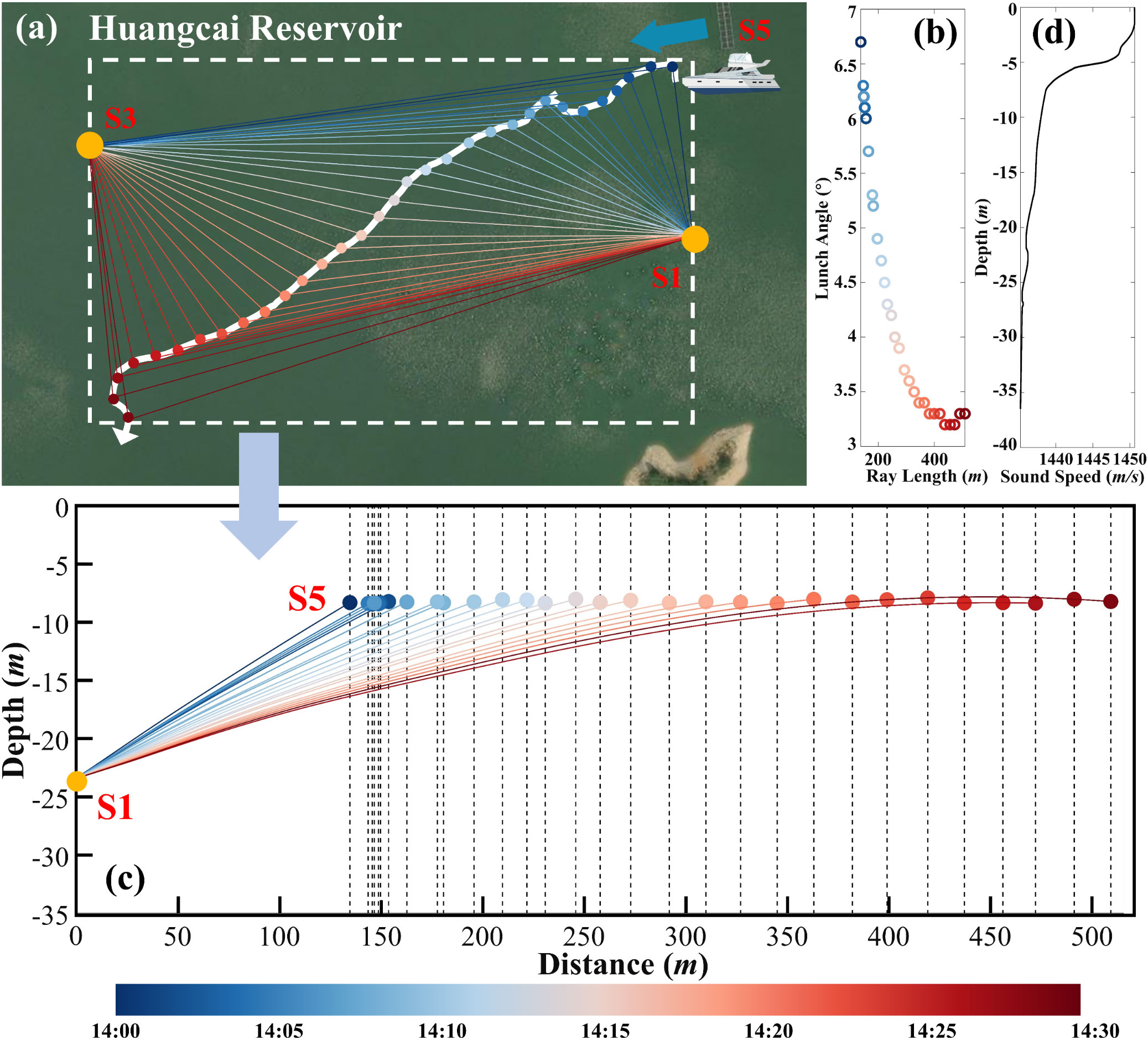
Figure 3 Reciprocal signal transmission during relative motion. (A) is the path of moving station at different moment. (B) is the relationship between launch angle and ray length. (C) is the ray simulation between station S1and S5 (Note that: only the direct rays are shown at (C). (D) is the sound speed profile in observation area. The color bar below shows the color of different moment.

$\begin{array}{ll}\ell =\frac{\alpha -\overline{\alpha }}{1+\overline{\alpha }}f& (12)\end{array}$

3.3 Inversion problem

The two-dimensional (2D) vertical depth-averaged flow current velocity can be calculated by the inverse method (Xu et al., 2021). Furthermore, three-dimensional (3D) current variations are reconstructed by multiple two-dimensional vertical current results through moving acoustic tomography model in a short period. Eq. 13 is the basic vertical solving matrix of S_i and S_j. The matrix expression is simplified to the following form:

$\begin{array}{ll}y=Ex+n& (13)\end{array}$

where y is the travel time difference data vector (y = {Δt_i}), E is the observation matrix ($E=-2\left\{l_{ij}^{nk}/{\left(C_0^k\right)}^2\right\}$) created by ray simulation, X is the unknown variable vector of current velocity ($X=U_m^k-\frac{v_j}{2}$), and n is the residual vector to measure the error terms.

The objective optimization function is defined as follows (Kaneko et al., 2020):

$\begin{array}{ll}J=(y-Ex{)}^T(y-Ex)+\lambda x^T{H}^{T}Hx& (14)\end{array}$

where H is a regularization matrix to smooth the grid solution by moving average of nearby grids. λ is the Lagrange multiplier to converge the results.

The expected solution is:

$\begin{array}{ll}\widehat{x}=(E^{T}E+\lambda H^{T}H{)}^{-1}{E}^{T}y& (15)\end{array}$

The λ in Eq. 14 and Eq. 15 is obtained when the residual defined is less than the predetermined error value. The inversion error $\widehat{n}$ and the iteration residual error ${\widehat{x}}_{err}$are expressed as:

$\begin{array}{ll}\widehat{n}=y-E\widehat{x}=\left\{I-E{\left(E^{T}E+\lambda H^{T}H\right)}^{-1}{E}^T\right\}y& (16)\end{array}$

$\begin{array}{ll}{\widehat{x}}_{err}={\left(E^{T}E+\lambda H^{T}H\right)}^{-1}{E}^T\widehat{n}& (17)\end{array}$

The grid-averaged current velocity in 2D vertical profile can be obtained via above process. Thus, 3D current field is reconstructed by the 2D current dataset at multiple moments.

3.4 Ray simulation and multi-peak matching

Ray simulation is used as a post-processing simulation to identify the multi-peak of received acoustic signal, E in Eq. 13 is formed by grid divided of ray structure after matching multi-peaks. In typical acoustic tomography experiments, all acoustic stations are fixed, and it only needs to use the obtained terrain for ray simulation between the station pairs. However, in this experiment, the ray structure is changing due to the varying terrain with moving station and the time-varying channel by Doppler effect.

The obtained resampled signal results after correlation in Figure 4 show that the peak is not very obvious. The red circles in top of Figure 4 are the identified peaks by matching with ray simulations. The process of peak identification has followed steps: acoustic signals are resampled as method in part 4.2 before correlation; the station distances at each moment are obtained by GPS recording between moving and moored station; the arrival signals are identified and matched with the largest SNR value peaks in the reference travel time window (obtained by station distances). Also, ray simulations at different distance are conducted to match peaks in receiving signals. Figures 3B, C show the relationship between launch angle with ray length and ray simulation results of S1 to S5, respectively. The sound ray structure stacked diagram (Figure 4C) is the simulation at different station distance based on sound speed profile measured by CTD.

FIGURE 4

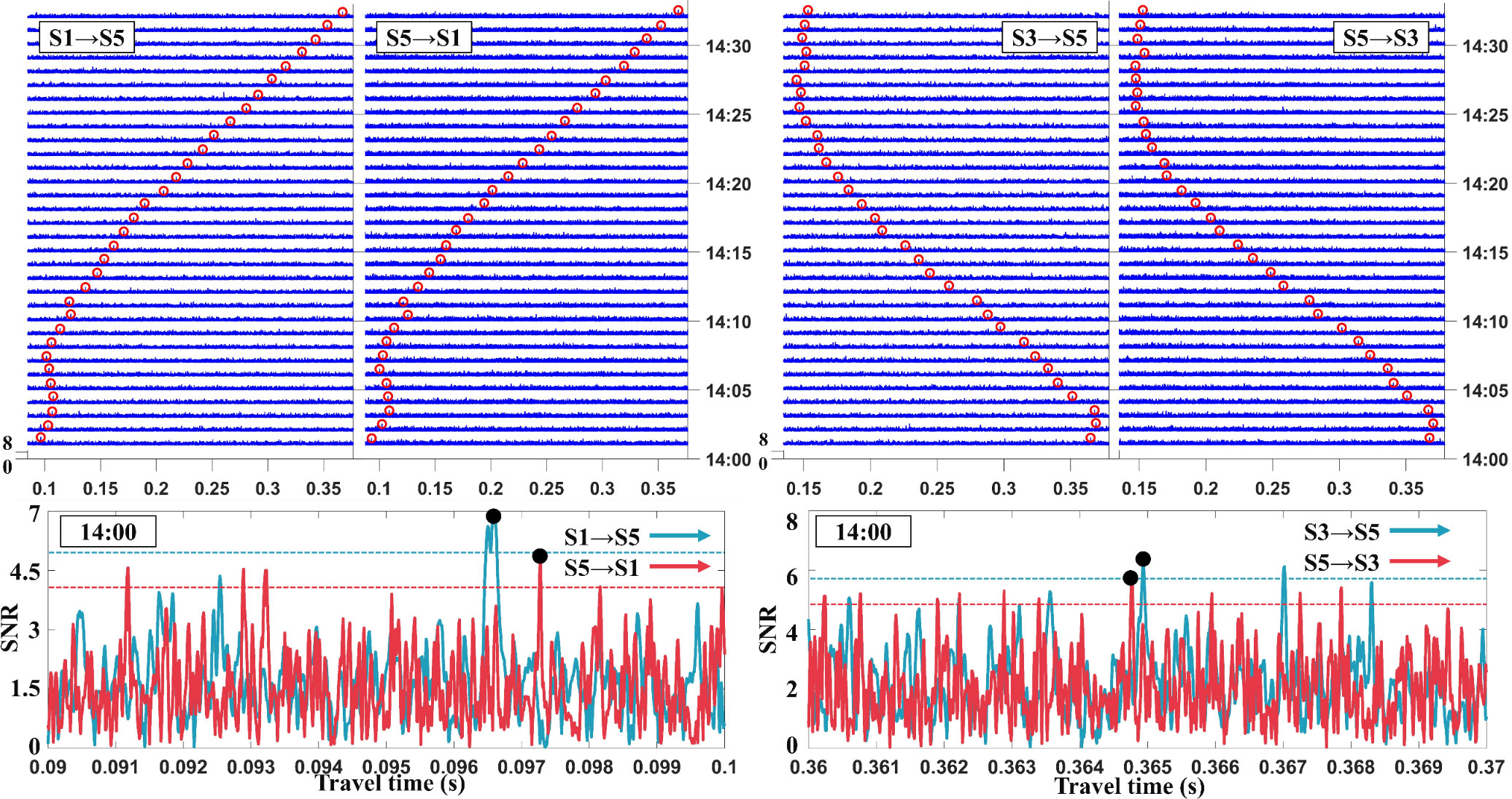
Figure 4 Correlation results of resampled signal (S1-S5 and S3-S5). The upper four figures are correlation results from 14:00 to 14:32. The abscissa axis above denotes the travel time of acoustic signal; ordinate axis denotes the date time of sending signals; the peaks’ height denotes SNR value; and the red circles denote the identified peaks. The lower two figures are the reciprocal transmission patterns of S1-S5 and S3-S5, respectively. Red and blue dotted lines are the divide lines for high SNR.

The reciprocal resampled acoustic signals after correlation at 14:00 are shown in Figure 4 blow, where the results have significant multi ray path. Due to uncertainty of terrain caused by the moving stations, the multipath cannot be matched with ray simulation, and only the direct ray was simulated and identified. In addition, the low SNR values show that the Doppler effect caused by the moving station has a significant influence on signal attenuation. It should be noted that the sound speed profile is a negative gradient and has been introduced in the article (Xu et al., 2022).

In the inversion calculation, the vertical profiles of sound station pairs are used as gridded slice method in 2D (Xu et al., 2021). As only the direct ray was used, the horizontal stratification lines were set at 6m and 26m and the vertical stratification was divided into four layers evenly. The inverse results of the current field for a total of four grids at this layer were solved. The division method is designed to ensure that the ray length in each grid is close to reduce the inversion error.

4 Results

4.1 Travel time differences

Figure 5 shows the variations of travel time and travel time differences of direct arrival rays of S1 to S5 and S3 to S5, respectively. As shown in Figure 5, the variation trends of reciprocal transmissions at each station pair are basically the same. The travel time difference (TTD) calculated as Eq. 2 is the fluctuate obviously which corresponds to the current changing. The mean and standard travel time differences are displayed in Table 2. The mean travel time difference of S1-S5 is significantly higher than S3-S5, which means the flow current variations along S1-S5 path are stronger.

FIGURE 5

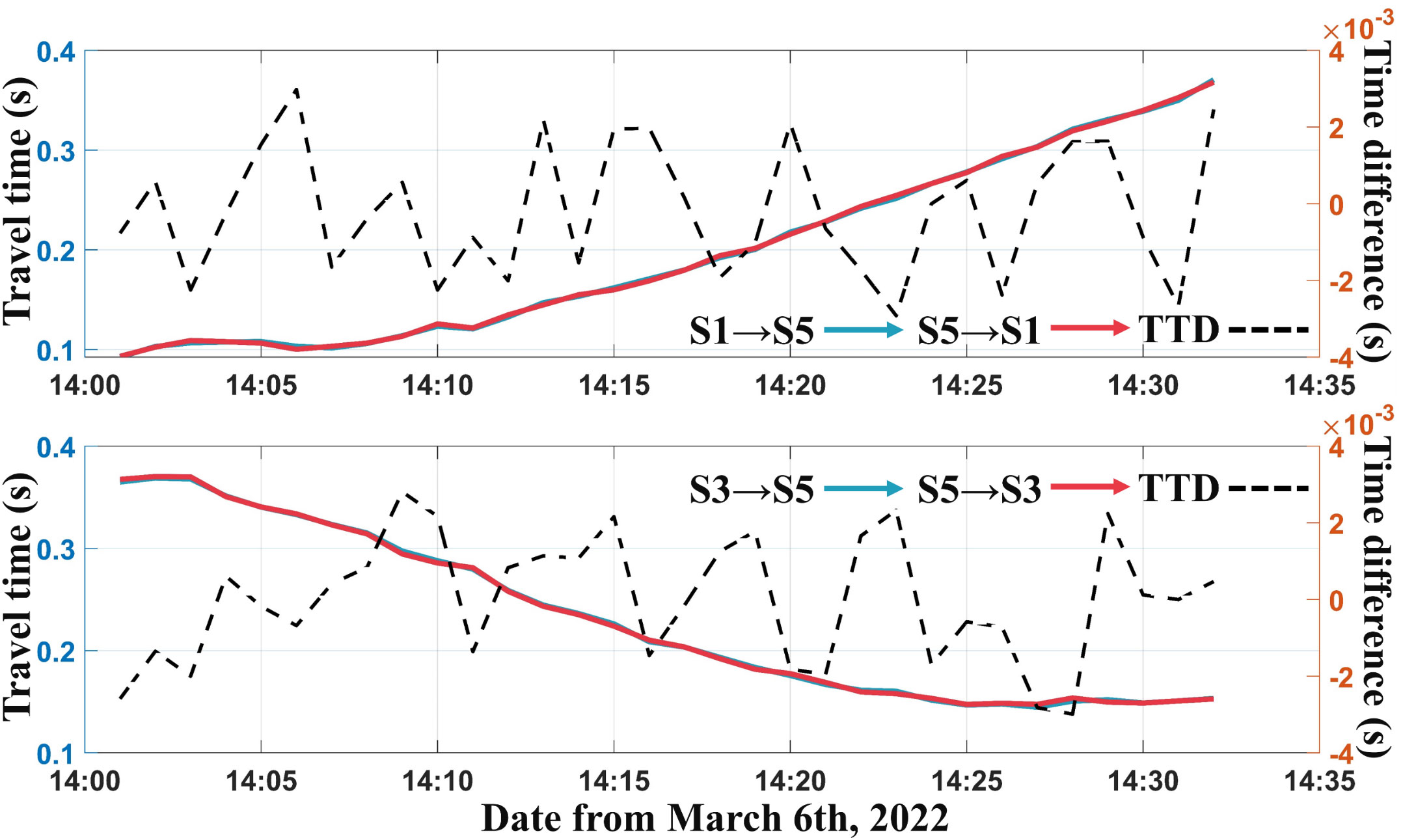
Figure 5 Travel time and travel time differences. Left axis is the range of travel time and right axis is the range of travel time differences.

TABLE 2

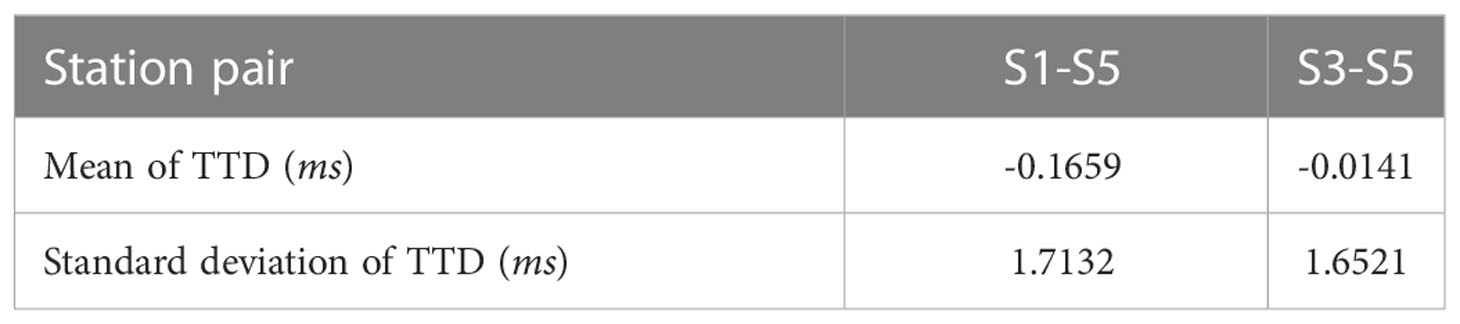
Table 2 Mean and standard deviation of travel time differences.

4.2 Inversion result

The layer-averaged flow current velocity of S1 to S5 and S3 to S5 are shown at Figures 6A, B, respectively. The result of layer-averaged current is the mean of all grid central point inversion results at same depth. The red lines display the current fluctuations and blue lines are the inversion results using 5-minute moving average. The moving average reduces the effect of anomalies and retains more information on variations through weighted distribution, which makes current trends more visible.

FIGURE 6

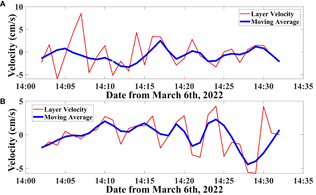
Figure 6 Inversion results of layer-averaged current. (A) is the layer-averaged current of S1 to S5. (B) is the layer-averaged current of S3 to S5. Red lines are the variations of inversion current results real-time at depth of 16m, and blues are the moving average of red lines.

From Figure 6, variations of the layer-averaged current in the vertical profile is about -5 to 5 cm/s, positive and negative represent the direction of current (the pre-set range-layer error before inversion is 0.01m/s, and the inversion error is much smaller than the pre-set value). Although the current at this layer is not strong, the direction of current varies quickly. The variability of directions in the layer-averaged currents is caused by the turbulence current in the reservoir. The inversion method for average current ignores the current in the vertical direction, which normalises the changing of current via travel time differences in certain depth lines (layer-averaged method) or grid points (grid-averaged method).

Figure 7A is a 3D combination figure of flow current velocity and direction at each grid in vertical profiles. It shows the inversion current field results via the moving station at different locations. All 2D vertical profiles have four grid-averaged results at depth of 16m. Figures 7B-G is the 2D horizontal flow fields. The Figure 6 indicates the convergence results of inversion current field over a 30-minute observation period. The current along vertical profiles vary about 5-minute interval of each station pair. But the results of horizontal flow fields show the current directions is basically unchanged. It is speculated that the flow field is stability, but a small-scale dynamic progress and water exchange exist in observation area. However, only the matched direct ray paths are used for inversion, where more accurate changing of current field cannot be identified.

FIGURE 7

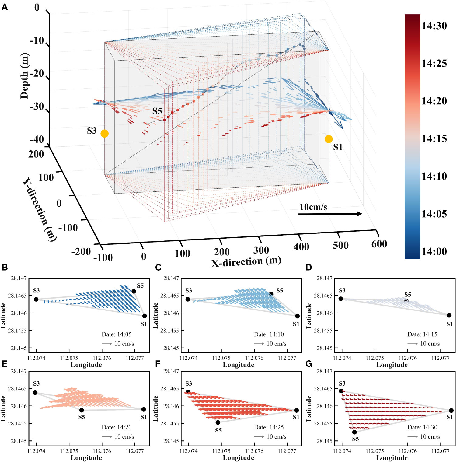
Figure 7 Inversion results of current field. (A) is the 3D combination figure. Different colour denotes different profile that same as the position at Figure 3. The arrows denote the velocity and direction of flow current at each grid. The grey area is critical observation area. (B–G) is the horizontal flow fields at six moments.

5 Discussion

Underwater moving acoustic tomography is an enhancement and application of CAT technique. It combines the traditional observation with the motion observation technique to cover the entire spatial area. By reconstructing 2D layer-averaged results and 3D spatial distribution in a feasibility experiment at Huangcai Reservoir, the method has been basically proved to facilitate the observation of current field.

The advantage of moving acoustic tomography compared with traditional observation via fixed stations is that the moving stations can compensate for areas of that sound ray in fixed observation do not pass through, reconstructing the environment variation over the whole area. However, the disadvantage of this technique is the drift and multipath uncertainty of reciprocal acoustic signals caused by Doppler effect and terrain variations. For example, in this paper, the experiment was carried out with four moored stations and one moving station, but due to the terrain and signal, only two moored stations and one moving station were effectively communicated with each other. Further, although recovering correlation signal via resampling techniques in moving acoustic tomography is initially proposed in this paper, the resolution of multipath identification is still a challenge (especially in shallow areas).

In addition, the 3D current results in 4.2 are reconstructed using grid-averaged current in vertical profile, instead of using stream function to create 2D current field (Syamsudin et al., 2016; Zhu et al., 2017a; Zhu et al., 2017b; Syamsudin et al., 2019). This approach is faster and more intuitive, but is unable to characterise the variation of current along vertical direction. This experiment used only three stations to reconstruct the current field, the errors in final results still exists. It is believed that the observation data and inversion results can be more accurate with more station reciprocal transmission data.

Huang et.al is the first developed moving acoustic tomography and applied in ocean flow field observation. The main differences between ours and theirs are the experiment scale and signal processing method. On the one hand, we used 50kHz transceiver for high precision moving tomography in a small-scale area and they used 18k transceiver in long-range (15km) observation. On the other hand, we resampled the signal to correct the signal travel time, while they corrected the arrival travel time via Doppler compensation. The inversion results have higher accuracy after high frequency transmission and signal resampled.

Moving acoustic tomography is more suitable for phenomena with slow fluctuations of current velocity and is not applicable to phenomena with temperature or quick variations of current. The method can be implemented similarly to a large long baseline array observation, where an accurate 3D environmental field is constructed by moving stations to observe the entire environment region.

To conclude, combining experiments and data analysis, the following empirical applications are given: moving acoustic tomography is more suitable for shallow areas with slow terrain fluctuations; using higher frequency signals (>3k) to obtain effective multipath sound structure; controlling the distance between moving and moored stations to reduce the signal travel time drift by the Doppler effect.

6 Conclusion

Underwater environment observation via advanced acoustic tomography has been considerably developed in recent years. In this paper, a method for reconstructing 3D layer-averaged flow current fields using high-frequency acoustic signal via short-term moving tomography is developed. The study introduces the basic idea of resampling acoustic signal and the calculation method for obtaining flow current. 3D flow current field result is composed by grid-averaged inversion current of vertical profile via moving station at different moment. Thus, a moving CAT observation experiment was carried out at range of 500m×500m in a reservoir to verify the feasibility of underwater moving acoustic tomography. The received results of reciprocal signal transmission between two moored stations and one moving station were used for layer-averaged current variations at vertical scale and grid-averaged current. The feasibility of the method is proved and its applicability is discussed.

The main conclusions of this research are as follows:

1. Underwater moving acoustic tomography can be used to complement areas that traditional fixed acoustic stations cannot observe and fuse the observation data. Experiments have initially proved the feasibility of this idea and the reliability of the inversion method process.

2. The acoustic signal needs to be re-sampled and correlated as the moving stations brings Doppler effect on the signal transmission. Particularly in shallow areas, the effect of real time variations in terrain causes signals difficult to be identified and matched. It is a problem that needs to be further analysed.

3. Moving acoustic tomography can be used in 3D observations. Rather than range averaging acoustic information over the path of sound rays passing in 2D planes, moving tomography is able to fuse 2D data to perceive and acquire 3D spatial observation, which has high application value.

The application of underwater moving acoustic tomography and signal processing via multiple stations in the ocean will be the focus of our future work. Data assimilation in 3D flow current field structures is also a research topic.

Data availability statement

The original contributions presented in the study are included in the article/supplementary material. Further inquiries can be directed to the corresponding authors.

Author contributions

SX: Experimentation, methodology, formal analysis, data curation, investigation, validation, writing original draft, reviewing and editing. GL: Conceptualization, experimentation, formal analysis, data curation, validation, reviewing and Editing. RF: formal analysis, data curation, reviewing and editing. ZH and PX: supervision, validation, reviewing and editing. HH: Conceptualization, funding acquisition, project administration, supervision, reviewing and editing. All authors contributed to the article and approved the submitted version.

Funding

This work was supported by the National Natural Science Foundation of China (grant number 52071293).

Acknowledgments

We thank our colleagues in National University of Defense Technology for their experimental platform support and access to the experiment field sites. The raw data obtained from small-scale CAT system TD, CTD would be available upon request through Haocai Huang at Zhejiang University (hchuang@zju.edu.cn).

Conflict of interest

The authors declare that the research was conducted in the absence of any commercial or financial relationships that could be construed as a potential conflict of interest.

Publisher’s note

All claims expressed in this article are solely those of the authors and do not necessarily represent those of their affiliated organizations, or those of the publisher, the editors and the reviewers. Any product that may be evaluated in this article, or claim that may be made by its manufacturer, is not guaranteed or endorsed by the publisher.

References

Al Sawaf M. B., Kawanisi K. (2018). Novel high-frequency acoustic monitoring of streamflow-turbidity dynamics in a gravel-bed river during artificial dam flush. Catena 172, 738–752. doi: 10.1016/j.catena.2018.09.033

CrossRef Full Text | Google Scholar

Al Sawaf M. B., Kawanisi K., Kagami J., Bahreinimotlagh M., Danial M. M. (2017). Scaling characteristics of mountainous river flow fluctuations determined using a shallow-water acoustic tomography system. Physica A: Stat. Mech its Appl 484, 11–20. doi: 10.1016/j.physa.2017.04.168

CrossRef Full Text | Google Scholar

Bahreinimotlagh M., Kawanisi K., Al Sawaf M. B., Roozbahani R., Eftekhari M., Khoshuie A. K. (2019). Continuous streamflow monitoring in shared watersheds using advanced underwater acoustic tomography system: a case study on zayanderud river. Environ. Monit. Assess 191 (11), 1–9. doi: 10.1007/s10661-019-7830-4

CrossRef Full Text | Google Scholar

Bahreinimotlagh M., Kawanisi K., Danial M. M., Al Sawaf M. B., Kagami J. (2016). Application of shallow-water acoustic tomography to measure flow direction and river discharge. Flow Meas Instrum 51, 30–39. doi: 10.1016/j.flowmeasinst.2016.08.010

CrossRef Full Text | Google Scholar

Chen M., Hanifa A. D., Taniguchi N., Mutsuda H., Zhu X., Zhu Z., et al. (2022). Coastal acoustic tomography of the neko-seto channel with a focus on the generation of nonlinear tidal currents–revisiting the first experiment. Remote Sens 14 (7), 1699. doi: 10.3390/rs14071699

CrossRef Full Text | Google Scholar

Chen K., Huang C.-F., Huang S.-W., Liu J.-Y., Guo J. (2020). Mapping coastal circulations using moving vehicle acoustic tomography. J. Acoust Soc. America 148 (4), EL353–EL358. doi: 10.1121/10.0002031

CrossRef Full Text | Google Scholar

Chen M., Kaneko A., Lin J., Zhang C. (2017). Mapping of a typhoon-driven coastal upwelling by assimilating coastal acoustic tomography data. J. Geophys Res: Ocean 122 (10), 7822–7837. doi: 10.1002/2017jc012812

CrossRef Full Text | Google Scholar

Chen M., Kaneko A., Zhang C., Lin J. (2016). 3D assimilation of Hiroshima bay acoustic tomography data into a Princeton ocean circulation model. J. Acoust Soc. America 140 (4), 3183–3183. doi: 10.1121/1.4970008

CrossRef Full Text | Google Scholar

Chen M., Syamsudin F., Kaneko A., Gohda N., Howe B. M., Mutsuda H., et al. (2020). Real-time offshore coastal acoustic tomography enabled with mirror-transpond functionality. IEEE J. Ocean Eng 45 (2), 645–655. doi: 10.1109/joe.2018.2878260

CrossRef Full Text | Google Scholar

Chen C., Yang K., Ma Y. (2019). Sensitivity of sound speed fluctuation on acoustic arrival delay of middle range in deep water. Appl. Acoust 149, 68–73. doi: 10.1016/j.apacoust.2019.01.020

CrossRef Full Text | Google Scholar

Chen Z., Zheng H., Tang Y., Chen C. (2021). Measurement of Yangtze river flow based on coastal acoustic tomography. J. Phys: Conf. Ser 1739 (1), 012032. doi: 10.1088/1742-6596/1739/1/012032

CrossRef Full Text | Google Scholar

Chen M., Zhu Z., Zhang C., Zhu X., Liu Z., Kaneko A. (2021). Observation of internal tides in the qiongzhou strait by coastal acoustic tomography. J. Ocean Univ. China 20 (5), 1037–1045. doi: 10.1007/s11802-021-4590-x

CrossRef Full Text | Google Scholar

Chen M., Zhu Z.-N., Zhang C., Zhu X.-H., Wang M., Fan X., et al. (2020). Mapping current fields in a bay using a coast-fitting tomographic inversion. Sensors 20 (2), 558. doi: 10.3390/s20020558

PubMed Abstract | CrossRef Full Text | Google Scholar

Huang C.-F. (2019). The development of acoustic mapping of ocean currents in coastal seas. J. Acoust Soc. America 146 (4), 2808–2808. doi: 10.1121/1.5136728

CrossRef Full Text | Google Scholar

Huang C. F., Li Y. W., Taniguchi N. (2019). Mapping of ocean currents in shallow water using moving ship acoustic tomography. J. Acoust Soc. America 145 (2), 858–868. doi: 10.1121/1.5090496

CrossRef Full Text | Google Scholar

Huang H., Xu S., Xie X., Guo Y., Meng L., Li G. (2021). Continuous sensing of water temperature in a reservoir with grid inversion method based on acoustic tomography system. Remote Sens 13 (13), 2633. doi: 10.3390/rs13132633

CrossRef Full Text | Google Scholar

Kaneko A., Zhu X. H., Lin J. (2020). Coastal acoustic tomography (Amsterdam: Elsevier Science Bv), WOS:000616677100016.

Google Scholar

Kawanisi K., Bahrainimotlagh M., Al Sawaf M. B., Razaz M. (2016). High-frequency streamflow acquisition and bed level/flow angle estimates in a mountainous river using shallow-water acoustic tomography. Hydrol Process 30 (13), 2247–2254. doi: 10.1002/hyp.10796

CrossRef Full Text | Google Scholar

Mohamad Basel Al S., Kiyosi K., Cong X., Gillang Noor Nugrahaning G., Faruq K. (2022). Monitoring inflow dynamics in a multipurpose dam based on travel-time principle. Water Resour. Manage, 1–22. doi: 10.1007/s11269-022-03161-w

CrossRef Full Text | Google Scholar

Munk W., Wunsch C. (1979). Ocean acoustic tomography - scheme for Large-scale monitoring. Deep-Sea Res. Part a-Oceanogr Res. Pap 26 (2), 123–161. doi: 10.1016/0198-0149(79)90073-6

CrossRef Full Text | Google Scholar

Syamsudin F., Adityawarman Y., Sulistyowati R., Sutedjo B., Kaneko A., Goda N. (2016). Applicability and feasibility studies of coastal acoustic tomography for long-term monitoring of the Indonesian throughflow transport variability. J. Acoust Soc. America 140 (4), 3076–3076. doi: 10.1121/1.4969586

CrossRef Full Text | Google Scholar

Syamsudin F., Taniguchi N., Zhang C., Hanifa A. D., Li G., Chen M., et al. (2019). Observing internal solitary waves in the lombok strait by coastal acoustic tomography. Geophys Res. Lett 46 (17-18), 10475–10483. doi: 10.1029/2019gl084595

CrossRef Full Text | Google Scholar

Xiao C., Kawanisi K., Torigoe R., Al Sawaf M. B. (2021). Mapping tidal current and salinity at a shallow tidal channel junction using the fluvial acoustic tomography system. Estuar Coast. Shelf Sci 258, 107440. doi: 10.1016/j.ecss.2021.107440

CrossRef Full Text | Google Scholar

Xu S., Li G., Feng R., Hu Z., Xu P., Huang H. (2022). Tomographic mapping of water temperature and current in a reservoir by trust-region method based on CAT. IEEE Trans. Geosci. Remote Sens 60, 1–14. doi: 10.1109/TGRS.2022.3220648

CrossRef Full Text | Google Scholar

Xu S., Xue Z., Xie X., Huang H., Li G. (2021). Ayer-averaged water temperature sensing in a lake by acoustic tomography with a focus on the inversion stratification mechanism. Sensors 21 (22), 7448. doi: 10.3390/s21227448

PubMed Abstract | CrossRef Full Text | Google Scholar

Zhu Z.-N., Zhu X.-H., Guo X. (2017a). Coastal tomographic mapping of nonlinear tidal currents and residual currents. Cont Shelf Res 143, 219–227. doi: 10.1016/j.csr.2016.06.014

CrossRef Full Text | Google Scholar

Zhu Z. N., Zhu X. H., Guo X., Fan X., Zhang C. (2017b). Assimilation of coastal acoustic tomography data using an unstructured triangular grid ocean model for water with complex coastlines and islands. J. Geophys Res: Ocean 122 (9), 7013–7030. doi: 10.1002/2017jc012715

CrossRef Full Text | Google Scholar

Zhu Z.-N., Zhu X.-H., Zhang C., Chen M., Zheng H., Zhang Z., et al. (2021). Monitoring of Yangtze river discharge at datong hydrometric station using acoustic tomography technology. Front. Earth Sci 9, 723123. doi: 10.3389/feart.2021.723123

CrossRef Full Text | Google Scholar