Evaluating historic and modern optical techniques for monitoring phytoplankton biomass in the Atlantic Ocean

1 Introduction

Phytoplankton play a central role in the Earth System, contributing to around half the world’s organic carbon and oxygen production (Longhurst et al., 1995; Field et al., 1998). They act as a conduit for propagating solar energy into the marine ecosystem, supporting marine life and sustaining fisheries (Chassot et al., 2010). They are intimately linked to the biogeochemical cycles of many key elements and compounds in the ocean, helping to regulate the climate of our planet (Falkowski, 2012).

Climate change is considered one of the greatest threats to life on Earth (Dow and Downing, 2011). Sea surface temperatures are rising, sea-level increasing, parts of the ocean are becoming more stratified, oxygen minimum zones are expanding, and the oceans are becoming more acidic (IPCC, 2019), with consequences for marine life. While many studies have investigated the impact of climate variability and change on marine phytoplankton (e.g., Behrenfeld et al., 2006; Martinez et al., 2009; Boyce et al., 2010; Wernand and van der Woerd, 2010a; Behrenfeld, 2011; Boyce et al., 2012; Brewin et al., 2012b; Wernand et al., 2013b; Behrenfeld, 2014; Boyce et al., 2014; Dutkiewicz et al., 2019; Henson et al., 2021) results are not always in agreement, with differences thought to be related to variations in the methods used for data collection, differences in data processing, and dealing with spatial and temporal biases in data collection (Gregg and Conkright, 2002; Antoine et al., 2005; Boyce et al., 2010; Mackas, 2011; McQuatters-Gollop et al., 2011; Rykaczewski and Dunne, 2011; Wernand et al., 2013b; Raitsos et al., 2014).

Phytoplankton may respond to climate change in different ways. For example, through changes in community composition, phenology, metabolic rates, geographical distribution, and vertical structure (Sathyendranath et al., 2017; Brewin et al., 2022) to name a few. Arguably one of the most important metrics to monitor is phytoplankton biomass, considering this metric is explicitly linked to many of these responses. Though not a perfect measure of phytoplankton biomass, since it can change independently through processes like photo-acclimation, the total chlorophyll-a concentration (Chl-a) is one of the most commonly-used metrics of phytoplankton biomass, owing to the fact it is present in all of phytoplankton (in one form or another), is relatively easy to measure (both in situ (directly and visually) and remotely (e.g., satellite)) at a sufficient accuracy and precision, with data being available over long periods needed to monitor change. Consequently, the Global Climate Observing System programme (GCOS) consider Chl-a to be an Essential Climate Variable (GCOS, 2011).

A key requirement for monitoring the response of phytoplankton biomass to climate change is to have a global dataset of a sufficient length to separate anthropogenic climate change from natural climate variability (e.g., >40 years in length; Henson et al., 2010). Though it is clear that satellites will become the main source of data used in the future for monitoring the response of phytoplankton to climate change (e.g., Siegel and Franz, 2010; Sathyendranath et al., 2019), the continuous ocean-colour data record is not yet at a sufficient length to do so. Ocean robotic platforms are increasing in number (Chai et al., 2020) and can measure deeper into the water column than the satellites, but have only been operating widely for a few decades. Time-series stations are critical (Henson, 2014), and in some cases have data available for >40 years (e.g., Bermuda Atlantic Time-series Study (BATS), Hawaii Ocean Time-series (HOT), Stončica), but are only available at discrete locations. At present, our only means to understand the global response of phytoplankton to climate change, at appropriate time scales (e.g., centennial), is to bridge modern measurements of Chl-a with historic proxies estimated by visual means, such as those collected using a Secchi disk, Forel-Ule colour scale, or the Continuous Plankton Recorder’s (CPR) phytoplankton colour index (Lewis et al., 1988; Falkowski and Wilson, 1992; Boyce et al., 2010; Wernand et al., 2013b; Raitsos et al., 2014).

Among the oldest instruments used in optical oceanography are the Secchi disk (Secchi, 1864) and Forel-Ule colour scale (Forel, 1890; Ule, 1892). A Secchi disk is a white (typically) disk one lowers into the water and the depth at which it disappears/reappears from sight is proportional to water clarity or transparency (Tyler, 1968; Preisendorfer, 1986; Wernand, 2010; Wernand and Gieskes, 2012; Pitarch, 2020). The Forel-Ule colour scale is a visual scale of 21 colours, ranging from blue to green to yellow to brown, that can be used alongside the Secchi disk with the observer typically recording the colour of a submerged Secchi disk at around roughly half the Secchi depth (Wernand and Gieskes, 2012). This visual index of colour can reflect information on the composition of optically active constituents in the water, such as sediment, phytoplankton and yellow substances (Wernand and van der Woerd, 2010b; Wang et al., 2019; Ye and Sun, 2022). In open-ocean case-1 waters (around 70% of the ocean surface; Hu et al., 2012), where optically active water constituents covary in a predictable manner with phytoplankton (Morel and Prieur, 1977), these visual indices can be a powerful predictor of Chl-a concentration (Boyce et al., 2010). In case-2 waters, where optically active water constituents do not covary in a predictable manner with phytoplankton (Morel and Prieur, 1977), relating Secchi depth and Forel-Ule colour readings to a Chl-a concentration can be more challenging.

In open-ocean case-1 waters, converting Secchi depth and Forel-Ule readings to a Chl-a concentration typically requires establishing statistical, empirical or analytical relationships (Boyce et al., 2012; Lee et al., 2015; Lee et al., 2018c). When searching for long-term trends, it is essential to quantify the accuracy of these conversions and their uncertainties (Boyce et al., 2012; Boyce et al., 2014), to minimise systematic biases between methods (Rykaczewski and Dunne, 2011), and to bridge these historic datasets with modern radiometric measurements used to derive Chl-a, considering satellite radiometry will soon become the main source of data for monitoring the impact of climate change on phytoplankton (Siegel and Franz, 2010; Wernand et al., 2013a; Lee et al., 2018b; Pitarch et al., 2019; Sathyendranath et al., 2019; Pitarch et al., 2021). To achieve these requirements, a comprehensive, consistent, co-located in-situ dataset of Secchi depth, Forel-Ule colour, Chl-a concentration and radiometric measurements is required, that covers the range of conditions representative of open-ocean waters. At present, the distribution of in-situ data available is biased toward coastal and eutrophic waters, with few measurements collected in the less accessible open-ocean (Brewin et al., 2016; Lee et al., 2018a)

The Atlantic Meridional Transect (AMT) is an open-ocean research programme that collects oceanographic data through the centre of the Atlantic Ocean, across a transect of >12,000 km, covering shelf seas and upwelling systems, and the mid-ocean oligotrophic gyres (Aiken et al., 2000; Robinson et al., 2006; Rees et al., 2017). The programme has been operating since 1995, with 29 cruises completed to date. Additional details of the AMT programme can be found on the AMT website (https://amt-uk.org). Among the current objectives of AMT, there is a requirement to construct a multi-decadal, multidisciplinary ocean time-series, and to provide essential sea-truth validation for current and next-generation satellite missions (Rees et al., 2015). In-line with these two objectives, and with a view towards using AMT data to help toward constructing time-series data of phytoplankton at a length longer than that collected during the programme, we collected a dataset of concurrent and co-located measurements of Secchi depth, Forel-Ule colour, Chl-a, hyperspectral remote-sensing reflectance (R_rs), diffuse attenuation (K_d) and beam attenuation (c), on four AMT cruises (AMTs 23, 25, 26 and 28, a total of 127 stations). In this paper, we use this dataset to evaluate techniques that convert Secchi depth, Forel-Ule colour and R_rs data to measurements of Chl-a, that have been used for constructing centennial scale time-series data on phytoplankton biomass, and to evaluate satellite algorithms designed to monitor these variables.

2 Methods

2.1 Statistical tests

To compare variables, we used the Pearson linear correlation coefficient (r), the squared Pearson linear correlation coefficient (r²), the centre-patterned (or unbiased) root mean square difference (Δ) and the bias (δ). The latter two statistics representing an index of precision and accuracy of a model, respectively. The root mean square difference ($\text{Ψ}$), which contains information on both accuracy and precision, can be reconstructed from Δ and δ, according to, $\text{Ψ}=\sqrt{{\text{Δ}}^2+{\mathit{\delta }}^2}$. The value of Δ and δ were computed according to

$\begin{array}{ll}\text{Δ}={\left(\frac{1}{N}\sum _{i=1}^N{\left\{[X_{i,1}-\left(\frac{1}{N}\sum _{j=1}^N{X}_{j,1}\right)]-[X_{i,2}-\left(\frac{1}{N}\sum _{k=1}^N{X}_{k,2}\right)]\right\}}^2\right)}^{1/2},& (1)\end{array}$

$\begin{array}{ll}\delta =\frac{1}{N}\sum _{i=1}^N(X_{i,1}-X_{i,2}),& (2)\end{array}$

where X is the variable and N is the number of samples. The subscripts 1 and 2 represent different estimates of the same variable, with 1 typically representing the estimated variable and 2 the measured variable. In many cases, statistical tests were performed in log₁₀ space, depending on whether the distribution of the data was closer to log-normal. Linear models relating two variables (e.g., Secchi depth and Chl-a) were fitted (often after log₁₀-transformation of one or both variables, depending on their distribution) using a outlier-resistant fitting function (IDL function ROBUST_LINEFIT.pro) and non-linear models were fitted using least-square minimisation (Levenberg-Marquardt, IDL function MPFITFUN.pro (Moré, 1978; Markwardt, 2008), MatLab function fit.m).

2.2 AMT cruises

Data used in this study were collected at 127 stations on four AMT cruises (Figure 1) that took place onboard the RRS James Clark Ross (Figure 2), each one departing the UK and arriving in Port Stanley, Falkland Islands, including: AMT cruise 23 (AMT23) that took place between the 7th October and 8th November 2013 (25 stations sampled); AMT cruise 25 (AMT25) that took place between the 11th September and 4th November 2015 (35 stations sampled); AMT cruise 26 (AMT26) that took place between the 20th September and 4th November 2016 (37 stations sampled); and AMT cruise 28 (AMT28) that took place between the 23rd September and 30th October 2018 (30 stations sampled). Stations were sampled primarily around local noon, with a few stations sampled on AMT26 around mid-morning, so as to align with the passing of ESA’s Sentinel 3A satellite.

FIGURE 1

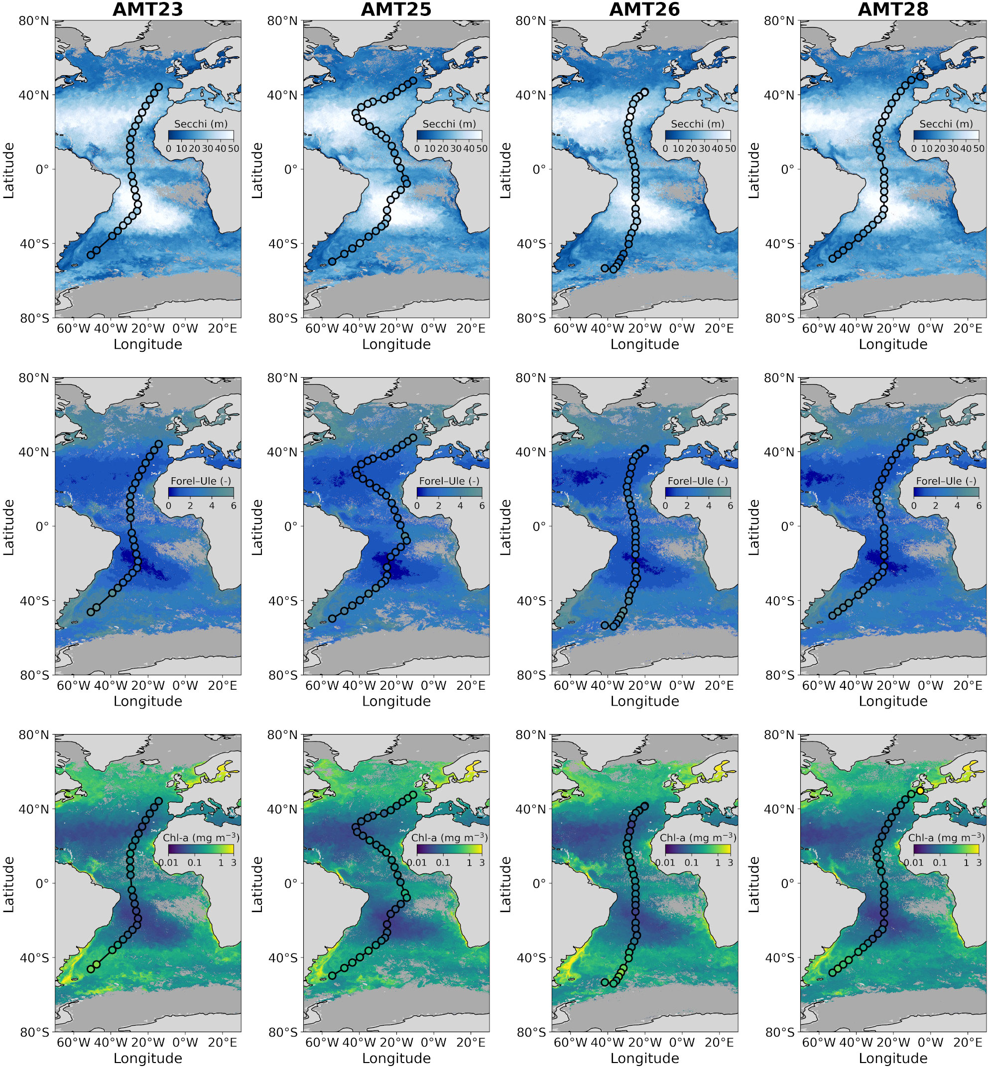
Figure 1 Locations of the 127 AMT stations where Secchi depth, Forel-Ule colour (using the LaMotte scale, for the colour of the disk at half the Secchi depth converted to infinite colour using the method of Pitarch (2017)) and Chl-a data were collected, on the four AMT cruises. The transects are overlain onto satellite estimates of Secchi depth (Pitarch et al., 2021), Forel-Ule colour (Pitarch et al., 2021), and Chl-a concentration (Sathyendranath et al., 2019), for the month of October (during which the AMT cruises took place), for each of the respective years that the cruises took place (AMT23 October 2013, AMT25 October 2015, AMT26 October 2016, AMT28 October 2018). Satellite data are from version 4.2 of the Ocean Colour Climate Change Initiative (Sathyendranath et al., 2019). The stations are coloured using the in-situ data, using the same colour scale as the satellite data, to illustrate how the two independent estimates of Secchi depth, Forel-Ule colour and Chl-a compare visually.

FIGURE 2

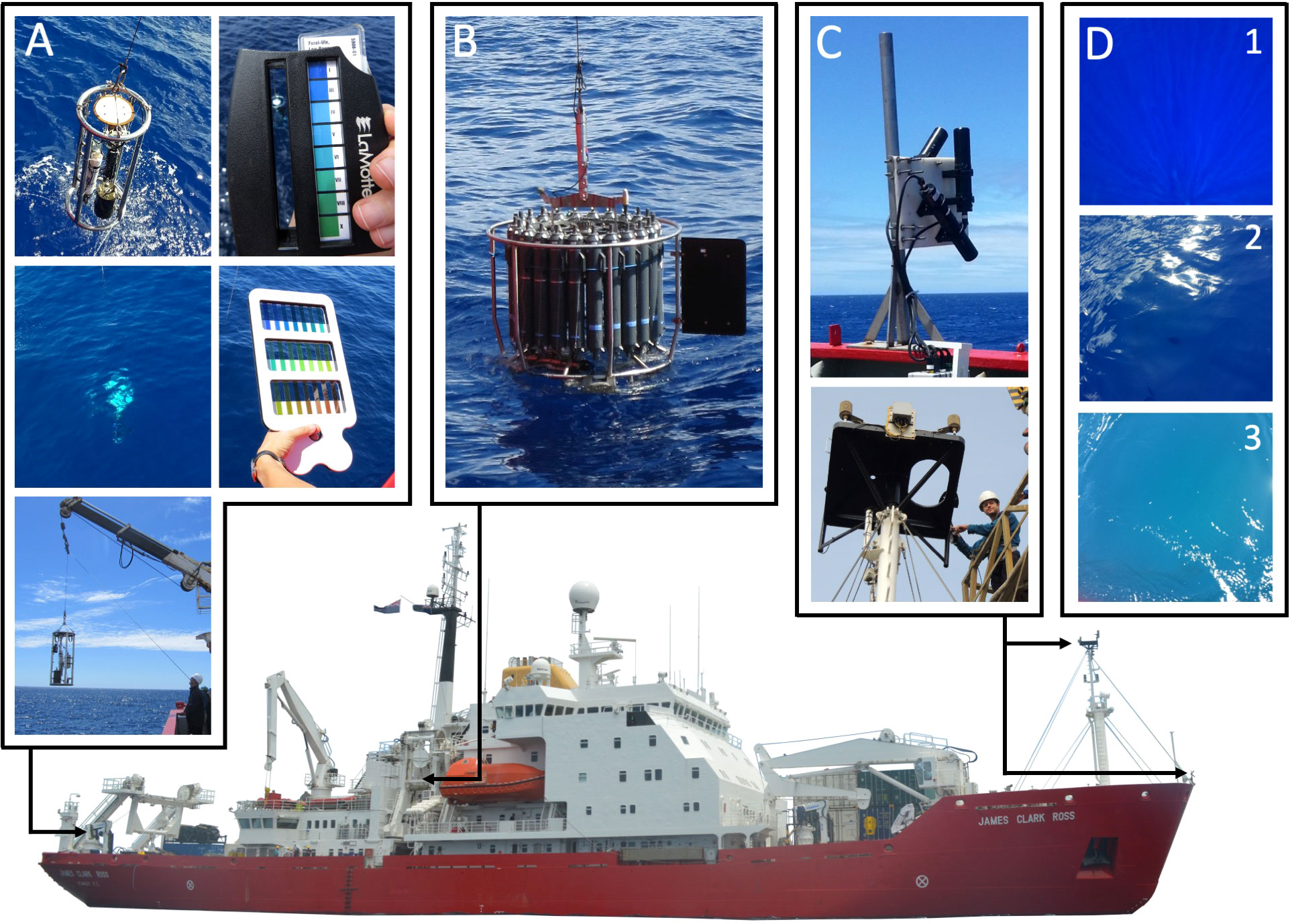
Figure 2 Instrumentation used on-board the RRS James Clark Ross. (A) Secchi disk attached to the optics rig and deployed from the aft-deck winch, with the Forel-Ule colour scales, the LaMotte scale used on AMT23-28, and that described in Novoa et al. (2014) and used on AMT25-28. (B) Conductivity, Temperature and Depth (CTD) Niskin Rossette used to collect water samples of Chl-a, measure PAR and beam attenuation, deployed on the CTD winch located towards the centre of the ship. (C) Satlantic Hyperspectral (HyperSAS) radiometer set-up (photos from AMT23), with the two radiance sensors positioned on the very bow of the ship (and tilt and heading sensor is shown vertically), and the downwelling irradiance sensor positioned vertically on the met-platform on the ship’s foremast (bottom figure showing it being attached on AMT23). (D) Photos of water colour collected on AMT23, in (1) the centre of the South Atlantic gyre, (2) the edge of the North Atlantic gyre, and (3) in the South Subtropical Convergence Zone, illustrating visual transitions from blue to blue-green waters.

2.3 Datasets collected

Table 1 lists all datasets collected and used in the study, providing acronyms, units and number of stations sampled.

TABLE 1

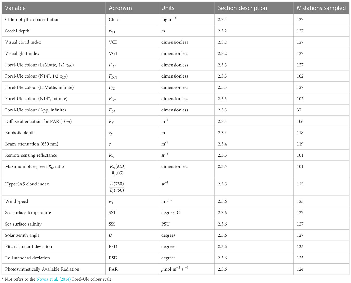
Table 1 A summary of the datasets collected and used in the study.

2.3.1 Chlorophyll-a concentration

Surface seawater samples (2-5 m depth) were collected from the CTD casts (Figure 2B, 117 stations) and from the ship underway system (six stations, where CTD casts were unavailable). Seawater was sampled into 9.5 L polypropylene carboys covered in black plastic to protect from light. Seawater samples were well mixed to avoid issues with sedimentation. Between 1-4 L samples (depending on phytoplankton biomass, e.g. 1 L in productive waters and 4 L in oligotrophic waters) were measured using the rinsed measuring cylinders, and then decanted into rinsed polypropylene bottles with siphon tubes and inverted into a six port vacuum filtration rig. Using forceps, Whatman glass fibre filters (pore size of 0.7 μm) were placed on the filter rig with the smoother side facing down. Filter papers were covered over sintered glass circles such that there were no gaps and water could only pass through the filters. Samples were filtered using a low-medium vacuum setting on the vacuum pump. When the last of the water passed through the filter paper, taps on the vacuum pump were closed and the sample filters were folded into 2 mL cryovials and either flash frozen in liquid nitrogen and transferred to the −80°C freezer (on AMT23, AMT26 and AMT28), or transferred directly to the −80°C freezer, for cases where liquid nitrogen was unavailable (AMT25).

Following each AMT campaign, High Performance Liquid Chromatography (HPLC) was used to determine total Chl-a (estimated from the sum of monovinyl chlorophyll-a, divinyl chlorophyll-a, and chlorophyllide-a). Details of the HPLC protocols and pigment extraction methods used on AMT23 and AMT25 are provided in Brotas et al. (2022), and those used on AMT26 and AMT28 are provided in Tilstone et al. (2021). At stations where neither CTD casts or underway samples were collected (four stations, one on AMT25, three on AMT26), Chl-a was estimated from underway spectrophotometric measurements of particulate absorption collected at the stations using the line-height method as described in Dall’Olmo et al. (2012), a technique proven to provide very accurate estimates of Chl-a on AMT cruises (see Dall’Olmo et al., 2012; Brewin et al., 2016; Rasse et al., 2017; Tilstone et al., 2021).

2.3.2 Secchi depth

For all four AMT cruises, a 30 cm Secchi disk was attached to the profiling rig that was deployed from the aft-deck winch of the RRS James Clark Ross (Figure 2A). Attaching the disk to the profiling rig minimised drift in all but extreme circumstances (e.g. very strong currents at the equator). The profiling rig was lowered from the surface down to around 250 m depth, and brought up from this depth to the surface, at a constant speed (that sometimes varied between down and up casts). In all but a few cases (where only one up and down cast was conducted), the profiling rig was deployed twice (two casts), and consequently, the depth of the disappearance and reappearance of the disk were measured twice (four measurements of Secchi depth at each station).

Over the four AMT cruises, the Secchi depth was measured using three different techniques. When available (principally on AMT26 and 28), a Wire Length Measurement sensor (WLM) was attached to the aft-deck winch that calculated the length of wire released by the winch. This was zeroed when the disk was at the surface, and when the disk disappeared and reappeared the observer shouted out to the winch operator who shouted back the depth, which was logged. For cases where the WLM was not available (principally on AMT23 and AMT25), the Secchi depth was measured using two alternative techniques. Firstly, and considering the profiling rig was lowered and retrieved at a set speed, the observer logged the time when the disk was at the surface, when it disappeared (or reappeared), and when the 50 m, 100 m and 150 m tags on the wire were at the surface, and did a linear interpolation to get the Secchi depth. Secondly, a watch was calibrated to the same time on a pressure sensor (CTD) on the profiling rig, and the Secchi depths were extracted by matching the time of disappearance and reappearance, with the depth from pressure sensor, correcting for distance between pressure sensor and disk. Both methods were found to agree well with a mean difference of 0.48 m (Figure 3A).

FIGURE 3

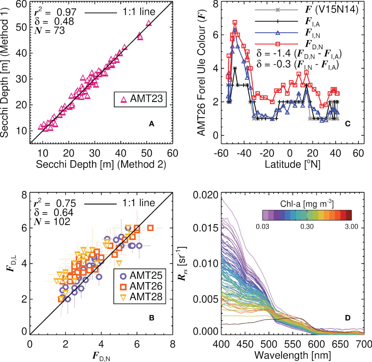
Figure 3 (A)Comparison between two methods for measuring the Secchi depth on AMT23. Method 1 involved linear interpolation, logging the time when the disk was at the surface, when it disappeared (or reappeared), and when the 50 m, 100 m and 150 m tags on wire were at the surface. Method 2 involved using a watch which was calibrated to the same time of a pressure sensor (CTD) on the profiling rig, and logging the time of disappearance and reappearance (see Section 4.3.2 for further details). Note that data are shown for all the reappearances and disappearances logged (hence there are more samples (N) than stations on AMT23). (B) Comparison between the Forel-Ule colour (F) using the method of Novoa et al. (2014) (F_D,N) and the LaMotte method (F_D,L), for the colour of the disk at half the Secchi depth on AMT25, AMT26 and AMT28. (C) AMT26 latitudinal transects of F using the method of Novoa et al. (2014), for the colour of the disk at half the Secchi depth (F_D,N), for the colour of the disk at half the Secchi depth but converted to infinite colour using the method of Pitarch (2017) (F_I,N), the Forel-Ule colour of infinite water measured using the EyeOnWater-Colour mobile phone app (Busch et al., 2016) (F_I,A), and estimated F from R_rs using the methods of van der Woerd and Wernand (2015) and Novoa et al. (2014) (V15N14). (D) Remote sensing reflectance data used in the study (101 stations) plotted as a function of wavelength and coloured according to the Chl-a concentration at the station. r² is the squared Pearson correlation coefficient, δ the mean difference (bias) and N the number of samples.

At each station, all Secchi depth data collected were averaged (denoted z_SD) and a standard deviation computed as a proxy of the uncertainty in the Secchi depth (average was 2.7 m, with an average percent deviation (standard deviation divided by z_SD) of 10%). Where possible, different participants (scientists and crew) contributed to data collection (see acknowledgements to this paper) so as to include variability between individuals. When measuring the Secchi depth, and for clear sky conditions, the measurement was often conducted on the sunny side of the ship, as there was a preference to deploy the profiling rig on the sunny side (for the Photosynthetically Available Radiation (PAR) sensor on the main CTD). At low latitudes in the tropics (especially near the equator), the sun zenith angle was very low at the noon stations (sun high in the sky), making it difficult to avoid the sun (i.e. both sides of the ship were sunny). The observer often took notes of the conditions, that were subsequently used to indicate if the sky was fully overcast or clear/partial cloud (when reported, denoted VCI), and when sun glint was reported as a problem when collecting data (denoted VGI).

2.3.3 Forel-Ule colour

Two different Forel-Ule (F) scales were used in the study (shown in Figure 2A). A LaMotte scale was used on all four AMT cruises, which consists of a simple printed scale encased in perspex, showing F colours 1, 3, 4, 5, 6, 7, 8, and 9 (missing 2). Additionally, on AMT25, AMT26 and AMT28, the Forel-Ule scale presented in Novoa et al. (2014), and kindly provided by Marcel Wernand, was also used (with all F numbers). At the majority of stations, four F measurements were collected, for the two up and down casts (at stations where only one cast was made, two measurements were collected). The measurements were collected by comparing the colour of the disk at roughly half the Secchi depth (approximated based on a priori knowledge). As with the Secchi depth, many participants (scientists and crew) contributed to Forel-Ule data collection (see acknowledgements to this paper), many at the same time using the different scales, so as to include variability between individuals. At each station, and separately for each scale, all measurements collected were averaged and a standard deviation computed as a proxy of the uncertainty. Comparisons between the colour of the disk using the LaMotte scale (F_D,L) and the colour of the disk using the Novoa et al. (2014) scale (F_D,N) are shown in Figure 3B, and are in reasonable agreement (r² = 0.75), but with the LaMotte scale generally higher than the Novoa et al. (2014) scale (δ = 0.64). These measurements were also converted from the colour of the water above the disk at half the Secchi depth, to the colour of infinite water (F_I,L and F_I,N, where I refers to the conversion to infinite colour), using the algorithm of Pitarch (2017) and a lower boundary of F = 0 (Pitarch et al., 2019). This method consists of converting F to hue angle, applying a polynomial relationship to convert the hue angle of the water above the disk at half the Secchi depth to the hue angle of infinite water, then converting back to F (Pitarch, 2017). For stations on AMT26, the F colour was also measured using the EyeOnWater-Colour mobile phone app (www.eyeonwater.org; Novoa et al., 2015; Busch et al., 2016; Malthus et al., 2020), for infinite water (not using the disk, denoted F_I,A), which gave a single number for each station. The measurement was collected in a direction away from sun glint (typically between 100-170 degrees azimuth). Comparisons between F_I,A and F_I,N on AMT26 are shown in Figure 3C. The F_I,N data are in good agreement with F_I,A, with a mean difference of −0.3 compared with −1.4 for the unconverted data (F_D,N), supporting the conversion method.

2.3.4 Diffuse and beam attenuation

On all four AMT cruises, a WET Labs C-Star, designed to measure beam attenuation (c) at 650 nm, was attached to the base of the main CTD, and a Biospherical QCD-905L sensor, designed to measure downwelling PAR, was attached to the top of the CTD (Figure 2B). Both sensors provided vertical profiles of c and PAR, for stations where the main CTD was deployed. Data for downcasts were extracted from the CTD logger, which was preferred over upcast data when bottles were fired (CTD stopped to shut the Niskin bottles at discrete depths on the upcast).

Data for c were processed as follows: firstly, a cruise specific minimum value of c derived from all profiles used for each cruise, were subtracted from the profile, this minimum value (which varied among cruises) represented that of pure water beam attenuation [c_w(650)] and any residual biases in the calibration; secondly, values of c_w(650) (c_w=b_w+a_w, where a_w is the absorption coefficient of pure water, taken from Pope and Fry (1997), and b_w the scattering coefficient of pure water, which was computed as a function of sea surface temperature (SST) and salinity (SSS) at each station following Zhang and Hu (2009) and Zhang et al. (2009), see Section 4.3.6 for details on how SST and SSS were collected) were added back to the profile, which resulted in calibrated profiles of c. Data were extracted from between the surface and Secchi depth, and median values of c and standard deviations (range of distribution that lies within the percentiles of one standard deviation) were computed. Data for c were only retained if the coefficient of variation for the samples in the Secchi depth layer was less than 0.04. Considering this method assumes c_p(650) and c_y(650) are close to zero at depth (y representing coloured dissolved organic matter), which may not always hold, it is possible the c values are slightly biased low.

Vertical profiles of PAR were used to compute the diffuse attenuation coefficient of PAR (K_d). Two values of K_d were derived for each profile, K_d(10%) in the layer between the surface and the 10% light level (defined as 2.3/K_d), and K_d(1%) in the layer between the surface and the 1% light level (defined as 4.6/K_d). The latter was used to compute the euphotic depth (z_p=4.6/K_d(1%)), and the former was used to represent K_d (i.e., K_d = K_d(10%)) in the Secchi depth layer (Lee et al., 2018c). Both were computed as follows: firstly, the 10% and 1% light depth levels were approximated from the surface Chl-a concentration using an AMT-calibrated model (Brewin et al., 2017); PAR data above these depth levels were extracted and initial values of K_d for the two depth levels were derived by fitting a Beer-Lambert law (acknowledging this assumes inherent optical properties to be constant in the layer) to the PAR and depth data (using IDL function ROBUST_LINEFIT.pro, an outlier-resistant fitting function); next, these initial values were used to recompute the 10% land 1% light depth levels, and the data were re-fitted to PAR and depth data above these light depth levels, to derive final values for K_d and z_p. Standard deviations for K_d were also extracted from the fits. To remove dubious data (from unusual profiles), K_d and z_p for a given profile were only retained if the r² between log(PAR) and depth, above the respective light level, was greater than 0.85.

2.3.5 Remote sensing reflectance data and ocean colour models

The same Satlantic/Seabird Hyperspectral (HyperSAS) radiometer package was installed on the RRS James Clark Ross for all four AMT cruises. Sensors were calibrated prior to the start of each cruise. The hyperspectral downwelling irradiance (E_s) sensor was attached to the met-station on the ship’s foremast (Figure 2C), to minimise obstructions from the ship shading the sensor. The two radiance sensors, measuring total water leaving radiance (L_t) and sky radiance (L_i), were mounted at the identical azimuth angle, and pointed at the water surface at an angle of 40° from nadir and zenith respectively (Figure 2C). Data were collected at a frequency of 1-5 seconds, during day light hours.

Hyperspectral (at 2 nm resolution) remote sensing reflectance data (R_rs) were computed using the method described in Lin et al. (2022). Briefly, this involved: interpolating the dark counts (collected at 10-minute intervals) for each sensor, to the times of the light data, and subtracting them from the light measurements; interpolating the (dark-count-corrected) light data to a common set of wavelengths (350 to 860, at 2 nm resolution) and a common time (based on the sensor with the slowest integration time); interpolating auxiliary ship data (wind, latitude, longitude, time, wind, heading, tilt, pitch, and roll) used for data filtering to the same time as the light measurements; filtering data according to a set criteria (<5° tilt, removing sun glint using the near-infrared signal, discarding data with high solar zenith angle (>80°) and relative azimuth angles <100 and >170°, and any spectra with negative values at 443 nm); and computing R_rs by first computing water leaving radiance according to L_w=L_t−ρL_i−ΔL, where ρ is the sea-surface reflectance used to correct for the sun and sky light reflected by the sea surface, and ΔL is a spectrally-flat residual term representing contributions due to glint, foam, sea spray and whitecaps (both derived using an non-linear optimization technique), then dividing L_w by E_s to get R_rs. Further details of the processing are provided in Lin et al. (2022). In addition to R_rs, the method of Lin et al. (2022) also included a full uncertainty propagation method, following the Law of Propagation of Uncertainty, and provides robust uncertainty estimates with each R_rs measurement (see Lin et al. (2022) for further details).

At each station for which R_rs data passed the filtering criteria, data were extracted between 20 minutes prior to and 60 minutes after the start time of the station (stations were typically >1 hour in duration). Data 20 minutes prior were included, as at this point, the ship slows down to arrive at the station and reorientates its position, allowing data to be available (during the orientation process) for cases where the ship’s final position (relative azimuth angle) at the station was not ideal for data collection. All 2-min binned R_rs data available during this period at each station were analysed and the spectra with the lowest average R_rs uncertainty between 400-600 nm were selected (data outside the range of 0 and 20% uncertainty were excluded). This resulted in R_rs data at 101 stations. R_rs data were bidirectionally corrected using the method of Lee et al. (2011) and are plotted in Figure 3D and coloured according to the Chl-a concentration at the station. A proxy of sky conditions was also derived using the ratio of L_i(750)/E_s(750), using data processed over a one hour duration after the start of the station following the method of Brewin et al. (2016), removing any unrealistic data where the ratio was $\ge 1/\pi$. Median values of L_i(750)/E_s(750) were extracted from each station as were standard deviations (defined as the range of distribution that lies within the percentiles of one standard deviation). Clear skies are known to be approximately 0.02 (Mobley, 1999) and fully overcast in the order 0.3 (Ruddick et al., 2006). To cross-check with the notes from the Secchi disk observations, we computed the median of all L_i(750)/E_s(750) data where the observer had reported overcast skies and found that to be 0.264 ( ± 0.083) and the median of all other stations to be 0.046 ( ± 0.068), showing consistency in the two datasets.

The in-situ R_rs data were used to compute the maximum blue-green band ratio (max{R_rs(443), R_rs(490), R_rs(510)}/R_rs(555)), hereafter denoted R_rs(MB)/R_rs(G) that was subsequently used to show changes in the relationship between the maximum band ratio and Chl-a concentration, using the NASA OC4v6 algorithm (NASA, 2010). Additionally, Secchi depth (z_SD) was estimated from R_rs and the solar zenith angle (see Section 2.3.6) data using the algorithms of Lee et al. (2015) and Jiang et al. (2019). An initial step in the computation of z_SD using both algorithms, is the estimation of inherent optical properties from R_rs, using the Quasi-Analytical Algorithm (QAA) (Lee et al., 2002, 2009). Here, we incorporated a Raman scattering correction on R_rs prior to inversion, following Pitarch et al. (2020), and used updates on the parameters that relate non-water absorption at 555 nm to R_rs, as described in Pitarch and Vanhellemont (2021). The Forel-Ule colour (F) was estimated from hyperspectral R_rs data by computing the hue angle using the approach of van der Woerd and Wernand (2015) and then converting the hue angle into F following Novoa et al. (2014).

2.3.6 Auxiliary observations

A series of auxiliary measurements were averaged (mean of 90 percentile distribution) over the duration of each station (1 h after the start time of the station), and standard deviations computed (range of distribution that lies within the percentiles of one standard deviation). These data include: wind speed (w_s) measurements, which were collected continuously from the anemometer located on the met-platform of the ship’s foremast (Figure 2C), and corrected for ship direction, course and speed (following https://www.coaps.fsu.edu/woce/truewind/true-IDL.html); SST and SSS, when not available from the main CTD (taken as the median temperature and salinity values in layer between surface and z_SD), were extracted from continuous measurements collected by the ships underway CTD (SBE45); solar zenith angles (θ) were computed as a function of time and location of the stations; standard deviations in the pitch (PSD) and roll (RSD) of the ship were taken from continuous measurements collected by the ship’s gyro system; and above-surface PAR data were collected from the PAR sensor (Kipp & Zonen) located on the met-platform of the ship’s foremast.

In addition to AMT observations, we also used two databases of Secchi depth and Forel-Ule colour measurements, collected globally since 1890, from the US National Oceanographic Data Center (NODC) and from CalCOFI. NODC data were taken from the dataset assembled by Boyce et al. (2012) and are designed to represent global, case-1 (open ocean) conditions. Boyce et al. (2012) describe the NODC data mining and processing. Briefly, nearshore, shallow and unrealistic data were eliminated, and remaining data binned into one-by-one degree geographical cells. High sediment and CDOM-laden measurements were removed by eliminating Secchi disk depth measurements less than 6 m. Forel-Ule measurements were constrained to values between 2 and 10. The total amount of NODC Secchi disk and Forel-Ule data used was 46,180 data points. The data are available through the NODC website (https://www.ncei.noaa.gov/data/oceans/woa/WOD/DATA_SUBSETS/). The CalCOFI site is in clear waters off the Californian coastline, and has been operating since 1949. Sampling was made following a defined grid geographically distributed between 20°N and 40°N, and measurements were collected at a relatively consistent rate across the seasons. Data are downloadable from the project site (https://calcofi.org/). Matched Secchi disk and Forel-Ule data exists between 1969 and 1972 and then from 1986 to 1998, and amounts to a total of 2046 matched data points.

3 Results and discussion

3.1 Comparison of optical measurements on AMT

Figure 4 shows a comparison of optical measurements collected on the four AMT cruises. Consistent with previous understanding (e.g., Wernand, 2011), we see tight inverse relationships between Secchi depth (z_SD) and Forel-Ule colour (F), with F explaining between 73-83% of the variance in z_SD, depending on the colour scale used (see Figures 4A–D). For the colour of the disk (at 1/2 the Secchi depth, F_D,L and F_D,N), and over the range of data collected, there appears to be a log-linear relationship between variables (Figures 4A, B). For infinite depth, the LaMotte scale (F_D,L) also show a log-linear relationship (Figure 4C), but the Novoa et al. (2014) scale (F_I,N) is closer to a log-log relationship, consistent with earlier models (Wernand, 2011, see Figure 4D), albeit with differences in parameters. Figure 5 overlays the AMT data collected using the Novoa et al. (2014) scale onto historical datasets from NODC and CalCOFI. We find the relationship between z_SD and infinite colour (F_I,N) on AMT to be in closer agreement with relationships between z_SD and F seen in both historical datasets, when compared with data on z_SD and the colour of the disk at 1/2 the Secchi depth (F_D,N). Particularly for lower F values (1-3). This result suggests that the majority of the Forel-Ule historical data may have been collected by looking directly at the colour of the water, rather than at the colour of the water above the disk at 1/2z_SD, as other literature has implied (Wernand and van der Woerd, 2010a). Further investigation is needed to ascertain if this is in fact correct, perhaps by reviewing historical information on the protocols used for collecting these earlier Forel-Ule measurements.

FIGURE 4

Figure 4 Comparison of optical measurements collected on the four AMT cruises. (A–D) Secchi depth (z_SD) versus Forel-Ule colour (F), with subscripts D being colour of disk, I colour of infinite waters, L the LaMotte scale, and N the scale of Novoa et al. (2014). (E–H) Maximum blue-green R_rs ratio (R_rs(MB)/R_rs(G)) versus Forel-Ule colour (F). (I) Secchi depth (z_SD) versus R_rs(MB)/R_rs(G). (J) Diffuse attenuation for PAR (10% light level, K_d) versus Secchi depth (z_SD). (K) Beam attenuation (650 nm) (c) minus that of pure water (c_W) versus Secchi depth (z_SD). (L) Euphotic depth (z_p) versus Secchi depth (z_SD). Solid lines are models fitted to the data. Dashed lines are earlier models, with W11 referring to the model of Wernand (2011) and L18 referring to models from Lee et al. (2018c).

FIGURE 5

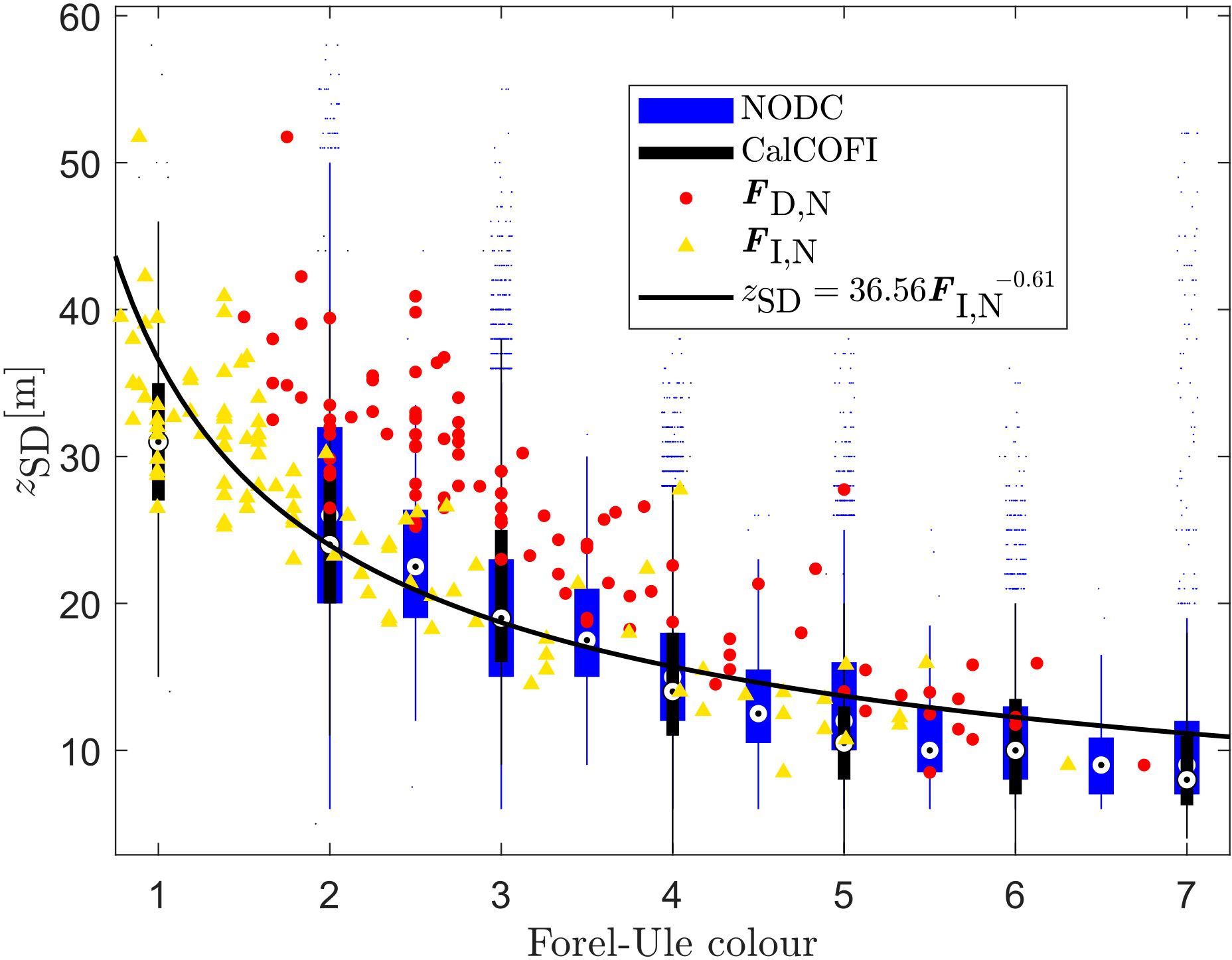
Figure 5 Comparison of Secchi depth (z_SD) versus Forel-Ule colour (F) data collected on AMT (red circles and yellow triangles) with historical datasets from NODC and CalCOFI. Note that F_I,N is a synthetic quantity that derives from F_D,N and the model in Pitarch (2017).

On AMT, relationships between the maximum band ratio (R_rs(MB)/R_rs(G)) and F (Figures 4E–H) are remarkably consistent with the relationships seen between z_SD and F (Figures 4A–D), with F explaining between 69-80% of the variance in R_rs(MB)/R_rs(G). This is due to a tight relationship observed between z_SD and R_rs(MB)/R_rs(G) (Figure 4I). Inverse relationships between both diffuse and beam attenuation and z_SD were also observed (Figures 4J, K), with the former (K_d=1.3/z_SD) in good agreement with the relationship proposed by Lee et al. (2018c), (Figure 4J, K_d = 1.48/z_SD), with differences possibly related to environmental conditions, considering the Lee et al. (2018c) relationship is for a fixed solar zenith angle (θ) of 30 degrees, and a fixed wind speed (w_s) of 5 ms⁻¹. We also see good agreement between the euphotic depth (z_p) and z_SD (Figure 4L, z_p=3.67z_SD), with no significant difference to the relationship proposed by Lee et al. (2018c) (where z_p is equal to 3.55 (± 0.15) times z_SD).

3.2 Relationships between surface Chl-a and optical properties on AMT

Figure 6 shows a comparison of Chl-a and optical measurements collected on the four AMT cruises. We find z_SD to be tightly correlated with Chl-a, explaining around 85% of its variance (r²=0.85, on log₁₀-transformed variables). The relationship between z_SD and Chl-a is in good agreement with published models (Table 2; Morel et al., 2007; Boyce et al., 2012; Lee et al., 2018c). Systematic differences (accuracy, δ) are close to zero for the models of Morel et al. (2007) and Lee et al. (2018c), with the a small bias for the model of Boyce et al. (2012) (Table 2). The models of Boyce et al. (2012) and Lee et al. (2018c) have slightly better precision (Δ, Table 2) than the Morel et al. (2007) model. Fitting a power-law model to the data [Table 2, the same mathematical model to that of Lee et al. (2018c) and Boyce et al. (2012)] reduces the bias (δ) to zero, with no improvement in precision (Δ), and obtained parameters are found not to be significantly different to those of Lee et al. (2018c) (Table 2). Statistical tests indicate that the retrieval of surface Chl-a from z_SD is comparable, in precision and accuracy, to retrievals of Chl-a using satellite ocean colour algorithms in the Atlantic Ocean (Brewin et al., 2016; Tilstone et al., 2021). Residuals in log₁₀(Chl-a), between the fitted power model and Chl-a data, were positively correlated with wind speed and R_rs(MB)/R_rs(G), and inversely correlated with log₁₀(Chl-a) (Table 3). The latter two (which are inversely related, see Figure 6B) perhaps suggesting the mathematical formulation of the relationship (power function) may need further consideration, with there being a slight tendency for the model to overestimate log₁₀(Chl-a) at lower concentrations and underestimate it at higher concentrations. Other fitting functions were explored, including log-linear and polynomial fits (data not shown), but they also showed the same tendency, suggesting this may be related to the distribution of the dataset. The positive correlation between residuals and wind speed (Table 3), suggested that for the same Chl-a, as the wind speed increases, the observer sees a shallower Secchi depth. This is consistent with theory on the impact of wind speed on the apparent contrast of the disk (Preisendorfer, 1986). However, multi-linear regression (not shown) of log₁₀(Chl-a) as a function of both log₁₀(z_SD) and wind speed, yielded no significant increase in r² over log₁₀(z_SD) alone (Z-test, p>0.05), suggesting any such effect is minor. No relationship was found between the VGI and VCI, and the residuals in log₁₀(Chl-a), between the fitted power model and Chl-a data.

FIGURE 6

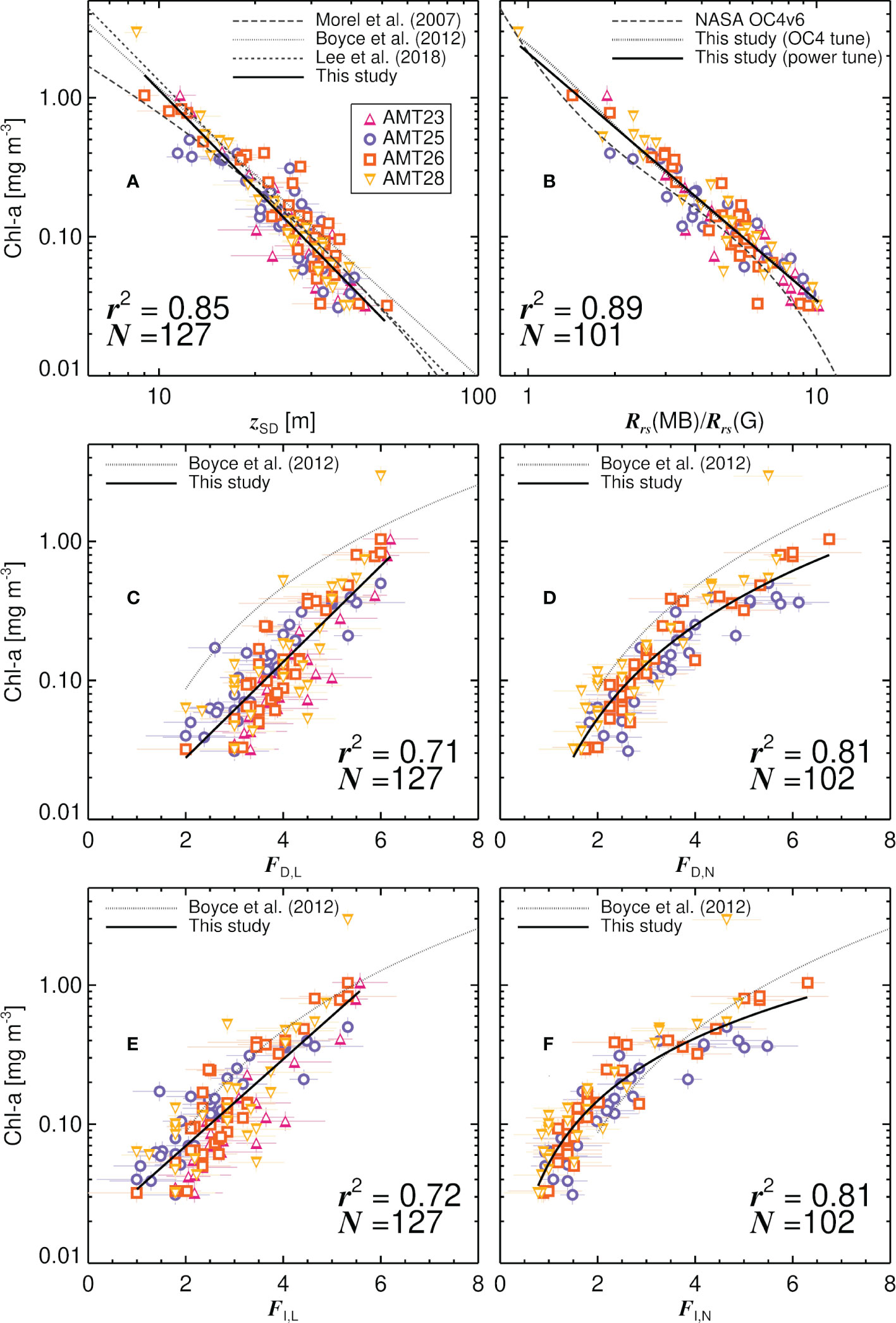
Figure 6 Relationship between historical and modern optical properties and the chlorophyll-a concentration (Chl-a) on the four AMT cruises. (A) Comparison of Chl-a and Secchi depth (z_SD). (B) Comparison of Chl-a and maximum blue-green R_rs ratio (R_rs(MB)/R_rs(G)). (C) Comparison of Chl-a and Forel-Ule colour using the LaMotte scale and with reference to the colour of the disk at 1/2z_SD (F_D,L). (D) Comparison of Chl-a and Forel-Ule colour using the Novoa et al. (2014) scale and with reference to the colour of the disk at 1/2z_SD (F_D,N). (E) Comparison of Chl-a and Forel-Ule colour using the LaMotte scale and with reference to infinite water (F_I,L). (F) Comparison of Chl-a and Forel-Ule colour using the Novoa et al. (2014) scale and with reference to infinite water (F_I,N).

TABLE 2

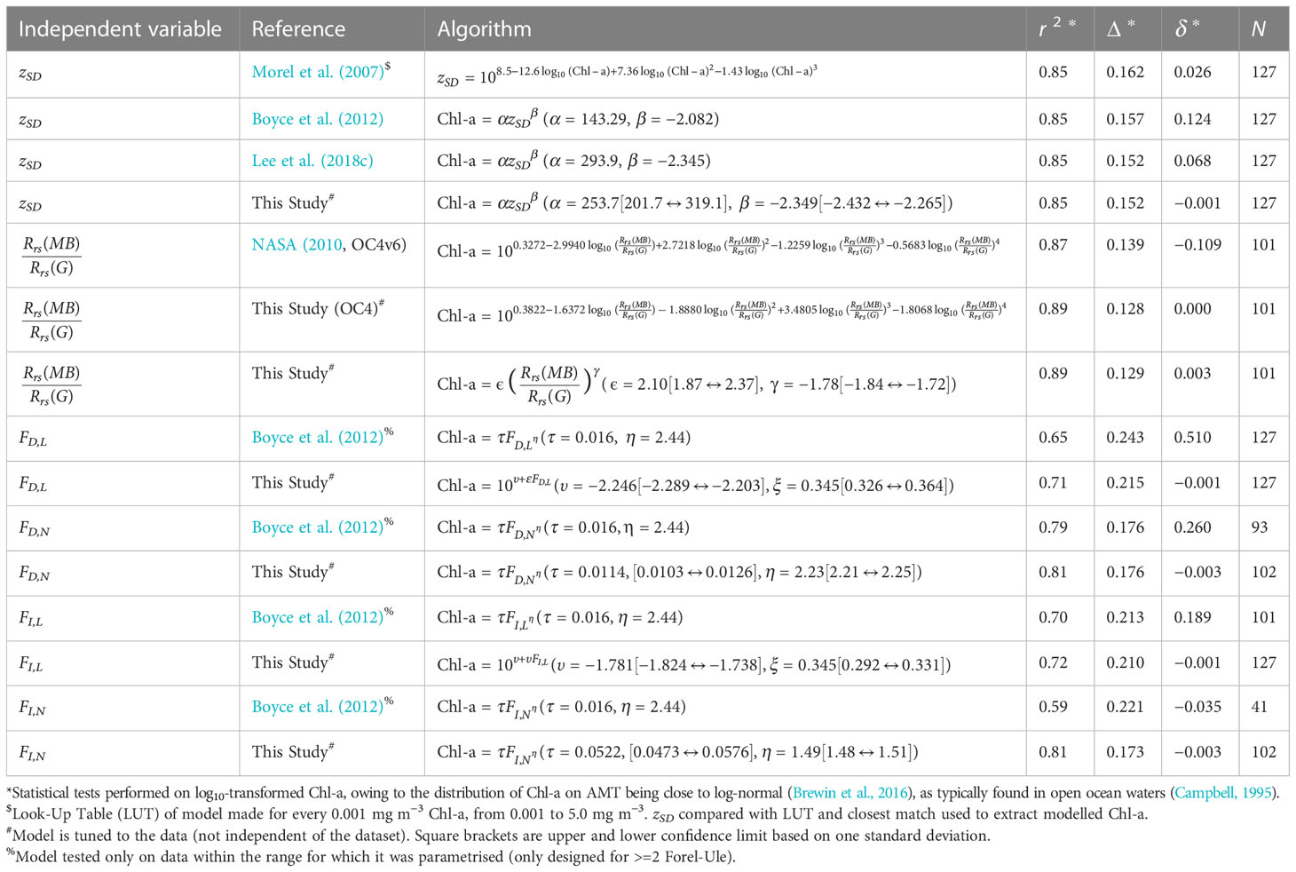
Table 2 Algorithms tested to predict Chl-a [mg m⁻³] (dependent variable) from historic and modern optical measurements (independent variable, models tuned to data, denoted “This Study” in Table 2).

TABLE 3

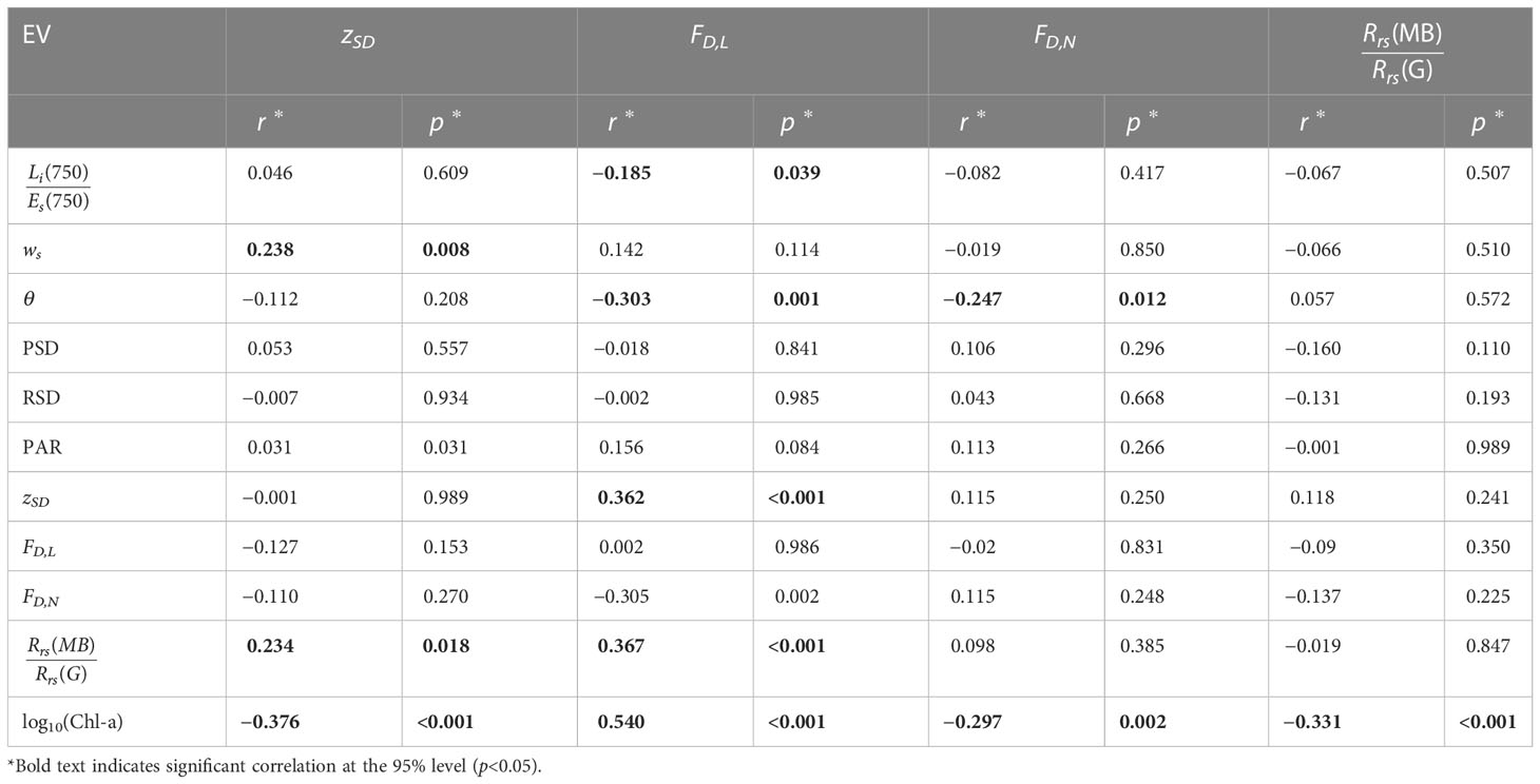
Table 3 Residuals between estimated log₁₀(Chl-a), from Z_SD, F_D,L, F_D,N and R_rs(MB)/R_rs(G) (independent variables), and measured log₁₀(Chl-a), correlated with environmental variables (EV).

Of all the optical proxies tested, R_rs(MB)/R_rs(G) was found to explain the greatest variance in Chl-a (Figure 6B, r²= 0.89, on log₁₀-transformed variables). The NASA OC4v6 algorithm was found to have a tendency to underestimate Chl-a in the Atlantic (Table 2, δ = −0.109), consistent with earlier work (Szeto et al., 2011). A retuning of the OC4v6 algorithm removed this bias, and showed improvements in both precision (Δ) and r² (Table 2). The retuning was also found to show a strong linear dependency (on log₁₀-transformed data) between variables, suggesting a simpler (more parsimonious) linear model to be more appropriate than a 4th order polynomial on this AMT dataset, which yielded statistically similar results to the retuned polynomial (OC4 Table 2). We found a small dependency in the residuals of this linear model and log₁₀(Chl-a), similar to the z_SD fits and likely related to data distribution, but no other dependency between residuals and other environmental variables were observed (Table 3). R_rs(MB)/R_rs(G) was shown to produce the highest r² and lowest Δ of all variables tested (Table 2). R _rs(MB)/R_rs(G) only performs marginally better as a predictive variable of Chl-a, than z_SD (Table 2), on the AMT.

All four Forel-Ule datasets (F_D,L, F_D,N, F_I,L and F_I,N) were positively correlated with Chl-a, explaining between 71-81% of the variance in log₁₀-transformed Chl-a (Figures 6C–F). The Novoa et al. (2014) scale data (F_D,N, F_I,N) were found to correlate more tightly to Chl-a (explaining around 81% of the variance) than the LaMotte scale data (explaining around 71% of the variance), with the Novoa et al. (2014) scale data predicting Chl-a with the highest accuracy using a power function (linear-function in log₁₀ space), consistent with the model of Boyce et al. (2012), with the LaMotte scale data best described using a log-linear relationship (Figures 6C–F; Table 2). For Forel-Ule data greater than 2, the lower limit of the range of data in which the Boyce et al. (2012) model was trained on, the Boyce et al. (2012) model is seen to overestimate Chl-a when using F_D,L and F_D,N as input (Figures 6C, D; Table 2), with better agreement (biases (δ) closer to zero) when using F_I,L and F_I,N as input (Figures 6E, F; Table 2). This is consistent with the Forel-Ule infinite colour data collected on AMT being in closer agreement with historical datasets than data collected on the colour of the water above the disk at 1/2z_SD (Figure 5), considering the Boyce et al. (2012) model was parameterised on these historical data. As with the z_SD and R_rs(MB)/R_rs(G) models, there is a dependency in Forel-Ule model residuals (log₁₀(Chl-a) model minus data) on log₁₀(Chl-a) (Table 3, positive for F_D,L and negative for F_D,N), likely related to data distribution. The LaMotte model residuals were also correlated with L_i(750)/E_s(750), R_rs(MB)/R_rs(G) and z_SD (Table 3). Residuals in both models were also found to be correlated with solar zenith angle (Table 3). This may suggest the sky conditions had some impact on data collection, possibly influencing the apparent colour of the disk, although no relationship was found between residuals and the VGI and VCI. Whereas measuring Forel-Ule of infinite water directly is useful for testing the Pitarch (2017) conversion, and more in-line with the historical observations (Figure 5), it is difficult to observe subtle variations in Chl-a at low concentrations, since the Forel-Ule saturates at the lowest value (Figure 3C). In fact, this is a key reason Boyce et al. (2012) excluded Forel-Ule data less than two in their algorithm. Instead, by measuring the colour of the disk at 1/2z_SD, the observer can track these subtle changes in colour at very low Chl-a (Figure 6), as the scale has not saturated at its lowest value.

Whereas it is clear from this analysis that modern optical tools for estimating Chl-a (R_rs(MB)/R_rs(G)) performed the best (Table 2), it is nonetheless remarkable how well the historical tools performed, with some (e.g., z_SD) only marginally lower in performance than the modern method, and with a higher number of observations (less effected by environmental constrains in data collection). These results supports the merging of historical data with modern methods (e.g., satellite remote sensing) in search of long term trends in Chl-a, providing systematic differences can be identified, and acknowledging the challenges in bridging data collected at very different temporal and spatial scales (Boyce et al., 2010; Rykaczewski and Dunne, 2011; Boyce et al., 2012; Boyce et al., 2014). Models proposed here are nonetheless limited to the range of data they have been calibrated with, to case-1 open-ocean waters, and to the Atlantic Ocean. Caution is also needed when applying such models, developed between 2013-2018, to data collected in the past, since the relationships among Secchi depth, Forel-Ule colour, R_rs, and Chl-a, could themselves be sensitive to climate change.

3.3 Evaluating algorithms for estimating Secchi depth and Forel-Ule colour from remote-sensing reflectance on AMT

The AMT is, and has been, widely used as a platform for evaluating Chl-a remote-sensing algorithms (O’Reilly et al., 1998; Brewin et al., 2016; Tilstone et al., 2021), owing to the fact the transect samples such a wide variety of biogeochemical provinces. Here, we extend the range of remote-sensing variables evaluated on AMT, to include the Secchi depth and Forel-Ule colour.

Figure 7A and Table 4 show results from a statistical comparison between Forel-Ule data derived using the R_rs-based methods of van der Woerd and Wernand (2015) and Novoa et al. (2014) and that from the four in-situ datasets collected on AMT. The R_rs-based method performs well in the comparison, with r² values ranging from 0.64 to 0.70, and unbiased root mean square differences (Δ) ranging from 0.48 to 0.71 (Table 4). As expected, the R_rs-based method is in better agreement with the infinite colour in-situ datasets, with biases (δ) closer to zero for F_I,L, F_I,N and F_I,A, than for F_D,_L, F_D,N (Table 4). Linear regression between data shows the biases to vary systematically over the range of Forel-Ule data, with the F_I,L and F_I,N in better agreement with the R_rs-based method at lower values (<4), but deviating significantly at higher values (>4, Figure 7A; Table 4), with differences (residuals) between the R_rs-based method and F_I,N data inversely correlated with changes in Forel-Ule (Table 5). These residuals were also found to be correlated with wind speed, the pitch and roll of the vessel, the Secchi depth and log₁₀(Chl-a) (Table 5). Interestingly, the slope of the regression in the statistical comparison between the R_rs-based method and F_I,A (phone app) data was closer to one, and the bias (δ) closer to zero, when compared with other data (Table 4). Furthermore, differences (residuals) between the R_rs-based method and F_I,A data were not significantly correlated with any environmental variables (data not shown), acknowledging that only one cruise (AMT26) of F_I,A data were available in the analysis. Figure 3C shows the transect of F data for AMT26. All infinite F data are in good agreement at low values, but at higher values towards the end of the cruise (in the South Atlantic), the F_I,L and F_I,N are significantly higher than both the F_I,A (phone app) data and the R_rs-based method, with the latter two in very good agreement. It may be that the conversion between the colour of the disk and infinite colour used here (Pitarch, 2017) to derive F_I,L and F_I,N, which performs very well at lower values (<4) (Figure 3C), requires revaluation at higher F values (>4).

FIGURE 7

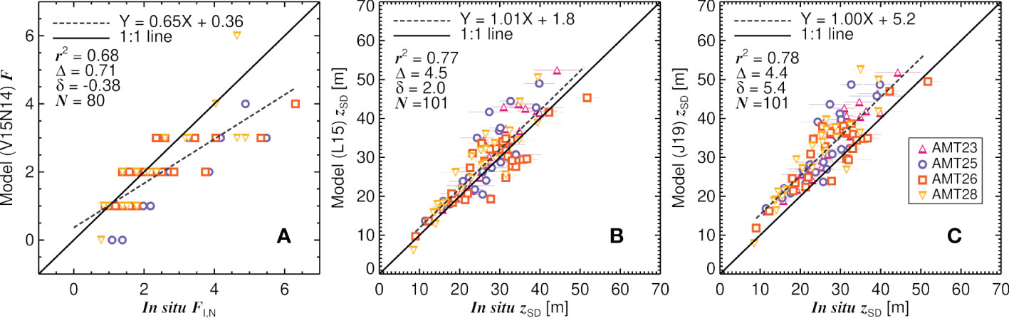
Figure 7 Comparison of R_rs-derived Forel-Ule colour (F) and Secchi depth (z_SD) with in-situ data. (A) R_rs-derived F using the methods of van der Woerd and Wernand (2015) and Novoa et al. (2014) (V15N14) with in-situ F_I,N (F measured using the scale of Novoa et al. (2014) for the colour of the disk at half the Secchi depth, but converted to infinite colour using the method of Pitarch (2017)). (B) R_rs-derived z_SD using the model of Lee et al. (2015) (L15) against in-situz_SD. (C) R_rs-derived z_SD using the model of Jiang et al. (2019) (J19) against in-situ z_SD. r² is the squared Pearson correlation coefficient, δ the mean difference (bias), Δ the unbiased root mean square difference, and N the number of samples.

TABLE 4

Table 4 Comparison of R_rs-derived F using the R_rs-based methods of van der Woerd and Wernand (2015) and Novoa et al. (2014) with various in-situ F datasets collected on AMT.

TABLE 5

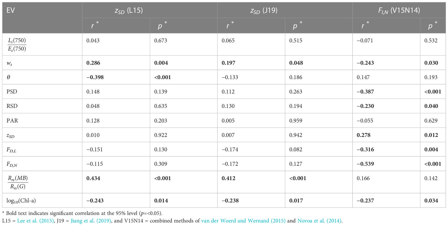
Table 5 Residuals between estimated z_SD or F using R_rs-based models and in-situ data correlated with environmental variables (EV).

A statistical comparison between in-situ z_SD and the R_rs-based algorithms of Lee et al. (2015) and Jiang et al. (2019) are shown in Figures 7B, C. Within the range of in-situ z_SD collected on the AMT cruises (8.5 - 51.8 m), both algorithms perform reasonably at retrieving z_SD from R_rs, with r² values ranging from 0.77 to 0.78, unbiased root mean square differences (Δ) ranging from 4.4 to 4.5 m, and linear regression slopes close to one. Both R_rs-based algorithms show slightly higher estimates than the in-situ z_SD data (positive biases (δ)), but biases for the Lee et al. (2015) algorithm are closer to zero (δ = 2.0) than for the Jiang et al. (2019) algorithm, where there is a systematic overestimation of z_SD of around five meters (δ = 5.4). Interestingly, there was no significant change in model performance when removing stations with overcast conditions (VCI = 1). However, it is important to recognise both models were calibrated with Hydrolight simulations using cloudless skies (Lee et al., 2002, 2005, 2009).

3.4 On the dependency of Secchi depth on solar zenith angle and wind speed

Differences (residuals) between the Lee et al. (2015) and Jiang et al. (2019) algorithms, and the in-situ z_SD data, were both found to be positively correlated with R_rs(MB)/R_rs(G) and inversely correlated with log₁₀(Chl-a) (Table 5). Residuals between the Lee et al. (2015) algorithm and the in-situ z_SD data were inversely correlated with solar zenith angle (θ), but not in the case of the Jiang et al. (2019) algorithm (Table 5 and Figure 8). Both algorithms incorporate a dependency on θ in the conversion of IOPs [derived analytically from R_rs following Lee et al. (2002, 2005, 2009)] to K_d(λ), and both algorithms subsequently derive z_SD according to

FIGURE 8

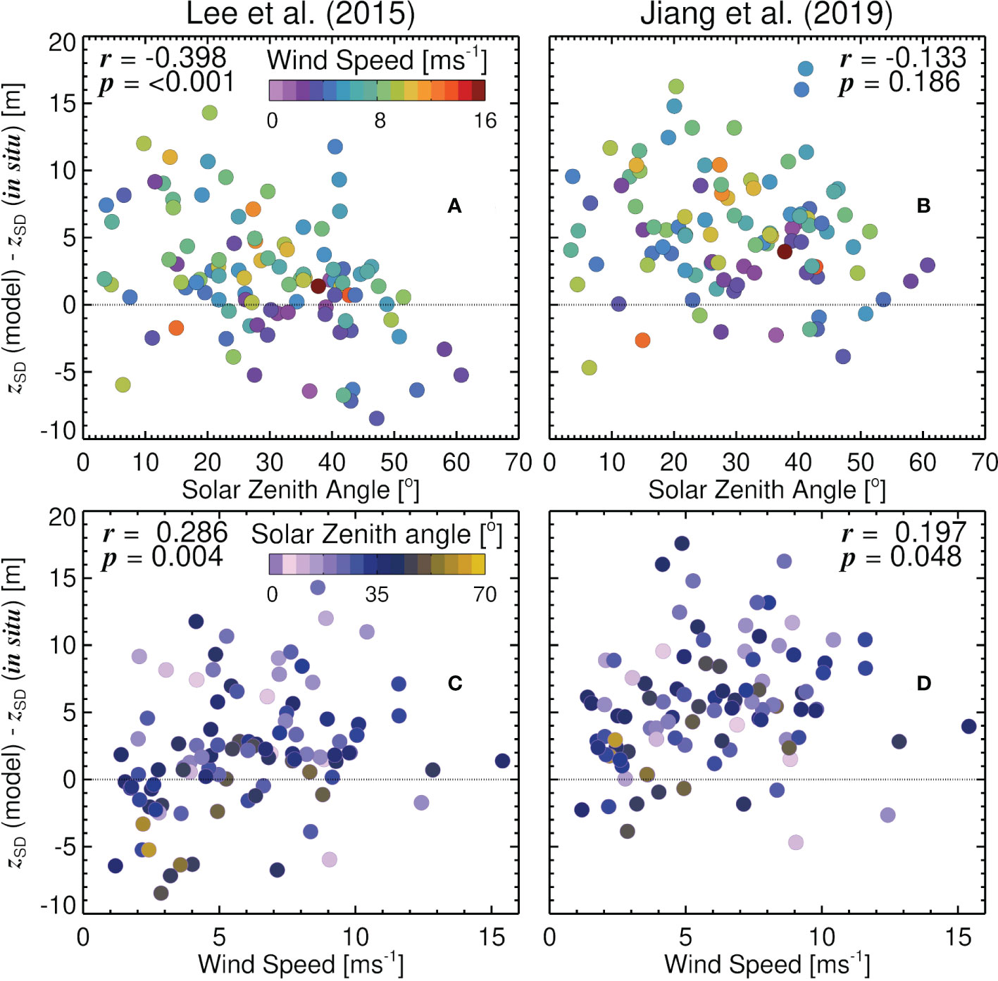
Figure 8 Differences (residuals) between R_rs-derived Secchi depth (z_SD) and in-situ z_SD, using the algorithms of Lee et al. (2015) (A, C) and Jiang et al. (2019) (B, D), plotted as a function of solar zenith angle (θ) (A, B) and wind speed (w_s) (C, D). Dotted line represents residuals of zero.

$\begin{array}{ll}{z}_{SD}=\frac{1}{\omega \min (K_d(\lambda ))}\text{ln}\left(\frac{\left|0.14-R_{rs}^{pc}\right|}{C_t^r}\right),& (3)\end{array}$

where $R_{rs}^{pc}$ represents remote sensing reflectance at the corresponding wavelength to min(K_d(λ)), $C_t^r$ is the threshold contrast for sighting a white Secchi disk, and ω converts min(K_d(λ)) to the sum of downwelling diffuse attenuation ($K_d^{tr}$) and upwelling diffuse attenuation ($K_T^{tr}$), in the transparent window. The Lee et al. (2015) algorithm fixes ω at 2.5, whereas the Jiang et al. (2019)algorithm has a variable ω, itself dependent on θ according to

$\begin{array}{ll}\omega =1+\frac{1.04{(1+5.4u)}^{0.5}}{1/{(1-\frac{sin{(\theta )}^2}{n_w{}^2})}^{0.5}},& (4)\end{array}$

where u is the ratio of the backscattering coefficient to the sum of absorption and backscattering coefficients (derived from R_rs following Lee et al. (2002; 2005; 2009)), and n_w is the refractive index of water (1.34). For the same backscattering and absorption coefficient, as θ increases, K_d(λ) increases in model of Lee et al. (2005) (used in both Jiang et al. (2019) and Lee et al. (2015) models), which subsequently decreases z_SD in Eq. 3. However, in the Jiang et al. (2019) algorithm, as θ increases, ω decreases (Eq. 4), which counterbalances the increase in (K_d(λ)) with θ. The resulting effect is that z_SD estimated using the Jiang et al. (2019) algorithm is less dependent on θ than for the Lee et al. (2015) model.

Differences (residuals) between the Lee et al. (2015) and Jiang et al. (2019) algorithms, and the in-situ z_SD data, were also found to be positively correlated with wind speed (Table 5 and Figure 8). At very low wind speed (<3 ms⁻¹), there is better agreement between models and in-situ data, with δ closer to zero (δ = −1.03 for Lee et al. (2015) and δ = 2.79 for Jiang et al. (2019)). These biases increased with increasing wind speed (Figure 8) Neither models incorporate a dependency of z_SD on wind speed, but our results are broadly consistent with theory of Preisendorfer (1986) that assumes an increase in wind speed causes a reduction in the apparent contrast of the disk at the surface, and a subsequent reduction in z_SD.

Though the Preisendorfer (1986) and Lee et al. (2015) Secchi disk theory define contrast differently, the Preisendorfer (1986) approach could be used to introduce some relationship between contrast and wind speed in the theory of Lee et al. (2015). The inherent contrast (C₀) is defined not as a relative difference in irradiance reflectance between the disk and the surrounding water (as in Preisendorfer, 1986), but as an absolute difference between the radiance reflectance of the disk (r₀) and the surrounding water ($r_{\infty }$), such that

$\begin{array}{ll}{C}_0=\left|r_0-r_{\infty }\right|.& (5)\end{array}$

The derived theory states that the contrast is modified as the distance (z) from the observer to the disk increases, such that

$\begin{array}{ll}C(z)=C_0\exp (-(K_d^{tr}+K_T^{tr})z).& (6)\end{array}$

Following Preisendorfer (1986), a contrast reduction factor ($\stackrel{-}{{\tau }_0}$) could be introduced, such that Eq. 6 becomes

$\begin{array}{ll}C(z)=\stackrel{-}{{\tau }_0}{C}_0\exp (-(K_d^{tr}+K_T^{tr})z).& (7)\end{array}$

If we make the assumption that $\stackrel{-}{{\tau }_0}$ is controlled by wind speed (w_s), acknowledging that other factors (which may or may not covary with w_s) are likely to impact $\stackrel{-}{{\tau }_0}$, we could relate $\stackrel{-}{{\tau }_0}$ to w_s empirically. To do that, we define x(z)=C₀/C(z), and for z=z_SD, it follows that C(z_SD)=0.013. Then, as the measurement is made from above the surface, it has to include another contrast reduction factor due to surface reflection effects, leading to $x\left(z_{SD}\right)=x_{SD}=\left|0.14-R_{\mathit{\text{rs}}}\right|/0.013$ (see Section 4 of Lee et al., 2015). To have an operational expression to solve for $\stackrel{-}{{\tau }_0}$, we make the ratio of Secchi depth with (z_SD,ws) and without (z_SD,ws=0) wind, such that

$\begin{array}{ll}\frac{z_{SD,ws}}{z_{SD,ws=0}}=\frac{\text{ln}(\stackrel{-}{{\tau }_0}{x}_{SD})}{\text{ln}(x_{SD})}.& (8)\end{array}$

Rearranging the equation following some algebra, we obtain

$\begin{array}{ll}\stackrel{-}{{\tau }_0}=x_{SD}\frac{z_{SD,ws}}{z_{SD,ws=0}}-1,& (9)\end{array}$

and derive $\stackrel{-}{{\tau }_0}$ by making the assumption z_SD,ws=0 is equal to the Jiang et al. (2019) algorithm output, and z_SD,ws represents the in-situ data. Next we model $\stackrel{-}{{\tau }_0}$ as a function of wind speed (w_s) and z_SD,ws=0 (Jiang 531 et al. (2019) algorithm), according to

$\begin{array}{ll}\stackrel{-}{{\tau }_0}=q_0\exp [-q_1{w}_s(1+q_2{z}_{SD,ws=0})],& (10)\end{array}$

with the expression chosen carefully to follow the observed trend in which wind explains most of the variation, but it is modulated by z_SD,ws=0. Fitting of Eq. 10 to the data resulted in $q_0=0.901\left(0.805\leftrightarrow 0.998\right)$, $q_1=0.022\left(-0.007\leftrightarrow 0.051\right)$, and $q_2=0.03\left(-0.045\leftrightarrow 0.106\right)$. Once $\stackrel{-}{{\tau }_0}$ is known, z_SD,ws can be estimated from

$\begin{array}{ll}{z}_{SD,ws}=\frac{\text{ln}(\stackrel{-}{{\tau }_0}{x}_{SD})}{\text{ln}(x_{SD})}{z}_{SD,ws=0}.& (11)\end{array}$

Using the modelled z_SD,ws (Jiang et al., 2019) removes the significant positive correlation between wind speed and model residuals (r=−0.135, p=0.179) apparent in original (Jiang et al., 2019) algorithm (z_SD,ws=0, Figure 8D). Additional datasets are need to independently validate this approach, but it certainly offers a way to incorporate the influence of wind speed into the Secchi depth theory of Lee et al. (2015), and could be useful for standardising in-situ z_SD data to a common wind speed.

3.5 Experiences and recommendations from collecting optical measurements using historical techniques on AMT

Our experience of collecting Secchi depth and Forel-Ule colour data on the Atlantic Meridional Transect revealed a number of insights. With the exception of a few sceptical scientists on-board the ship, there were many (scientists and members of the ship’s crew) that loved visually inspecting the colour and clarity of the water using the Secchi disk and Forel-Ule colour scales (see acknowledgements). It was the only time of the day where these participants had the opportunity to visually connect and interact with the ocean. The AMT transect was the perfect cruise to do this, as it transects through a ranges of conditions, with the clarity and colour of the water changing (sometimes rapidly) over the duration of the cruise. Visually inspecting the water also resulted in an increased number of sightings of marine wildlife and oceanic phenomena, including (and to name a few) observations of dolphins, sharks, whales, dolphinfish, rays, penguins, squid, turtles, icebergs, all manner of seabirds, as well as some of the more negative features (e.g., marine litter). For some, this had a positive influence on mental health, important to consider when on-board a research vessel for an extended period of time. Considering the nature of the measurement of Secchi depth and Forel-Ule colour, in that the observer is intrinsically part of the measurement process, it was a useful activity for teaching the concepts of ocean colour and clarity to non-scientists, and scientists working on other aspects of oceanography, on the AMT cruises.

Despite these positives, it was evident that measuring the Secchi depth in oligotrophic waters is challenging. After unsuccessfully attempting to deploy a Secchi disk using the traditional technique (rope and weighted Secchi disk), hindered by the disk drifting quickly away from the vessel (which was kept stationary), we followed the recommendations of the late Marcel Wernand, who in his 2010 paper states “…the author recommends a reintroduction of the Secchi disc to expand the historical Secchi depth database to facilitate climate change research. One option is to mount a Secchi disc on an instrumental or CTD frame…” (Wernand, 2010, p5). Once the disk was mounted on the optics rig (Figure 2A) it became feasible to do the measurements, as part of routine data collection.

A major challenge with conducting Secchi depth measurements in oligotrophic waters, is the fact that the disk disappears at a depth far greater than in mesotrophic and eutrophic waters. The angular subtense of the disk’s radius ($\text{Φ}=r_{SD}/z_{SD}$, r_SD is the disk’s radius, the first order approximation of the MacLaurin expansion of the arctan function), for a 30 cm diameter disk at a z_SD of 50 m, is 0.003. To put this into perspective (and something that could easily be tested in inland water), the target viewed is equivalent to lowering a 1 cm diameter disk to 1.7 m. One solution could be to increase the disk size for oligotrophic waters. Although a 30 cm diameter disk is standard for measuring the Secchi depth in the ocean, Angelo Secchi himself used disks as big as 2.5 m in diameter in his early work (Pitarch et al., 2021), and others have modified the disk size to be smaller in more turbid waters (e.g., Brewin et al., 2019a). However, the exact impact of disk size on Secchi depth is still a matter of research (Hou et al., 2007). Another possible artefact of a very low angular subtense ($\text{Φ}$) in oligotrophic waters, could be an increasing impact of environmental factors on the detection threshold of the human eye (in air) seeing the disk, since the target is so small. Additionally, there may be other optical effects that occur, that are not currently accounted for in the theory. For example, with a very small target in a moving ocean, there may be some kind of adjacency effect, caused by the spectrum near the edge of the disk being a mixture of reflectance of the disk and the infinitely deep waters.

The dataset collected on AMT is freely available (Brewin et al., 2023), courtesy of the British Oceanographic Data Centre (BODC), for use in future research on the topic. In this paper, we have compared and evaluated broad relationships between historic and modern optical techniques for monitoring phytoplankton biomass. Future work could use these data to examine in greater detail the influence of varying concentrations of different optically-active constituents on the relationships between Secchi depth, Forel-Ule colour, R_rs, and Chl-a. For example, variations in coloured dissolved organic matter (CDOM) will have an impact on water colour, and consequently the relationships between bulk variables (Van der Woerd and Wernand, 2018). For some AMT cruises, underway CDOM absorption data (Dall’Olmo et al., 2017), as well as underway and profile particulate absorption and scattering measurements (Dall’Olmo et al., 2012; Brewin et al., 2016; Tilstone et al., 2021), have been collected, and could be useful for studying relationships between Secchi depth, Forel-Ule colour, R_rs, and Chl-a.

Measuring PAR on a profiling package and the Secchi depth from a large oceanographic vessel could lead to cases of ship shadow. For PAR, this was somewhat minimised by only using profiles where depth and log(PAR) were tightly correlated and (where possible) deploying the profiling package on the sunny side of the vessel. Our K_d values for oligotrophic waters (varying between 0.02 – 0.08) are consistent with values from satellite data in the region (e.g., Son and Wang, 2015) and consistent with BGC-Argo float data (see Demeaux and Boss (2022)). AMT K_d data also agreed well with K_d estimates from a BGC-Argo float WMO:3902121 in the South Atlantic gyre, (results not shown).

Another factor that may influence relationships between Secchi depth, Forel-Ule colour, R_rs, and Chl-a, are shifts in the community composition of phytoplankton. It is well know that the chl-specific absorption and backscattering coefficients vary with phytoplankton community composition (e.g., Ciotti et al., 2002; Sathyendranath et al., 2004; Kostadinov et al., 2010; Brewin et al., 2011; Devred et al., 2011; Brewin et al., 2012a; Brewin et al., 2019b). Although the median ratio of Secchi-depth to mixed-layer depth (computed using temperature criterion of de Boyer Montégut et al. (2004)) was found to be 0.49 (standard deviation 0.44), suggesting on average the mixed-layer depth was twice that of the Secchi depth, there were a few cases where the Secchi depth was shallower than the mixed-layer depth. Vertical variability in Chl-a and phytoplankton community structure in the region (Mojica et al., 2015), and within the Secchi depth layer, may exist (e.g., in very clear waters, with very shallow mixed-layers) which may complicate relationships between Secchi depth, Forel-Ule colour, R_rs, and Chl-a.

We chose to use surface Chl-a, rather than depth-averaged Chl-a within the Secchi depth layer, in our analysis, as it has been recommended by the community to use surface Chl-a when developing surface optical models (Sathyendranath et al., 2019; Lee et al., 2020), and it allowed us to compare relationships in our dataset with earlier algorithms (Boyce et al., 2012; Lee et al., 2018c). However, datasets on vertical variations in Chl-a and community composition (e.g. through flow cytometry and HPLC analysis) have been collected on AMT cruises, and could be useful for studying impact of vertical variability in water constituents on proposed models. Future efforts in collecting vertically-resolved inherent optical properties, alongside Secchi depth and FU measurements, would help further. Considering issues with direct observations of Forel-Ule colour of infinite waters not resolving subtle variations in low Chl-a in oligotrophic waters, we recommend measuring Forel-Ule colour in oligotrophic waters using the colour of the Secchi disk at 1/2z_SD.

4 Summary

On four AMT cruises (23, 25, 26 and 28), we collected a dataset of both modern (radiometric) and traditional (Secchi depth and Forel-Ule colour) measurements of ocean clarity and colour, together with in-situ measurements of Chl-a, with the aim to evaluate relationships between historic and modern methods for monitoring phytoplankton biomass, and evaluate satellite ocean colour remote-sensing algorithms, two key goals of the AMT programme. Historic and modern optical measurements were in good agreement and consistent with current understanding, with the Secchi depth inversely correlated to the Forel-Ule colour, beam and diffuse attenuation, and positively correlated to the euphotic depth and R_rs(MB)/R_rs(G). The relationship between Secchi depth and Forel-Ule on AMT was also in good agreement with historical data, but only when using data of the Forel-Ule colour of infinite water (estimated using Pitarch (2017)), rather than the Forel-Ule colour of the Secchi disk at half the Secchi depth. R_rs(MB)/R_rs(G) explained the highest amount of variance in Chl-a (89%), closely followed by the Secchi depth (85%) and the Forel-Ule colour (71-81%, depending on scale used). Overall, algorithms that predict Chl-a from these optical proxies were found to perform well, with some systematic differences. Algorithms that estimate Forel-Ule and Secchi depth from remote sensing reflectance were found to be in good agreement with the in-situ data, albeit with a positive bias (2.0 - 5.4 m, ~8-22%) in Secchi depth, and differences in performance depending on which Forel-Ule scale and method were used (infinite colour or colour of water above disk at 1/2z_SD). The impact of different environmental variables on relationships between optical proxies was investigated, and varied depending on the optical proxies analysed. We found wind speed to impact the estimation of z_SD, and proposed a path forward to include the effect of wind in current Secchi depth theory, based on the classical work of Preisendorfer (1986). We highlight some of the benefits and challenges in collecting optical measurements using traditional methods on AMT, and highlight future directions for research. Our dataset is made publicly available to support the research community (see Brewin et al., 2023).

Data availability statement

The dataset used for this study is openly available through the British Oceanographic Data Centre (see https://doi.org/10.5285/f3198e10-faf3-1525-e053-6c86abc0d2f6).

Author contributions

RB and GD organised and participated in the collection of all the Secchi disk and Forel-Ule colour data. RB, GD, and GT organised and participated in the collection of all modern optical datasets used (e.g., radiometry). RB wrote an initial plan for the paper with input from GD, JP, and HW. JL and XS contributed to data processing and figure production. RB and JP synthesised the data, ran the analysis and prepared the figures. RB wrote the first version of the manuscript, with input from JP. All authors contributed to the article and approved the submitted version.

Funding

This work was supported by grants from the European Space Agency (ESA), including the Changing Earth Science Network initiative funded by the STSE programme (DECIPHER project), AMT4SentinelFRM (ESRIN/RFQ/3-14457/16/I-BG) and AMT4OceanSatFlux (4000125730/18/NL/FF/gp). Additional support from the UK National Centre for Earth Observation is acknowledged. The work was supported by UK Natural Environment Research Council (NERC) National Capability funding for AMT to Plymouth Marine Laboratory. AMT is funded by the NERC through its National Capability Long-term Single Centre Science Programme, Climate Linked Atlantic Sector Science (grant number NE/R015953/1). This study contributes to the international IMBeR project and is contribution number 384 of the AMT programme. RB is funded by a UKRI Future Leader Fellowship (MR/V022792/1).

Acknowledgments

We thank Marcel Wernand for providing Forel-Ule scale used on AMT25, AMT26 and AMT28, and for his support for collecting Forel-Ule and Secchi depth data on AMT. We are indebted to the all the scientists, the captain’s and crew of the RRS James Clark Ross, on AMT23, AMT25, AMT26, and AMT28, who helped make this work happen. Especially those who were kind enough to come out on deck at the noon station, look at the ocean, and help us collect the Forel-Ule and Secchi depth data, specific thanks goes to: Arwen Bargery, Carolina Beltran, Kimberley Bird, Ian Brown, Catherine Burd, Priscilla Lange, Phyllis Lam, Ankita Misra, Catherine Mitchell, Mónica Moniz, Clifford Mullaney, Francesco Nencioli, John O’Duffy, Emanuele Organelli, Paul Provost, Rafael Rasse, Andy Rees, Nick Rundle, Bita Sabbaghzadeh, Chata Seguro, Charlotte Smith, Tim Smyth, Madeline Steer, Glen Tarran, Robyn Tuerena, Natalie Wager, and Simon Wright. We thank Tom Jackson for help in data transfer and Afonso Ferreira and Andreia Tracana for help filtering water for HPLC analysis on AMT28. We thank Arwen Bargery, Priscilla Lange and Phyllis Lam, for use of photos in Figure 2. We thank all those that contributed to the CalCOFI and NODC datasets.

Conflict of interest

The authors declare that the research was conducted in the absence of any commercial or financial relationships that could be construed as a potential conflict of interest.

The handling editor VB declared a past co-authorship with the authors RB and XS.

Publisher’s note

All claims expressed in this article are solely those of the authors and do not necessarily represent those of their affiliated organizations, or those of the publisher, the editors and the reviewers. Any product that may be evaluated in this article, or claim that may be made by its manufacturer, is not guaranteed or endorsed by the publisher.

References

Aiken J., Rees N., Hooker S., Holligan P., Bale A., Robins D., et al. (2000). The Atlantic Meridional Transect: Overview and synthesis of data. Prog. Oceanography 45, 257–312. doi: 10.1016/S0079-6611(00)00005-7

CrossRef Full Text | Google Scholar

Antoine D., Morel A., Gordon H. R., Banzon V. F., Evans R. H. (2005). Bridging Ocean Color observations of the 1980s and 2000s in search of long-term trends. J. Geophysical Research: Oceans 110, 1–22. doi: 10.1029/2004JC002620

CrossRef Full Text | Google Scholar

Behrenfeld M. (2011). Uncertain future for ocean algae. Nat. Climate Change 1, 33–34. doi: 10.1038/nclimate1069

CrossRef Full Text | Google Scholar

Behrenfeld M. J. (2014). Climate-mediated dance of the plankton. Nat. Climate Change 4, 880–887. doi: 10.1038/nclimate2349

CrossRef Full Text | Google Scholar

Behrenfeld M. J., O’Malley R. T., Siegel D. A., McClain C. R., Sarmiento J. L., Feldman G. C., et al. (2006). Climate-driven trends in contemporary ocean productivity. Nature 444, 752–755. doi: 10.1038/nature05317

PubMed Abstract | CrossRef Full Text | Google Scholar

Boyce D. G., Dowd M., Lewis M. R., Worm B. (2014). Estimating global chlorophyll changes over the past century. Prog. Oceanography 122, 163–173. doi: 10.1016/j.pocean.2014.01.004

CrossRef Full Text | Google Scholar

Boyce D. G., Lewis M. R., Worm B. (2010). Global phytoplankton decline over the past century. Nature 466, 591–596. doi: 10.1038/nature09268

PubMed Abstract | CrossRef Full Text | Google Scholar

Boyce D. G., Lewis M., Worm B. (2012). Integrating global chlorophyll data from 1890 to 2010. Limnology Oceanography Methods 10, 840–852. doi: 10.4319/lom.2012.10.840

CrossRef Full Text | Google Scholar

Brewin R. J. W., Brewin T. G., Phillips J., Rose S., Abdulaziz A., Wimmer W., et al. (2019a). A printable device for measuring clarity and colour in lake and nearshore waters. Sensors 9, 1–26. doi: 10.3390/s19040936

CrossRef Full Text | Google Scholar

Brewin R. J. W., Ciavatta S., Sathyendranath S., Skákala J., Bruggeman J., Ford D., et al. (2019b). The influence of temperature and community structure on light absorption by phytoplankton in the north Atlantic. Sensors 19, 1–25. doi: 10.3390/s19194182

CrossRef Full Text | Google Scholar

Brewin R. J. W., Dall’Olmo G., Gittings J., Sun X., Lange P. K., Raitsos D. E., et al. (2022). A conceptual approach to partitioning a vertical profile of phytoplankton biomass into contributions from two communities. J. Geophysical Researech: Oceans 127, e2021JC018195. doi: 10.1029/2021JC018195

CrossRef Full Text | Google Scholar

Brewin R. J. W., Dall’Olmo G., Pardo S., van Dongen-Vogel V., Boss E. S. (2016). Underway spectrophotometry along the Atlantic Meridional Transect reveals high performance in satellite chlorophyll retrievals. Remote Sens. Environ. 183, 82–97. doi: 10.1016/j.rse.2016.05.005

CrossRef Full Text | Google Scholar

Brewin R. J. W., Dall’Olmo G., Sathyendranath S., Hardman-Mountford N. J. (2012a). Particle backscattering as a function of chlorophyll and phytoplankton size structure in the open-ocean. Optics Express 20, 17632–17652. doi: 10.1364/OE.20.017632

PubMed Abstract | CrossRef Full Text | Google Scholar

Brewin R. J. W., Devred E., Sathyendranath S., Lavender S. J., Hardman-Mountford N. J. (2011). Model of phytoplankton absorption based on three size classes. Appl. Optics 50, 4535–4549. doi: 10.1364/AO.50.004535

CrossRef Full Text | Google Scholar

Brewin R. J. W., Hirata T., Hardman-Mountford N. J., Lavender S., Sathyendranath S., Barlow R. (2012b). The influence of the Indian ocean dipole on interannual variations in phytoplankton size structure as revealed by Earth Observation. Deep Sea Res. II 77-80, 117–127. doi: 10.1016/j.dsr2.2012.04.009

CrossRef Full Text | Google Scholar

Brewin R. J.W., Pitarch J., Dall'Olmo G., van der Woerd H. J., Lin J., Sun X., Tilstone G. H. (2023). Modern and traditional optical measurements, and environmental data, collected on four Atlantic Meridional Transect cruises between 2013 and 2018. NERC EDS British Oceanographic Data Centre NOC. doi: 10.5285/f3198e10-faf3-1525-e053-6c86abc0d2f6

CrossRef Full Text | Google Scholar

Brewin R. J. W., Tilstone G., Jackson T., Cain T., Miller P., Lange P. K., et al. (2017). Modelling size-fractionated primary production in the Atlantic ocean from remote sensing. Prog. Oceanography 158, 130–149. doi: 10.1016/j.pocean.2017.02.002

CrossRef Full Text | Google Scholar

Brotas V., Tarran G. A., Veloso V., Brewin R. J. W., Woodward E. M. S., Airs R., et al. (2022). Complementary approaches to assess phytoplankton groups and size classes on a long transect in the Atlantic ocean. Front. Mar. Sci. 8. doi: 10.3389/fmars.2021.682621

CrossRef Full Text | Google Scholar

Busch J. A., Bardaji R., Ceccaroni L., Friedrichs A., Piera J., Simon C., et al. (2016). Citizen bio-optical observations from coast-and ocean and their compatibility with ocean colour satellite measurements. Remote Sens. 8, 1–19. doi: 10.3390/rs8110879

CrossRef Full Text | Google Scholar

Campbell J. W. (1995). The lognormal distribution as a model for bio-optical variability in the sea. J. Geophysical Res. 100 (C7), 13237–13254. doi: 10.1029/95JC00458

CrossRef Full Text | Google Scholar

Chai F., Johnson K. S., Claustre H., Xing X., Wang Y., Boss E., et al. (2020). Monitoring ocean biogeochemistry with autonomous platforms. Nat. Rev. Earth Environ. 1, 315–326. doi: 10.1038/s43017-020-0053-y

CrossRef Full Text | Google Scholar

Chassot E., Bonhommeau S., Dulvy N. K., Mélin F., Watson R., Gascuel D., et al. (2010). Global marine primary production constrains fisheries catches. Ecol. Lett. 13, 495–505. doi: 10.1111/j.1461-0248.2010.01443.x

PubMed Abstract | CrossRef Full Text | Google Scholar

Ciotti A. M., Lewis M. R., Cullen J. J. (2002). Assessment of the relationships between dominant cell size in natural phytoplankton communities and the spectral shape of the absorption coefficient. Limnology Oceanography 47, 404–417. doi: 10.4319/lo.2002.47.2.0404

CrossRef Full Text | Google Scholar

Dall’Olmo G., Boss E., Behrenfeld M., Westberry T. K. (2012). Particulate optical scattering coefficients along an Atlantic Meridional Transect. Optics Express 20, 21532–21551. doi: 10.1364/OE.20.021532

PubMed Abstract | CrossRef Full Text | Google Scholar

Dall’Olmo G., Brewin R. J. W., Nencioli F., Organelli E., Lefering I., McKee D., et al. (2017). Determination of the absorption coefficient of chromophoric dissolved organic matter from underway spectrophotometry. Optics Express 25, A1079–A1095. doi: 10.1364/OE.25.0A1079

PubMed Abstract | CrossRef Full Text | Google Scholar

de Boyer Montégut C., Madec G., Fischer A. S., Lazar A., Iudicone D. (2004). Mixed layer depth over the global ocean: An examination of profile data and a profile-based climatology. J. Geophysical Reserach: Oceans 109, 1–20. doi: 10.1029/2004JC002378

CrossRef Full Text | Google Scholar

Demeaux C. B., Boss E. (2022). Validation of remote-sensing algorithms for diffuse attenuation of downward irradiance using BGC-argo floats. Remotre Sens. 14, 4500. doi: 10.3390/rs14184500

CrossRef Full Text | Google Scholar

Devred E., Sathyendranath S., Stuart V., Platt T. (2011). A three component classification of phytoplankton absorption spectra: Applications to ocean-colour data. Remote Sens. Environ. 115, 2255–2266. doi: 10.1016/j.rse.2011.04.025

CrossRef Full Text | Google Scholar

Dow K., Downing T. E. (2011). The atlas of climate change: mapping the world’s greatest challenge (Univ of California Press, Oakland, California).

Google Scholar

Dutkiewicz S., Hickman A. E., Jahn O., Henson S., Beaulieu C., Moneir E. (2019). Ocean colour signature of climate change. Nat. Commun. 10, 578. doi: 10.1038/s41467-019-08457-x

PubMed Abstract | CrossRef Full Text | Google Scholar

Falkowski P. G. (2012). Ocean science: The power of plankton. Nature 483, S17–S20. doi: 10.1038/483s17a

PubMed Abstract | CrossRef Full Text | Google Scholar

Falkowski P. G., Wilson C. (1992). Phytoplankton productivity in the North Pacific ocean since 1900 and implications for absorption of anthropogenic co₂. Nature 358, 741–743. doi: 10.1038/358741a0

CrossRef Full Text | Google Scholar

Field C. B., Behrenfeld M. J., Randerson J. T., Falkowski P. G. (1998). Primary production of the biosphere: integrating terrestrial and oceanic components. Science 281, 237–240. doi: 10.1126/science.281.5374.237

PubMed Abstract | CrossRef Full Text | Google Scholar

Forel F. A. (1890). “Une nouvelle forme de la gamme de couleur pour l’étude de l’eau des lacs,” in Archives des sciences physiques et Naturelles/Société de physique et d’Histoire naturelle de genève, vol. 6. , 25.

Google Scholar

GCOS (2011). “Systematic observation requirements from satellite-based data products for climate,” in Tech. rep (7 bis, avenue de la Paix, CH-1211 Geneva 2, Switzerland: World Meteorological Organisation (WMO).

Google Scholar

Gregg W. W., Conkright M. E. (2002). Decadal changes in global ocean chlorophyll. Geophysical Res. Lett. 29, 20–1–20–4. doi: 10.1029/2002GL014689

CrossRef Full Text | Google Scholar

Henson S. A. (2014). Slow science: the value of long ocean biogeochemistry records. Philos. Trans. R. Soc. A 372, 1–22. doi: 10.1098/rsta.2013.0334

CrossRef Full Text | Google Scholar

Henson S. A., Cael B. B., Allen S. R., Dutkiewicz S. (2021). Future phytoplankton diversity in a changing climate. Nat. Commun. 12, 1–8. doi: 10.1038/s41467-021-25699-w

PubMed Abstract | CrossRef Full Text | Google Scholar

Henson S. A., Sarmiento J. L., Dunne J. P., Bopp L., Lima I., Doney S. C., et al. (2010). Detection of anthropogenic climate change in satellite records of ocean chlorophyll and productivity. Biogeosciences 7, 621–640. doi: 10.5194/bg-7-621-2010

CrossRef Full Text | Google Scholar

Hou W., Lee Z., Weidemann A. D. (2007). Why does the Secchi disk disappear? an imaging perspective. Optics Express 15, 2791–2802. doi: 10.1364/OE.15.002791

PubMed Abstract | CrossRef Full Text | Google Scholar

Hu C., Lee Z., Franz B. (2012). Chlorophyll a algorithms for oligotrophic oceans: A novel approach based on three-band reflectance difference. J. Geophysical Res. 117, C01011. doi: 10.1029/2011JC007395

CrossRef Full Text | Google Scholar

IPCC (2019). “IPCC Special Report on the Ocean and Cryosphere in a Changing Climate," Eds, Pörtner H.-O., Roberts D.C., Masson-Delmotte V., Zhai P., Tignor M., Poloczanska E., et al. Cambridge University Press, Cambridge, UK and New York, NY, USA, 755 pp. doi: 10.1017/9781009157964.

CrossRef Full Text | Google Scholar

Jiang D., Matsushita B., Setiawan F., Vundo A. (2019). An improved algorithm for estimating the Secchi disk depth from remote sensing data based on the new underwater visibility theory. ISPRS J. Photogrammetry Remote Sens. 152, 13–23. doi: 10.1016/j.isprsjprs.2019.04.002

CrossRef Full Text | Google Scholar

Kostadinov T. S., Siegel D. A., Maritorena S. (2010). Global variability of phytoplankton functional types from space: assessment via the particle size distribution. Biogeosciences 7, 3239–3257. doi: 10.5194/bgd-7-4295-2010

CrossRef Full Text | Google Scholar

Lee Z., Arnone R., Boyce D., Franz B., Greb S., Hu C., et al. (2018a). Global water clarity: Continuing a century-long monitoring. Eos 99. doi: 10.1029/2018EO097251

PubMed Abstract | CrossRef Full Text | Google Scholar

Lee Z., Carder K. L., Arnone R. A. (2002). Deriving inherent optical properties from water color: a multiband quasi-analytical algorithm for optically deep waters. Appl. Optics 41, 5755–5772. doi: 10.1364/AO.41.005755

CrossRef Full Text | Google Scholar

Lee Z., Du K., Arnone R. (2005). A model for the diffuse attenuation coefficient of downwelling irradiance. J. Geophysical Res. 110, C02016. doi: 10.1029/2004JC002275

CrossRef Full Text | Google Scholar

Lee Z., Lubac B., Werdell P. J., Arnone R. (2009). An update of the quasi-analytical algorithm (QAA_v5). In: Tech. rep (International Ocean Colour Coordinating Group (IOCCG). Available at: http://www.ioccg.org/groups/software.html (Accessed assessed 07/11/2022).

Google Scholar

Lee Z., Shang S., Du K., Liu B., Lin G., Wei J., et al. (2018b). Enhance field water-color measurements with a Secchi disk and its implication for fusion of active and passive ocean-color remote sensing. Appl. Optics 57, 3463–3473. doi: 10.1364/AO.57.003463

CrossRef Full Text | Google Scholar

Lee Z., Shang S., Du K., Wei J. (2018c). Resolving the long-standing puzzles about the observed Secchi depth relationships. Limnology Oceanography 63, 2321–2336. doi: 10.1002/lno.10940

CrossRef Full Text | Google Scholar

Lee Z., Shang S., Hu C., Du K., Weidemann A., Hou W., et al. (2015). Secchi disk depth: A new theory and mechanistic model for underwater visibility. Remote Sens. Environ. 169, 139–149. doi: 10.1016/j.rse.2015.08.002

CrossRef Full Text | Google Scholar

Lee Z., Wang Y., Yu X., Shang S., Luis K. (2020). Evaluation of forward reflectance models and empirical algorithms for chlorophyll concentration of stratified waters. Appl. Optics 59, 9340–9352. doi: 10.1364/AO.400070

CrossRef Full Text | Google Scholar

Lee Z., Du K., Voss K. J., Zibordi G., Lubac B., Arnone R., et al. (2011). An inherent-optical-property-centered approach to correct the angular effects in water-leaving radiance. Appl. Optics 50, 3155–3167. doi: 10.1364/AO.50.003155

CrossRef Full Text | Google Scholar

Lewis M. R., Kuring N., Yentsch C. (1988). Global patterns of ocean transparency: Implications for the new production of the open ocean. Jounral Geophysical Res. 93, 6847–6856. doi: 10.1029/JC093iC06p06847

CrossRef Full Text | Google Scholar

Lin J., Dall’Olmo G., Tilstone G. H., Brewin R. J. W., Vabson V., Ansko I., et al. (2022). Derivation of uncertainty budgets for continuous above-water radiometric measurements along an Atlantic Meridional Transect. Optics Express. doi: 10.1364/OE.470994

CrossRef Full Text | Google Scholar

Longhurst A., Sathyendranath S., Platt T., Caverhill C. (1995). An estimate of global primary production in the ocean from satellite radiometer data. J. Plankton Res. 17, 1245–1271. doi: 10.1093/plankt/17.6.1245

CrossRef Full Text | Google Scholar

Mackas D. L. (2011). Does blending of chlorophyll data bias temporal trend? Nature 472, E4–E5. doi: 10.1038/nature09951

PubMed Abstract | CrossRef Full Text | Google Scholar

Malthus T. J., Ohmsen R., van der Woerd H. J. (2020). An evaluation of citizen science smartphone apps for inland water quality assessment. Remote Sensing. 12, 1578. doi: 10.3390/rs12101578

CrossRef Full Text | Google Scholar

Markwardt C. B. (2008). “Non-linear least squares fitting in IDL with MPFIT,” in Proceedings of the astronomical data analysis software and systems XVIII, vol. 411 . Eds. Bohlender D., Dowler P., Duran D. (Quebec, Canada: Astronomical Society of the Pacific, San Francisco).

Google Scholar

Martinez E., Antoine D., D’ortenzio F., Gentili B. (2009). Climate-driven basin-scale decadal oscillations of oceanic phytoplankton. Science 326, 1253–1256. doi: 10.1126/science.1177012

PubMed Abstract | CrossRef Full Text | Google Scholar

McQuatters-Gollop A., Reid P., Edwards M., Burkill P. H., Castellani C., Batten S., et al. (2011). Is there a decline in marine phytoplankton? Nature 472, E6–E7. doi: 10.1038/nature09950

PubMed Abstract | CrossRef Full Text | Google Scholar

Mobley C. D. (1999). Estimation of the remote-sensing reflectance from above-surface measurements. Appl. Optics 38, 7442–7455. doi: 10.1364/AO.38.007442

CrossRef Full Text | Google Scholar

Mojica K. D. A., van de Poll W. H., Kehoe M., Huisman J., Timmermans K. R., Buma A. G. J., et al. (2015). Phytoplankton community structure in relation to vertical stratification along a north-south gradient in the northeast Atlantic ocean. Limnolology Oceanography 60, 1498–1521. doi: 10.1002/lno.10113

CrossRef Full Text | Google Scholar

Moré J. (1978). “The levenberg-marquardt algorithm: implementation and theory,” in Numerical analysis (Berlin: Springer-Verlag).

Google Scholar

Morel A., Huot Y., Gentili B., Werdell P. J., Hooker S. B., Franz B. A. (2007). Examining the consistency of products derived from various Ocean Color sensors in open ocean (case 1) waters in the perspective of a multi-sensor approach. Remote Sens. Environ. 111, 69–88. doi: 10.1016/j.rse.2007.03.012

CrossRef Full Text | Google Scholar

Morel A., Prieur L. (1977). Analysis of variations in Ocean Color. Limnology Oceanography 22, 709–722. doi: 10.4319/lo.1977.22.4.0709

CrossRef Full Text | Google Scholar

NASA (2010). Ocean Color chlorophyll (OC) v6. In: Tech. rep. Available at: https://oceancolor.gsfc.nasa.gov/reprocessing/r2009/ocv6/ (Accessed 23/11/2022).

Google Scholar

Novoa S., Wernand M., van der Woerd H. J. (2015). WACODI: A generic algorithm to derive the intrinsic color of natural waters from digital images. Limnology Oceanography Methods 13, 697–711. doi: 10.1002/lom3.10059\

CrossRef Full Text | Google Scholar

Novoa S., Wernand M. R., van der Woerd H. J. (2014). The modern Forel-Ule scale: a ‘do-it-yourself’ colour comparator for water monitoring. J. Eur. Optical Soc. - Rapid Publications 9, 1–10. doi: 10.2971/jeos.2014.14025

CrossRef Full Text | Google Scholar

O’Reilly J. E., Maritorena S., Mitchell B. G., Siegel D. A., Carder K. L., Garver S. A., et al. (1998). Ocean chlorophyll algorithms for SeaWiFS. J. Geophysical Res. 103, 24,937–24,953. doi: 10.1029/98JC02160

CrossRef Full Text | Google Scholar

Pitarch J. (2017). Biases in Ocean Color over a Secchi disk. Optics Express 25, A1124–A1131. doi: 10.1364/OE.25.0A1124

PubMed Abstract | CrossRef Full Text | Google Scholar

Pitarch J. (2020). A review of Secchi’s contribution to marine optics and the foundation of Secchi disk science. Oceanography 33, 26–37. doi: 10.5670/oceanog.2020.301

CrossRef Full Text | Google Scholar

Pitarch J., Bellacicco M., Marullo S., van der Woerd H. J. (2021). Global maps of Forel–Ule index, hue angle and Secchi disk depth derived from 21 years of monthly ESA ocean colour climate change initiative data. Earth System Sci. Data 13, 481–490. doi: 10.5194/essd-13-481-2021

CrossRef Full Text | Google Scholar

Pitarch J., Bellacicco M., Organelli E., Volpe G., Colella S., Vellucci V., et al. (2020). Retrieval of particulate backscattering using field and satellite radiometry: Assessment of the QAA algorithm. Remote Sens. 12, 77. doi: 10.3390/rs1201007

CrossRef Full Text | Google Scholar

Pitarch J., van der Woerd H. J., Brewin R. J. W., Zielinski O. (2019). Optical properties of Forel-Ule water types deduced from 15 years of global satellite Ocean Color observations. Remote Sens. Environ. 231, 111249. doi: 10.1016/j.rse.2019.111249

CrossRef Full Text | Google Scholar

Pitarch J., Vanhellemont Q. (2021). The QAA-RGB: A universal three-band absorption and backscattering retrieval algorithm for high resolution satellite sensors. development and implementation in ACOLITE. Remote Sens. Environ. 265, 112667. doi: 10.1016/j.rse.2021.112667

CrossRef Full Text | Google Scholar

Pope R., Fry E. (1997). Absorption spectrum (380-700 nm) of pure water. II. integrating cavity measurements. Appl. Optics 36, 8710–8723. doi: 10.1364/AO.36.008710

CrossRef Full Text | Google Scholar

Preisendorfer R. W. (1986). Secchi disk science: Visual optics of natural waters. Limnology Oceanography 31, 909–926. doi: 10.4319/lo.1986.31.5.0909

CrossRef Full Text | Google Scholar

Raitsos D. E., Pradhan Y., Lavender S. J., Hoteit I., McQuatters-Gollop A., Reid P. C., et al. (2014). From silk to satellite: half a century of ocean colour anomalies in the northeast Atlantic. Global Change Biol. 20, 2117–2123. doi: 10.1111/gcb.12457

CrossRef Full Text | Google Scholar

Rasse R., Dall’Olmo G., Graff J., Westberry T. K., van Dongen-Vogels V., Behrenfeld M. J. (2017). Evaluating optical proxies of particulate organic carbon across the surface Atlantic ocean. Front. Mar. Sci. 4, 1–18. doi: 10.3389/fmars.2017.00367

CrossRef Full Text | Google Scholar

Rees A. P., Nightingale P. D., Poulton A. J., Smyth T., Tarran G. A., Tilstone G. (2017). The Atlantic Meridional Transect programme, (1995–2016). Prog. Oceanography 158, 3–18. doi: 10.1016/j.pocean.2017.05.004

CrossRef Full Text | Google Scholar

Rees A. P., Robinson C., Smyth T., Aiken J., Nightingale P., Zubkov M. (2015). 20 years of the Atlantic Meridional Transect – AMT. Limnology Oceanography Bull. 24, 101–127. doi: 10.1002/lob.10069

CrossRef Full Text | Google Scholar

Robinson C., Poulton A. J., Holligan P. M., Baker A. R., Forster G., Gist N., et al. (2006). The Atlantic Meridional Transect (AMT) programme: a contextual view 1995-2005. Deep Sea Res. II 53, 1485–1515. doi: 10.1016/j.dsr2.2006.05.015

CrossRef Full Text | Google Scholar

Ruddick K. G., De Cauwer V., Park Y.-J., Moore G. (2006). Seaborne measurements of near infrared water-leaving reflectance: The similarity spectrum for turbid waters. Limnology Oceanography 51, 1167–1179. doi: 10.4319/lo.2006.51.2.1167

CrossRef Full Text | Google Scholar

Rykaczewski R., Dunne J. (2011). A measured look at ocean chlorophyll trends. Nature 472, E5–E6. doi: 10.1038/nature0995

PubMed Abstract | CrossRef Full Text | Google Scholar

Sathyendranath S., Brewin R. J. W., Brockmann C., Brotas V., Calton B., Chuprin A., et al. (2019). An ocean-colour time series for use in climate studies: The experience of the Ocean-Colour Climate Change Initiative (OC-CCI). Sensors 19, 4285. doi: 10.3390/s19194285

PubMed Abstract | CrossRef Full Text | Google Scholar

Sathyendranath S., Brewin R. J. W., Jackson T., Mélin F., Platt T. (2017). Ocean-colour products for climate-change studies: What are their ideal characteristics? Remote Sens. Environ. 203, 125–138. doi: 10.1016/j.rse.2017.04.017

CrossRef Full Text | Google Scholar

Sathyendranath S., Watts L., Devred E., Platt T., Caverhill C., Maass H. (2004). Discrimination of diatoms from other phytoplankton using ocean-colour data. Mar. Ecol. Prog. Ser. 272, 59–68. doi: 10.3354/meps272059

CrossRef Full Text | Google Scholar

Secchi P. A. (1864). Relazione delle esperienze fatte a bordo della pontificia pirocorvetta l’Immacolata concezione per determinare la trasparenza del mare; memoria del P. A. Secchi. Il Nuovo Cimento 1855-1868) 20, 205–238. doi: 10.1007/BF02726911

CrossRef Full Text | Google Scholar

Siegel D. A., Franz B. A. (2010). Century of phytoplankton change. Nature 466, 569–571. doi: 10.1038/466569a

PubMed Abstract | CrossRef Full Text | Google Scholar

Son S., Wang M. (2015). Diffuse attenuation coefficient of the photosynthetically available radiation K_d(par) for global open ocean and coastal waters. Remote Sens. Environ. 159, 250–258. doi: 10.1016/j.rse.2014.12.011

CrossRef Full Text | Google Scholar

Szeto M., Werdell P. J., Moore T. S., Campbell J. W. (2011). Are the world’s oceans optically different? J. Geophysical Res. - Oceans 116, C00H04. doi: 10.1029/2011JC007230

CrossRef Full Text | Google Scholar

Tilstone G. H., Pardo S., Dall’Olmo G., Brewin R. J. W., Nencioli F., Dessailly D., et al. (2021). Performance of ocean colour chlorophyll a algorithms for sentinel-3 OLCI, MODIS-aqua and suomi-VIIRS in open-ocean waters of the Atlantic. Remote Sens. Environ. 260, 112444. doi: 10.1016/j.rse.2021.112444

CrossRef Full Text | Google Scholar

Tyler J. E. (1968). The Secchi disc. Limnology Oceanography 13, 1–6. doi: 10.4319/lo.1968.13.1.0001

CrossRef Full Text | Google Scholar

Ule W. (1892). “Die bestimmung der wasserfarbe in den seen,” in Kleinere mittheilungen. dr. a. petermanns mittheilungen aus justus perthes geographischer anstalt (Gotha: Justus Perthes), 70–71. 1892.

Google Scholar

van der Woerd H. J., Wernand M. (2015). True colour classification of natural waters with medium-spectral resolution satellites: SeaWiFS, MODIS, MERIS and OLCI. Sensors 15, 25663–25680. doi: 10.3390/s151025663

PubMed Abstract | CrossRef Full Text | Google Scholar

Van der Woerd H. J., Wernand M. R. (2018). Hue-angle product for low to medium spatial resolution optical satellite sensors. Remote Sens. 10, 1–18. doi: 10.3390/rs10020180

CrossRef Full Text | Google Scholar

Wang S., Lee Z., Shang S., Li J., Zhang B., Lin G. (2019). Deriving inherent optical properties from classical water color measurements: Forel-Ule index and Secchi disk depth. Optics Express 27, 7642–7655. doi: 10.1364/OE.27.007642

PubMed Abstract | CrossRef Full Text | Google Scholar

Wernand M. (2011). Poseidon’s paintbox: historical archives of ocean colour in global-change perspective. Phd thesis, Utrecht University, Netherlands.

Google Scholar

Wernand M. R. (2010). On the history of the Secchi disc. J. Eur. Optical Soc. - Rapid Publications 5, 10013s. doi: 10.2971/jeos.2010.10013s

CrossRef Full Text | Google Scholar

Wernand M. R., Gieskes W. W. C. (2012). Ocean optics from 1600 (Hudson) to 1930 (Raman): Shifting interpretation of natural water colouring (Union des Océanographes de France).

Google Scholar

Wernand M. R., Hommersom A., van der Woerd H. J. (2013a). MERIS-based ocean colour classification with the discrete Forel-Ule scale. Ocean Sci. 9, 477–487. doi: 10.5194/os-9-477-2013

CrossRef Full Text | Google Scholar

Wernand M. R., van der Woerd H. J. (2010a). Ocean colour changes in the North Pacific since 1930. J. Eur. Optical Soc. - Rapid Publications 5, 10015s. doi: 10.2971/jeos.2010.10015s

CrossRef Full Text | Google Scholar

Wernand M. R., van der Woerd H. J. (2010b). Spectral analysis of the Forel-Ule ocean colour comparator scale. J. Eur. Optical Soc. - Rapid Publications 5, 10014s. doi: 10.2971/jeos.2010.10014s

CrossRef Full Text | Google Scholar

Wernand M. R., van der Woerd H. J., Gieskes W. W. C. (2013b). Trends in ocean colour and chlorophyll concentration from 1889 to 2000, worldwide. PloS One 8, e63766. doi: 10.1371/journal.pone.0063766

PubMed Abstract | CrossRef Full Text | Google Scholar

Ye M., Sun Y. (2022). Review of the Forel–Ule index based on in situ and remote sensing methods and application in water quality assessment. Environ. Sci. pollut. Res. 29, 13024–13041. doi: 10.1007/s11356-021-18083-0

CrossRef Full Text | Google Scholar

Zhang X., Hu L. (2009). Estimating scattering of pure water from density fluctuation of the refractive index. Optics Express 17, 1671–1678. doi: 10.1364/OE.17.001671

PubMed Abstract | CrossRef Full Text | Google Scholar

Zhang X., Hu L., He M.-X. (2009). Scattering by pure seawater: Effect of salinity. Optics Express 17, 5698–5710. doi: 10.1364/OE.17.005698

PubMed Abstract | CrossRef Full Text | Google Scholar