Modelling the biogeochemical footprint of rivers in the Hauraki Gulf, New Zealand

1 Introduction

Half of the world’s photosynthesis occurs in the ocean, with 10-15% of this occurring in the coastal zone (Muller-Karger et al., 2005). These coastal regions perform vital ecosystem services (Costanza et al., 1997; Pendleton et al., 2016) yet are under stress from anthropogenic modifications to the environment, including climate change and altered nutrient input due to land use changes (Lotze et al., 2006; Worm et al., 2006; Zeldis and Swaney, 2018; IPCC, 2019; Plew et al., 2020). Consequently, there has been a global increase in nutrient enrichment of estuaries and an associated modification of biomass (Nixon, 1995; Liu et al., 2015; Zeldis and Swaney, 2018 Karthik et al., 2020). For example, eutrophication changes are being seen in many coastal systems including the Baltic Sea (Carstensen and Conley, 2019), the Gulf of Mexico (Rabalais and Turner, 2019), the Northern Adriatic Sea (Giani et al., 2012) and the Changjiang estuary (Wei et al., 2007).

Understanding the impact of this nutrient enrichment becomes complex in regions where the estuarine waters converge with dynamical coastal processes (Zhou et al., 2020). Additionally, studying local biological dynamics in these coastal and estuarine regions can be challenging and cost-prohibitive given the small spatial and temporal scales involved and the large number of complex processes that need to be sampled. To understand these complex processes, marine systems are typically studied using observations and/or models (Neumann et al., 2002; Glenn et al., 2004; Fennel et al., 2006; Xue et al., 2013; Laurent et al., 2017). In this manuscript, we study primary productivity for one such system, the Hauraki Gulf including the Firth of Thames (hereafter referred to as the Hauraki Gulf) in Aotearoa, New Zealand (hereafter called New Zealand). The Hauraki Gulf has a long-term (>10 years) dataset of spatial surveys on water quality (Zeldis and Swaney, 2018) and we build on this dataset by creating a coupled physical-biogeochemical model that gives spatial and temporal context to the data. We compare oceanic cross-shelf exchanges with the riverine eutrophication signal to understand the relative strength and spatial distribution of coastal processes versus riverine inputs.

The Hauraki Gulf is a large inlet located in northeastern New Zealand (Figure 1A) which, in the last century, has undergone significant anthropogenic modification. Overfishing, seabed disruption from trawling, modification of land-runoff, and aquaculture have all added ecosystem stressors to the region (McLeod et al., 2011; Pinkerton et al., 2018; Zeldis and Swaney, 2018; Kelly et al., 2020; Zeldis et al., 2022). The main rivers entering this system enter through the Firth of Thames (see Figure 1 for location). Currently, anthropogenic modifications (i.e., deforestation and agricultural developments) account for over 80% of total nitrogen in the Firth of Thames rivers (Snelder et al., 2018). This historic enrichment has been hypothesized to have led to a decrease in denitrification efficiency of the Firth of Thames system over recent decades (Zeldis and Swaney, 2018).

FIGURE 1

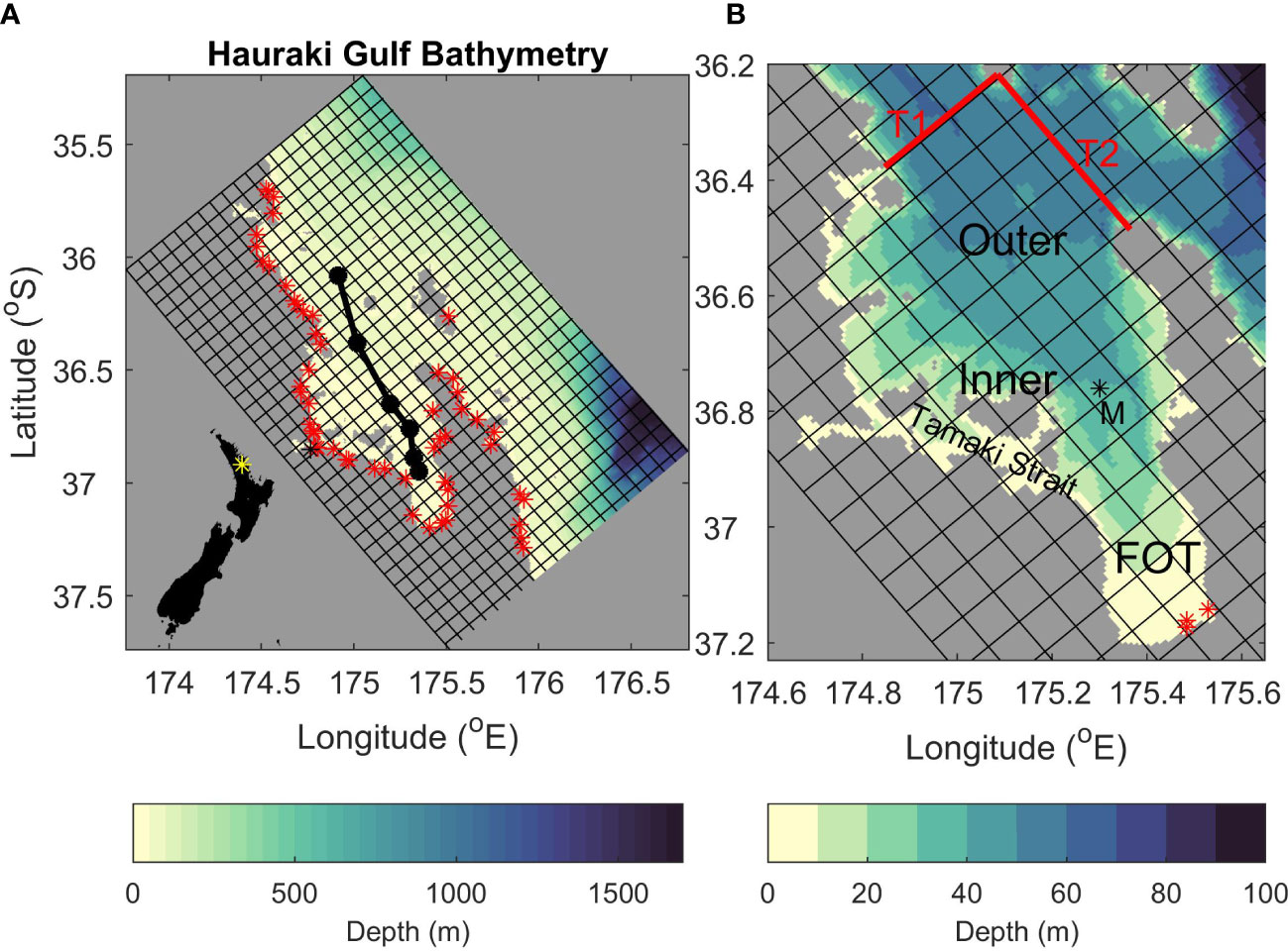
Figure 1 The model grid. Shading shows bathymetry and every 10th grid cell is indicated. (A) The full model grid with black dots indicating the position of CTD stations used in Figures 3–5. Red stars indicate the location of all rivers used in the time-averaged-river experiment. New Zealand’s capital city, Auckland is located at 36.8509° S, 174.7645° E and indicated by a black star. The insert in the bottom left indicates the study location as a yellow star on a map of New Zealand. (B) A zoom on the Hauraki Gulf. “M” indicates the position of the mooring data used in Figure 2. The red lines labelled “T1” and “T2” indicate the location of transects shown in Figure 9. “Inner”, “Outer” and “FOT” represent the inner Hauraki Gulf, the outer Hauraki Gulf, and the Firth of Thames respectively. Red stars indicate the locations of riverine inputs for the time-varying rivers experiment (The Waihou, Piako and Kaueranga Rivers from left to right).

In this work, we will investigate the effect of rivers upon the flows and primary productivity in the Hauraki Gulf and compare them with the cross-shelf exchanges of nutrients. This work builds on the available observational dataset through 1) providing higher spatial and temporal resolution and scenario testing that remove the effects of rivers and 2) comparisons of riverine versus offshore fluxes of nutrients. We discuss these results in terms of stressors in the region and the spatial distribution of risk from climate change versus risk from land use change. In doing this, we will address the following questions:

1. Are biogeochemical models suitable to study and understand stressors in this New Zealand deep-water estuary?

2. How do the rivers affect chlorophyll blooms in the Hauraki Gulf?

3. What is the extent and magnitude of riverine inputs and cross-shelf exchanges of nutrients?

Section 2 describes the model and experimental design. Section 3.1 compares the model to long-term observations. Biogeochemical observations in this region cover a long period of time but measurements are infrequent, so we also use the model to investigate how representative these observations are of seasonal processes. In Section 3.2 we investigate the footprint of the rivers using dye tracers, and in Section 3.3 we investigate how these rivers affect physical properties of the system. The effect of the rivers on biological production is investigated and compared to cross shelf exchanges of biological properties in Section 3.4 and 3.5. Section 3.6 investigates the variability of this system.

2 Materials and methods

2.1 Physical model setup

A regional ocean model (ROMS) (Shchepetkin and McWilliams, 2003; Shchepetkin and McWilliams, 2005) was set up with a resolution of 750 m for a region covering the Hauraki Gulf (Figure 1), and simulations were performed for the years 2004-2013. Boundary conditions were required for fluxes across the air-sea interface and lateral boundaries. Here the atmospheric forcing was timestamped and provided an ocean estimate for January 2004 to December 2013. Fluxes of heat and momentum between the atmosphere and ocean were calculated using data (6-hourly averages) from a global atmospheric reanalysis system, NCEP Reanalysis (Kalnay et al., 1996), with a heat flux correction term that nudged the model sea surface temperature (SST) towards observed SST (the NOAA Optimum Interpolation ¼° daily SST dataset, (Reynolds et al., 2007)). This heat flux correction term was given by

$$Q=\frac{dQ}{dsst}\ast (T_{model}-SST)$$

where dQ/dsst was set to 50 Watts m^-2°C^-1. The heat flux correction prevented the modelled SST from developing unnatural trends due to biases in the surface fluxes but had a negligible effect on day-to-day variability.

Lateral boundary conditions were specified for the barotropic and baroclinic velocity fields, the free surface, and tracers at the north, south, and east boundaries. The Shchepetkin and McWilliams (2005) condition was used for the barotropic velocity components, and the Chapman (1985) condition was applied to the free surface. These boundary conditions compare the barotropic velocities and sea level to externally defined boundary values and radiate the difference out of the model. In this model the externally defined boundary values were sourced from a 1/12° global HYCOM simulation (Chassignet et al., 2009). The boundary conditions for the baroclinic velocity field and the tracers were radiative with nudging to the HYCOM simulation at a time scale of 5 days. Tidal currents were added to the HYCOM velocities using amplitude and phase data for 13 tidal constituents (M2, S2, N2, K2, K1, 01, P1, Q1, 2N2, MU2, NU2, L2, T2) sourced from the NIWA New Zealand region tidal model (Walters et al., 2001). Coastal boundaries were specified via a land/sea mask. The western boundary was land.

2.2 Biogeochemical model setup

The Fennel biogeochemical model (Fennel et al., 2006) was used to provide state variable estimates for phytoplankton, ammonium (NH₄), nitrate (NO₃), zooplankton, large and small detritus and the equations that describe movement of nitrogen between these state variables. An additional chlorophyll variable accounted for chlorophyll stored in phytoplankton, which allowed for a variable chlorophyll to nitrogen ratio. Large and small detritus sunk at rates of 1 m d^-1 and 0.1 m d^-1, respectively.

Exchanges between the sediments and water column were accounted for via an assumption of instant remineralization of detritus when it sunk past the bottom of the lowest grid cell. Some (25%) of this detritus was released back into the water column as NH₄ with the remaining (75%) assumed to be removed from the system via denitrification. Data from other estuarine systems show that this assumption is a good one over long periods of time as most of the detrital matter that hits the seabed is eventually remineralized into the water column or lost as N₂ gas due to denitrification processes in the sediments (Fennel et al., 2006).

The biological model requires lateral boundary fluxes for all state variables and an incoming photosynthetically active radiation (PAR) across the ocean surface. The lateral boundary fluxes were sourced from a locally configured version of PISCES (Pelagic Interactions Scheme for Carbon and Ecosystem Studies; Aumont et al., 2015; see Supplementary Material 1 for a description of the model setup) which provides an estimate of the climatological annual cycle of biological variables. The PISCES model contains more state variables (e.g., two phytoplankton and zooplankton classes) than the Fennel model and the two PISCES phytoplankton (zooplankton) classes were combined to create a single phytoplankton (zooplankton) class to input into the Fennel model. PAR was imposed at the surface using estimates from NCEP Reanalysis (Kalnay et al., 1996).

2.3 Riverine inputs

The effect of rivers was included in the model as a point source in a grid cell adjacent to land, located near each river mouth. Incoming water (a volume flux of m³ s^-1), and nutrients (a concentration of mmol m^-3) were treated as a horizontal flow from the land into this grid cell. For this study we used two different estimates of the riverine inflows:

1) A climatological mean flow for all rivers sourced from the New Zealand river classification system (Booker and Woods, 2014; Whitehead and Booker, 2019)

2) Time varying flows for a few select rivers as described below.

Here the salinity of the incoming river water was set to zero and temperature was assumed to vary sinusoidally over the course of a year:

$$Temp=Tmean+Tamp\ast (\cos (day-daymax)\ast \frac{2\pi }{365})$$

where Temp is the temperature on a given date (day), daymax is the day of the maximum temperature, here set to day 45 (mid-February). The mean temperature (Tmean) was set to 15.6°C, a representative mean value for rivers in this region, sourced from the New Zealand River classification system (Booker and Woods, 2014; Whitehead and Booker, 2019). Tamp is the maximum temperature amplitude above the mean. Here Tamp was set to 4.02°C which gives a maximum temperature of 19.6°C, a typical summer maximum for river waters in this region.

Experiments forced with average river flows (shown in section 3.2) show that there are only a few rivers which dominate the response in this system and these rivers were chosen for time varying inputs. A combination of daily-average flow records and monthly water-quality sampling records from New Zealand’s National Rivers Water Quality Network (NRWQN) (Davies-Colley et al., 2011) were used to estimate annual nutrient loadings from the major rivers that flow into the Firth of Thames.

Data from 5 NRWQN stations were used:

1. Kaueranga River at Smiths cableway,

2. Ohinemuri River at Karangahake Gorge,

3. Waihou River at Te Aroha,

4. Waitoa River at Mellon Road and,

5. Piako River at Paeroa-Tahuna Road Bridge.

See Supplementary Material 2 for location of these stations. These monthly water quality and daily water flow data were converted into estimates of the daily loads of NO₃, NH₄ and total nitrogen (TN) by fitting the data to a model of riverine flow using the USGS LOADEST method (Runkel et al., 2004). The portion of total nitrogen not accounted for by NO₃ and NH₄ was allocated to the large detrital field for input into the model (i.e., large detritus = TN-NH₄-NO₃).

The Ohinemuri River feeds into the Waihou River and the Waitoa River feeds into the Piako River so the contributions from these rivers were joined for inputting into the model. This meant that there were three rivers flowing into the ocean modelling domain: the Waihou, Piako and Kaueranga Rivers (indicated on Figure 1B).

The NRWQN data station on the Kaueranga River is near the river mouth and the river flow and nutrient estimates calculated above were used for this river. The NRWQN stations used for river flow and nutrient estimates for the Waihou and Piako were located 10s of kilometers upstream of the river mouths and a scaling factor was used to account for changes in water properties between the upstream measurements and the river mouth where the water flows into the model domain. To calculate the scaling factor for the river flow between upstream and the river mouth, the New Zealand river classification system data (Whitehead and Booker, 2019; Whitehead, 2019) were used to get an annual average of river flows at the upstream NRWQN stations and at the river mouths. These numbers were used to calculate an average ratio between flows at the NRWQN measurement sites and at the river mouth (Table 1). The time-varying flows calculated for the upstream NRWQN measurement sites at Waihou and Piako were scaled by 1.211 and 2.670 respectively to estimate the flows at the river mouth. The scaling factor for nutrients was estimated from Zeldis et al. (2015). They calculated that total estimates of total nitrogen load from the upstream NRWQN measurement sites should be increased by a factor of 1.92 to get an estimate of total nitrate load (kg y^-1) at the river mouths. When accounting for the increase in total nitrogen already accounted for due to the above calculated scaled increase in river volumes (and associated increase in total nitrogen), this yielded a scaling factor of 1.585 and 0.72 to be applied to each of the nutrient concentrations (NH₄, NO₃ and large detritus) for the Waihou and Piako rivers respectively.

TABLE 1

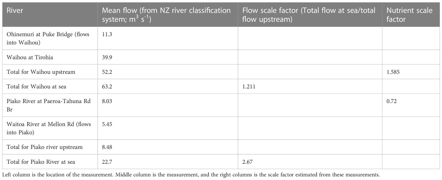
Table 1 Scaling factors for the rivers.

2.4 Model experiments

Four different experiments were performed using this model. The first (time-averaged-river) used only the physical model with a constant time-averaged flow for each of the rivers in the Hauraki Gulf. The water coming in from each of these rivers was marked with a passive tracer (“dye”) of concentration 1 kg m^-3. This passive tracer was moved around the model following the same numerical schemes as the temperature, salinity and biological tracers and was used to indicate the concentration of riverine water in each model grid cell. The second experiment (no-river) was the same setup except with no riverine inputs. The third experiment (time-varying-river) used the full coupled physical-biogeochemical model to investigate the effects of nutrient inputs from the rivers into the Hauraki Gulf, with the time-varying water flow and nutrient concentrations described in the previous section. A fourth experiment (time-varying-nobio) was performed using the same biogeochemical model and time-varying riverine flows as the third experiment, but riverine nutrient and detrital inputs were set to zero. The difference between the third and fourth experiments were examined to elucidate the effect of the riverine inputs of nutrients to the region.

2.5 Data processing

Timeseries of temperature and salinity were collected at depths of 7, 10, 20 and 33 m for temperature and 10 and 34 m for salinity at a mooring located in the Firth of Thames (see Figure 1B for location; Zeldis and Swaney, 2018).

Seasonal biogeochemical data for NO₃, NH₄ and chlorophyll were collected using discrete rosette samples from CTD casts along a transect (indicated in Figure 1A) from intermittent (1-4 times per year) surveys between 1996 and 2013. There were 6 stations along the transect (see Figure 1 for location) and samples were taken at approximately 5-10 m depth-intervals. All data were interpolated vertically to common depths of 1 m intervals. In addition to these, biogeochemical data for NO₃, NH₄ and chlorophyll were taken using discrete rosette samples from CTD casts at the mooring location when the (above mentioned) mooring was serviced. See Zeldis et al. (2022) and Zeldis and Swaney (2018) for more information on the data used here.

Following Zeldis and Swaney (2018), these two biogeochemical data sets were collated into a gridded seasonal climatology of NH₄, NO₃ and chlorophyll. To calculate these climatologies, the average of all data collected during each season (summer, autumn, winter, and spring) was calculated at each station and at each 1 m interpolated depth-bin. The resultant pooled dataset contains 45 surveys with 5 in summer, 16 in autumn, 9 in winter and 15 in spring. These datapoints were not spread evenly throughout the season with more observations concentrated in the start of summer and autumn and more observations concentrated in the middle of spring and winter (Table 2). Additionally, not every station was sampled during each field survey and the number of observational points for each station is indicated at the top of the figures referenced in Section 3.1.2

TABLE 2

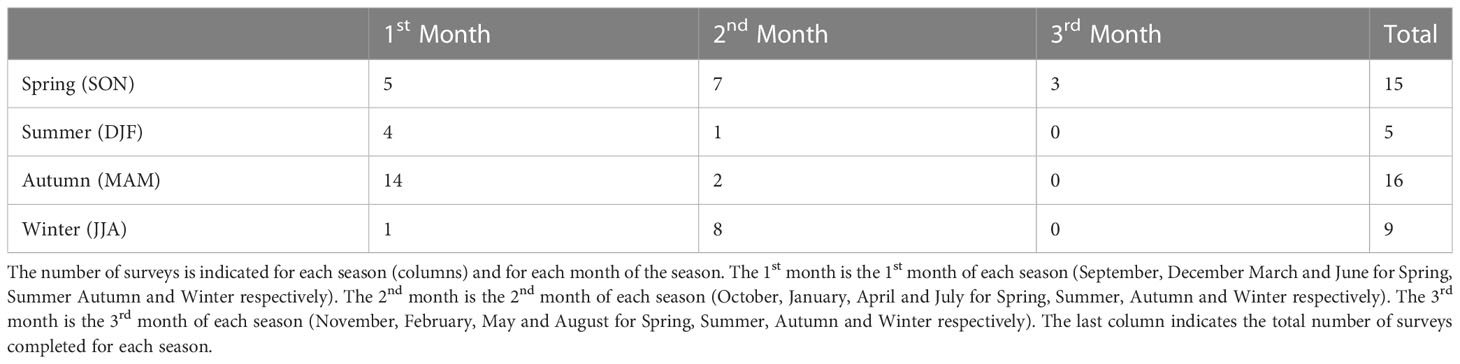
Table 2 Number of field surveys which collected data along the transect (location of transect indicated in Figure 1A).

For the model/data comparisons shown in section 3.1, two modelled seasonal climatologies were calculated. The first climatology is a like-for-like comparison where modelled output was sampled at the same time of year and positions as the data, and a climatology was calculated using the same processes used for calculating the observed climatology (like the climatologies presented in Zeldis and Swaney (2018) and as described above).

There are two issues which create some uncertainties with a modelled or observed climatology calculated using this sampling regime:

1) the small sample size and discreate temporal and spatial sampling means that the climatology can be biased if the comparatively sparse sampling has inadequately sampled the true, long-term distribution of ocean weather patterns and,

2) the climatology can be biased by sample collection which is focused on one end of the season.

For example, a climatological average of summer conditions calculated using the data shown in Table 2 will be more representative of the oceanic conditions at the start of summer than the middle or end. To estimate the effect of these issues on the climatology inferred from the field-data, a second modelled climatology was created to compare to the first modelled climatology. The second climatology is the true modelled seasonal climatology. This climatology was calculated along the same transect as the observations but at the higher resolution of the model (750 m) and not subsampled in time or space so that this calculated climatology was unbiased by the sampling regime. This gave us three climatologies which we compared:

1) an observed climatology (similar to Zeldis and Swaney (2018)),

2) a subsampled modelled climatology (the modelled version of the Zeldis and Swaney (2018) climatologies) and,

3) a full model climatology that represented the true modelled estimate of the climatology.

When the 2nd and 3rd climatologies agreed this indicated that the subsampling methods were not introducing biases into the observed climatology. When the 1st, 2nd, and 3rd climatologies agreed this indicated a good model/data comparison. When the 2nd and 3rd agreed but did not agree with the 1st this indicated the subsampling methods were not introducing biases, but the model was unable to replicate the observations. When the 2nd and 3rd climatologies did not agree this indicated insufficient knowledge to perform the model/data assessment; either there were biases introduced by the observational sampling method, or the model had more variability and extreme events than the observations.

2.6 Model and data comparisons

To formally compare model climatologies and time-series with data, two statistics were calculated: a bias and an unbiased root mean squared error (RMSE). The bias and RMSE are given by (Jolliff et al., 2009):

$$\begin{array}{c}Bias=\frac{1}{n}{\displaystyle {\sum }_{n}M-O}\\ RMSE=(\frac{1}{n}{\displaystyle {\sum }_n{(\left(M-\overline{M}\right)-\left(O-\overline{O}\right))}^2{)}^{0.5}}\end{array}$$

where M is the model and O is the observations, n is the number of observations and overbars represent averages. In Section 3.1.2, there were comparisons between the two modelled climatologies (as described above) and in this case O represents the full model and M represents the subsampled model. All modelled datasets were linearly interpolated in time and space and/or subsampled onto the observational data locations. This included the comparisons of the full model output with the subsetted and/or observations and it should be noted that for these statistics we were only comparing the difference created with temporal (not spatial) subsampling.

Variance (Var) and range was calculated for observational datasets and used as a comparator to the above statistics. These were calculated as such:

$$Var=\frac{1}{n}{\displaystyle {\sum }_n(O-\overline{O}})$$

$$Range=\max (O)-\text{min}(O)$$

where O is the observations, n is the number of observations and overbars represent averages.

3 Results

3.1 Model and data comparisons

3.1.1 Physics

The observed temperature has a seasonal cycle with maxima of approximately 22°C during summer/autumn months and minima of approximately 11°C during winter/spring months (Figures 2A–D). Superimposed onto this seasonal cycle, there are some minor temperature variations (approximately +/- 1-2°C) at sub-seasonal scales (Figure 2). The modelled temperature for the different scenarios (time-varying-river, time-averaged-river, and no-river) has a similar seasonal cycle to the observations and the temperature closely matches the observed temperature at all depths (RMSE<1.2°C; Table 3), with an underestimation of temperature of up to 2°C in winter/spring. This underestimation is present throughout the water column, suggesting that it arises from heat fluxes from the atmospheric or lateral boundary conditions. There is no persistent bias in summer. The modelled scenarios all also produce small sub-seasonal scale variability such as those seen in the observations (approximately +/- 1-2°C). Temperature variations are strongly modified by atmospheric fluxes, the offshore boundary conditions and vertical mixing and the good agreement between the observed and modelled temperatures indicate that the model is capturing these processes except for the above-mentioned bias in heat fluxes during winter/spring. The differences in temperature between the different model scenarios (which change the riverine inputs) are small in comparison with seasonal scale fluctuations, indicating that the input of riverine water does not have a large effect on modelled temperature.

FIGURE 2

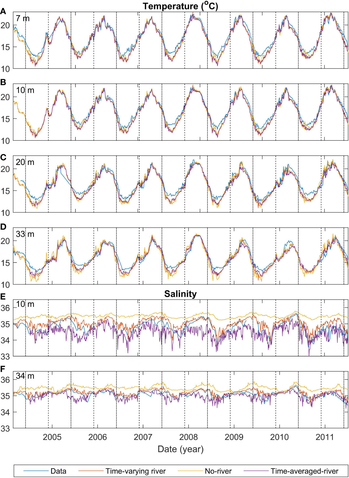
Figure 2 Comparisons of time series of model and observed temperature at the mooring for depths of 7 m (A), 10 m (B), 20 m (C) and 33 m (D), and salinity for depths of 10 m (E) and 34 m (F). Blue lines indicate the observed temperature, red, orange and purple lines indicate different model runs (time-varying-river, no-river and time-averaged-river respectively). Black dashed (dashed-dotted) lines indicate the start of summer (winter). The time-varying-nobio has the same physical inputs as the time-varying-river and thus is not shown in this figure.

All scenarios have a seasonal variation in salinity that is created from seasonal-scale fluctuations in local evaporation/rainfall and offshore conditions (Figures 2E, F). However, salinity is more strongly affected by riverine inputs, and variability in the strength and positioning of the riverine plume (see Section 3.5.1) creates greater daily to weekly observed salinity variability than the temperature (Figures 2A-D). The model is not expected to capture this small-scale variability, and this leads to high RMSE compared to the variance for salinity (RMSE 0.21 -0.44 g kg^-1 compared with variance of 0.21-0.41 g kg^-1). There is a notable difference between the model scenarios with the time-averaged-river scenario producing the lowest salinity waters, the time-varying-river scenario producing the next lowest and the no-river scenario producing salinities that are higher than the other two scenarios. The riverine input does have a clear effect on the salinity in the model domain, with the riverine input scenarios producing smaller magnitude biases (<0.29 g kg^-1 compared with<0.74 g kg^-1) than the no-river scenario (Table 3). For the rest of this section, we only describe the two scenarios which have an input of riverine water (time-varying-river and time-averaged-river).

TABLE 3

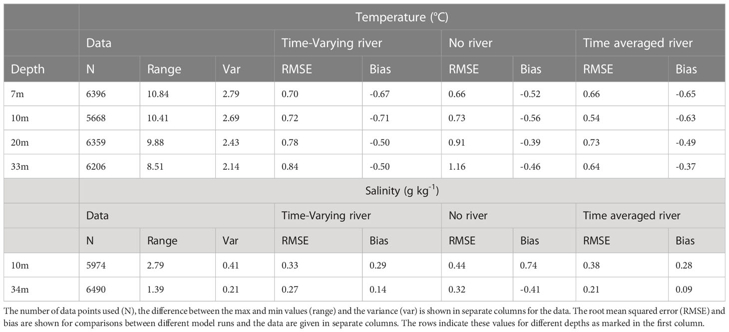
Table 3 Statistics for the time series comparisons presented (see also Figure 2).

Similar to temperature, the two riverine scenarios (time-averaged-river and time-varying-river) capture the seasonal variability of salinity with peaks and troughs occurring at similar times as the observed. The modelled salinity peaks at 35.4 g kg^-1 and 35.5 g kg^-1 and has a minimum of 33.2 g kg^-1 and 33.5 g kg^-1 for the time-averaged-river and time-varying-river scenarios respectively. The observed salinity has a maximum of 35.5 g kg^-1 and a minimum of 33.5 g kg^-1. In general, the modelled salinities in the time-varying-river scenario are slightly greater than observed and the time-average-river scenario gives slightly lower salinities than observed. The good agreement between modelled and observed salinity indicates that the modelled riverine inputs are capturing the volume of water coming in from the rivers and its subsequent transport into the vicinity of the monitoring buoy in the northern Firth of Thames.

3.1.2 Biology

The observed summer NO₃ is high (>6 mmol m^-3) in offshore and deeper (>50 m) regions (Figure 3A). This is not replicated in the modelled subsampled climatology, which tends to have lower NO₃ (<4 mmol m^-3 resulting in a bias of -1.93 mmol m^-3; Table 4) and homogeneous concentrations throughout the water column and along the transect (Figure 3E). The full modelled climatology, however, does replicate an increased NO₃ at depths offshore, albeit at a lower concentration than observed (~5-6 mmol m^-3, resulting in a smaller bias of -1.7 mmol m^-3 Figure 3I and Table 4). The observed summer NO₃ has a large variance (4.54 mmol m^-3) which means that a small sample size such as the one we are using here is less able to represent the summer NO₃ and this is reflected in the larger differences when comparing the full and subsampled climatologies (RMSE=2.34; Table 4) and will also contribute to the large RMSE for each of the modelled climatologies (RMSE of 1.96 mmol m^-3 and 3.1 mmol m^-3 for the full and subsamples climatologies respectively).

FIGURE 3

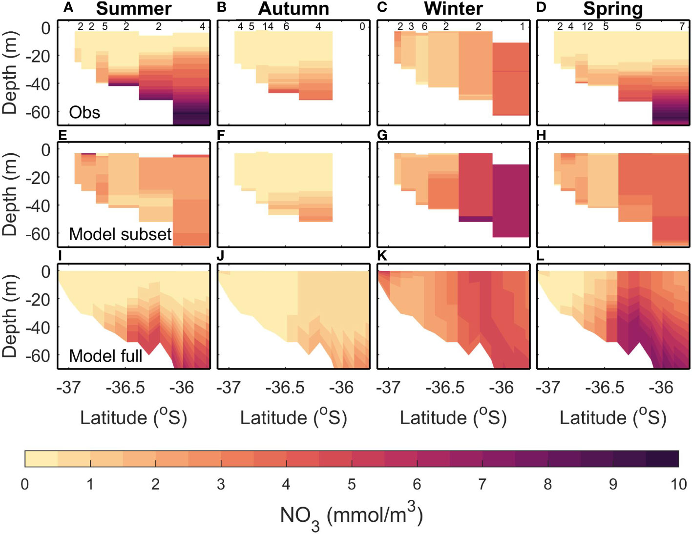
Figure 3 Comparisons of climatological modelled and observed NO₃ for a transect extending from the Firth of Thames to the outer Hauraki Gulf. Each column shows a different season: Summer (DJF; A, E, I), Autumn (MAM; B, F, J), Winter (JJA; C, G, K), Spring (SON; D, H, L) (from left to right). Top row (A–D) shows an observed climatology calculated from repeated data collection along this transect. Middle row (E-H) shows a modelled climatology calculated by subsampling the time-varying-river scenario in time and space in a similar fashion to the observed data. Bottom row (I-L) shows the modelled climatology without temporal subsampling (i.e., using all model outputs in the time-varying-river scenario). There are six stations sampled, and the number of samples taken at each station is indicated in black at the top. See Table 2 for more details.

TABLE 4

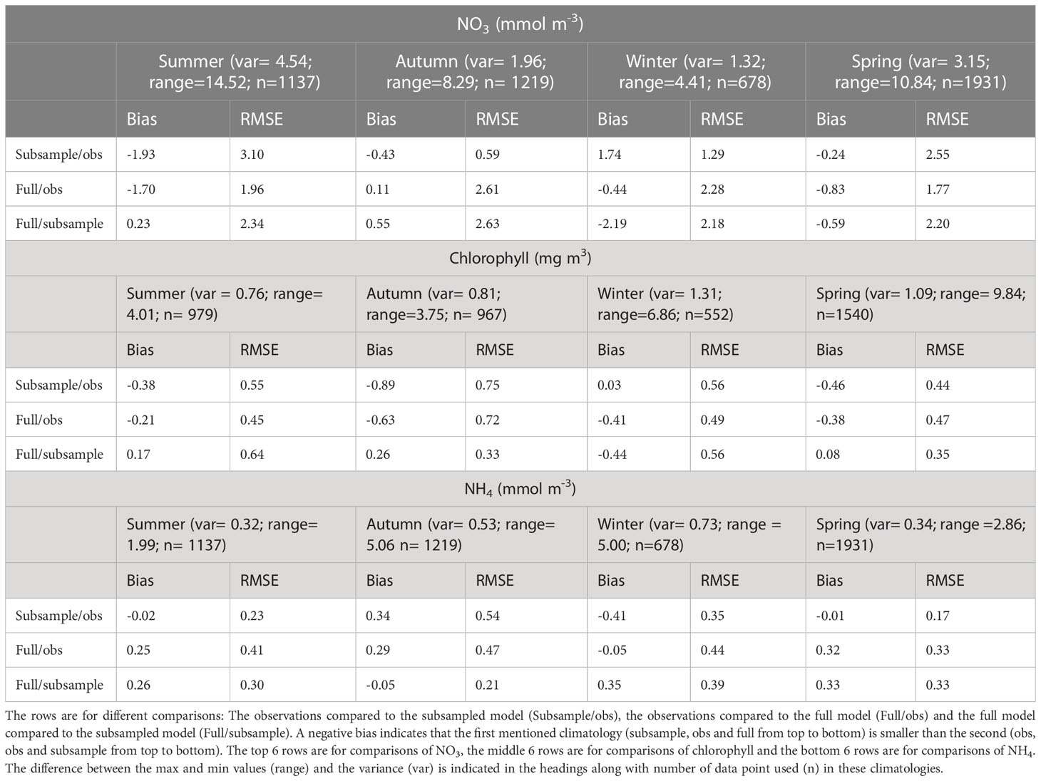
Table 4 The rows show the bias and the unbiased root mean squared error (RMSE) between observation and modelled climatologies for each of the seasons (Summer, Autumn, Winter, Spring).

In autumn, observed surface waters are depleted of NO₃ (<0.5 mmol m^-3) but there is an increase (to 1.5-3 mmol m^-3) at depths below 30 m (Figure 3B). Both the modelled full (Figure 3F) and subsampled climatologies (Figure 3J) replicate the depleted surface NO₃ and increased NO₃ in the subsurface. For both the models compared to the observations, the RMSE is less than the 2.63 mmol m^-3 error introduced by subsampling (i.e., the comparison between the two modelled climatologies) and the bias magnitude is less than 0.43 mmol m^-3 (Table 4).

In winter, the observed NO₃ has a cross-shelf gradient ranging from a low of<0.5 mmol m^-3 in the shallower regions and increasing to 4-5 mmol m^-3 in the deeper regions (Figure 3C). This increase of nutrients in the deeper regions is due to low light levels limiting phytoplankton growth (Zeldis et al., 2022). Both the subsampled (Figure 3G) and full model climatologies (Figure 3K) replicate this gradient, although in general the NO₃ is slightly higher in the subsampled model than observed (ranging from 1 mmol m^-3 to 7.5 mmol m^-3). The variability in this time period is low (1.32 mmol m^-3), but the RMSE between the full and subsampled models is high in comparison (2.18 mmol m^-3) which indicates a potential for errors in the sampling regime and we are unable to determine if the modelled bias and RMSE are due to errors in the model or sampling regime.

In spring, the observed climatology shows NO₃ depletion in shallow depths and surface waters but high NO₃ (>2 mmol m^-3) concentrations at depths greater than 30 m (Figure 3D). The subsampled model climatology does not replicate the observations, with NO₃ being well mixed throughout the water column (Figure 3H). The full climatology does replicate the along-transect gradient of NO₃ (low values inshore and high values offshore) however, the NO₃ is still well mixed throughout the water column in the offshore regions (Figure 3L). There is a high variability seen in the observations (3.15 mmol m^-3; Table 4) which is then reflected in a high RMSE between the full and subsampled climatologies (2.20 mmol m^-3). This variability and uncertainties introduced by the sampling errors is reflected in higher RMSE for the model/data comparisons (2.55 mmol m^-3 and 1.77 mmol m^-3 for the subsampled and full climatology respectively). Whilst these RMSE are less than the variability, it should be noted that the model is performing poorly in the surface but a good comparison at depth brings down the overall RMSE.

The largest concentrations of chlorophyll in the Hauraki Gulf tend to occur near the rivers at the southern end of the Firth of Thames, grown from riverine inputs of nutrients (located on the southern end of the transects in Figures 3–5). Observed summer chlorophyll indicates a subsurface maximum which is most pronounced near the river mouth but present throughout the Hauraki Gulf (Figure 4A). The modelled subsampled climatology creates a summer surface chlorophyll maximum near the river mouth but does not have the subsurface maximum in the outer Hauraki Gulf (Figure 4E). However, the modelled full climatology replicates the subsurface chlorophyll maximum (Figure 4I), indicating that the model is creating this bloom at different times to when it is measured. This variability in the timing of the chlorophyll bloom is seen in the RMSE between subsampled and full model climatologies (0.64 mg m^-3; Table 4) which is comparable to the variance (0.76 mg m^-3). The RMSE in the model/data comparisons are comparable but slightly smaller (0.55 mg m^-3 and 0.45 mg m^-3 for the subsampled and full climatologies respectively).

FIGURE 4

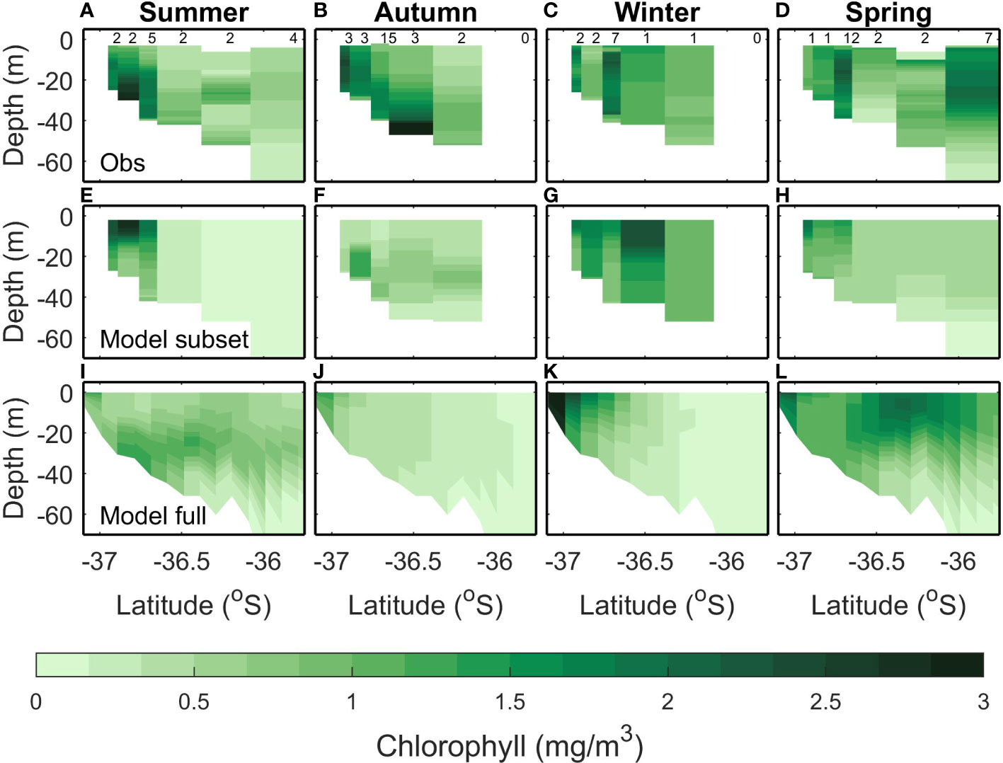
Figure 4 Same as Figure 3 but for Chlorophyll.

In autumn, the observed climatology has increased chlorophyll concentration near the rivers and a bottom chlorophyll bloom at -36.5°S (Figure 4B). A mid water column chlorophyll bloom is present in the modelled subsampled (Figure 4F) climatology and the full climatology produces a higher (apparent) chlorophyll concentration near the river mouth (Figure 4J). However, in both modelled climatologies, the concentrations are lower than the observed (<1 mg m³ for modelled compared to up to 3 mg m^-3 for the observed). This is reflected in the bias (-0.63 mg m^-3 and -0.89 mg m^-3) and RMSE (0.72 mg m^-3 and 0.75 mg m^-3) that are comparable to the observed variance (0.81 mg m^-3) for both the full and subsampled model climatologies. The bias magnitude and RMSE are small for the comparison between the two model climatologies (0.26 mg m^-3 and 0.33 mg m^-3 respectively) which suggests that the larger bias magnitude and RMSE between the model and observed climatologies are due to the model not capturing the near bottom chlorophyll dynamics in autumn.

In winter, the observed chlorophyll concentrations are in the range 0.5-2 mg m^-3 with peaks occurring at the river mouth and the middle of the transect (Figure 4C). The modelled subsampled winter chlorophyll has a similar range, with peaks also occurring near the river mouth and in the middle of the transect (Figure 4G). The modelled full climatology, however, has lower concentrations (<0.5 mg m^-3) offshore and only reproduces the chlorophyll peak at the river mouth (Figure 4K). The RMSE (<0.56 mg m^-3) and bias magnitude (<0.44 mg m^-3) are low compared to the variability (1.31 mg m^-3 for all comparisons; Table 4).

In spring, the observed chlorophyll concentrations are raised across the whole transect (Figure 4D). This is not replicated in the subsampled climatology (Figure 4H), which only has an increase in chlorophyll near the river mouth, however, the full climatology replicates the increased chlorophyll concentrations across the transect (Figure 4L). That the model captured this in the full but not the subsampled climatology suggests that there is some variability in the initialization of the spring bloom. This is reflected in the statistics where the RMSE (≤0.47 mg m^-3) and bias magnitude (≤0.46 mg m^-3) are low for all climatological comparisons when compared to the variability (1.09 mg m^-3; Table 4).

Observed summer NH₄ is patchy, with a slight increase towards the lower layers (Figure 5A). The subsampled model climatology is similar, with a larger increase towards the lower layers (Figure 5E). The full model climatology also shows a bottom maximum in NH₄ (Figure 5I). However, the modelled bottom NH₄ maximum is larger than observed, resulting in a large bias magnitude (0.41 mmol m^-3) for the full climatology. This large bias magnitude and large RMSE for the full climatology can be explained by the high RMSE (0.30 mmol m^-3) between the full and subsampled climatology. However, the subsampled climatology has small bias (-0.02 mmol m^-3) and RMSE (0.23 mmol m^-3).

FIGURE 5

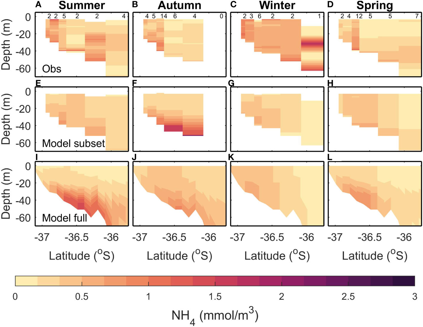
Figure 5 Same as Figure 3 but for NH₄.

In autumn, the observed climatology (Figure 5B) has a full water column increase in NH₄ near the river mouth, with values decreasing offshore, whereas both the modelled climatologies (Figures 5F, J) have a bottom NH₄ maximum that is not seen in the observed. The RMSE (≤0.47 mmol m^-3) and bias magnitude (≤0.29 mmol m^-3) are low compared to the variability (0.53 mmol m^-3) for the full versus subsampled and full versus observation comparisons (Table 4). The subsampled versus observed has an RMSE which is higher than the variability (0.54 mmol m^-3).

In winter, the observed NH₄ is fairly homogeneous (values approx. 0.5 mmol m^-3) except for the deepest profile which has lower NH₄ in the mid-water column and near the bottom (Figure 5C). Both the modelled climatologies have lower NH₄ than the observed, and there is a more pronounced gradient between the higher inshore values and lower offshore values (Figures 5G, K). However, the bias magnitude (≤0.41 mmol m^-3) and RMSE (≤0.44 mmol m^-3) are small when compared to the variability (0.73 mmol m^-3) for all 3 comparisons.

In spring, the observed NH₄ has increased values inshore, and at depth<40 m offshore (Figure 5D). Both the modelled climatologies replicate this (Figures 5H, L), although the inshore maximum tends to be bottom intensified in the modelled climatologies and the modelled climatologies tend to be homogeneous throughout the water column in the observed. The RMSE between the full and subsampled modelled climatology (0.33 mmol m^-3) is close to the variability (0.34 mmol m^-3) which indicates that the sampling regime may be inadequate in capturing the true climatology. This is reflected in the higher RMSE (0.33 mmol m^-3) and bias magnitude (0.32 mmol m^-3) for the full modelled climatology compared to observations, although the subsampled model performs well compared to observations with small RMSE and bias (0.17 mmol m^-3 and -0.01 mmol m^-3 respectively).

3.2 The footprint of the rivers

Dye tracers (unique to each river) were released at the modelled river entrances to indicate the footprint of the rivers in the time-averaged-river scenario (Figure 6). The dye was released at a concentration of 1kg m^-3 so that a dye concentration of 1kg m^-3 indicates that the water mass was 100% riverine water and a dye concentration of 0 means that 0% of the water mass was riverine water. The largest riverine flows into the modelling domain come from three rivers at the bottom of the Firth of Thames (indicated in Figure 1B). Hence, we show the dye tracers released from these rivers combined in Figure 6A and the remaining rivers combined in Figure 6B. Here we focus on the surface dye concentration, but the results are similar for subsurface dye concentrations (see Supplementary Material 3). The dye concentration in the whole Hauraki Gulf region is dominated by the dye released from the three main rivers at the bottom of the Firth of Thames. The other rivers combined have a small footprint in the Tamaki Strait at the south-eastern part of the domain (longitude 174.6° E to 175.2 °E and latitude 36.8 °S to 36.9 °S; see Figure 1 for location). However, the concentration of the dye in the Tamaki Strait that originated locally is still smaller than the dye concentration that originated non-locally from the three main rivers. For the rest of the Hauraki Gulf, inputs of nutrients from the minor rivers have a very localized effect at some river mouths.

FIGURE 6

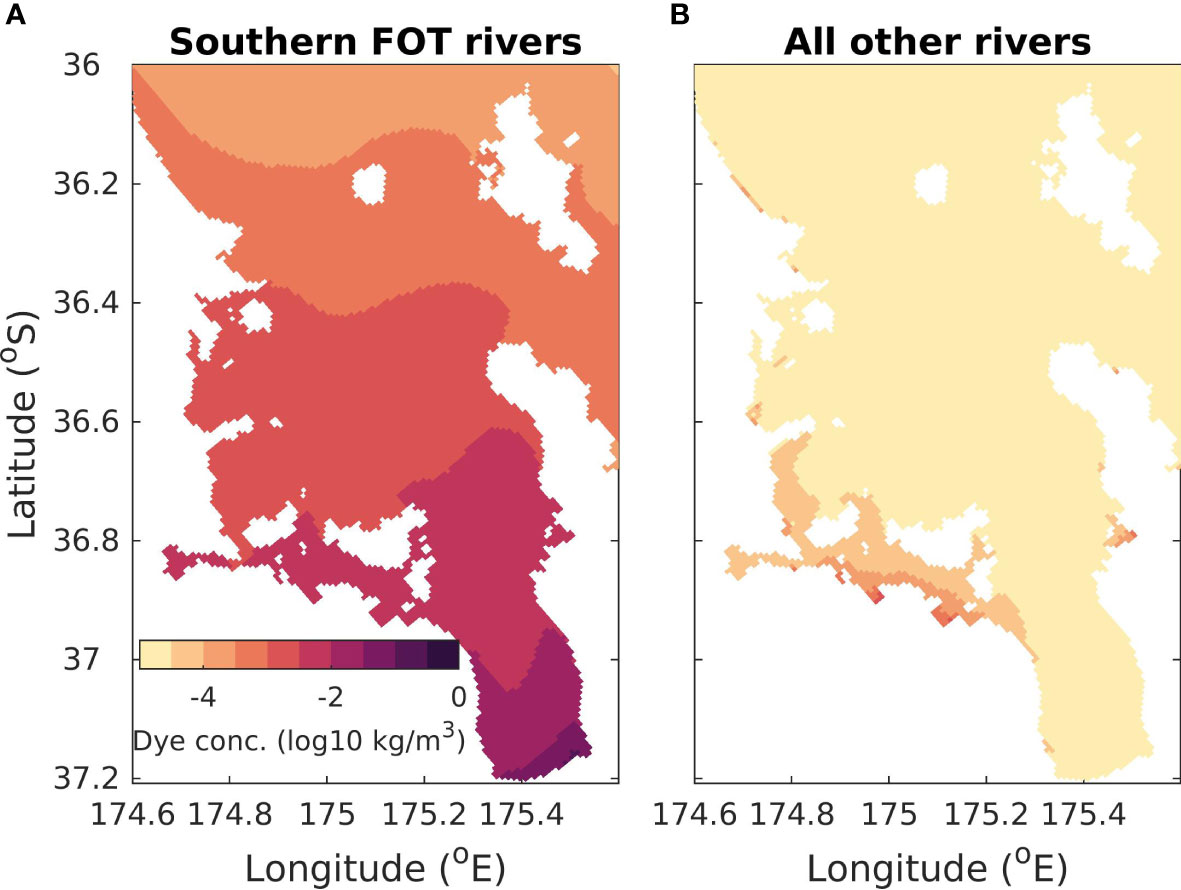
Figure 6 Average surface concentration of dye released from rivers at a concentration of 1kg m^-3 in the time-average scenario. (A) The contribution to dye concentration from three rivers located at the bottom of the Firth of Thames (see Figure 1B for location). These are the rivers used in the time-varying-river and time-varying-nobio scenarios. (B) The contribution from all other rivers in this domain. Note that color is on a log-scale.

The highest concentrations of riverine water (Figure 6A) occur near the mouths of the three rivers in the Firth of Thames. The concentration of riverine waters decreases away from the river mouths, with less than 0.001% of the waters in the outer Hauraki Gulf coming from riverine inputs. As the Firth of Thames rivers dominate this system, in subsequent sections we focus on the scenarios with time varying river inputs from the 3 main rivers in the Firth of Thames.

3.3 The effect of riverine input on physical processes

Changes in the riverine inputs can alter the salinity, density, and subsequent flows of the Hauraki Gulf region (as seen in the difference in the time-varying-river and no-river scenarios; Figure 7). The areas with the largest riverine concentration are in the Firth of Thames and this is the region which has some of the largest changes when riverine inputs are removed from the model. The biggest differences between the two simulations (time-varying-river and no-river scenarios) are seen in the modelled salinity (Figures 7A–C). The riverine inputs are associated with a lowering of the salinity and when riverine inputs are activated a low salinity plume is evident in the time-averaged surface modelled fields on the eastern side of the Firth of Thames. A lowered salinity value reaches into the outer Firth of Thames with salinity differences evident as far north as 36.6°S.

FIGURE 7

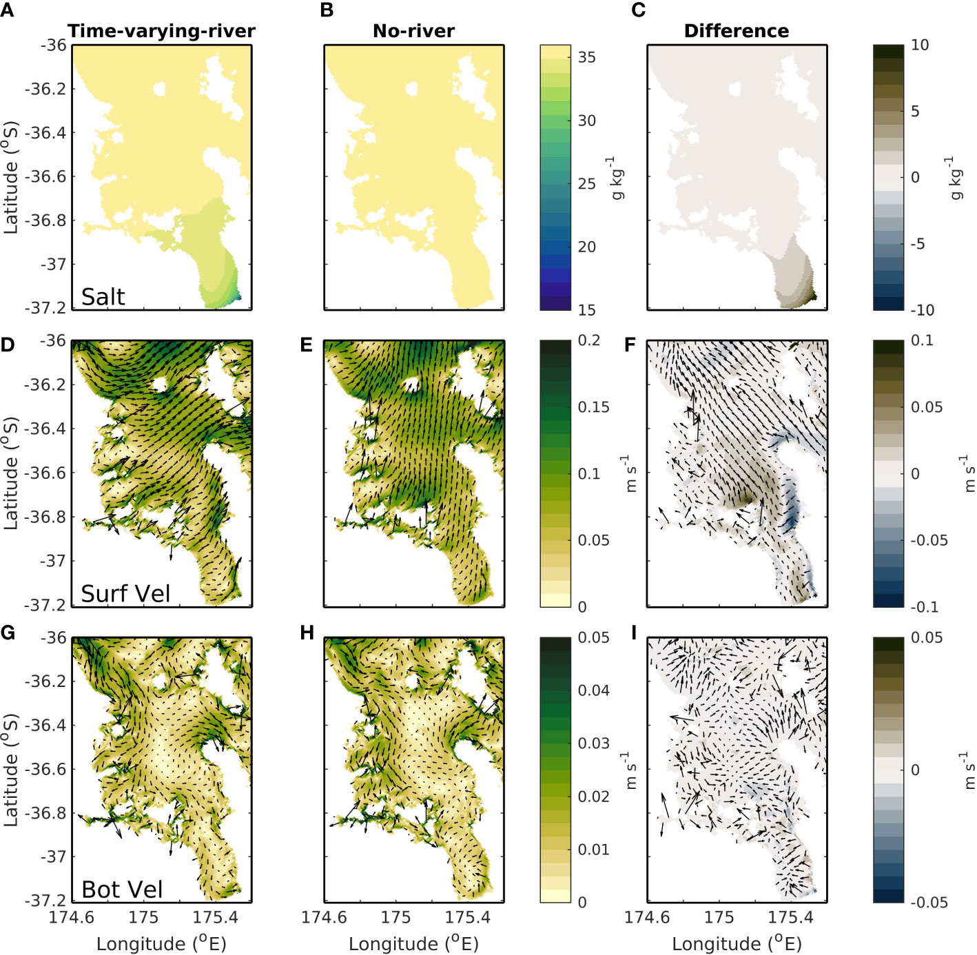
Figure 7 Top row (A–C) shows average surface salinity, middle row (D–F) shows average surface current speed and bottom row (G–I) shows average bottom current speed. Left column (A, D, G) is for a simulation with riverine inputs (the time-varying-river scenario), middle column (B, E, H) is for a simulation with no riverine inputs (the no-river scenario) and right column (C, F, I) is the difference between these two simulations.

The oceanic flows are also impacted by the flow of low-salinity water into the domain (Figures 7D–I). When riverine inputs are present, there is a northward surface current of<0.1 m s^-1 associated with the riverine plume (Figure 7F). On average this current is situated to the eastern end of the Firth of Thames and carries riverine water up to the entrance of the Hauraki Gulf. The riverine waters are near the surface of the water column, and the associated current is strongest at the surface and becomes weaker with depth. In the near bottom this current is almost negligible with difference in velocities between the time-varying-river and no-river scenarios of less than 0.005 m s^-1 (Figure 7I).

3.4 The effect of riverine input on biological processes

Rivers are a large source of nutrients to the system and in the time-varying-river scenario there is a large plume evident in the Firth of Thames associated with the input of nutrients from the rivers (Figure 8A). In comparison, the nutrient concentrations in the Firth of Thames are low for the time-varying-nobio scenario (Figure 8B), indicating that the source of nutrients in the Firth of Thames is mostly from riverine input; the non-riverine sources of nutrients (offshore cross-shelf exchange) do not extend this far into the Hauraki Gulf. As such, the difference between the time-varying-river and time-varying-nobio scenarios are greater in the Firth of Thames, reaching values of up to 10 mmol m^-3 (Figure 8C). Further north, the nutrient concentration in the time-varying-river scenario is small compared to the concentrations in the Firth of Thames. The time-varying-nobio scenario also has a similar nutrient concentration and the difference between the time-varying-river and time-varying-nobio scenarios is small in the outer Hauraki Gulf (<0.1 mmol m^-3). This indicates that the nutrient supply in the outer Hauraki Gulf is not sourced from the rivers but is dominated by other processes such as the offshore exchanges of nutrients.

FIGURE 8

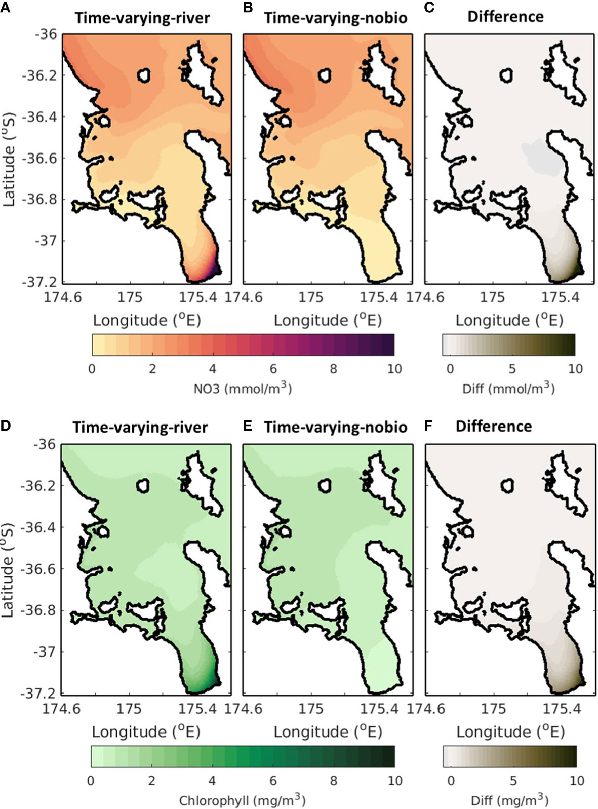
Figure 8 Time-averaged surface NO₃ (top; A–C) and chlorophyll (bottom; D–F). Left (A, D) is for the time-varying-river scenario, middle (B, E) is for the time-varying-nobio scenario and right (C, F) is the difference between these. A positive (negative) value in the right panel indicates that the time-varying-nobio (middle) simulation has a smaller (larger) concentration however values are always positive as the time-varying-river simulation always has chlorophyll and NO₃.

The results are similar for chlorophyll. The input of nutrients from the rivers creates a phytoplankton bloom and, in the time-varying-river simulation, there is a phytoplankton plume that forms at the river mouth (from riverine inputs of nutrients) and extends into the Firth of Thames. At the river mouth, the difference between the time-varying-river and time-varying-nobio scenarios reaches a peak (>10 mg m^-3). Outside of the Firth of Thames, chlorophyll concentrations derived from riverine sources of nutrients are small as other processes dominate and the difference between the time-varying-river and the time-varying-nobio scenarios decreases to a minimum (<0.1 mg m^-3) in the outer Hauraki Gulf.

Near bottom NO₃ and chlorophyll concentrations for the time-varying-river and time-varying-nobio scenarios are shown in Supplementary Material 4. Slower currents on the bottom, the lack of a river-induced flow (see Figures 7F, I) and mainly surface nutrient inputs from the rivers mean that the difference between the time-varying-river and time-varying-nobio scenarios is more noticeable at the surface.

3.5 Nutrient budgets

Modelled fluxes of nitrogen in and out of the Hauraki Gulf region occur due to riverine inputs, fluxes at the oceanic boundary and a denitrification flux caused by processes occurring in the sediments (Figure 9). On average, there is a flow in the time-varying-river scenario into the Hauraki Gulf through transect 1 (Figure 9A; location marked as T1 on Figure 1B), creating a flux of nitrogen into the Hauraki Gulf. At the surface, this tends to flow zonally, across the top of the Hauraki Gulf (see Figure 7), which results in a flux out of the domain in the surface of transect 2 (Figure 9B; location marked as T2 on Figure 1B). The subsurface flows in this region are weaker but flow through transect 1 into the Hauraki Gulf with subsequent flow out via transect 2 (Figure 9B). However, the resulting flux out of transect 2 is less than that which comes in via transect 1 (Figure 9B).

FIGURE 9

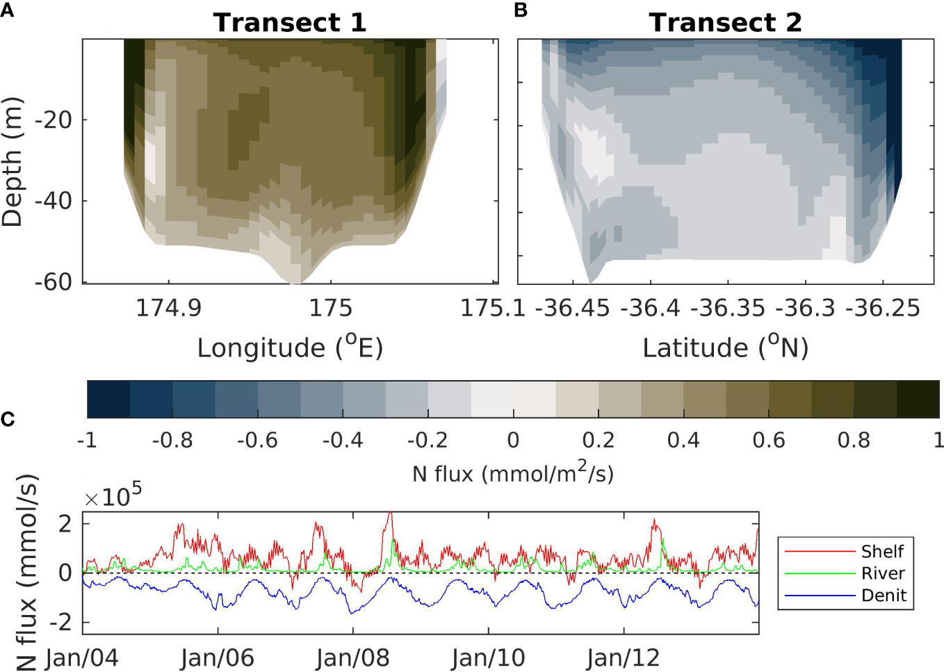
Figure 9 Total nitrogen flux calculated as the sum of nitrogen stored in each of the model classes (NO₃, NH₄, phytoplankton, zooplankton and detritus). Top left (A) shows fluxes over the northern continental shelf boundary to Hauraki Gulf. Top right (B) shows fluxes over the southern continental shelf boundary to Hauraki Gulf. Bottom (C) shows the total flux across the continental shelf boundaries (Shelf; red), riverine fluxes (River, green) and denitrification fluxes (Denit, blue). A positive (negative) value indicates a flux into (out of) the Hauraki Gulf. Fluxes are for the time-varying-river scenario. See Figure 1B for location of the transects.

In general, the nitrogen flux into the Hauraki Gulf domain through transect 1 (Figure 9A) is not balanced by the flux out of the domain through transect 2 (Figure 9B), meaning there is a net flux into the domain due to exchange with continental shelf waters (Figure 9C). This flux tends to be larger than the flux into the Hauraki Gulf from riverine input, but the riverine flux is still a significant contribution to the regional nutrient budgets. These fluxes into the domain are balanced by a denitrification flux.

3.6 Variability

In the time-varying-river scenario, the largest variability in modelled variables correspond to regions near the riverine inputs of nutrients and regions near the outer Hauraki Gulf, with a region in the center that has less variability (Figures 10A, F, K). In the Firth of Thames, this variability corresponds to the flows caused by riverine inputs. For salinity and the biological variables, on average this flow tends to exist on the eastern side, but there is large variability in the position of the riverine plume (Figures 10B–E, G–J, L–O). This flow can be seen along the eastern side and western side so that at any given time there are clear high (and low) nitrogen and chlorophyll regions in (and out of) the plume. This plume has a much lower salinity, higher nitrate, and higher chlorophyll concentrations than the surrounding water masses and it is the variability in positioning of this plume that is creating the variability. Similarly, the offshore fluxes and upwelling of NO₃ tend to occur as frequent events or pulses, which result in the variability seen in the NO₃ and phytoplankton variables. This cross-shelf flux doesn’t have a large effect on salinity, so the cross-shelf variance is not as high for salinity.

FIGURE 10

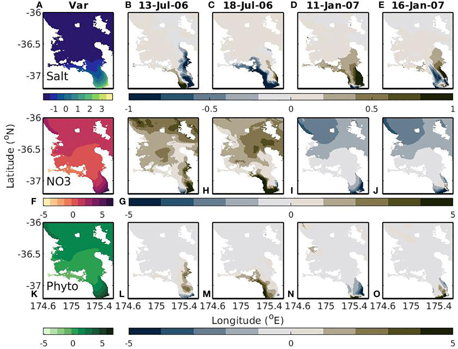
Figure 10 Variability (left; A, F, K) and snapshots of model outputs (right 4 panels; B, E, G–J, L–O; date shown in title). The snapshots show deviations from the mean where a positive (negative) value means the snapshot is greater (less) than the mean. Dates were chosen to demonstrate different river plume positions. Top to bottom rows show salt (g kg^-1), NO₃ (mmol m^-3), and phytoplankton (mmol m^-3). This is for the time-varying-river scenario.

4 Discussion

4.1 Which regions are susceptible to changes in environmental drivers?

The results presented here investigate two sources of nutrients into the Hauraki Gulf region: cross-shelf exchange and riverine inputs. The largest sources of nutrients into this system come from cross-shelf exchanges; however, the dominant source of nutrients differs spatially across the region. The offshore supply of nutrients tends to dominate in the outer Hauraki Gulf and the riverine inputs of nutrients tend to dominate the Firth of Thames region, a result consistent with the nutrient mass-balance study of Zeldis and Swaney (2018). This result is also consistent with other coastal regions in which there is a diminishing effect of riverine-induced eutrophication as the water moves into the highly variable open ocean waters (Zhang et al., 2007).

By comparing the simulations with and without riverine inputs (time-varying-river versus time-varying-nobio), we can quantify what percentage of biological activity comes from riverine input versus cross shelf exchanges (Figure 11). Most of the system is dominated by cross-self exchange, but riverine inputs dominate in a region near the three main rivers in the Firth of Thames. From this we can identify three regions with differing sources of nutrients and subsequent biogeochemical dynamics (Figure 11). It follows from this that the drivers of change will be different for the different regions. Region 1 (yellow in Figure 11C) is dominated by the riverine inputs of nitrogen into the system and will be affected by changes in riverine inputs. This includes changes in land use and changes in freshwater and nutrient runoff. For example, previous research has shown that this region has already undergone significant changes due to the historical increases in nutrient loading its rivers have received (Snelder et al., 2018; Zeldis et al., 2022). While the time-varying-nobio scenario presented here is an extreme situation to elucidate the sensitivity of the region to the riverine forcing, it is not entirely unrealistic, as the pre-anthropogenic total nitrogen loading was likely lower than the present-day situation by ~85% (Snelder et al., 2018). Region 3 (deep blue in Figure 11C) is dominated by exchanges between the shelf break and the Hauraki Gulf. These exchanges are driven by local and far-field winds and East Auckland Current dynamics (Zeldis et al., 2004; Santana et al., 2021) and, as such, are expected to be more susceptible to biogeochemical conditions affecting those offshore waters, including changes in weather and current patterns that alter cross-shelf exchange of nutrients. Region 2 (green in Figure 11C) has influences from offshore and riverine inputs and will be susceptible to changes in both. These findings indicate that the 3 regions are subject to varying forcing of biogeochemical dynamics, consistent with the regional variation in carbonate and oxygen dynamics described in the observation-based studies of Zeldis and Swaney (2018) and Zeldis et al. (2022).

FIGURE 11

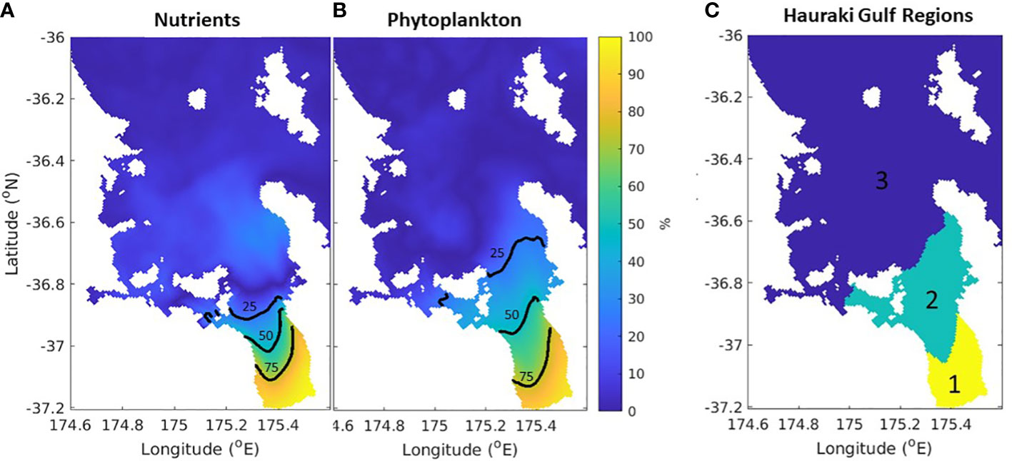
Figure 11 Percentage of surface nutrients (A) and (B) phytoplankton that originated from nutrient loading from rivers in the time-varying-river scenario. The 75%, 50% and 25% contours are shown in black. (C) Schematic of the three regions identified in the text. Biological dynamics are dominated by riverine processes in the yellow region, offshore processes in the blue region and both in the green region.

In addition to long-term changes in oceanic flows and land runoff, regions 1 and 3 have a large variability due to event-scale and weather driven forcing. For region 3, seasonal and interannual scale variability in mesoscale winds are known to modulate the circulation and nutrient dynamics (Sharples and Greig, 1998; Zeldis et al., 2004; Sharples and Zeldis, 2021). For region 1, seasonal to interannual variation in runoff of freshwater and nutrients, potentially driven by climatic variation and land use management changes will be most important (Zeldis and Swaney, 2018). As such, these regions are more susceptible to changes in the frequency and scale of these respective forcings.

4.2 Model representation of organic sediment fluxes

In this model, detritus that sinks past the bottom grid cell is instantly remineralized with a portion being lost from the system due to denitrification. We have followed Fennel et al. (2006) who, based on empirical data, calculated this denitrification flux to be 75% of the detrital matter reaching the bottom grid cell. However, in the Hauraki Gulf, it is possible that this denitrification process is becoming less efficient, leading to less nitrogen loss by this process (Zeldis and Swaney, 2018). Future simulations that investigate long-term changes in denitrification efficiency could investigate this.

The instant remineralization assumption was made for coding simplicity and, whilst it is a common assumption in estuarine and coastal biogeochemical modelling studies (Fennel et al., 2006; Gan et al., 2014; Li et al., 2020; Yu et al., 2021; Tak et al., 2022), its effect on the modelling results needs to be carefully considered. This instant remineralization assumption means that the release of NH₄ from the sediments after a large detrital-deposition event will occur earlier in the model than what would be observed in a real system. In the model, large detrital deposits occur just after the spring and summer blooms, and there is an increase in modelled NH₄ in summer and autumn, particularly in the near bottom layers. However, in the observations the NH₄ maxima occur during the summer and winter months, suggesting that the timing of the modelled bottom NH₄ peak in autumn is affected by the instant remineralization assumption. It follows that the seasonal cycle of denitrification (Figure 9) could also be offset from that which is occurring in the real system. Accordingly, we have refrained from further investigations of seasonally resolved estimates of nitrogen fluxes for this region in this study. Whilst these model/data differences do not invalidate the results presented here, the instant remineralization assumption needs to be considered for future applications of this model.

There are more complex benthic parameterizations and models that can be used to represent benthic fluxes (e.g., Moriarty et al., 2017), but without the data to constrain and assess these it is unclear if they will improve the representation of the system. Future work should focus on collection of data to understand the behavior of sediment and denitrification fluxes for this system.

4.3 Estimates of seasonal averages from sparse observations

The observational dataset used here was a long-term, spatially resolved survey where discrete seasonally resolved samples have been used to create climatologies for the Hauraki Gulf. In this work, two modelled climatologies have been used to understand the uncertainties introduced by sampling bias in the observed climatology (Figures 3–5 and Section 3.13). We created a modelled climatology that has been subsampled (temporally and spatially) to represent a similar sampling regime as the observed climatology and compared this with a modelled climatology created using all available model outputs. We found that there were differences between them, which suggests that the sampling regime used to collect the real-world observations is biased by event scale processes, or that the model has far greater variability than seen by the observations. These uncertainties need to be considered when interpreting the processes captured in the modelled and observed climatologies.

The most notable difference between the modelled subsampled and the full climatology comparisons is in the summer where the modelled subsampled climatology has an along-transect gradient in chlorophyll and homogeneously mixed NO₃ whereas the modelled full climatology has subsurface maxima in chlorophyll and NO₃. This suggests that the interannual variability in biological properties in summer is large enough that our sampling regime does not fully capture this variability. Zeldis et al. (2022) shows that there is interannual variability in the onset of the subsurface bloom with the onset occurring anytime between summer and autumn. We suggest that more intensive sampling around this period will better enable us to understand and represent this process in our models and observational climatologies.

4.4 Model and data comparisons

With the potential uncertainties introduced in the sampling methods in mind, the model performance was assessed against those data. Three variables were compared over four seasons, giving 12 different comparisons. Ten of these comparisons were shown to reproduce features analogous to those observed or had large uncertainties in the observational sampling methods. Two of the comparisons showed little difference between the two different modelled climatologies, but a big difference between the modelled climatologies and observations. The low differences between true and subsampled modelled climatologies suggest that observational sampling techniques were not adding biases to the climatology, and these differences occur due to systematic model errors. The comparisons under question were for winter NH₄ and autumn chlorophyll. Winter NH₄ is likely due to the above-mentioned biases introduced with a simplified representation of sediment processes. The model does not capture a subsurface chlorophyll bloom in autumn. Zeldis et al. (2022) shows that this autumn subsurface chlorophyll bloom is driven by a stratification of the water column. Whilst the model’s temperature and salinity perform well against the observed timeseries in autumn, the coarse resolution of these data in the vertical means that the assessment of the modeled vertical stratification is also imperfect due to the coarse vertical resolution. As such, we suggest that the vertical stratification and other factors such as parameterizations involving phytoplankton growth, zooplankton grazing and chlorophyll to mass ratios in phytoplankton during autumn need to be further investigated to understand the modelled autumn chlorophyll.

Figure 2 shows that the maximum errors in modelled temperature occur in late winter/early spring which suggests that heat fluxes are not well represented during this time. In addition to this, Figure 3 shows that modelled spring nitrogen is well mixed throughout the water column whereas observations show that surface nitrogen is depleted. Combined, this suggests that the model is not capturing water column dynamics such as stratification during this time. We suggest that future work should also investigate atmospheric fluxes during spring to better capture this process.

In Figure 8 we show that there is about a 4 mg m^-3 change in chlorophyll between the time-varying river and no river simulations. However, the model underestimated the chlorophyll by about 1-2 mg m^-3 in autumn. Autumn makes up 25% of the model outputs so we estimate that the modelled autumn bias could add up to 15% to these results.

Other sedimentary processes that are not captured by the model, or covered by the observations, include those occurring on the tidal-flat and shallow (<5m deep) areas about 2-4 km offshore near the three main rivers in the inner Firth of Thames. Whilst there is no evidence that missing this process is creating a wide-spread modelled overestimation of phytoplankton growth, future work investigating this process could help inform the model’s estimation of phytoplankton growth in the Firth of Thames region.

5 Summary and future work

The results indicate that both observational and modelling estimates of the Hauraki Gulf system have their benefits and drawbacks. Here we combine the two to understand the limitations of each and provide a better overall picture of the dynamics of the Hauraki Gulf. The biogeochemical model expands on previous observation and mass-balance modelling studies of the biogeochemistry of the region (Zeldis and Swaney, 2018; Zeldis et al., 2022) by adding spatial and temporal resolution to the description. From this we have ascertained that there are three main biological regions in the Firth of Thames: riverine dominated, offshore exchange dominated and an intermediate transition zone incorporating much of the Hauraki Gulf. However, there is also a large temporal variability in this system.

The model was used to assess the observed sampling regime to ensure that it was not biased by event-scale variability. It was found that the sampling regime was mostly adequate to remove biasing due to event scale processes, however more data needs to be collected during the summer months to better understand the biases during these times. The representation of fluxes between the sediments and the water column is a process that should be considered for observational studies combined with future model development. When combined, models and observations can provide complementary views of the system and can assist in informing each other’s methodologies and interpretation of results. It forms a basis for investigations of environmental impacts and stressors in the region, including assessing the relative impacts of terrestrial and oceanic forcing of the system and informing limit setting for catchment nutrient runoff.

Data availability statement

The data presented in the study are deposited in SEANOE, accession link: https://doi.org/10.17882/95173.

Author contributions

HM performed most of the model setup, analysis and wrote the article. CC calculated observed climatologies and provided intellectual input. DP created the time-varying riverine inputs into the model and provided intellectual input. JZ oversaw field data collection and provided intellectual input. NB provided intellectual input. All authors contributed to the article and approved the submitted version.

Funding

This work was supported by the Ministry of Business, Innovation and Employment (MBIE) Strategic Science Investment Fund and The Coastal Acidification: Rate, Impacts and Management (CARIM) project which was funded by the New Zealand Ministry of Business, Innovation and Employment (C01X1510).

Acknowledgments

The authors would like to acknowledge Mark Hadfield and the ROMS developers for code used in setting up and analyzing the model used in this work.

Conflict of interest

The authors declare that the research was conducted in the absence of any commercial or financial relationships that could be construed as a potential conflict of interest.

Publisher’s note

All claims expressed in this article are solely those of the authors and do not necessarily represent those of their affiliated organizations, or those of the publisher, the editors and the reviewers. Any product that may be evaluated in this article, or claim that may be made by its manufacturer, is not guaranteed or endorsed by the publisher.

Supplementary material

The Supplementary Material for this article can be found online at: https://www.frontiersin.org/articles/10.3389/fmars.2023.1117794/full#supplementary-material

References

Aumont O., Éthé C., Tagliabue A., Bopp L., Gehlen M. (2015). PISCES-v2: an ocean biogeochemical model for carbon and ecosystem studies. Geosci. Model. Dev. 8 (8), 2465–2513. doi: 10.5194/gmd-8-2465-2015

CrossRef Full Text | Google Scholar

Booker D. J., Woods R. A. (2014). Comparing and combining physically-based and empirically-based approaches for estimating the hydrology of ungauged catchments. J. Hydrol. 508, 227–239. doi: 10.1016/j.jhydrol.2013.11.007

CrossRef Full Text | Google Scholar

Carstensen J., Conley D. J. (2019). Baltic Sea Hypoxia takes many shapes and sizes. Limnol. Oceanogr. Bull. 28, 125–129. doi: 10.1002/lob.10350

CrossRef Full Text | Google Scholar

Chapman D. C. (1985). Numerical treatment of cross-shelf open boundaries in a barotropic coastal ocean model. J. Phys. Oceanogr 15 (8), 1060–1075. doi: 10.1175/1520-0485(1985)015<1060:NTOCSO>2.0.CO;2

CrossRef Full Text | Google Scholar

Chassignet E. P., Hurlburt H. E., Metzger E. J., Smedstad O. M., Cummings J. A., Halliwell G. R., et al. (2009). US GODAE: global ocean prediction with the HYbrid coordinate ocean model (HYCOM). Oceanography 22 (2), 64–75. doi: 10.5670/oceanog.2009.39

CrossRef Full Text | Google Scholar

Costanza R., d'Arge R., De Groot R., Farber S., Grasso M., Hannon B., et al. (1997). The value of the world's ecosystem services and natural capital. Nature 387 (6630), 253–260. doi: 10.1038/387253a0

CrossRef Full Text | Google Scholar

Davies-Colley R. J., Smith D. G., Ward R. C., Bryers G. G., McBride G. B., Quinn J. M., et al. (2011). Twenty years of new zealand’s national rivers water quality network: benefits of careful design and consistent operation 1. J. Am. Water Resour. Assoc. 47 (4), 750–771. doi: 10.1111/j.1752-1688.2011.00554.x

CrossRef Full Text | Google Scholar

Fennel K., Wilkin J., Levin J., Moisan J., O'Reilly J., Haidvogel D. (2006). Nitrogen cycling in the middle Atlantic bight: results from a three-dimensional model and implications for the north Atlantic nitrogen budget. Glob. Biogeochem. Cycles 20 (3), GB3007. doi: 10.1029/2005GB002456

CrossRef Full Text | Google Scholar

Gan J., Lu Z., Cheung A., Dai M., Liang L., Harrison P. J., et al. (2014). Assessing ecosystem response to phosphorus and nitrogen limitation in the pearl river plume using the regional ocean modeling system (ROMS). J. Geophys. Res. Oceans 119, 8858–8877. doi: 10.1002/2014JC009951

CrossRef Full Text | Google Scholar

Giani M., Djakovac T., Degobbis D., Cozzi S., Solidoro C., Umani S. F. (2012). Recent changes in the marine ecosystems of the northern Adriatic Sea. Estuarine Coast. Shelf Sci. 115, 1–13. doi: 10.1016/j.ecss.2012.08.023

CrossRef Full Text | Google Scholar

Glenn S., Arnone R., Bergmann T., Bissett W. P., Crowley M., Cullen J., et al. (2004). Biogeochemical impact of summertime coastal upwelling on the new Jersey shelf. J. Geophys. Res. Oceans. 109 (C12), C12S02. doi: 10.1029/2003JC002265

CrossRef Full Text | Google Scholar

IPCC (2019). Summary for policymakers. in: IPCC special report on the ocean and cryosphere in a changing climate. Eds. Po ürtner H.-O., Roberts D. C., Masson-Delmotte V., Zhai P., Tignor M., Poloczanska E., Mintenbeck K., Alegri ía A., Nicolai M., Okem A., Petzold J., Rama B., Weyer N. M. (NY, USA: Cambridge University Press, Cambridge, UK and New York), 755. doi: 10.1017/9781009157964

CrossRef Full Text | Google Scholar

Jolliff J. K., Kindle J. C., Shulman I., Penta B., Friedrichs M. A., Helber R., et al. (2009). Summary diagrams for coupled hydrodynamic-ecosystem model skill assessment. J. Mar. Syst. 76 (1-2), 64–82. doi: 10.1016/j.jmarsys.2008.05.014

CrossRef Full Text | Google Scholar

Kalnay E., Kanamitsu M., Kistler R., Collins W., Deaven D., Gandin L., et al. (1996). The NCEP/NCAR 40-year reanalysis project. Bull. Am. Meteorol. Soc. 77 (3), 437–471. doi: 10.1175/1520-0477(1996)077<0437:TNYRP>2.0.CO;2

CrossRef Full Text | Google Scholar

Karthik R., Robin R. S., Anandavelu I., Purvaja R., Singh G., Mugilarasan M., et al. (2020). Diatom bloom in the amba river, west coast of India: a nutrient-enriched tropical river-fed estuary. Reg. Stud. Mar. Sci. 35, 101244. doi: 10.1016/j.rsma.2020.101244

CrossRef Full Text | Google Scholar

Kelly S., Kirikiri R., Sim-Smith C., Lee S. (2020) State of our gulf 2020: hauraki Gulf/Tīkapa Moana/Te moana-nui-a-Toi state of the environment report 2020. Available at: https://www.aucklandcouncil.govt.nz/about-auckland-council/how-auckland-council-works/harbour-forums/docsstateofgulf/state-gulf-full-report.pdf.

Google Scholar

Laurent A., Fennel K., Cai W.-J., Huang W.-J., Barbero L., Wanninkhof R. (2017). Eutrophication-induced acidification of coastal waters in the northern gulf of Mexico: insights into origin and processes from a coupled physical-biogeochemical model. Geophys. Res. Lett. 44, 946–956. doi: 10.1002/2016GL071881

CrossRef Full Text | Google Scholar

Li D., Gan J., Hui R., Liu Z., Yu L., Lu Z., et al. (2020). Vortex and biogeochemical dynamics for the hypoxia formation within the coastal transition zone off the pearl river estuary. J. Geophys. Res. Oceans 125 (8), e2020JC016178. doi: 10.1029/2020JC016178

CrossRef Full Text | Google Scholar

Liu K., Yan W., Lee H., Chao S., Gong G., Yeh T. (2015). Impacts of increasing dissolved inorganic nitrogen discharged from changjiang on primary production and seafloor oxygen demand in the East China Sea from 1970 to 2002. J. Mar. Syst. 141, 200–217. doi: 10.1016/j.jmarsys.2014.07.022

CrossRef Full Text | Google Scholar

Lotze H. K., Lenihan H. S., Bourque B. J., Bradbury R. H., Cooke R. G., Kay M. C., et al. (2006). Depletion, degradation, and recovery potential of estuaries and coastal seas. Science 312 (5781), 1806–1809. doi: 10.1126/science.112803

PubMed Abstract | CrossRef Full Text | Google Scholar

McLeod I. M., Parsons D. M., Morrison M. A., Le Port A., Taylor R. B. (2011). Factors affecting the recovery of soft-sediment mussel reefs in the firth of Thames. Mar. Freshw. Res. 63 (1), 78–83. doi: 10.1071/MF11083

CrossRef Full Text | Google Scholar

Moriarty J. M., Harris C. K., Fennel K., Friedrichs M. A., Xu K., Rabouille C. (2017). The roles of resuspension, diffusion and biogeochemical processes on oxygen dynamics offshore of the rhône river, France: a numerical modeling study. Biogeosciences 14 (7), 1919–1946. doi: 10.5194/bg-14-1919-2017

CrossRef Full Text | Google Scholar

Muller-Karger F. E., Varela R., Thunell R., Luerssen R., Hu C., Walsh J. J. (2005). The importance of continental margins in the global carbon cycle. Geophys. Res. Lett. 32 (1), L01602. doi: 10.1029/2004GL021346

CrossRef Full Text | Google Scholar

Neumann T., Fennel W., Kremp C. (2002). Experimental simulations with an ecosystem model of the Baltic Sea: a nutrient load reduction experiment. Glob. Biogeochem. Cycles 16 (3), 7–1. doi: 10.1029/2001GB001450

CrossRef Full Text | Google Scholar

Nixon S. W. (1995). Coastal marine eutrophication: a definition, social causes, and future concerns. Ophelia 41 (1), 199–219. doi: 10.1080/00785236.1995.10422044

CrossRef Full Text | Google Scholar

Pendleton L. H., Thébaud O., Mongruel R. C., Levrel H. (2016). Has the value of global marine and coastal ecosystem services changed? Mar. Policy. 64, 156–158. doi: 10.1016/j.marpol.2015.11.018

CrossRef Full Text | Google Scholar

Pinkerton M., Gall M., Wood S., Zeldis J. (2018). Measuring the effects of bivalve mariculture on water quality in northern new Zealand using 15 years of MODIS-aqua satellite observations. Aquac. Environ. Interact. 10, 529–545. doi: 10.3354/aei00288

CrossRef Full Text | Google Scholar

Plew D. R., Zeldis J. R., Dudley B. D., Whitehead A. L., Stevens L. M., Robertson B. M., et al. (2020). Assessing the eutrophic susceptibility of new Zealand estuaries. Estuaries Coasts 43 (8), 2015–2033. doi: 10.1007/s12237-020-00729-w

CrossRef Full Text | Google Scholar

Rabalais N. N., Turner R. E. (2019). Gulf of Mexico hypoxia: past, present, and future. Limnol. Oceanogr. Bull. 28, 117–124. doi: 10.1002/lob.10351

CrossRef Full Text | Google Scholar

Reynolds R. W., Smith T. M., Liu C., Chelton D. B., Casey K. S., Schlax M. G. (2007). Daily high-resolution-blended analyses for sea surface temperature. J. Clim. 20 (22), 5473–5496. doi: 10.1175/2007JCLI1824.1

CrossRef Full Text | Google Scholar

Runkel R. L., Cawford C. G., Cohn T. A. (2004). Load estimator (LOADEST): a Fortran program for estomating constituent loads in streams and rivers (No. 4-A5). Available at: https://pubs.er.usgs.gov/publication/tm4A5.

Google Scholar

Santana R., Suanda S. H., Macdonald H., O’Callaghan J. (2021). Mesoscale and wind-driven intra-annual variability in the East Auckland current. Sci. Rep. 11 (1), 1–11. doi: 10.1038/s41598-021-89222-3

PubMed Abstract | CrossRef Full Text | Google Scholar

Sharples J., Greig M. J. (1998). Tidal currents, mean flows, and upwelling on the north-east shelf of new Zealand. N. Z. J. Mar. Freshw. Res. 32 (2), 215–231. doi: 10.1080/00288330.1998.9516821

CrossRef Full Text | Google Scholar

Sharples J., Zeldis J. R. (2021). Variability of internal tide energy, mixing and nitrate fluxes in response to changes in stratification on the northeast new Zealand continental shelf. N. Z. J. Mar. Freshw. Res. 55 (1), 94–111. doi: 10.1080/00288330.2019.1705357

CrossRef Full Text | Google Scholar

Shchepetkin A. F., McWilliams J. C. (2003). A method for computing horizontal pressure-gradient force in an oceanic model with a nonaligned vertical coordinate. J. Geophys. Res. Oceans 108 (C3), 3090. doi: 10.1029/2001JC001047

CrossRef Full Text | Google Scholar

Shchepetkin A. F., McWilliams J. C. (2005). The regional oceanic modeling system (ROMS): a split-explicit, free-surface, topography-following-coordinate oceanic model. Ocean Model. 9 (4), 347–404. doi: 10.1016/j.ocemod.2004.08.002

CrossRef Full Text | Google Scholar

Snelder T. H., Larned S. T., McDowell R. W. (2018). Anthropogenic increases of catchment nitrogen and phosphorus loads in new Zealand. N. Z. J. Mar. Freshw. Res. 52 (3), 336–361. doi: 10.1080/00288330.2017.1393758

CrossRef Full Text | Google Scholar

Tak Y.-J., Cho Y.-K., Hwang J., Kim Y.-Y. (2022). Assessments of nitrate budgets in the yellow Sea based on a 3D physical-biogeochemical coupled model. Front. Mar. Sci. 8. doi: 10.3389/fmars.2021.785377

CrossRef Full Text | Google Scholar

Walters R. A., Goring D. G., Bell R. G. (2001). Ocean tides around new Zealand. N. Z. J. Mar. Freshw. Res. 35 (3), 567–579. doi: 10.1080/00288330.2001.9517023

CrossRef Full Text | Google Scholar

Wei H., He Y., Li Q., Liu Z., Wang H. (2007). Summer hypoxia adjacent to the changjiang estuary. J. Mar. Syst. 67 (3-4), 292–303. doi: 10.1016/j.jmarsys.2006.04.014

CrossRef Full Text | Google Scholar

Whitehead A. L. (2019). “Spatial modelling of river water-quality state: incorporating monitoring data from 2013 to 2017,” in NIWA client report 2018360CH prepared for the ministry for the environment (NIWA, Christchurch). Available at: https://www.mfe.govt.nz/publications/fresh-water/spatial-modelling-of-river-water-quality-state-incorporating-monitoring.

Google Scholar

Whitehead A. L., Booker D. J. (2019). Communicating biophysical conditions across New Zealand's rivers using an interactive webtool, New Zealand. J. Mar. Freshw. Res. 53, 278–287. doi: 10.1080/00288330.2018.1532914

CrossRef Full Text | Google Scholar

Worm B., Barbier E. B., Beaumont N., Duffy J. E., Folke C., Halpern B. S., et al. (2006). Impacts of biodiversity loss on ocean ecosystem services. Science 314 (5800), 787–790. doi: 10.1126/science.1132294

PubMed Abstract | CrossRef Full Text | Google Scholar

Xue Z., He R., Fennel K., Cai W. J., Hopkinson C. (2013). Modeling ocean circulation and biogeochemical variability in the gulf of Mexico. Biogeosciences 10 (11), 7219–7234. doi: 10.5194/bg-10-7219-2013

CrossRef Full Text | Google Scholar

Yu L., Gan J., Dai M., Hui C. R., Lu Z., Li D. (2021). Modeling the role of riverine organic matter in hypoxia formation within the coastal transition zone off the pearl river estuary. Limnol. Oceanogr. 66, 452–468. doi: 10.1002/lno.11616

CrossRef Full Text | Google Scholar

Zeldis J. R., Currie K. I., Graham S. L., Gall M. P. (2022). Attributing controlling factors of acidification and hypoxia in a deep, nutrient-enriched estuarine embayment. Front. Mar. Sci. 8. doi: 10.3389/fmars.2021.803439

CrossRef Full Text | Google Scholar

Zeldis J. R., Swales A., Currie K., Safi K., Nodder S., Depree C., et al. (2015) Firth of Thames water quality and ecosystem health – data report (Waikato Regional Council and DairyNZ). Available at: https://www.waikatoregion.govt.nz/assets/WRC/WRC-2019/TR201523.pdf (Accessed 11th May 2023).

Google Scholar

Zeldis J. R., Swaney D. P. (2018). Balance of catchment and offshore nutrient loading and biogeochemical response in four new Zealand coastal systems: implications for resource management. Estuaries Coasts 41 (8), 2240–2259. doi: 10.1007/s12237-018-0432-5

CrossRef Full Text | Google Scholar

Zeldis J. R., Walters R. A., Greig M. J., Image K. (2004). Circulation over the northeastern new Zealand continental slope, shelf and adjacent hauraki gulf, during spring and summer. Cont. Shelf Res. 24 (4-5), 543–561. doi: 10.1016/j.csr.2003.11.007

CrossRef Full Text | Google Scholar

Zhang J., Liu S. M., Ren J. L., Wu Y., Zhang G. L. (2007). Nutrient gradients from the eutrophic changjiang (Yangtze river) estuary to the oligotrophic kuroshio waters and re-evaluation of budgets for the East China Sea shelf. Prog. Oceanography 74 (4), 449–478. doi: 10.1016/j.pocean.2007.04.019

CrossRef Full Text | Google Scholar

Zhou F., Chai F., Huang D., Wells M., Ma X., Meng Q., et al. (2020). Coupling and decoupling of high biomass phytoplankton production and hypoxia in a highly dynamic coastal system: the changjiang (Yangtze river) estuary. Front. Mar. Sci. 7. doi: 10.3389/fmars.2020.00259

CrossRef Full Text | Google Scholar