Predicting the regime shift of coastal wetlands based on the bistability features in the intertidal zone: A case study in the Liaohe estuary

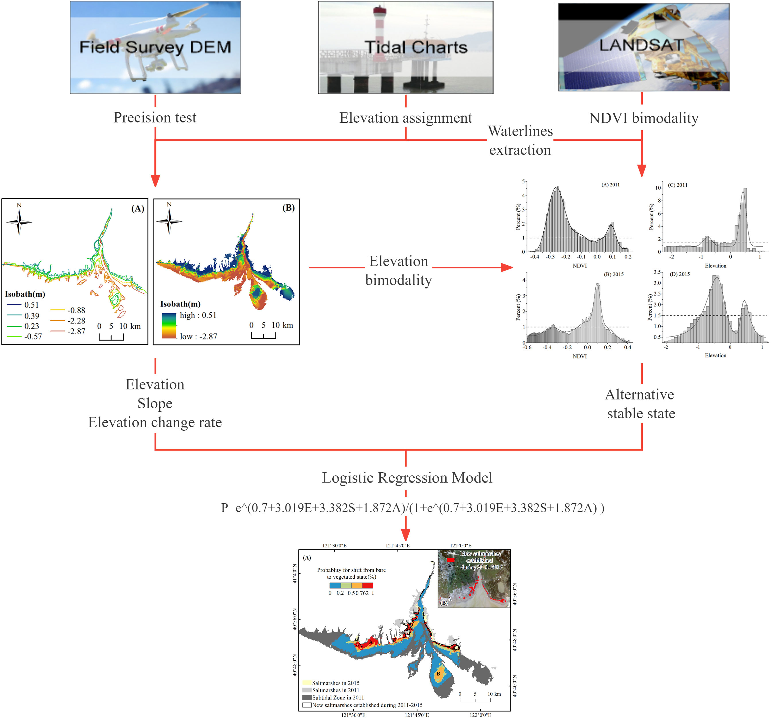
Influenced by human activities and natural interference, the worldwide distribution of coastal wetlands is now undergoing rapid evolution. The prediction on the locations of vegetation conversion is greatly important for the management of these coastal ecosystems in terms of early warning. In this paper, a series of waterlines extracted from multiple satellite images were used to generate a high-precision digital elevation model (DEM) in the intertidal zone of the Liaohe estuary. Based on the characteristics of the alternative stable states in elevation and normalized difference vegetation index (NDVI), the Logistic Regression Model was applied to predict the potential locations of vegetation expansion with geomorphic factors, such as elevation, slope, and annual changing rate of elevation. Before the prediction, the existence of two stable states in the landscape was confirmed in the study area, i.e., low-lying tidal flats and high-lying saltmarshes. When the geomorphic parameters exceeded the thresholds, the stable state transition would occur. By using the Logistic Regression Model, the elevation was the best explainer for determining the vegetation conversion in the single-factor simulation, while the slope was the worst. When multiple factors were integrated in simulations, the prediction with the elevation, slope, and annual elevation change rate was the best, with R² = 0.739, and the overall accuracy of prediction reached 88.6%. The prediction result indicated that the area of saltmarshes in the Liaohe estuary increased by 16.7 km² at a rate of 0.8% per year between 2011 and 2015. When considering the popularization in restoration practice, it is necessary to evaluate the reliability and flexibility of the Logistic Regression Model in predicting vegetation conversion in more types of estuarine wetlands.

GRAPHICAL ABSTRACT

Graphical Abstract

1 Introduction

Coastal saltmarsh is one of the most productive ecosystems which plays an important role in coastal defense by decelerating storm surge flooding (Stark et al., 2015), attenuating waves, and mitigating shoreline erosion (Möller et al., 2014), filtering nutrients and contaminants (Almeida et al., 2011) and providing nursery areas for commercially important fish and shellfish (Costanza et al., 1997; Zhang et al., 2021). Located within the intertidal zone, saltmarshes are shaped by the interactions between vegetation establishment, hydrodynamics, and sedimentation (D'Alpaos et al., 2007; van Belzen et al., 2017). As the global coastal wetlands were characterized in a dynamic state (Scott et al., 2014), the shift from bare flat to vegetated marshes or the opposite transition could occur frequently. In the last 50 years, the coastal wetland worldwide lost more than 50% of their area, at a rate of 0.5% ~ 1.5% per year (Scott et al., 2014). Meanwhile, local increase in saltmarsh areas still occurred frequently in many coasts and estuaries. For example, the Scheldt estuary was mainly dominated by saltmarsh expansion between 1931 and 2004, with large areas’transformation from bare flat to vegetated marshes due to the high sediment accumulation rates and low impact of sea level rise (Wang and Temmerman, 2013).

With the increasing awareness of saltmarsh ecosystem service to estuaries and coasts, it is essential to understand and predict this impending transformation. The effective practice has been focused on how to preserve and restore these coastal wetland ecosystems in recent decades (Xie et al., 2019). Prediction of the change in vegetated areas is benefit for policy decisions in terms of early warning. Great efforts of empirical and numerical models, which integrated current information into the prediction of vegetation evolution, have been invested in detecting the driving or limiting factors on the colonization or spreading of specific saltmarsh species. The driving forces include seed bank deposition, seed germination, seedling dispersal and establishment, and asexual propagation by tiller and rhizome growth (Ge et al., 2013). For instance, the process-based grid model for predicting the spatiotemporal range of S. alterniflora expanding in the Yangtze Estuary was established on the growth processes of single plant individuals (Xie et al., 2021). The Maxent model for predicting the suitable area for S. salsa dispersion in the Liaohe estuary stemmed from the relationship between the known distribution of the species and relevant environmental variables, such as water salinity, Cd, Zn, organic matter, etc. (Cao et al., 2022). Moreover, cellular-automata models considered a set of transition rules (including the habitat characteristics and species interaction) in simulating the expanding process of S.alternifora in discrete time steps after being introduced to the new shoals at Jiuduansha Shoals, Shanghai (Huang et al., 2008). Although the modeling practice promoted the prediction accuracy in vegetation conversion, many numerical models ignored the geomorphic factors in determining vegetation colonization and growth. In view of the landscape, the interaction between elevation and vegetation benefits the landform’s coevolution in the coastal area. On the one hand, the geomorphic feature usually acts as the most important regulator in determining intertidal vegetation zonation in many aspects (Wang and Temmerman, 2013). Owning to the spatial heterogeneity in macro to micro topography, the critical ecological processes in plant populations were influenced, such as seed dispersal, germination preferences, seedling survival, and mortality (Xie et al., 2019). Elevation-related subsistence environments, such as surface water redistribution, water retention duration and water flow direction, soil moisture, redox potential, soil salinity, and nutrient effectiveness also affect the establishment of plant propagules (Pennings and Callaway, 1992; Bouma et al., 2005; Davy et al., 2011; Moeslund et al., 2013; Karstens et al., 2016). On the other hand, the increasing elevation of coastal wetlands is mainly achieved by accumulating organic and inorganic material and reducing erosion after the vegetation establishment (Wang G, et al., 2016). Through the accumulation and decomposition of above-ground deadfall, the vegetation promotes the elevation by the accumulation of organic deposition. The velocity of water flow can be also reduced through the above-ground part of the saltmarsh, which in turn affects the external sediment deposition process (Baustian et al., 2012). In addition, the underground part of the plant can significantly influence the soil volume of the rhizosphere through root growth and decomposition processes, which can maintain or even increase the marsh elevation and help resist the erosive forces of storm-generated waves and tides (Baustian et al., 2012).

Obtaining elevation information on vast and inaccessible intertidal areas is a challenging and expensive task. Traditional survey methods, such as ground and ship-based surveys, are difficult to implement in the shoal environment owing to severe weather, complex topography, and variable tidal conditions. LiDAR (Light Detection and Ranging) and InSAR (Interferometric Synthetic Aperture Radar) need expensive and time-consuming regular maintenance. It is difficult for Lidar to obtain large-scale simultaneous DEMs under changing tidal conditions and for InSAR to produce accurate vertical accuracy due to the low-coherence interferometry in a wet environment (Ryu et al., 2008; Guo et al., 2010; Baier et al., 2018). Compared with these methods, Waterline detection method is considered as an effective method for generating intertidal topography which uses the changing boundary between the water body and the tidal flats. The position of the waterline represents the tidal height at the satellite overpass moment which is considered as quasi-contour line of the topography (Kang et al., 2017). The waterline detection method has been widely applied in many regions around the world, such as the Australia Coast (Sagar et al., 2017), Gomso Bay in Korea (Ryu et al., 2002), Yangtze Delta in China (Zhao et al., 2008), etc.

Multistability is one of the manifested features in coastal areas, i.e., the coastal system can exist in more than one stable state with completely contrasting structures and functions in very limited areas (Scheffer and Carpenter, 2003). As vegetated and bare flats can be considered as alternative states of intertidal ecosystems, van Belzen et al. (2017) revealed an intermediate elevation between the high biomass saltmarsh state and a low biomass tidal flat state in combination with experimental and observational data within the range of the Western Scheldt estuary (van Belzen et al., 2017). The locations where the transition from bare flat to saltmarshes could be predicted by using the Logistic Regression Models (Wang and Temmerman, 2013), which included physical parameters, such as elevation, tidal currents, and wave orbital velocities (Wang and Temmerman, 2013). With respect to model complexity for popularization, the common existence of alternative stable states in the coastal landscape has potential advantages in predicting the evolution process in the landscape.

The Suaeda salsa saltmarsh is a typical estuarine wetland along the coast of the Bohai sea, which provides an important stopover habitat for migratory shorebirds on the migration route from East Asia to Australia. The Liaohe estuarine wetland belongs to one of the most important transit stations and destinations. From 1976 to 2004, saltmarshes in the Liaohe estuary decreased by 45%. Afterward, the indigenous S. salsa in the delta increased due to the increase of the annual average sand transport and runoffs during 2007-2009 (Gu et al., 2018). However, to what extent the geomorphic driver acts on shaping the coastal wetlands has not been scientifically validated. Accordingly, the objectives of this study are as follows. 1) to refine the geomorphic features in determining the potential state shifts from the bare to vegetated state at a landscape scale of the Liaohe estuary; 2) To optimize geomorphic parameters in the Logistic Regression Models, such as elevation, slope, and change rate in elevation for the best prediction of vegetation conversion; 3) To assess the practice scope of the Logistic Regression Model in predicting the locations of vegetation conversion in the estuarine wetlands.

2 Study area and datasets

2.1 Study area

The Liaohe estuary, located in Northeast China, is adjacent to the northern Liaodong Bay of the Bohai Sea within the range of 121°35’~122°55’E and 40°40’~41°25’N (Figure 1). It is a tide-dominated estuary, with an irregular and semi-diurnal tide, an average tidal range of 2.7 m, and dominant tidal currents from northeast to southwest (Zhu et al., 2010). Several large rivers, including the Liaohe River, Daliao River, Daling River, etc., run into the sea with a total of 11.7 billion m³ of water per year. 76 million tons of sediment are deposited in the delta annually (Xiao and Li, 2004). The climate is controlled by the semi-humid temperate monsoon. Mean annual precipitation is 612 mm, with 70%-80% concentrated in summer (from July to September). Annual average evaporation is 1669.60 mm, which could be more than ten times higher than precipitation in spring (Lang et al., 2012; Li et al., 2014). The temperature ranged from -10.4°C in January to 27.4°C in July, with a mean annual of 8.3°C. The frost-free period is about 175 days per year (Wang et al., 2017; Li et al., 2021).

FIGURE 1

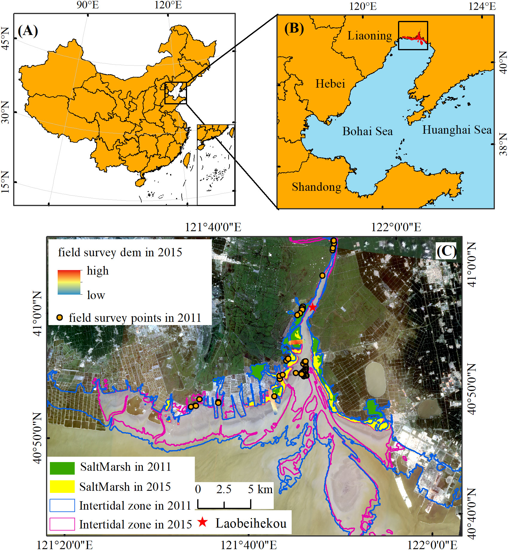
Figure 1 The location of Liaohe estuary (A, B) and the range of intertidal features in 2011 and 2015 (C). The red star refers to Laobeihekou Tidal Gauge Station. The background image was captured by the GaoFen satellite in 2020. The boundary of intertidal zones (the blue line for 2011 and the pink line for 2015) and the saltmarsh distribution (the green area for 2011 and yellow area for 2015) was derived from the “Tidal Flats Dataset Covers Coastal Region in North of 18°N Latitude of China (1989-2020) (Hu et al., 2021).

Within the transition zone between the Bohai Sea and the upper land, the convergence of fresh and salty water in the Liaohe estuary affected the benthic environmental settings and the succession of natural wetlands as well. The dominant plant species in the intertidal zones of the Liaohe estuary is S. salsa. Liaohe estuary is experiencing elevation changes recently, ranging from a net increase of 0.3 mm yr^-1 to 6.9 mm yr^-1 relative to the mean sea level rise rate of the Bohai Sea, which suggests that S. salsa marshes could keep pace with the sea level rise and maintained the expanding trend (Wang G, et al., 2016).

2.2 Datasets

2.2.1 Satellite image

The raster data covering the study were derived from the Landsat-5, Landsat-7, and Landsat-8 surface reflectance images based on the Google Earth Engine. 17 images with cloud-free and clear waterlines were selected visually, corresponding to the path/row 120/031 of Landsat 5 TM, Landsat 7 ETM+, and Landsat 8 OLI. Although several Landsat 7 ETM+ images were collected in the Scan Line Corrector off (SLC-off) model after May 2003, they were acceptable for interpreting the waterlines because the non-data strips were no more than 3 pixels in width, perpendicular to the coastline in the study areas. The dashed waterlines caused by this error were interpolated from the surrounding solid waterlines (Tong et al., 2020). As the images from Landsat Surface Reflectance were High-Level Data products (level L1T) of the United States Geological Survey (USGS), the atmospheric and topographic effects are minimized in these images. 3 sets of images collected for the temporal interpretation are shown in Table 1.

TABLE 1

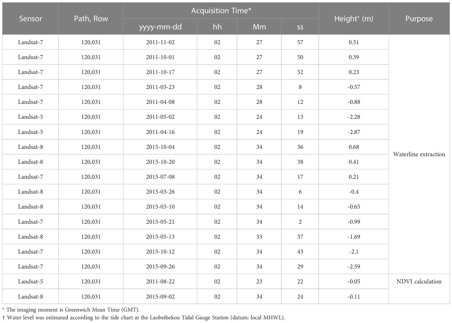
Table 1 Remote sensing images used for waterline extraction and NDVI calculation.

2.2.2 Tidal charts and field survey datasets

The tidal charts in 2011 and 2015 at the Laobeihekou were used to assign the elevation to the instantaneous water boundary in the serial images. The datum of tidal charts is 209 cm below the local mean water level. The datum of measured points in 2011 is the same as the tidal charts. However, the datum of measured stripe DEM in 2015 is the Chinese National Height Datum 1985 which is about 42.8 cm above the local mean water level (Yu et al., 1989). Before the coupling, the datum of all the datasets was corrected to the local MHWL which is 137 cm above the local mean water level in the tidal chart of 2011 at Laobeihekou tidal gauge station. The local MHWL determined the frequency, depth, and duration of tidal inundation which was expected to affect the establishment, survival, and growth of the plant.

3 Data processing

3.1 Waterline extraction and DEM building

With the daily tidal level changing, the boundaries of the unsubmerged tidal flats (i.e., waterlines) move back and forth periodically. The shifting waterlines in the time-series satellite images act as different contours within the intertidal topography (Heygster et al., 2010). In order to extract the waterline in the serial satellite images, the modified normalized difference water index (MNDWI), which was proposed by Hanqiu Xu (Xu, 2007), was calculated as formula (1).

$\begin{array}{ll}\text{MNDWI}=\frac{Green-Mir}{Green+Mir}& (1)\end{array}$

where Green denotes the Green band and Mir denotes the Middle infrared band. The Green and Mir were represented by band 2 and band 5 for Landsat TM and ETM+, and bands 3 and 6 for Landsat OLI respectively.

The maximum variance of MNDWI value among the neighbor lattice cells acted as an adaptive threshold. It is a nonparametric and unsupervised method for determining the threshold automatically in picture segmentation, which is called Otsu (Otsu, 1979). In this way, the optimal threshold was used to segment the image into two classes based on the histogram of imagery, and the boundary was extracted as the waterline.

The serial waterlines were sorted by the specific horizontal position and elevation change (Yong et al., 2021). The elevation assignment of each waterline at the overpass time of the satellite was determined by dating from the tidal chart of the Laobeihekou gauge station. Consequently, the fine DEM of the Liaohe estuary in 2011 and 2015 was generated by using the kriging interpolation on the stacking waterlines.

The slope was calculated in the ArcMap software based on DEM and the annual elevation change rate was the ratio of elevation difference and time difference during 2011-2015.

3.2 Spatial distribution of intertidal vegetation

The frequency distribution of intertidal NDVI and elevation was demonstrated to confirm whether the bimodality of the two stable states occurred (Scheffer and Carpenter, 2003). Assuming two stable states exist, the spatial variation of NDVI would abruptly increase from low values (bare state) to high values (vegetated state) when the elevation exceeded the threshold. Similarly, the spatial variation of elevation was considered as a function of NDVI, which also shifted by the abrupt change from the bare to vegetated state in the intermediate zone (Wang C, et al., 2020).

The pixel-based NDVI values in images of 2011 and 2015 were calculated by the formula (2) and used to construct the frequency distribution curve of the NDVI and elevation.

$\begin{array}{ll}\text{NDVI}=\frac{NIR-R}{NIR+R}& (2)\end{array}$

Where NIR and R denote the Near-infrared band and Red band. The R and NIR were represented by bands 3 and 4 in Landsat-5 and Landsat-7 but by bands 4 and 5 in Landsat-8.

3.3 Prediction of new saltmarsh based on the Logistic Regression Model

Multiple Logistic Regression models were used to predict the shift from bare flat to vegetated marshes between 2011 and 2015. Details in constructing the model were followed by the references (Augustin et al., 2001; Calef et al., 2005; Wang and Temmerman, 2013). Any geomorphic factors associated with saltmarsh expansion could be added in the form of regression equations to obtain ideal simulation results. The expression is presented as follows:

$\begin{array}{ll}P=\frac{e^{b_0+b_1{x}_1+b_2{x}_2+\dots b_m{x}_m}}{1+e^{b_0+b_1{x}_1+b_2{x}_2+\dots b_m{x}_m}}& (3)\end{array}$

Where x represents the variable involved in the binary Logistic Regression Models. Elevation and slope were considered as the key geomorphic variables controlling the survival and establishment of vegetation on intertidal flats (Blott and Pye, 2004; Kim et al., 2017). The elevation and the slope of 2011, and the annual change rate of elevation were selected as explanatory variables in the Logistic Regression Model. Multicollinearity test on the selected variables was completed beforehand, by using the SPSS, which ensured no significant collinearity existing.

The optimal threshold was determined by the Youden index for the occurrence of new marshes as the following formula (Garcia et al., 1995; Vilar del Hoyo et al., 2011; Jiménez-Valverde, 2012; Chang et al., 2013).

$\begin{array}{ll}\text{Youden index }=\text{ Sensitivity }+\text{ specificity}-1& (4)\end{array}$

Where sensitivity is the proportion of true positives that are predicted as events, while specificity is the proportion of true negatives that are predicted as non-events (Catry et al., 2009). When the Youden index was applied in the Logistic Regression Model for predicting the state shift, the sensitivity was the correct percentage for new marshes, while the specificity was the correct percentage for bare flat remaining.

In order to predict the conversion of bare flats into vegetation, those bare areas in the intertidal zone of 2011 were subsequently classified into dichotomous parts, one part staying bare between 2011 and 2015 and the other part being shifted into saltmarsh between 2011 and 2015. Instead, the model was not applied in predicting the conversion of saltmarshes parallelly, because the conversion area from saltmarsh into the tidal flat was small (with the area of about 2.57 km² in total) and sporadic distribution based on the interpretation of remote sensing images.

Since the minimum resolution of the images used in the study is 30m, the new raster data with a grid size of 30 m × 30 m, including “new marsh” and “bare flat”. Nagelkerke R² was calculated to evaluate the simulations, so was the accuracy (%) for new marshes, bare flats, and the whole study area.

4 Results

4.1 The characteristics of DEMs constructed by using the waterline method

The DEMs in 2011 and 2015 were constructed by kriging interpolation on the stacking 7 and 10 waterlines respectively, which were shown in Figures 2, 3. The elevation range of the waterlines was between -2.87m and 0.51m in 2011 and between -2.59m and 0.68m in 2015. Both DEMs demonstrated a gradually increasing from the estuary to the upper land. The DEMs were verified by the field survay datasets. The linear fitting curves of the simulated points and the field measured points were obtained (Figure 4), with R² of 0.72 and 0.85, and RMSE of 0.73 m and 0.51 m, for 2011 and 2015 respectively. The accuracy is accaptable for this study.

FIGURE 2

Figure 2 The extracted waterlines (A) and interpolated DEM (B) in 2011.

FIGURE 3

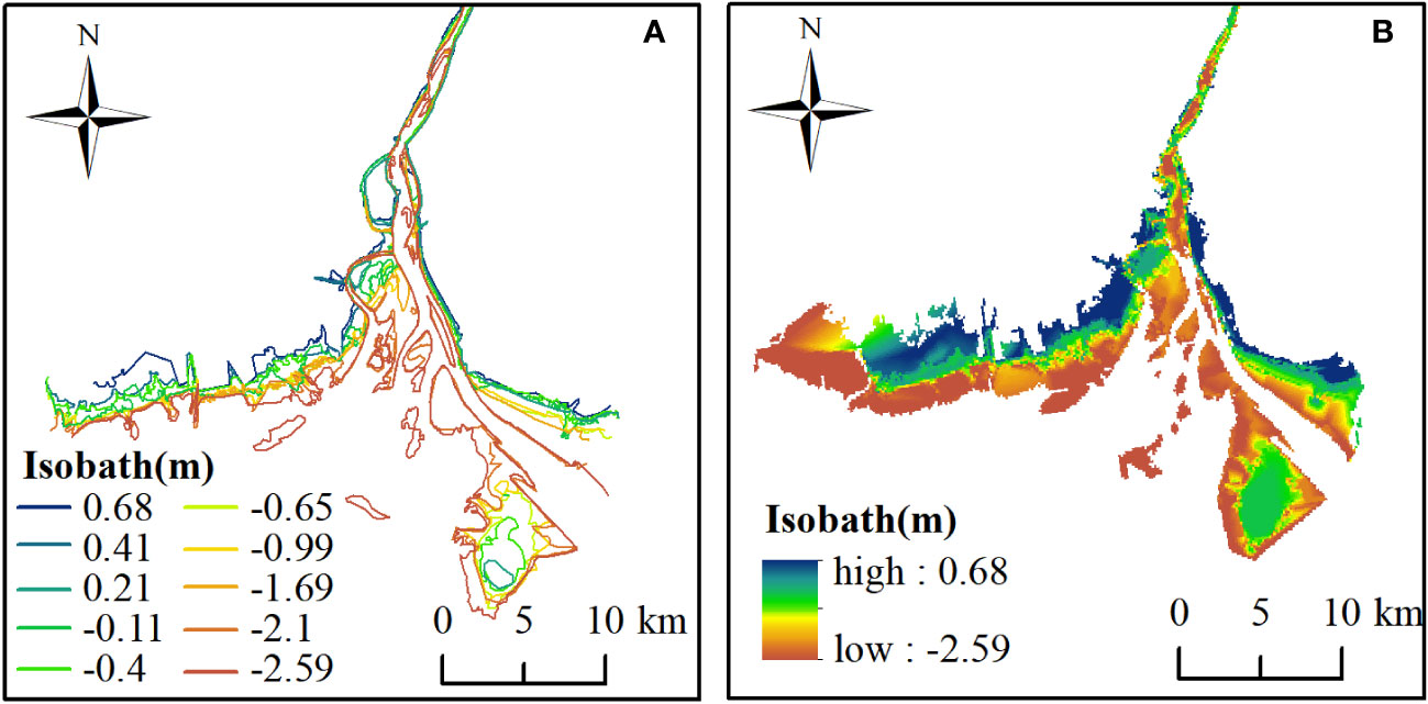
Figure 3 The extracted waterlines (A) and interpolated DEM (B) in 2015.

FIGURE 4

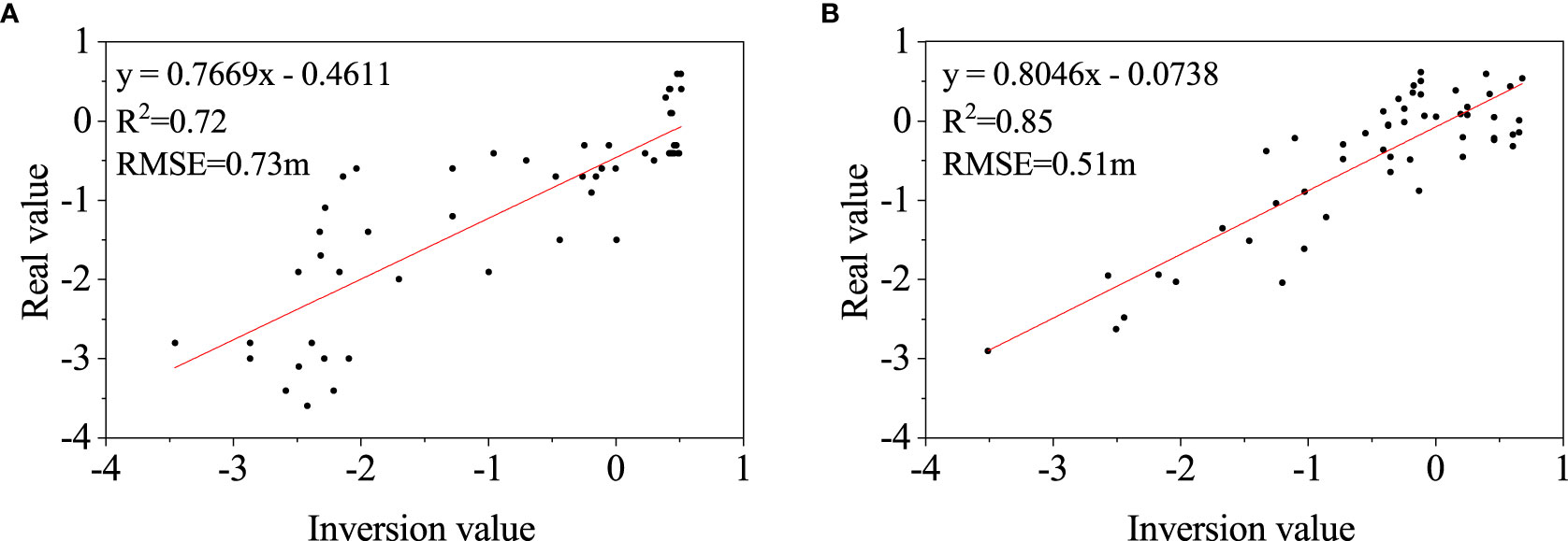
Figure 4 Linear relationships between the interpolated DEM and the measurement values in 2011 (A) and 2015 (B).

4.2 Spatial distribution of biomass, elevation, and slope

4.2.1 Bimodality in biomass distribution and elevation distribution

The frequency distribution of NDVI indicated a bimodal distribution (Figures 5A, B). The positions of the two peaks are at -0.25 and 0.1 in 2011 and -0.34 and 0.11 in 2015, respectively. The left peak of negative NDVI values was controlled by bare flats, while the right peak was dominated by saltmarshes with high vegetation biomass. The frequency of intermediate NDVI values between the two peaks was low.

FIGURE 5

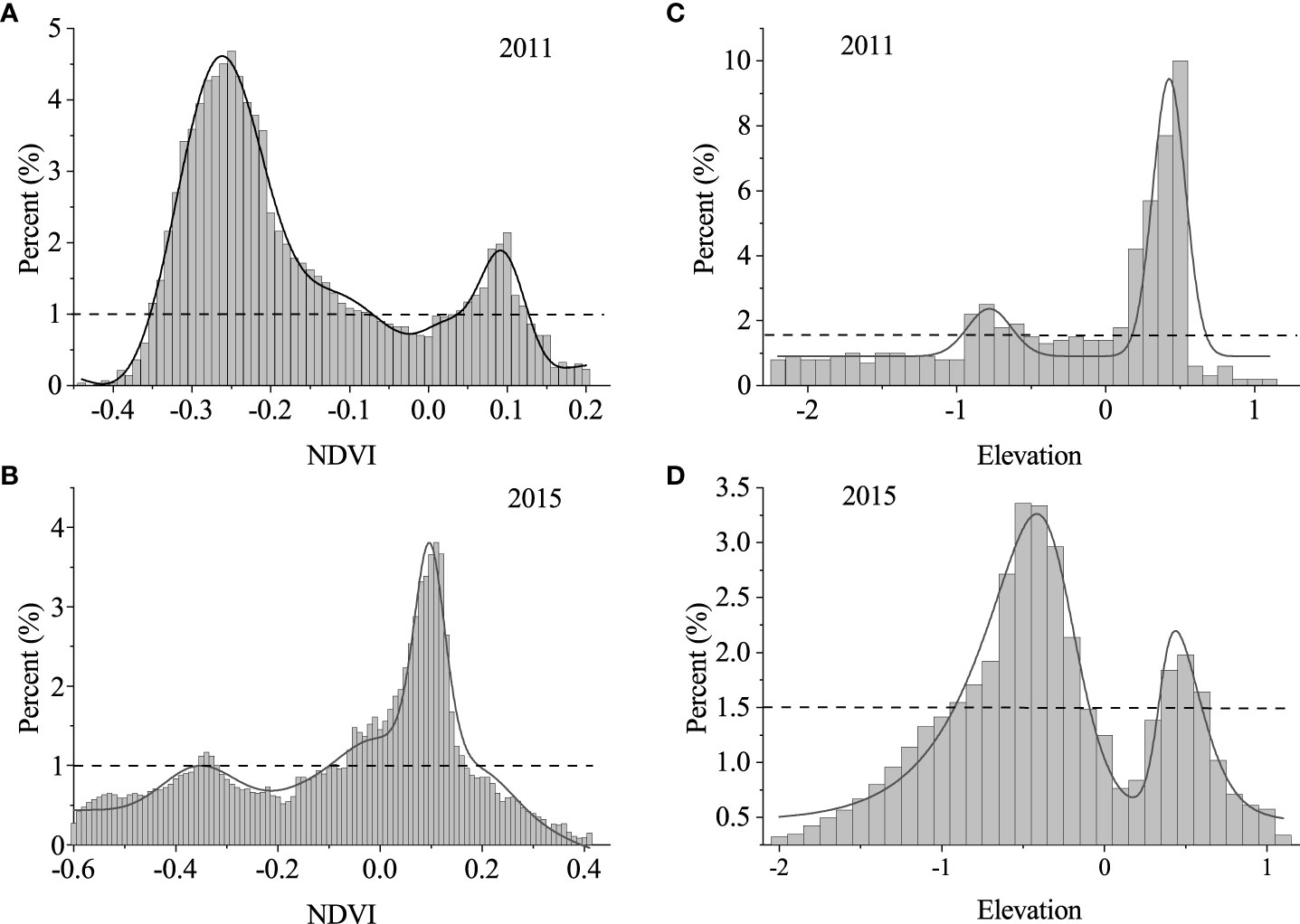
Figure 5 Bimodal frequency distribution of normalized difference vegetation index (NDVI) values and intertidal elevation values in 2011 (A, C) and 2015 (B, D) respectively. The elevation is relative to the mean high water level (MHWL). The proportion on the y-axis is computed as the number of pixels in each NDVI class (every 0.01) or relative elevation class (every 0.1 m) to the total number of pixels involved. The proportion of each NDVI class or elevation class was represented by the bar graph, the curve showed the multi-peak fitting of the proportion. The threshold proportion of NDVI and elevation are 1% and 1.5% (Wang C, et al., 2020), shown in the figure with horizontal black dashed lines. The corresponding instability ranges are from -0.07 to 0.03 and from -0.5 to 0, respectively.

Similarly, the elevation frequency also displayed a bimodal distribution (Figures 5C, D), with two peaks at -0.8 and 0.5 in 2011 and -0.5 and 0.5 in 2015, respectively. The left peak below 0 m (MHWL) was attributed to the low-lying bareflats, while the right narrow peak above 0 m (MHWL) corresponded to the high-lying saltmarshes. Low frequency in the intermediate elevations was observed between the two peaks.

4.2.2 Relationships between variations in elevation and NDVI

According to the instability range provided in Figure 5C, a threshold in elevation was observed at the elevation of -0.5m, where the abrupt shift in NDVI occurred between the bare state and the vegetated state in 2011 (Figure 6A). Below the elevation threshold of -0.5 m, the NDVI varied little with an average value of -0.2. Above the elevation threshold of 0 m, the NDVI remained fairly constant at about 0.25. Accordingly, three elevation zones were demonstrated as “stable low-elevated”, “unstable”, and “stable high-elevated” in Figure 6A. According to the instability range provided in Figure 5A, three NDVI zones were demonstrated as “stable bare”, “unstable”, and “stable vegetated” in Figure 6B.

FIGURE 6

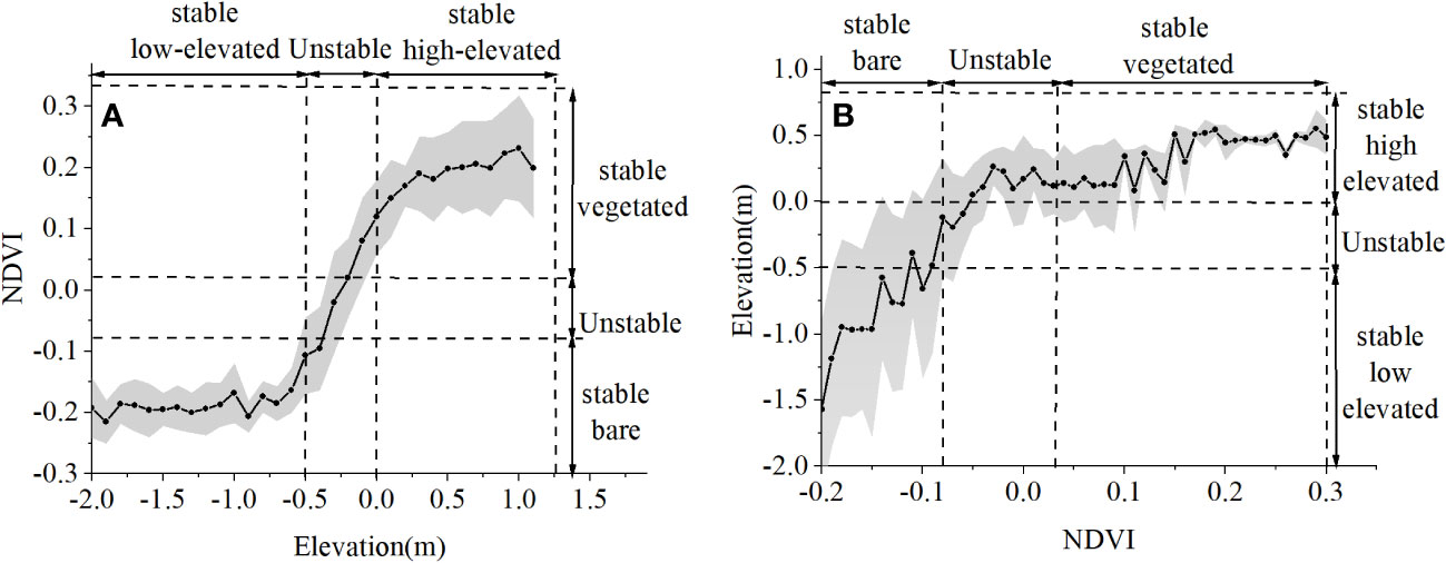
Figure 6 (A) NDVI variation with elevation in 2011. (B) Elevation variation with NDVI in 2011. (A) Black dots denote the mean NDVI value of elevation classes with 0.1 m intervals; the gray area refers to the standard deviation of NDVI for each elevation class. Elevation ranges are indicated (with vertical black-dashed lines) and denoted as “stable low-elevated”, “unstable”, and “stable high-elevated” based on the distribution of elevation in Figure 5C. (B) Black dots denote the mean elevation of NDVI classes with 0.01 intervals; the gray area refers to the standard deviation of elevation for each NDVI class. NDVI ranges are indicated (with vertical black-dashed lines) and denoted as “ stable bare”, “unstable” and “stable vegetated” based on the distribution of NDVI in Figure 5A.

4.2.3 Temporal NDVI change within the unstable elevation zone

The temporal NDVI change was also considered as a function of the elevation. As shown in Figure 7, the average NDVI difference within the elevation interval between 2011 and 2015 increased and then decreased with the increase in elevation. The largest increase in NDVI value was observed in the unstable elevation zone of 2011 as shown in Figure 6A. Furthermore, the stable, low-elevated zone could be divided into two subzones, with the temporal NDVI difference from -0.05 to 0.05 and from 0.05 to 0.20 respectively. The results coincide with the fact that the lower elevation with unstable substrate often influences the colonization success of pioneer vegetation. In contrast, the positive NDVI difference below the elevation threshold in 2011, was attributed to the seaward spreading of vegetation during the period.

FIGURE 7

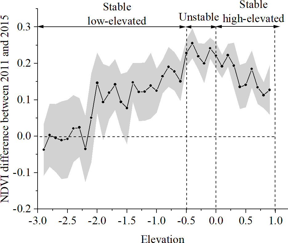
Figure 7 Plot of NDVI difference between 2011 and 2015 and elevation in 2011. Black dots with gray standard deviation denote the mean NDVI change within the 0.1 m elevation interval. The boundaries between the stable and unstable zone in elevation refer to Figure 6A.

4.2.4 Slope variation within different state zones

The spatial distribution of slope performed declined with the increase in NDVI (Figure 8). Within the stable bare zone, the slope was fairly constant at about 0.10°. In contrast, the mean value of the slope declined abruptly from 0.08° to 0.05° within the unstable zone of NDVI in 2011. The slope within the stable vegetated zone gradually decreased from a mean value of 0.05° to 0.01°. The decreasing average slope with the increase of NDVI reflects the benefit of vegetation biomass on the stabilization of the slope as well.

FIGURE 8

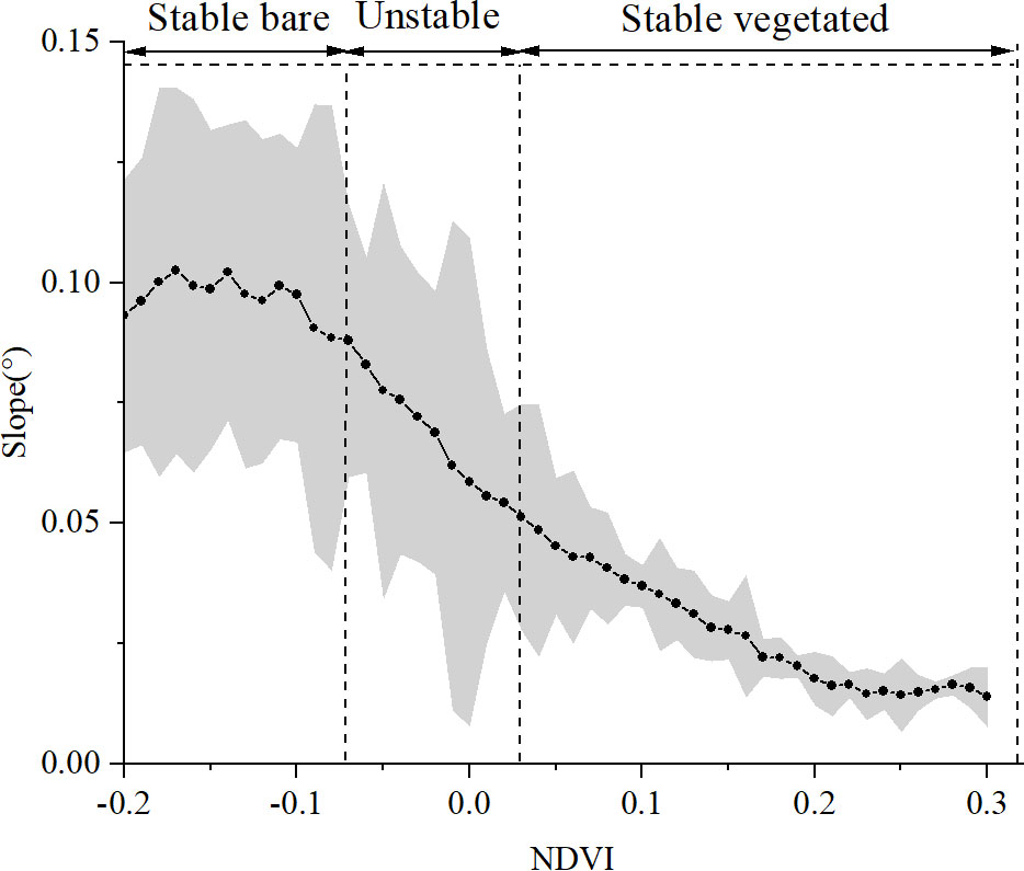
Figure 8 Variation of slope as a function of NDVI in 2011. Black dots in gray standard deviation denote the mean slope change within the NDVI interval of 0.01. The NDVI zonation refers to Figure 6B.

4.3 Prediction on the regime shift

The Logistic regression results indicated the locations (pixels) where bare flats either stayed bare or shifted to saltmarsh between 2011 and 2015. Table 2 showed the 6 prediction models with high significance (p<0.001) by using three variables, i.e., elevation, the annual change rate of elevation, and slope. The VIF values of the three factors are less than 10, verifying no multicollinearity relationship between the factors.

TABLE 2

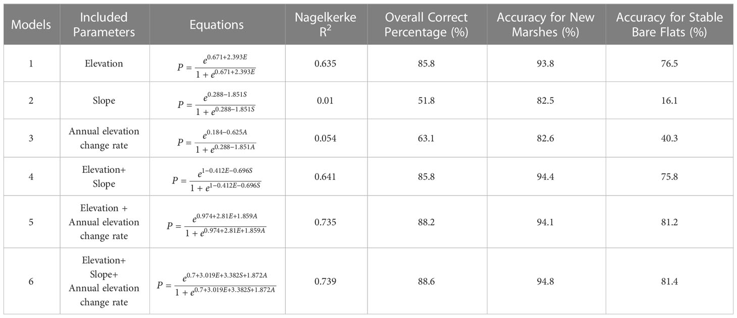
Table 2 Logistic regression models as a function of elevation, the annual change rate of elevation, and slope, with evaluating coefficients.

Elevation was the best single explanatory variable (Model 1; Nagelkerke R² = 0.635), much better than the slope (Model 2; Nagelkerke R² = 0.01) or the annual change rate of elevation (Model 3; Nagelkerke R² = 0.054). The Nagelkerke R² increased considerably when both elevation and annual change rate of elevation were introduced in the model (Model 5; Nagelkerke R² = 0.735), and reached the highest when the slope was also introduced (Model 6, Nagelkerke R² = 0.739). The correction percentage of prediction reached 88.6% as a whole, 94.8% for the new marsh, and 81.4% for the stable bare. The optimal diagnostic threshold was 0.762 corresponding to the maximum of the Youden index.

By mapping the p values based on the Logistic Regression Model 6, the probability of transformation from the bare to vegetated state was demonstrated in Figure 9, which appears basically consistent with the actual coverage of newly established marshes. The establishment of new marshes was concentrated on landward shoals along the inlet of the Liaohe estuary. The largest areas with incorrect predictions were mainly distributed at location A, where it actually remained unvegetated during the period (see Figure 9). The results showed the area of tidal flats is about 518.8 km² in 2011 and the new marsh in 2015 was predicted as 16.7 km² with the probability of 0.726. Therefore, the shift rate from tidal flats to saltmarsh is about 0.8% per year.

FIGURE 9

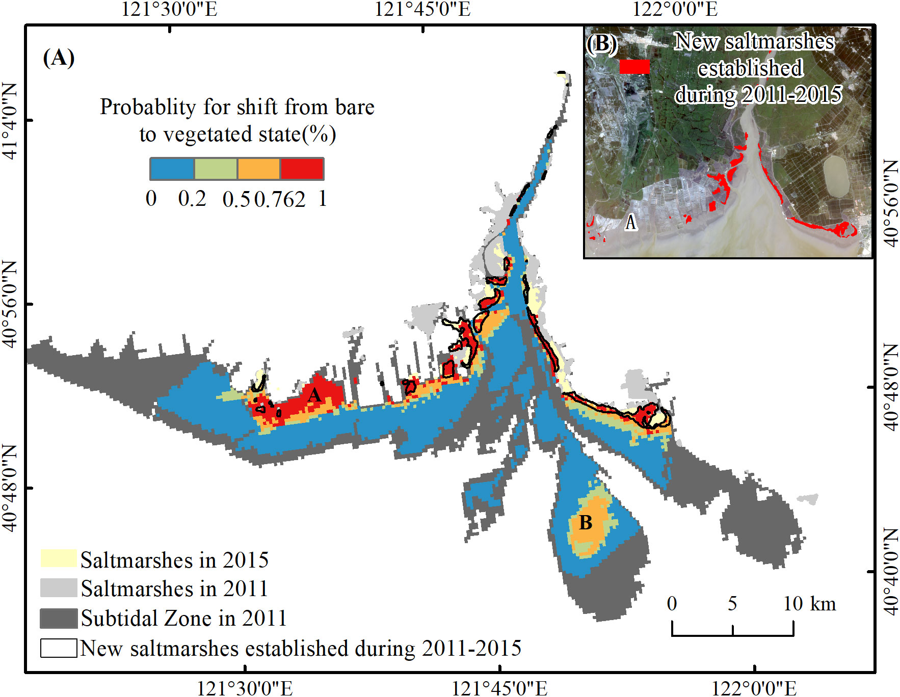
Figure 9 (A) Probability map for a shift from the bare to vegetated state based on the Logistic Regression Model 6. An incorrectly identified area of the new marsh was located in part A. (B) The newly established saltmarshes during 2011-2015 based on the interpretation of remote sensing images which are circled with a black hollow box in (A).

5 Discussion

5.1 The practicability of the topography-driving model in predicting vegetation conversion

Although many external or internal factors have been proposed in predicting the plant colonization of coastal wetlands, the common problem with the prediction was the insufficient information on the integrated response of vegetation to the change in a variety of environmental driving forces (Xiao et al., 2010; Balke et al., 2016). Owing to the coevolution between the ecological and geomorphological components, biogeomorphic modeling takes the advantage of simulating the regime shift from one stable state to another under multiple environmental drivers (D'Alpaos, 2011). Generally in most models, vegetation was considered as a biological driving factor in regulating the evolution of intertidal landforms. For instance, feedbacks between physical and biological processes affect the evolutionary trajectories of saltmarsh ecosystems. The principle was used in a two-dimensional eco-morphodynamic model to predict the response of tidal morphologies to different physical or biological driving scenarios, such as sediment supply, changing sea levels, and colonization by halophytes (D'Alpaos, 2011). Similarly, the evolution of the spatially-averaged elevation in the tidal geomorphological patterns was predicted by the mutual influence of biotic and abiotic components, in which biomass as the product of vegetation cover was one of the driving forces within the Venice lagoon (Marani et al., 2007).

Instead, the topography within the intertidal zone was considered as a determinant factor in shaping the vegetated flats in this paper. The prediction was based on the assumption that past equilibria states of biogeomorphic components drove the establishment of new vegetation. Before the colonization of saltmarshes, the bare flats were controlled by physical feedback. The equilibrium between sedimentation and erosion resulted in the stable state of the low-elevated bare flat. Once the pioneer plants dispersed in the unstable transition zone and opportunistically survived, the positive feedback on the elevation allows the unstable state to evolve into a stable vegetated state. Otherwise, the system was prone to return back to a low-lying bare flat because the seedlings might die out due to their inability to resist the strong hydrodynamic inference or long-term inundation. The positive feedback resulted in not only the expansion of vegetation but also the promotion of elevation. Eventually, a stable state of high-elevation vegetation was expected when the deposition rate came to a halt with reduced inundation(Wang, 2014). In this way, the current vegetation pattern, which reflects the integrated response to past interaction between topography and vegetation will determine future vegetation transformation. When the elevation threshold between the alternative stable states is exceeded, the transition from bare flat to vegetated marshes is predicted to occur (Wang and Temmerman, 2013).

Accordingly, the existence of bimodality in vegetation biomass and elevation was essential for the prediction. Before the simulation, the bimodality was confirmed in the intertidal zone of the Liaohe estuary, which was also demonstrated by Chen (2019). By using the Logistic Regression Model in the front bare flats of Liaohe estuary, the best prediction (R² = 0.739, overall correct percentage =88.6%) for the conversion between the bare flat and vegetation indicated that elevation, combined with slope and elevation change rate contributed the most to vegetation establishment. The conversion rate from bare flat to saltmarsh was up to 3% between 2011 and 2015, which coincided with the investigation that the range of S. salsa was increasing during this period (Wang Y, et al., 2020). Previous research also indicated that geomorphic features not only affect the colonization of seeds but also the growth of seedlings by providing suitable habitats and stable substrates. For instance, specific surface elevation and sufficient flood-free periods were required for seedlings to take root (Friess et al., 2012). In low-elevation areas, waterlogging of depressions under continuous tides often brings about low oxygen stress, which inhibits seedling emergence (Courtwright and Findlay, 2011). Moreover, hydrodynamic stresses, such as waves or tides in the low area can exert dragging or pulling forces on saltmarshes, scouring and eroding sediments near saltmarsh stems and subsurface root systems, and eventually inhibiting early survival of vegetation (Friess et al., 2012). When the elevation threshold was surpassed, the first critical process of the life cycle (“window of opportunity”) occurs (Balke et al., 2014), and thus positive feedback on the elevation increase (Balke et al., 2014; Wang C, et al., 2016).

Besides geomorphic factors, which were effective as explanatory variables in the Logistic Regression Model for predicting vegetation conversion in the Liaohe estuary, other physical factors, including current velocity, and wave velocity, could also be introduced in the model, such as the predicting practice in the Western Scheldt estuary (Wang C, et al., 2020). When the two estuarine wetlands were compared, the intertidal marshes of western Scheldt were more surrounded by subtidal channels and embanked land far from the river mouth (Meire et al., 2005). Instead, the intertidal wetland on shoals along the inlet was closer to land in the Liaohe estuary. Therefore, weighing the driving forces in the different biogeomorphic systems may determine the introduction of specific explanatory variables into the prediction model. The practice attempts in more types of estuarine wetlands will be necessary to evaluate the reliability of the Logistic Regression Model, which allows for some flexibility. The modelling popularization also helps for guiding the restoration and management practice in specific estuarine saltmarshes in the future.

5.2 Factors on the prediction accuracy during the modeling processing

The success of model prediction undoubtedly relies on many objective factors. In this paper, the prediction reliability got benefits from many details during the data processing which is worth consideration. Firstly, the fine DEMs, which were derived from the extracting waterlines, were critical, especially within the unstable state zone. The accuracy during the waterline extraction largely depended on the spatial resolution and timing of multi-temporal satellite images in use before further analysis (Xu et al., 2016; Kang et al., 2017; Tseng et al., 2017). The thresholds for extracting waterlines were based on the Otsu method instead of manual visual validation, thus the positional errors of the waterlines were controlled within one-pixel size (30m for Landsat images) (Liu et al., 2012). However, the fine DEMs in this study was simplified by using the kriging interpolation on the stacking waterlines, which may cause inaccuracy due to the factors such as tide levels, wind, vegetation, topography and so on. In the future in-depth studies, better DEMs with higher accuracy could be considered using intertidal measured bathymetry data, or hydrodynamic models such as Delft3D. The prediction could be improved using DEMs with higher accuracy.

Secondly, the Youden index was verified to promote the prediction accuracy of the Logistic Regression Model. Although 0.5 was generally used in the Logistic Regression Model as the threshold for transformation, the prediction of new marshes, with 0.5 as the threshold in area B (see Figure 9), was inconsistent with the actual conversion. Obviously, the prediction of the stable bare in area B was more convincing with 0.726 (the Youden index) as the threshold, which coincided with the interpretation of the remote image in 2015. However, the large area of new marshes at location A in the prediction (see Figure 9) with 0.5 or 0.726 as the threshold, was inconsistent with the actual conversion. The inaccurate prediction was potentially attributed to human interference. With the increasing development of aquaculture near area A, the vegetation was replaced by mudflat rapidly in the 2000s. Previous research indicated the inflow of polluted water with drugs, fertilizers, and heavy metals, such as Cd, Cu, and Zn into area A triggered the transformation of the original coverage of S. salsa into bare flats before 2011 (Sun, 2018; Yan et al., 2018). The low accessibility of tide in the growth season of S. salsa aggravated the difficulty of vegetation restoration in this area after human interference (Daehler and Strong, 1996). In addition, the strong evaporation in spring associated with the prolonged non-flooding period (>72h) also exacerbated the high soil salinity and inhibited plant colonization or growth (Wang et al., 2010). Therefore, the influence of human activities must have led to the deviation in the prediction results. However, the inconsistent prediction result might help to guide the practice of estuarine restoration in the future.

5.3 Implications of this study for future ecological restoration

To promote effective restoration, a holistic approach is important to predict the biogeomorphic evolution and provide information on early warning locations that have been mostly neglected. When combining the multistability characteristics of intertidal zones and the threshold phenomenon of elevation in coastal wetlands, we successfully predicted the conversion between bare flats and vegetation in the Liaohe estuary. Moreover, the prediction of area A (Figure 9), which was inconsistent with reality, also suggested the restoration priority in the future. Before the restoration work initiates in this area, the impact of geomorphic factors on the saltmarsh settlement should be reassessed from early planning to post-implementation monitoring. In addition, restoration practitioners should weigh the importance of restoring specific ecological functions. Take saltmarsh in area A as an example. It is indisputable that saltmarshes act as essential buffers against the effects of coastal storms, filter nutrients and pollutants from tidal waters, and provide critical habitat for rare and endangered animal species (Möller et al., 2014; Zhang et al., 2021). Therefore, mitigating the external interference on the saltmarsh restoration, such as that of pond aquaculture, should be taken into practice following the topographic reformation. Moreover, the metrics of restored saltmarsh and its associated communities for the desired state must be monitored over time to examine the resistance and resilience capacity.

6 Conclusion

Deep insights into the factors that trigger the shift from the bare flats to vegetated areas are essential for predicting the salt marsh evolution within the intertidal zone. Based on GIS and remote sensing tools, the Logistic Regression Models were applied to predict the regime shift of saltmarshes within the Liaohe estuary. Geomorphic factors, including elevation, slope, and annual change rate in elevation were considered as explanatory variables in determining the vegetation conversion. Based on the prediction, three conclusions were derived as follows. (1) The frequency of pixel elevation and NDVI demonstrate bimodal distribution, confirming two stable states co-exist in the intertidal zone. (2) The highest overall accuracy (88.6%) verified the reliability of the Logistic Regression Model in the prediction of vegetation conversion between 2011 and 2015. The model included elevation, slope, and annual change rate of elevation as variables enhanced the accuracy of prediction in comparison with models that include elevation, slope, or the annual change rate of elevation as variables alone; (3) The predicted area of new mashes in the Liaohe estuary was 16.7km² between 2011 and 2015, mainly located in the seaward front of existing saltmarshes with the conversion rate about 0.8% per year.

Data availability statement

The raw data supporting the conclusions of this article will be made available by the authors, without undue reservation.

Author contributions

XJ: Writing-original draft, data curation, methodology, formal analysis. JY: Conceptualization, supervision, methodology, writing-review & editing, CW: field data collecting, Supervision, methodology, writing-review & editing. BL, HW, and HZ: Funding providing, Review & editing. HYZ and YZ: Funding providing, Data proceeding. All authors contributed to the article and approved the submitted version.

Funding

This research received financial support from the Ministry of Science and Technology of the People’s Republic of China (2022YFC3204302), the China National Administration of Coal Geology (ZMKJ-2021-ZX04), National Key R & D Program of China (2021YFB3901104, 2022YFC330160203), National Nature Science Foundation of China (Grant No. 42006153), Young Elite Scientists Sponsorship Program by CAST (Grant No. 2021QNRC001), the Research Innovation Fund of Tianjin Research Institute for Water Transport Engineering, M.O.T., China (Grant No. TKS20220203), Research for the resources utilization and environmental remediation in coastal zone (ZHTD202106).

Acknowledgments

All claims expressed in this article are solely those of the authors and do not necessarily represent those of their affiliated organizations, or those of the publisher, the editors, and the reviewers. Any product that may be evaluated in this article, or claim that may be made by its manufacturer, is not guaranteed or endorsed by the publisher.

Conflict of interest

The authors declare that the research was conducted in the absence of any commercial or financial relationships that could be construed as a potential conflict of interest.

Publisher’s note

All claims expressed in this article are solely those of the authors and do not necessarily represent those of their affiliated organizations, or those of the publisher, the editors and the reviewers. Any product that may be evaluated in this article, or claim that may be made by its manufacturer, is not guaranteed or endorsed by the publisher.

References

Almeida C. M. R., Mucha A. P., Teresa Vasconcelos M. (2011). Role of different salt marsh plants on metal retention in an urban estuary (Lima estuary, NW Portugal). Estuar. Coast. Shelf Sci. 91 (2), 243–249. doi: 10.1016/j.ecss.2010.10.037

CrossRef Full Text | Google Scholar

Augustin N. H., Cummins R. P., French D. D. (2001). Exploring spatial vegetation dynamics using logistic regression and a multinomial logit model. J. Appl. Ecol. 38, 991–1006. doi: 10.1046/j.1365-2664.2001.00653.x

CrossRef Full Text | Google Scholar

Baier G., Rossi C., Lachaise M., Zhu X. X., Bamler R. (2018). A nonlocal InSAR filter for high-resolution DEM generation from TanDEM-X interferograms. IEEE Trans. Geosci. Remote Sens. 56 (11), 6469–6483. doi: 10.1109/TGRS.2018.2839027

CrossRef Full Text | Google Scholar

Balke T., Herman P. M. J., Bouma T. J., Nilsson C. (2014). Critical transitions in disturbance-driven ecosystems: identifying windows of opportunity for recovery. J. Ecol. 102 (3), 700–708. doi: 10.1111/1365-2745.12241

CrossRef Full Text | Google Scholar

Balke T., Stock M., Jensen K., Bouma T. J., Kleyer M. (2016). A global analysis of the seaward salt marsh extent: The importance of tidal range. Water Resour. Res. 52 (5), 3775–3786. doi: 10.1002/2015WR018318

CrossRef Full Text | Google Scholar

Baustian J. J., Mendelssohn I. A., Hester M. W. (2012). Vegetation's importance in regulating surface elevation in a coastal salt marsh facing elevated rates of sea level rise. Global Change Biol. 18 (11), 3377–3382. doi: 10.1111/j.1365-2486.2012.02792.x

CrossRef Full Text | Google Scholar

Blott S. J., Pye K. (2004). Application of lidar digital terrain modeling to predict intertidal habitat development at a managed retreat site: Abbotts hall, Essex, UK. Earth Surf. Process. Landf. 29 (7), 893–905. doi: 10.1002/esp.1082

CrossRef Full Text | Google Scholar

Bouma T., Vries M. D., Low E., Kusters L., Herman P., Tanczos I., et al. (2005). Flow hydrodynamics on a mudflat and in salt marsh vegetation: identifying general relationships for habitat characterisations. Hydrobiologia. 540, 259–274. doi: 10.1007/s10750-004-7149-0

CrossRef Full Text | Google Scholar

Calef M. P., David McGuire A., Epstein H. E., Scott Rupp T., Shugart H. H. (2005). Analysis of vegetation distribution in interior Alaska and sensitivity to climate change using a logistic regression approach. J. Biogeogr. 32 (5), 863–878. doi: 10.1111/j.1365-2699.2004.01185.x

CrossRef Full Text | Google Scholar

Cao C., Su F., Song F., Yan H., Pang Q. (2022). Distribution and disturbance dynamics of habitats suitable for suaeda salsa. Ecol. Indic. 140, 108984. doi: 10.1016/j.ecolind.2022.108984

CrossRef Full Text | Google Scholar

Catry F. X., Rego F. C., Bação F. L., Moreira F. (2009). Modeling and mapping wildfire ignition risk in Portugal. Int. J. Wildland Fire. 18 (8), 921–931. doi: 10.1071/WF07123

CrossRef Full Text | Google Scholar

Chang Y., Zhu Z., Bu R., Chen H., Feng Y., Li Y., et al. (2013). Predicting fire occurrence patterns with logistic regression in heilongjiang province, China. Landsc. Ecol. 28 (10), 1989–2004. doi: 10.1007/s10980-013-9935-4

CrossRef Full Text | Google Scholar

Chen L. (2019). Bistability of intertidal ecosystems in Liaohe estuary based on GIS and RS. [master's thesis] (Jingzhou, China: Yangtze University).

Google Scholar

Costanza R., d'Arge R., De Groot R., Farber S., Grasso M., Hannon B., et al. (1997). The value of the world's ecosystem services and natural capital. nature 387 (6630), 253–260.

Google Scholar

Courtwright J., Findlay S. E. (2011). Effects of microtopography on hydrology, physicochemistry, and vegetation in a tidal swamp of the Hudson river. Wetlands. 31, 239–249. doi: 10.1007/s13157-011-0156-9

CrossRef Full Text | Google Scholar

D'Alpaos A. (2011). The mutual influence of biotic and abiotic components on the long-term ecomorphodynamic evolution of salt-marsh ecosystems. Geomorphology. 126 (3-4), 269–278. doi: 10.1016/j.geomorph.2010.04.027

CrossRef Full Text | Google Scholar

D'Alpaos A., Lanzoni S., Marani M., Rinaldo A. (2007). Landscape evolution in tidal embayments: Modeling the interplay of erosion, sedimentation, and vegetation dynamics. J. Geophys. Res. 112:1–17. doi: 10.1029/2006jf000537

CrossRef Full Text | Google Scholar

Daehler C. C., Strong D. R. (1996). Status, prediction and prevention of introduced cordgrass spartina spp invasions in pacific estuaries, USA. Biol. Conserv. 78 (1-2), 51–58. doi: 10.1016/0006-3207(96)00017-1

CrossRef Full Text | Google Scholar

Davy A. J., Brown M. J., Mossman H. L., Grant A. (2011). Colonization of a newly developing salt marsh: disentangling independent effects of elevation and redox potential on halophytes. J. Ecol. 99 (6), 1350–1357. doi: 10.1111/j.1365-2745.2011.01870

CrossRef Full Text | Google Scholar

Friess D. A., Krauss K. W., Horstman E. M., Balke T., Bouma T. J., Galli D., et al. (2012). Are all intertidal wetlands naturally created equal? bottlenecks, thresholds and knowledge gaps to mangrove and saltmarsh ecosystems. Biol. Rev. 87 (2), 346–366. doi: 10.1111/j.1469-185X.2011.00198.x

CrossRef Full Text | Google Scholar

Garcia C. V., Woodard P., Titus S., Adamowicz W., Lee B. (1995). A logit model for predicting the daily occurrence of human caused forest-fires. Int. J. Wildland Fire. 5 (2), 101–111. doi: 10.1071/WF9950101

CrossRef Full Text | Google Scholar

Ge Z., Cao H., Zhang L. (2013). A process-based grid model for the simulation of range expansion of spartina alterniflora on the coastal saltmarshes in the Yangtze estuary. Ecol. Engineering. 58, 105–112. doi: 10.1016/j.ecoleng.2013.06.024

CrossRef Full Text | Google Scholar

Gu J., Luo M., Zhang X., Christakos G., Agusti S., Duarte C. M., et al. (2018). Losses of salt marsh in China: Trends, threats and management. Estuar. Coast. Shelf Sci. 214, 98–109. doi: 10.1016/j.ecss.2018.09.015

CrossRef Full Text | Google Scholar

Guo Q., Li W., Yu H., Alvarez O. (2010). Effects of topographic variability and lidar sampling density on several DEM interpolation methods. Photogramm. Eng. Remote Sens. 76 (6), 701–712. doi: 10.14358/PERS.76.6.701

CrossRef Full Text | Google Scholar

Heygster G., Dannenberg J., Notholt J. (2010). Topographic mapping of the German tidal flats analyzing SAR images with the waterline method. IEEE Trans. Geosci. Remote Sensing. 48 (3), 1019–1030. doi: 10.1109/tgrs.2009.2031843

CrossRef Full Text | Google Scholar

Hu Z., Xu Y., Yin Y., Zhang K., Wu G., Wang C., et al. (2021). Tidal flats dataset covers coastal region in north of 18°N latitude of China, (1989-2020). J. Glob. Change. Data. Discovery 6 (1), 125–132. doi: 10.3974/geodb.2021.10.06.V1

CrossRef Full Text | Google Scholar

Huang H., Zhang L., Guan Y., Wang D. (2008). A cellular automata model for population expansion of spartina alterniflora at jiuduansha shoals, shanghai, China. Estuar. Coast. Shelf Sci. 77 (1), 47–55. doi: 10.1016/j.ecss.2007.09.003

CrossRef Full Text | Google Scholar

Jiménez-Valverde A. (2012). Insights into the area under the receiver operating characteristic curve (AUC) as a discrimination measure in species distribution modeling. Glob. Ecol. Biogeogr. 21 (4), 498–507. doi: 10.1111/j.1466-8238.2011.00683.x

CrossRef Full Text | Google Scholar

Kang Y., Ding X., Xu F., Zhang C., Ge X. (2017). Topographic mapping on large-scale tidal flats with an iterative approach on the waterline method. Estuar. Coast. Shelf Sci. 190, 11–22. doi: 10.1016/j.ecss.2017.03.024

CrossRef Full Text | Google Scholar

Karstens S., Jurasinski G., Glatzel S., Buczko U. (2016). Dynamics of surface elevation and microtopography in different zones of a coastal phragmites wetland. Ecol. Eng. 94, 152–163. doi: 10.1016/j.ecoleng.2016.05.049

CrossRef Full Text | Google Scholar

Kim J. H., Fourcaud T., Jourdan C., Maeght J., Mao Z., Metayer J., et al. (2017). Vegetation as a driver of temporal variations in slope stability: The impact of hydrological processes. Geophys. Res. Lett. 44 (10), 4897–4907. doi: 10.1002/2017gl073174

CrossRef Full Text | Google Scholar

Lang Y., Wang N., Gao H., Bai J. (2012). Distribution and risk assessment of polycyclic aromatic hydrocarbons (PAHs) from liaohe estuarine wetland soils. Environ. Monit Assess. 184 (9), 5545–5552. doi: 10.1007/s10661-011-2360-8

PubMed Abstract | CrossRef Full Text | Google Scholar

Li G., Lang Y., Yang W., Peng P., Wang X. (2014). Source contributions of PAHs and toxicity in reed wetland soils of liaohe estuary using a CMB–TEQ method. Sci. Total Environ. 490, 199–204. doi: 10.1016/j.scitotenv.2014.05.001

PubMed Abstract | CrossRef Full Text | Google Scholar

Li H., Li L., Su F., Wang T., Gao P. (2021). Ecological stability evaluation of tidal flat in coastal estuary: A case study of liaohe estuary wetland, China. Ecol. Indic. 130 (108), 32–42. doi: 10.1016/j.ecolind.2021.108032

CrossRef Full Text | Google Scholar

Liu Y., Li M., Cheng L., Li F., Chen K. (2012). Topographic mapping of offshore sandbank tidal flats using the waterline detection method: A case study on the dongsha sandbank of jiangsu radial tidal sand ridges, China. Mar. Geod. 35 (4), 362–378. doi: 10.1080/01490419.2012.699501

CrossRef Full Text | Google Scholar

Marani M., D'Alpaos A., Lanzoni S., Carniello L., Rinaldo A. (2007). Biologically‐controlled multiple equilibria of tidal landforms and the fate of the Venice lagoon. Geophys. Res. Lett. 34 (11), L11402. doi: 10.1029/2007GL030178

CrossRef Full Text | Google Scholar

Meire P., Ysebaert T., Damme S. V., Bergh E., Maris T., Struyf E. (2005). The scheldt estuary: a description of a changing ecosystem. Hydrobiologia. 540 (1), 1–11. doi: 10.1007/s10750-005-0896-8

CrossRef Full Text | Google Scholar

Moeslund J. E., Arge L., Bøcher P. K., Dalgaard T., Odgaard M. V., Nygaard B., et al. (2013). Topographically controlled soil moisture is the primary driver of local vegetation patterns across a lowland region. Ecosphere. 4 (7), 1–26. doi: 10.1890/ES13-00134.1

CrossRef Full Text | Google Scholar

Möller I., Kudella M., Rupprecht F., Spencer T., Paul M., van Wesenbeeck B. K., et al. (2014). Wave attenuation over coastal salt marshes under storm surge conditions. Nat. Geosci. 7 (10), 727–731. doi: 10.1038/ngeo2251

CrossRef Full Text | Google Scholar

Otsu N. (1979). A threshold selection methodfrom Gray-level histograms. IEEE Trans. Syst. Man Cybern. Syst. 9 (1), 62–66. Available at: https://cw.fel.cvut.cz/b201/_media/courses/a6m33bio/otsu.pdf

Google Scholar

Pennings S. C., Callaway R. M. (1992). Salt marsh plant zonation: the relative importance of competition and physical factors. Ecology 73 (2), 681–690. doi: 10.2307/1940774

CrossRef Full Text | Google Scholar

Ryu J.-H., Kim C.-H., Lee Y.-K., Won J.-S., Chun S.-S., Lee S. (2008). Detecting the intertidal morphologic change using satellite data. Estuarine Coast. Shelf Sci. 78 (4), 623–632. doi: 10.1016/j.ecss.2008.01.020

CrossRef Full Text | Google Scholar

Ryu J.-H., Won J.-S., Min K.D.J.R. (2002). Waterline extraction from landsat TM data in a tidal flat: a case study in gomso bay, Korea. Remote Sens. Environment. 83 (3), 442–456. doi: 10.1016/S0034-4257(02)00059-7

CrossRef Full Text | Google Scholar

Sagar S., Roberts D., Bala B., Lymburner L. (2017). Extracting the intertidal extent and topography of the Australian coastline from a 28 year time series of landsat observations. Remote Sens Environ. 195, 153–169. doi: 10.1016/j.rse.2017.04.009

CrossRef Full Text | Google Scholar

Scheffer M., Carpenter S. R. (2003). Catastrophic regime shifts in ecosystems: linking theory to observation. Trends Ecol. Evol. 18 (12), 648–656. doi: 10.1016/j.tree.2003.09.002

CrossRef Full Text | Google Scholar

Scott D. B., Frail-Gauthier J., Mudie P. J. (2014). Coastal wetlands of the world: geology, ecology, distribution and applications (Cambridge: Cambridge University Press).

Google Scholar

Stark J., Van Oyen T., Meire P., Temmerman S. (2015). Observations of tidal and storm surge attenuation in a large tidal marsh. Limnol. Oceanogr. 60 (4), 1371–1381. doi: 10.1002/lno.10104

CrossRef Full Text | Google Scholar

Sun Z. (2018). Interannual change of Suaeda heteroptera in the wetland of Liaohe Estuary andcorrelation study of its influencing factors. master's thesis (China Dalian: Dalian Ocean University).

Google Scholar

Tong S. S., Deroin J. P., Pham T. L. (2020). An optimal waterline approach for studying tidal flat morphological changes using remote sensing data: A case of the northern coast of Vietnam. Estuar. Coast. Shelf Sci. 236, 106613. doi: 10.1016/j.ecss.2020.106613

PubMed Abstract | CrossRef Full Text | Google Scholar

Tseng K.-H., Kuo C.-Y., Lin T.-H., Huang Z.-C., Lin Y.-C., Liao W.-H., et al. (2017). Reconstruction of time-varying tidal flat topography using optical remote sensing imageries. ISPRS-J. Photogramm. Remote Sens. 131, 92–103. doi: 10.1016/j.isprsjprs.2017.07.008

CrossRef Full Text | Google Scholar

van Belzen J., van de Koppel J., Kirwan M. L., van der Wal D., Herman P. M. J., Dakos V., et al. (2017). Vegetation recovery in tidal marshes reveals critical slowing down under increased inundation. Nat. Commun. 8 (1), 15811. doi: 10.1038/ncomms15811

PubMed Abstract | CrossRef Full Text | Google Scholar

Vilar del Hoyo L., Martín Isabel M. P., Martínez Vega F. J. (2011). Logistic regression models for human-caused wildfire risk estimation: analysing the effect of the spatial accuracy in fire occurrence data. Eur. J. For. Res. 130 (6), 983–996. doi: 10.1007/s10342-011-0488-2

CrossRef Full Text | Google Scholar

Wang C. (2014). Biogeomorphic regime shifts between vegetated and bare states in tidal wetlands. [doctor's thesis] (Antwerpen, Belgium: University of Antwerpen).

Google Scholar

Wang Y., Ji Y., Sun Z., Li J., Zhang M., Wu G. (2020). “Analysis of suaeda heteroptera cover change and its hydrology driving factors in the liao river estuary wetlands, China,” in IOP Conference Series: Earth and Environmental Science (IOP Publishing). 467(1), 012150 doi: 10.1088/1755-1315/467/1/012150

CrossRef Full Text | Google Scholar

Wang Y., Liu R., Gao H., Bai J., Ling M. (2010). Degeneration mechanism research of suaeda heteroptera wetland of the shuangtaizi estuary national nature reserve in China. Proc. Environ. Sci. 2, 1157–1162. doi: 10.1016/j.proenv.2010.10.124

CrossRef Full Text | Google Scholar

Wang C., Smolders S., Callaghan D. P., van Belzen J., Bouma T. J., Hu Z., et al. (2020). Identifying hydro-geomorphological conditions for state shifts from bare tidal flats to vegetated tidal marshes. Remote Sens. 12 (14). doi: 10.3390/rs12142316

CrossRef Full Text | Google Scholar

Wang C., Temmerman S. (2013). Does biogeomorphic feedback lead to abrupt shifts between alternative landscape states?: an empirical study on intertidal flats and marshes. J. Geophys. Res.-Earth Surf. 118 (1), 229–240. doi: 10.1029/2012JF002474

CrossRef Full Text | Google Scholar

Wang G., Wang M., Jiang M., Lyu X., He X., Wu H. (2017). Effects of vegetation type on surface elevation change in liaohe river delta wetlands facing accelerated sea level rise. Chin. Geogr. Sci. 27 (5), 810–817. doi: 10.1007/s11769-017-0909-3

CrossRef Full Text | Google Scholar

Wang G., Wang M., Lu X., Jiang M. (2016). Surface elevation change and susceptibility of coastal wetlands to sea level rise in liaohe delta, China. Estuar. Coast. Shelf Sci. 180, 204–211. doi: 10.1016/j.ecss.2016.07.011

CrossRef Full Text | Google Scholar

Wang C., Wang Q., Meire D., Ma W., Wu C., Meng Z., et al. (2016). Biogeomorphic feedback between plant growth and flooding causes alternative stable states in an experimental floodplain. Adv Water Resour 93, 223–235. doi: 10.1016/j.advwatres.2015.07.003

CrossRef Full Text | Google Scholar

Xiao D., Li X. (2004). “Ecological and environmental function of wetland landscape in the Liaohe Delta,” in Wetlands ecosystems in Asia (Shenyang, Elsevier), 35–46.

Google Scholar

Xiao D. R., Zhang L. Q., Zhu Z. C. (2010). The range expansion patterns of spartina alterniflora on salt marshes in the Yangtze estuary, China. Estuar. Coast. Shelf Sci. 88 (1), 99–104. doi: 10.1016/j.ecss.2010.03.015

CrossRef Full Text | Google Scholar

Xie T., Cui B., Li S., Bai J. (2019). Topography regulates edaphic suitability for seedling establishment associated with tidal elevation in coastal salt marshes. Geoderma. 337, 1258–1266. doi: 10.1016/j.geoderma.2018.07.053

CrossRef Full Text | Google Scholar

Xie T., Wang Q., Ning Z., Chen C., Cui B., Bai J., et al. (2021). Artificial modification on lateral hydrological connectivity promotes range expansion of invasive spartina alterniflora in salt marshes of the yellow river delta, China. Sci. Total Environ. 769, 144476. doi: 10.1016/j.scitotenv.2020.144476

PubMed Abstract | CrossRef Full Text | Google Scholar

Xu H. (2007). Modification of normalised difference water index (NDWI) to enhance open water features in remotely sensed imagery. Int. J. Remote Sens. 27 (14), 3025–3033. doi: 10.1080/01431160600589179

CrossRef Full Text | Google Scholar

Xu Z., Kim D.-j., Kim S. H., Cho Y.-K., Lee S.-G. (2016). Estimation of seasonal topographic variation in tidal flats using waterline method: A case study in gomso and hampyeong bay, south Korea. Estuar. Coast. Shelf Sci. 183, 213–220. doi: 10.1016/j.ecss.2016.10.026

CrossRef Full Text | Google Scholar

Yan X., Liu M., Zhong J., Guo J., Wu W. (2018). How human activities affect heavy metal contamination of soil and sediment in a long-term reclaimed area of the liaohe river delta, north China. Sustainability. 10 (2), 338. doi: 10.3390/su10020338

CrossRef Full Text | Google Scholar

Yong Z., Dong Z., Huili D., Nan X., Huiming Z., Xin H., et al. (2021). The enhanced construction method for intertidal terrain of offshore sandbanks by remote sensing. J. Oceanogr. 43 (12), 133–143. doi: 10.12284/hyxb2021

CrossRef Full Text | Google Scholar

Yu Z., Gao J., Wu X. (1989). Difference between mean sea level and national geoid(1985)along the coast of china. J. Oceanogr. Taiwan strait 8 (2), 97–104.

Google Scholar

Zhang J., Bai Y., Huang Z., Zhang Z., Li D. (2021). Community composition and behavioral differences of migrating shorebirds between two habitats within a suaeda salsa saltmarsh-mudflat wetland mosaics. Biodivers. Sci. 29 (3), 351. doi: 10.17520/biods.2020189

CrossRef Full Text | Google Scholar

Zhao B., Guo H., Yan Y., Wang Q., Li B. (2008). A simple waterline approach for tidelands using multi-temporal satellite images: a case study in the Yangtze delta. Estuarine Coast. Shelf Sci. 77 (1), 134–142. doi: 10.1016/j.ecss.2007.09.022

CrossRef Full Text | Google Scholar

Zhu L., Wu J., Xu Y., Hu R., Wang N. (2010). Recent geomorphic changes in the liaohe estuary. J. Geogr. Sci. 20 (1), 31–48. doi: 10.1007/s11442-010-0031-2

CrossRef Full Text | Google Scholar