Application of a Robin boundary condition to surface waves

1 Introduction

We study surface gravity waves in a homogeneous ocean where the depth is very much larger than the wavelength. These waves are affected by the physical conditions at the sea surface, most notably by the presence of thin flexible covers like biogenic films, which may cover large areas of the ocean surface (Gade et al., 2006). In addition to these natural films, we find pollutant slicks from petroleum spills or municipal effluents, which change the surface conditions. In cold regions, the surface cover is usually related to the presence of ice, for example, grease ice (Martin and Kauffman, 1981; Sutherland et al., 2019), or densely packed ice rubble in the marginal ice zone (Squire, 1984). Another example is the seasonal accumulation of Sargassum mats in the Tropical Atlantic (Marsh et al., 2022).

It is practically impossible to formulate a unified mathematical theory for explaining the effect on surface waves of floating material like oil, grease ice, or vegetation. We therefore intend to model this interaction by introducing a freely varying parameter R, which can be adapted to the problem in question. This parameter appears in a very general condition at the ocean surface. The condition is called a Robin condition (Gustafson, 1998; Akin, 2005) and R is the Robin parameter. Traditionally, the Robin condition is a relation between a quantity T (temperature, velocity, etc.) and its derivative $\partial T/\partial x_n$, where $x_n$ is directed normal to the boundary. The homogeneous Robin condition can be written $\partial T/\partial x_n+RT=0$ at the boundary (sometimes $\widehat{R}\partial T/\partial x_n+T=0$ is used). In this way, the Robin condition becomes a weighted combination of Dirichlet and Neumann boundary conditions. It is common in many branches of physics; see, for example, Hahn and Ozisk (2012) for applications to heat conduction, Tyvand and Nøland (2019) for convection in a porous medium, and Weber and Børve (2021) in the case of continental shelf waves with a permeable coastline. The relevance for oceanographic purposes is the role of the fluctuating tangential stress at the surface, which is typically small compared to the fluctuating normal stress (form stress) for uncontaminated surfaces, but can be large when the surface is covered by sea slicks, oil spills, sea ice, and other materials (e.g., Dorrestein, 1951). The framework presented here is mostly relevant for waves in deep water since the bottom friction and wave radiation stresses will typically dominate in shallow water. We will therefore only discuss waves for which $kH\gg 1$, where k is the wave number and H is the local water depth. We will also ignore rotational effects; hence, we assume that $\omega \gg f$, where $\omega$ is the angular frequency of the waves and f is the Coriolis parameter.

In Figure 1, we have depicted a general configuration relevant to the discussion here. The x-axis is horizontal and placed along the undisturbed sea surface, while the z-axis is positive upwards. The x-direction is, without loss of generality, in the direction of wave propagation. In the presence of waves, the sea surface is given by $z=\eta (x,y,t)$.

FIGURE 1

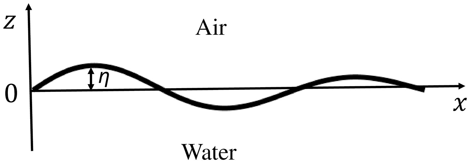
Figure 1 A diagram of spatially damped surface waves. The surface can be free or covered by a flexible layer, depending on the problem in question.

We shall here use the Robin formalism to describe the tangential conditions at the surface. Thus, we write

$\begin{array}{ll}\partial u/\partial z+\partial w/\partial x+Ru=0, z=\eta (x,y,t),& (1)\end{array}$

where u and w are the horizontal and vertical velocity components. In Equation 1, R is generally complex, i.e.,

$\begin{array}{ll}R=R_r+i{R}_i.& (2)\end{array}$

We note from Equation 1 that when $R=0$, the viscous shear stress at the surface vanishes, defining a free surface. At the other extreme, when $R\to \infty$, the horizontal motion is zero at the surface, which models a flexible, but horizontally inextensible top layer (Lamb, 1932). The application of Equation 1 as a general model for the physical conditions at the surface appears to be novel. We will relate the Robin parameter to the rate of growth and decay in the waves, using known examples for elastic monolayers and thin layers of viscous fluids to aid the physical interpretation of our results.

The rest of this paper is organized as follows: In Section 2, we calculate the wave attenuation/growth by applying the Robin condition, and in Section 3, we discuss the solution when the Robin parameter is purely real. The case of a complex Robin parameter is considered in Section 4. Energy considerations due to dilational waves excited in the surface layer is discussed in Section 5. Finally, Section 6 contains some concluding remarks.

2 Mathematical analysis

We here consider two-dimensional wave motion in a viscous ocean. For a fluid with viscosity ν, the two-dimensional velocity field can be separated into two parts: one potential part $\phi$ and one vorticity part $\psi$; see Lamb (1932), such that

$\begin{array}{ll}u=-\partial \phi /\partial x-\partial \psi /\partial \mathrm{z,}& (3)\end{array}$

$\begin{array}{ll}w=-\partial \phi /\partial z+\partial \psi /\partial \mathrm{x.}& (4)\end{array}$

Inserting into the governing equations, we then obtain for the linear part of the wave field

$\begin{array}{ll}{\partial }^2\phi /\partial x^2+{\partial }^2\phi /\partial z^2=\mathrm{0,}& (5)\end{array}$

$\begin{array}{ll}\partial \psi /\partial t-\nu ({\partial }^2\psi /\partial x^2+{\partial }^2\psi /\partial z^2)=\mathrm{0,}& (6)\end{array}$

$\begin{array}{ll}p/\rho =\partial \phi /\partial t-gz.& (7)\end{array}$

Assuming that $\phi ,\psi \to 0, z\to -\infty$, the normalized linear solutions can be written

$\begin{array}{ll}\phi =\exp (\kappa z)\exp i(\kappa x-nt),& (8)\end{array}$

$\begin{array}{ll}\psi =C\exp (mz)\exp i(\kappa x-nt),& (9)\end{array}$

where C is a constant. In Equations 8 and 9, the complex wave number and frequency are defined by

$\begin{array}{ll}\kappa =k+i\alpha ,& (10)\end{array}$

$\begin{array}{ll}n=\omega -i\beta .& (11)\end{array}$

Here $\alpha$,$\beta$ are the real (and small) spatial and temporal damping rates. From Equation 6, we obtain that $m^2={\kappa }^2-in/\nu$. If we now assume that the wavelength is much larger than the thickness of the oscillatory viscous boundary layer, and that the wave growth/damping is slow compared to the wave period, we have $\left|m\right|\gg \left|\kappa \right|$ and $|\omega \gg \left|\beta \right|$. Then, we have to leading order that

$\begin{array}{ll}m=(1-i)\mathrm{\gamma ,}& (12)\end{array}$

where $\gamma$ is defined by

$\begin{array}{ll}\gamma ={\omega }^{1/2}/{(2\nu )}^{1/2}.& (13)\end{array}$

Here, the quantity ${\gamma }^{-1}$ represents the thin viscous boundary-layer thickness at the surface. To obtain Equation 12, we thus assume that $k/\gamma \ll 1.$ From Equation 1, we find that

$\begin{array}{ll}C=-i\kappa (2\kappa +R)/(m^2+mR+{\kappa }^2).& (14)\end{array}$

Finally, assuming no fluctuating normal stress at the water surface, the dynamic boundary condition in the z-direction becomes

$\begin{array}{ll}p/\rho =2\nu \partial w/\partial z\text{,\hspace{0.17em}}z=\mathit{\eta .}& (15)\end{array}$

It is worth noting at this point that capillary waves can be included in the analysis by adding the normal stress due to the equilibrium value of the surface tension in Equation 15; see, for example, Lucassen (1968). The main conclusions in the present study will not change, however, and we ignore capillary waves in our examples here since their inclusion complicates the mathematical expressions without contributing to the physical interpretation of our results. From Equation 15, we find that

$\begin{array}{ll}\eta =(1/g)[(-in+2\nu {\kappa }^2)\phi -2i\kappa m\psi ],z=0& (16)\end{array}$

Inserting from Equations 8 and 9 into Equation 16, we obtain the dispersion relation for this problem:

$\begin{array}{ll}{n}^2+2i\nu {\kappa }^{2}n-g\kappa +iM=\mathrm{0,}& (17)\end{array}$

where

$\begin{array}{ll}M=-{\kappa }^2(ig+2\nu mn)(2\kappa +R)/(m^2+mR+{\kappa }^2).& (18)\end{array}$

Utilizing Equations 10–12, we obtain from the real part of Equation 17 to lowest order the obvious result ${\omega }^2=gk$. The imaginary part yields to lowest order that

$\begin{array}{ll}\beta +c_g\alpha =\omega k^2/(2{\gamma }^2)+\Re (M)/(2\omega ),& (19)\end{array}$

where now $c_g=\omega /(2k)$ is the usual deep-water wave group velocity. Here, $\Re$ denotes the real part of a complex quantity. We define a nondimensional Robin parameter by

$\begin{array}{ll}A=R_r/\gamma ,B=R_i/\gamma & (20)\end{array}$

and we scale $\beta$ in Equation 19 by ${\beta }_{inex}=\omega k/(4\gamma )$, which is the temporal damping coefficient for an inextensible surface film (Lamb, 1932). Furthermore, we define $\widehat{\beta }=\beta /{\beta }_{inex}$ and the nondimensional spatial damping rate by $\widehat{\alpha }=4\gamma \alpha /k^2$. Using that $k/\gamma \ll 1, \beta /\omega \ll 1$, and $\alpha /k\ll 1$, we obtain from Equation 19 that

$\begin{array}{ll}\widehat{\beta }+\frac{1}{2}\widehat{\alpha }=(2k/\gamma )P+Q,& (21)\end{array}$

where

$\begin{array}{ll}P=1+2/[A^2+B^2+2A-2B+2],& (22)\end{array}$

$\begin{array}{ll}Q=(A^2+B^2+2A)/[A^2+B^2+2A-2B+2].& (23)\end{array}$

In Equations 22 and 23, $A,B\in (-\infty ,\infty )$, and it is easily seen that both P and Q are of order unity. When $A=B=0$, we have $P=2$ and $Q=0$. Then Equation 21, in dimensional form, reduces to $\beta +c_g\alpha =\omega k^2/{\gamma }^2$, as first obtained in Jenkins (1986) for a free surface. For larger values of A, B, we find that $(2k/\gamma )P$ becomes negligible in Equation 20. A general form of Equation 19 for damped waves has been derived in Weber (2022), relating the right-hand side to the dissipation in the wave motion.

3 Real Robin parameter

It is natural to start our discussion for the case when R is purely real, i.e., when $B=0$ in Equations 22 and 23. In Figure 2, we have plotted the attenuation rate $Q$ vs. $A=R_r/\gamma$ in this case. We will assume that the waves are already present; hence, we ignore the generation mechanism and focus on the transient development of the existing wave field. In our analysis here, it is the fluctuating part of the tangential surface stress that is of interest, and hence, we will neglect the slowly varying wind stress that contributes to the upper ocean Ekman response, which is a second-order effect in the theoretical framework we apply here (e.g., Weber, 1983).

FIGURE 2

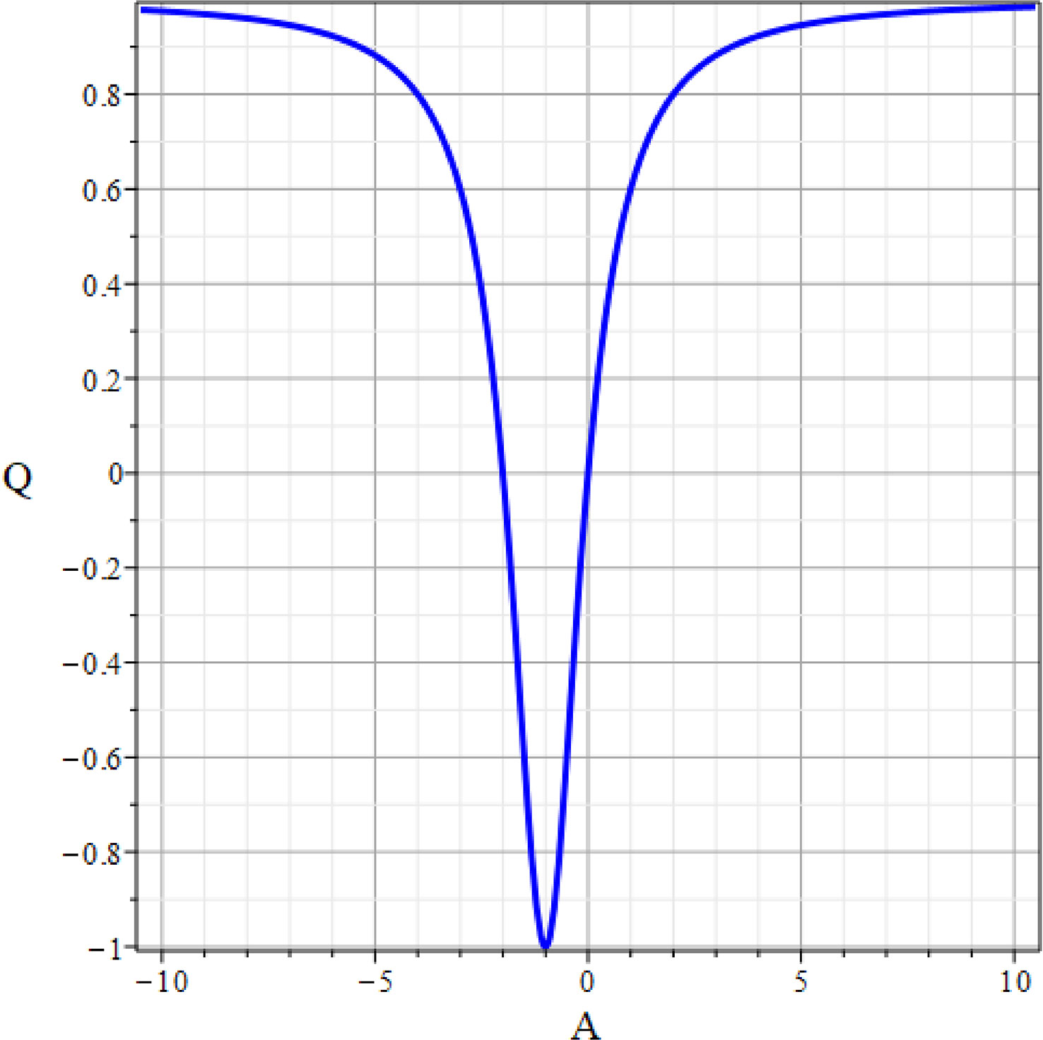
Figure 2 Nondimensional attenuation rate $Q$ from (22) for deep-water waves as a function of the nondimensional real Robin parameter $A=R_r/\gamma$.

We note from Figure 2 that the depicted line tends to unity as $A$ becomes infinitely large. Physically, this means that the horizontal velocity becomes zero at the contact with the surface cover, which is often referred to as the inextensible layer limit. Overall, real $R$ is related to wave damping $(Q>0)$. However, it is interesting to note that $Q<0$ (wave growth) occurs when $-2\le A\le 0$. This may be explained in terms of the wave energy balance. From Equation 1, we may write at the surface that

$\begin{array}{ll}\rho \nu (\partial u/\partial z+\partial w/\partial x)=\tau =-\rho \nu Ru,& (24)\end{array}$

where $\tau$ is the horizontal shear stress at the surface. Hence, by multiplying with the real $u$ and average over the wave cycle (denoted by an over-bar), we find for the work per unit time of the shear stress on the fluid that

$\begin{array}{ll}\overline{\tau u}=-\rho \nu R\overline{u^2}, z=0.& (25)\end{array}$

We note that the work is proportional to the square of the horizontal velocity component and independent of the vertical velocity. This is a general result that holds for any value of the Robin parameter. From Equation 25, we realize that to have a positive energy input, we must have $R<0.$ Furthermore, to have wave growth, this input must be larger than the viscous dissipation $D$ in the fluid. Here,

$\begin{array}{ll}D=\rho \nu \underset{-\infty }{\overset{0}{\int }}(\overline{\nabla u·\nabla u}+\overline{\nabla w·\nabla w})dz& (26)\end{array}$

Due to the strong gradients near the surface, $\overline{{(\partial u/\partial z)}^2}$ will dominate in Equation 26. We derive real velocities from Equations 2, 3, 8, 9, and 14, and use that $k/\gamma \ll 1$. In Figure 3, we have plotted the dimensionless quantities $f_1=2\overline{\tau u}/(\rho \nu k^2\gamma )$ and $f_2=2D/(\rho \nu k^2\gamma )$ as functions of $A$.

FIGURE 3

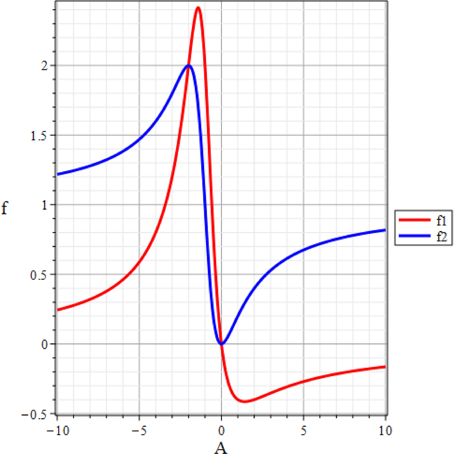
Figure 3 Work by the dimensionless surface stress ($f_1)$ and the dimensionless dissipation ($f_2)$ as functions of the nondimensional real Robin parameter $A=R_r/\gamma$.

We note that in a small window, $-2\le A\le 0$, the work by the surface stress is larger than the dissipation, so here we have wave growth. The maximum growth occurs for $A=-1$. At $A=-2$, the two effects balance, so here the growth rate is zero. These results confirm the findings for the attenuation rates depicted in Figure 2.

Jenkins and Jacobs (1997) studied the wave damping by a thin layer of viscous fluid on top of an infinitely deep fluid of a different viscosity. For a thin, very viscous film of thickness$d$, they showed that the dynamic boundary condition in the horizontal direction between the two immiscible fluids could be written as

$\begin{array}{ll}\partial u/\partial z+\partial w/\partial x+(4d{k}^2{\mu }_s/\mu )u=0, z=0& (27)\end{array}$

where ${\mu }_s$ and $\mu$ are the dynamic viscosities of the thin upper surface layer and the infinitely deep bottom layer, respectively. Now, by comparison with Equation 1, we see that in this case

$\begin{array}{ll}{R}_r=4d{k}^2{\mu }_s/\mu ,& (28)\end{array}$

$\begin{array}{ll}{R}_i=0.& (29)\end{array}$

Since $R$ is purely real, the damping in this case will follow the curve for $A>0$in Figure 2. Here, we ignore any internal motion in the film itself since the analysis is only valid for thin films, with monomolecular films as the limit.

4 Damping for a complex Robin parameter

We now study the case $R_r=\gamma A\ge 0, R_i=\gamma B\ge 0$. In Figure 4, we have plotted the attenuation rate $Q$ from Equation 23 as a function of $B$ for various values of $A$.

FIGURE 4

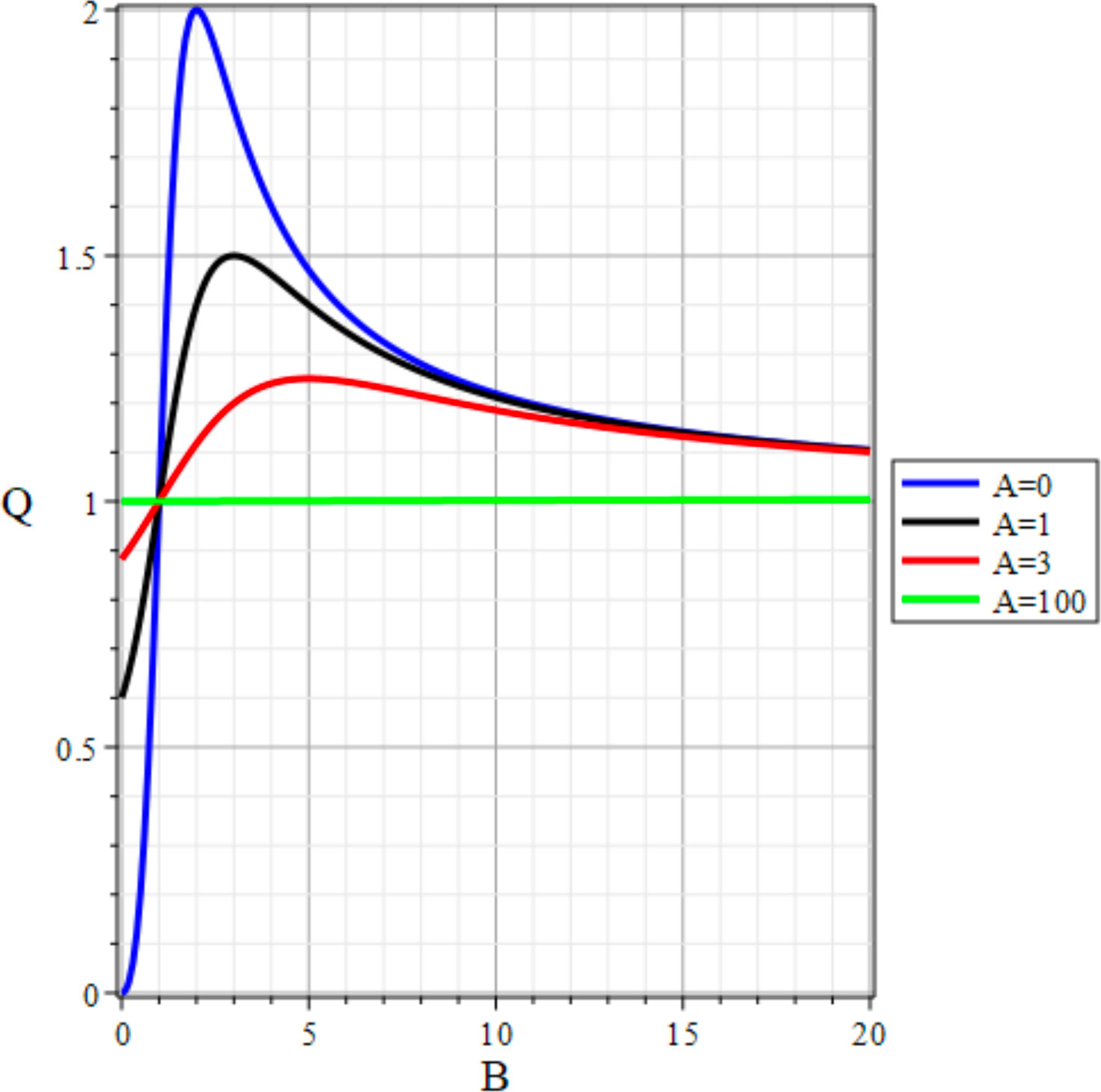
Figure 4 Attenuation rate $Q$ as a function of nondimensional imaginary Robin parameter B for various values of nondimensional real Robin parameter $A$.

One classic (and striking) result in Figure 4 is that the maximum nondimensional attenuation rate becomes twice as large as inextensible limit when $A=0$ (blue line), i.e., when the Robin parameter is purely imaginary and positive. This is related to the excitation of longitudinal elastic, or dilational, waves at the surface (i.e., Equation 9). Dilational waves in thin surface films efficiently dampen short waves—an intriguing phenomenon that has been the subject of study since antiquity (see, e.g., the historical review by Scott, 1977). From Miles (1967), generalizing an earlier result by Dorrestein (1951), we can write in our notation for an insoluble visco-elastic monolayer at the surface:

$\begin{array}{ll}\partial u/\partial z+\partial w/\partial x+[({\zeta }_1+{\zeta }_2)k^2/(\rho \nu )+i{E}_{*}{k}^2/(\nu \omega )]u=0, z=\mathrm{0,}& (30)\end{array}$

where $E_{*}$ is the surface elasticity per unit density, and ${\zeta }_1$and ${\zeta }_2$ are the dilatational and shear viscosities of the film; see also Miles (1991). Comparing with Equation 1, we note that here

$\begin{array}{ll}{R}_r=({\zeta }_1+{\zeta }_2)k^2/(\rho \nu ),& (31)\end{array}$

$\begin{array}{ll}{R}_i=E_{*}{k}^2/(\nu \omega ).& (32)\end{array}$

We thus see that the Robin boundary condition (Equation 1), with $R_r,R_i>0$, is related to the viscoelastic properties of the surface cover in that the real part of the Robin parameter represents the viscous effects (as we already have explored), while the imaginary part captures the elastic properties of the cover. This means that R_i, and hence B, must be positive since a negative value of the elasticity is unphysical. Miles (1991) was the first to point out that the coefficient in Equation 24 was a complex quantity.

In the film problem, we take that the surface viscosities are negligibly small (Dorrestein, 1951; Lucassen, 1968). Hence, the Robin parameter is purely imaginary. From Equation 23 we then have that

$\begin{array}{ll}Q=B^2/(B^2-2B+2).& (33)\end{array}$

The maximum value is $Q=2$ when $B=2$, as seen in Figure 4. Introducing the dimensionless parameter $\delta =\gamma k^2{E}_{*}/{\omega }^2$ (Dorrestein, 1951), we have from Equation 32 that $B\equiv R_i/\gamma =2\delta$. Hence, we obtain from Equation 21 for pure temporal damping, when $2k/\gamma$ is small, that ${\widehat{\beta }}_{max}=Q_{max}=2$ for $\delta =1$, which is Dorrestein’s classic result.

Since the wave modes are coupled, Equation 21 yields the damping rate for both the dilational and surface waves.

Jenkins and Jacobs (1997) compare Equations 30 and 27 and conclude that Equation 30 has exactly the same properties as Equation 27 regarding wave damping if we replace $({\zeta }_1+{\zeta }_2)k^2/(\rho \nu )+i{E}_{*}{k}^2/(\nu \omega )$ in the film case by $4d{k}^2{\mu }_s/\mu$. However, as shown here, this is not true since the elastic film case has a dominant imaginary Robin part yielding increased damping (Figure 4, blue line), whereas in the viscous layer case, the Robin parameter is real.

5 The energetics of dilational wave damping

As mentioned, the increased maximum damping for a certain R_i as seen in Figure 4, is related to the existence of dilational waves (Lucassen, 1968; Weber and Christensen, 2003). Free dilational waves are critically damped through viscous dissipation in the oscillatory boundary layer. For this reason, the linear dispersion relation differs depending on whether the dilational waves are (i) damped in time, (ii) damped in space, or (iii) sustained by an undulating stress at the surface, i.e., forced waves (Weber and Christensen, 2003). Surface waves provide just such a mechanism for sustaining the dilational waves, and the dilational wave frequency relevant here is given by the dispersion relation for forced waves:

$\begin{array}{ll}{\omega }_D=[k{}^4{E}_{*}^2/(2\nu )]{}^1{/}^3.& (34)\end{array}$

In the present problem, where maximum damping occurs for $B=R_i/\gamma =2$, we find from Equation 34), by using Equations 13 and 32, that

$\begin{array}{ll}{\omega }_D=\mathit{\omega .}& (35)\end{array}$

Hence, as pointed out in Christensen (2005), maximum damping occurs when the natural frequency of the forced dilational waves exactly coincides with the natural frequency of the surface waves. Physically, the dilational waves, which would, in the absence of surface waves, be nearly critically damped, act as a sink of energy for short gravity waves. This phenomenon is sometimes referred to as “negative resonance”. Similar behaviors appear in more complex setups, for example, the case of finite layer thickness with two elastic interfaces, for which two damping maxima are possible (Ermakov and Khazanov, 2022).

We can gain more insight into the role of dilational waves as an energy sink if we split the horizontal velocity components into two parts $u=\tilde{u}+\widehat{u}$, representing the surface wave (Equation 8) and the dilational wave (Equation 9), respectively. The presence of the dilational wave makes the amplitude of the total horizontal velocity $u$ dependent on the elasticity parameter. Maximum damping is associated with a maximum in the horizontal velocity $u$, and hence a maximum in the work per unit time done by the surface stress (Equation 25). The dissipation is primarily due to the strongly sheared dilational wave motion:

$\begin{array}{ll}D\approx \widehat{D}= \rho \upsilon \underset{-\infty }{\overset{0}{\int }}\overline{{(\partial \widehat{u}/\partial z)}^2}dz=\rho \upsilon \underset{-\infty }{\overset{0}{\int }}\overline{[\partial /\partial z[\widehat{u}(\partial \widehat{u}/\partial z)]-\widehat{u}({\partial }^2\widehat{u}/\partial z^2)]}dz.& (36)\end{array}$

The surface stress is well approximated by $\tau =\rho \upsilon \partial \widehat{u}/\partial z(z=0)$. We now define the work per unit time on the oscillatory boundary layer:

$\begin{array}{ll}\widehat{W}=\overline{\tau \widehat{u}}=\rho \upsilon \overline{\widehat{u}(\partial \widehat{u}/\partial z)}, z=0.& (37)\end{array}$

The second term on the right-hand side of Equation 36 is zero because of $\widehat{u}$ and ${\partial }^2\widehat{u}/\partial z^2$ always being 90° out of phase, cf. Equations 9 and 13. From Equations 36 and 37, we find that $\widehat{W}=\widehat{D}$ as we would expect for dilational waves (Weber and Christensen, 2003), which means that although the dilational waves are continuously excited by the surface waves, being coupled through the surface condition (Equation 1), they are continuously being dissipated in the oscillatory boundary layer at the same rate.

6 Concluding remarks

To model the various effects that may change the physics of the ocean surface, and hence affect growth and decay of surface waves, we have related the shear stress at the water surface and the horizontal velocity using a Robin condition with a complex Robin parameter. Using known results for viscous fluid layers and elastic monolayers, we show how the real part of the Robin parameter is related to viscous or frictional surface effects, while the imaginary part is associated with surface elasticity. In many situations of practical interest, for instance for ice covered waters, large floating mats of seaweeds, or more complex sea slicks with anisotropic horizontal distributions of surfactant, the dynamical conditions at the surface quickly become very complex, and we need to resort to simplified parameterizations of average behavior, particularly on the horizontal scales of numerical wave prediction models. Since it is practically impossible to formulate a unified mathematical theory explaining the effect of surface constituents on surface waves, or even to formulate constitutive relations, we may resort to modeling the interaction between the surface waves and the floating materials by applying the Robin condition and adapting the Robin parameter to the problem in question. Even if a quantitative estimation of the Robin parameter is not possible, a discussion of the problem for limiting values of $R$ may still improve our understanding of the basic physics involved.

Data availability statement

The original contributions presented in the study are included in the article/supplementary material. Further inquiries can be directed to the corresponding author.

Author contributions

JW contributed the original idea behind this study. JW and KC contributed equally to the mathematical analysis and writing. Both authors contributed to the article and approved the submitted version.

Funding

Financial support from the Research Council of Norway through the grants 280625 (Dynamics of floating ice) and 314449 (ACTION) is gratefully acknowledged.

Conflict of interest

The authors declare that the research was conducted in the absence of any commercial or financial relationships that could be construed as a potential conflict of interest.

Publisher’s note

All claims expressed in this article are solely those of the authors and do not necessarily represent those of their affiliated organizations, or those of the publisher, the editors and the reviewers. Any product that may be evaluated in this article, or claim that may be made by its manufacturer, is not guaranteed or endorsed by the publisher.

References

Akin J. E. (2005). Finite element analysis with error estimators: An introduction to the FEM and adaptive error analysis for engineering students. Elsevier Butterworth-Heinemann. doi: 10.1016/B978-0-7506-6722-7.X5030-9

CrossRef Full Text | Google Scholar

Christensen K. H. (2005). Transient and steady drift currents in waves damped by surfactants. Phys.Fluids 17, 9. doi: 10.1063/1.1872112

CrossRef Full Text | Google Scholar

Dorrestein R. (1951). General linearized theory of the effect of surface films on water ripples. Proc. K. Ned. Akad. Wet. Ser. B: Palaeontol. Geol. Phys. Chem. Anthropol. B 54, 260; 54, 350.

Google Scholar

Ermakov S. A., Khazanov G. E. (2022). Resonance damping of gravity-capillary waves on water covered with a visco-elastic film of finite thickness. a reappraisal. Phys. Fluids 34, 092107. doi: 10.1063/5.0103110

CrossRef Full Text | Google Scholar

Gade M., Hühnerfuss H., Korenowski G. (2006). Marine surface films: Chemical characteristics, influence on air-Sea interactions and remote sensing (New York: Springer, Berlin Heidelberg).

Google Scholar

Gustafson K. (1998). Domain decomposition, operator trigonometry, robin condition. Contemp. Math. 218, 432–437. doi: 10.1090/conm/218/3039

CrossRef Full Text | Google Scholar

Hahn D. W., Ozisk M. N. (2012). Heat conduction. 3rd edition (New York: Wiley).

Google Scholar

Jenkins A. D. (1986). A theory for steady and variable wind- and wave-induced currents. J. Phys. Oceanogr. 16, 1370–1377. doi: 10.1175/1520-0485(1986)016<1370:ATFSAV>2.0.CO;2

CrossRef Full Text | Google Scholar

Jenkins A. D., Jacobs S. J. (1997). “Wave damping by a thin layer of viscous fluid”. Phys. Fluids 9, 1256–1264. doi: 10.1063/1.869240

CrossRef Full Text | Google Scholar

Lamb H. (1932). Hydrodynamics. 6th ed (Cambridge, UK: Cambridge University Press).

Google Scholar

Lucassen J. (1968). Longitudinal capillary waves, part 1-theory. Trans. Faraday Soc 64, 2221–2229. doi: 10.1039/TF9686402221

CrossRef Full Text | Google Scholar

Marsh R., Oxenford H. A., Cox S. A., Johnson D. R., Bellamy J. (2022). Forecasting seasonal sargassum events across the tropical Atlantic: overview and challenges. Front. Mar. Sci. 9. doi: 10.3389/fmars.2022.914501

PubMed Abstract | CrossRef Full Text | Google Scholar

Martin S., Kauffman P. (1981). A field and laboratory study of wave damping by grease ice. J. Glaciol. 27, 283–313. doi: 10.1017/S0022143000015392

CrossRef Full Text | Google Scholar

Miles J. W. (1967). Surface-wave damping in closed basins. Proc. R. Soc A 297, 459–475. doi: 10.1098/rspa.1967.0081

CrossRef Full Text | Google Scholar

Miles J. W. (1991). A note on surface films and surface waves. Wave Motion 13, 303–306. doi: 10.1016/0165-2125(91)90066-W

CrossRef Full Text | Google Scholar

Scott J. C. (1977). The historical development of theories of wave-calming using oil. Hist. Technol. 3, 163–186. doi: 10.5040/9781350017429.0011

CrossRef Full Text | Google Scholar

Squire V. A. (1984). Sea Ice. Sci. Prog. Oxf. 69, 19–43.

Google Scholar

Sutherland G., Rabault J., Christensen and A. Jensen K. H. (2019). A two layer model for wave dissipation in sea ice. Appl. Ocean Res. 88, 111–118. doi: 10.1016/j.apor.2019.03.023

CrossRef Full Text | Google Scholar

Tyvand P., Nøland J. K. (2019). Onset of convection in a triangular porous prism with robin-type thermal wall condition. Transp. Porous Med. 130, 751–767. doi: 10.1007/s11242-019-01337-4

CrossRef Full Text | Google Scholar

Weber J. E. (1983). Steady wind-and wave-induced currents in the open ocean. J. Phys. Oceanogr. 13, 524–530. doi: 10.1175/1520-0485(1983)013<0524:SWAWIC>2.0.CO;2

CrossRef Full Text | Google Scholar

Weber J. E. H. (2022). A note on the temporal and spatial attenuation of ocean waves. Ocean Model. 175, 102027. doi: 10.1016/j.ocemod.2022.102027

CrossRef Full Text | Google Scholar

Weber J. E. H., Børve E. (2021). Diurnal continental shelf waves with a permeable coastal boundary: Application to the shelf northwest of Norway. Eur. J. Mech./B Fluids 86, 64–71. doi: 10.1016/j.euromechflu.2021.05.003

CrossRef Full Text | Google Scholar

Weber J. E., Christensen K. H. (2003). Mean drift induced by free and forced dilational waves. Phys. Fluids 15, 3703–3709. doi: 10.1063/1.1621867

CrossRef Full Text | Google Scholar