Simultaneous tracking of multiple whales using two fiber-optic cables in the Arctic

1 Introduction

Baleen whales play crucial ecosystemic roles in the oceans, from predators to prey, climate regulators, nutrient reservoirs, niche constructors enhancing biodiversity, and connectors between ecosystems (Lavery et al., 2014; Roman et al., 2014). After being brought to the brink of extinction, many species are recovering following the cessation of large-scale commercial whaling (Thomas et al., 2016). Nevertheless, their recovery is hampered by anthropogenic stressors associated with modern and industrialized ocean exploitation where pollution (acoustic, chemical, and thermal) coupled with ocean acidification, add to the primary threats of ship strikes and entanglement in fishing gear (Greene and Pershing, 2004; Thomas et al., 2016).

In the Arctic, the climate is changing faster than anywhere else in the world (IPCC, 2022), and the Svalbard archipelago is one of the fastest warming regions (Maturilli et al., 2013; Nordli et al., 2014). This can be observed in many ways; e.g., through the rapid retreat of glaciers in the Svalbard area (Hagen et al., 1993; Schuler et al., 2020) and by the decrease in Arctic sea-ice (Stroeve et al., 2007; Comiso et al., 2008). The “Atlantification” of the Arctic alters sea-surface temperatures and circulation patterns, forcing some cetaceans to change their seasonal habits; e.g., the timing of their migration, the migration route itself, or even forcing them to seek alternative habitats (van Weelden et al., 2021). This impacts both endemic Arctic species and boreal visitor species (Hamilton et al., 2021); e.g., fin whales have recently been observed to change their observed presence in Arctic regions from late spring/early summer to the fall to year-round (Klinck et al., 2012). At the same time, human activities, their intensity, and impacts are also evolving with sea-ice loss; e.g., with the impending development of cross-Arctic shipping routes and openings for natural resource exploitation (Jaskolski, 2021; Townhill et al., 2022). Hence, we can expect that human activities will intensify in species-rich areas (Hamilton et al., 2021).

Considering the region’s dynamism, it is urgent to develop robust and scalable methods to draw the baseline of species’ geographic range and habitat use to understand their ecology, which is challenging for highly mobile and pelagic baleen whales (Ahonen et al., 2021). The methods should also enable close to real-time monitoring to identify rapid changes and mitigate anthropogenic impacts. A key element is to be able to evaluate whales’ positions both at large- and fine-scales. Current and common methods for tracking baleen whales include visual surveys (Cummings and Thompson, 1971), satellite tracking (Lydersen et al., 2020; Hoschle et al., 2021) or deploying widespread arrays of hydrophones to determine a whale’s position from time difference of arrival and hyperbolic intercepts of its calls (McDonald et al., 1995). Nowacek et al. (2016) presents a review of recent technologies used for conservation-oriented behavioral studies of cetaceans while Harcourt et al. (2019) focuses specifically on methods applied to the conservation of right whales. Under the scope of localization and tracking, passive acoustic monitoring (PAM), using long-term hydrophone installations or towing arrays during short field trial periods, has proven reliable and cost-effective and has been used extensively since the late 1980’s to quantify the seasonal presence of whales (Sirovic et al., 2013; Ahonen et al., 2021) and to estimate locations (see, e.g., McDonald and Fox (1999); Thode et al. (2000); Bouffaut et al. (2021)). However, individual hydrophones are often unevenly spaced, making fine-scale movement analysis difficult, and they are often sparse, resulting in undersampling of the vast ocean habitat of baleen whales (Ahonen et al., 2017; Ahonen et al., 2021). The sparse instrumentation can be largely attributed to the cost of purchasing, installing and maintaining these systems and the finite life span of their batteries. Therefore, we are in need of continuous-monitoring PAM systems that are cost-effective, spread over large areas and with sufficient spatial density to fill the gaps in existing capabilities. In addition, it would be highly desirable to be able to get measurements in near-real-time, rather than having to wait until recording instruments are recovered.

Over the last two decades, a new technology, Distributed Acoustic Sensing (DAS), has emerged as a game-changer in remote acoustic sensing, with the potential to fill many of the monitoring gaps in the ocean. Connecting an ‘interrogator’ to the end of a ‘dark’ (unused) fiber in a fiber-optic cable allows acoustic data to be acquired continuously. Virtual acoustic sensors can be generated at spatial intervals along the cable as frequently as every meter, for up to 171 km along the fiber (Waagaard et al., 2021). Over 1.3 million km of offshore telecommunication cables are installed worldwide, creating an opportunity to increase remote acoustic sensing coverage both onshore and offshore. Currently, these virtual sensors do not have the sensitivity to rival dedicated hydrophones. However, with thousands lying along an extended cable, the beamforming gain available through signal processing, together with the ability to ‘focus’ on sources using the very long array, offers unique potential. DAS technology has already been applied to many different fields ranging from earthquake seismology (Lindsey et al., 2017) to geophysical exploration (Mestayer et al., 2011; Taweesintananon et al., 2021), near-surface monitoring (Dou et al., 2017), oceanography (Taweesintananon et al., 2023), water-born sound sources (Matsumoto et al., 2021), and passive acoustic monitoring of ships (Rivet et al., 2021) and baleen whales (Bouffaut et al., 2022; Landrø et al., 2022). Until recently, DAS has been collected from single fibers. However, there is growing interest in combining two different fibers, either in the same or in separate telecommunication cables, when configuration and access allow it (Wilcock et al., 2023).

Fiber-optic cables are often trenched for protection against anchoring and fish trawling. Depending on the sea bed type, the cables are usually laid in a line that covers the shortest possible distance to minimize cost and reduce latency. When interrogating straight-line cable segments, we generally encounter the well-known left-right ambiguity (also known as 180° ambiguity) associated with linear arrays, in which it is impossible to determine which side of the array the source is located. Bouffaut et al. (2022) experienced this problem when tracking whales using the inner cable between Longyearbyen and Ny-Ålesund from a similar experiment in 2020 and Landrø et al. (2022) had the same issue when tracking a cargo ship. While it may sometimes be possible to resolve the left-right ambiguity if the environment breaks the symmetry, the only sure solution is to make the array two-dimensional. This can be achieved by curving the array (as it negotiates a ‘corner’, for example) or using a second array separated by a sufficient distance to provide a resolvable time of arrival difference, yet close enough to receive the same source signals. We exploit the availability of two such cables in this work.

We investigate and compare two different methods to track baleen whales using DAS: a Grid Search (GS) method (Havskov and Ottemoller, 2010) and a Bayesian Filter (BF; see, e.g., Sarkka (2013)). These two methods were applied to data recorded on two fiber-optic cables connecting Longyearbyen and Ny-Ålesund in the Svalbard archipelago (Figure 1). We first exploited the ground truth generated by a single geo-referenced air gun source for calibration and evaluation of the accuracy of these two methods. A small air gun was used, in accordance with the permissions given by the authorities in Svalbard, to minimize disturbance and potential harm to marine life. Then, over a 5.1 h period recorded on a 60 km portion of the cable, up to eight fin whales (Balaenoptera physalus) were successfully tracked.

FIGURE 1

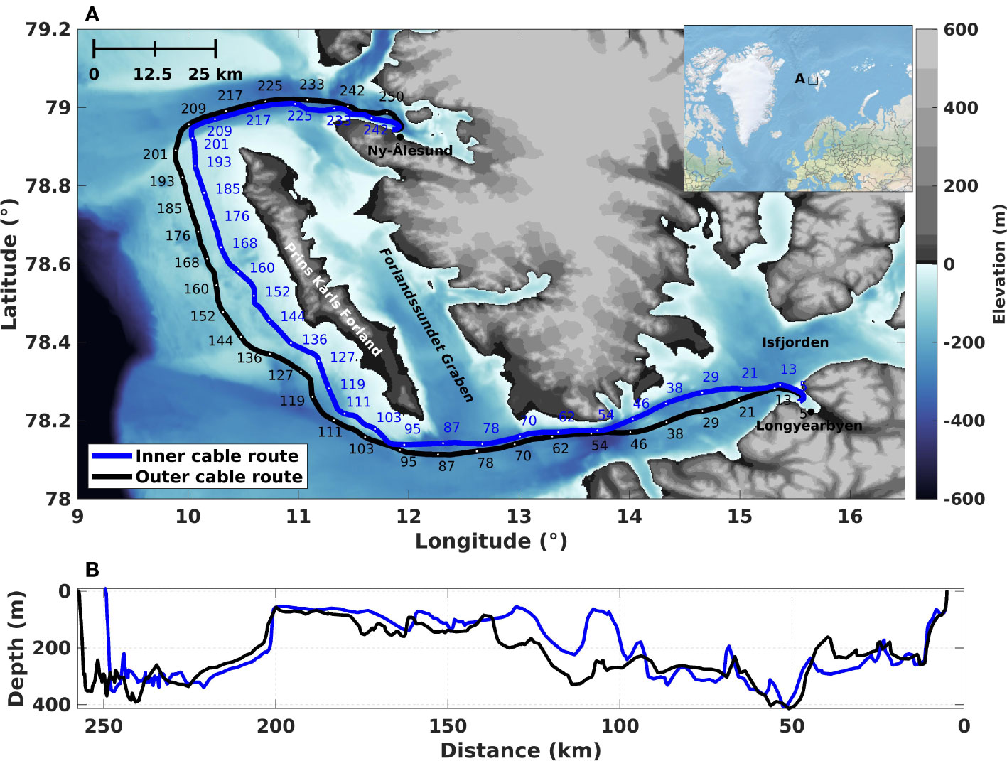
Figure 1 An overview map of the study area. (A) The fiber-optic telecommunication cables are located between Longyearbyen and Ny-Ålesund. Starting in Longyearbyen, the cables enter the Adventsfjorden 5 km after the interrogator unit; they then cross Isfjorden into the open ocean, bypassing Prins Karls Forland before entering the Kongsfjorden north of the settlement at Ny-Ålesund. The entire length of both telecommunication cables was interrogated using four interrogator units. However, only data from the two units located in Longyearbyen have been used in this work. (B) The ocean depth profiles along the fiber paths, the cables are trenched an additional 0-2 m into the seafloor.

The paper is organized into five main parts. First, the distributed acoustic sensing data is presented, where the experimental set-up, the air gun, and fin whale data are introduced. The second part contains information on the methods used to obtain the results. The data conditioning, time of arrival picking and computation of empirical detection range are first presented, followed by the localization methods, the GS and the BF. Then, the results from the air gun and fin whale tracking are given, as well as individual fin whale song characteristics. The results are discussed in part four. Firstly, the localization errors are discussed, followed by comparing the two localization methods and DAS-based localization for whale conservation. Finally, we present some conclusions.

2 Distributed acoustic sensing data

2.1 Experimental set up

Currently, it is common practice to include more optical fibers than initially required within one fiber optic telecommunication cable, to enable network growth and increase redundancy at a minimal incremental cost. Using Alcatel Submarine Network OptoDAS interrogators, we tapped into two out of 24 standard single mode G.652D fiber bundles within each of two existing submarine telecommunication cables connecting Longyearbyen and Ny-Ålesund in Svalbard, Norway (Figure 1). The OptoDAS interrogators send linear optical frequency-modulated swept pulses into the fiber and interrogate the Rayleigh backscattering caused by inherent inhomogeneities in the fibers (Waagaard et al., 2021). Such inhomogeneities are displaced by, e.g., acoustic waves from whales impinging on the fiber, which can be detected as phase changes in the Rayleigh backscatter. The time-differentiated phase is obtained by continuously comparing the backscattered response from one pulse to the next. This is typically done in two steps: first, the phase is spatially differentiated between regularly spaced channels along the optical fiber, then compared to the next pulse’s response. The time-differentiated phase is stored by the interrogator and later converted to fiber strain during the data processing (see, e.g., Hartog (2017), for more information on this conversion). Normal signal strength decay along the fiber is about 0.2 dB/km, depending on the quality of the optical fibers and connectors. The returned signal strength from 100 km is, therefore, ≃-40 dB with respect to 1 km. To date, the maximum cable length that has been interrogated with a signal above the noise floor is 171 km, applying low-loss cables. On commercial telecommunication cables, the range is typically 140–150 km (Waagaard et al., 2021). Therefore, to collect data on the entire 260 km length of each separate telecommunication cable, four interrogator units were deployed; two in Ny-Ålesund and two in Longyearbyen, one for each direction on each telecommunication cable. Both optical fibers were dark, i.e., not used for data transfer. We denote the two telecommunication cables as the ‘inner cable’ (the cable closest to Prins Karls Forland) and the ‘outer cable’ (the cable furthest from Prins Karls Forland; see Figure 1). The first 5 km portions of the telecommunication cables at the Longyearbyen and Ny-Ålesund ends are trenched on land. The subsequent 248 km portion of the inner cable and the 252 km for the outer cable are sub-sea cables buried 0–2 m below the seafloor. Only data recorded on the sub-sea part of the telecommunication cables have been analyzed in this work.

The four interrogators were installed over two periods in the summer of 2022. The first interrogator started recording in Ny-Ålesund 2022.06.02 and is still recording as of 2023.03.20. The latter three were installed roughly two months later, the first two in Longyearbyen on 2022.08.17 and the last unit on 2022.08.19 in Ny-Ålesund. The OptoDAS interrogators were each connected to a different optical fiber within the inner and outer telecommunication cables. The same optical fiber was not used with more than one interrogator for two reasons: (1) The laser pulses emitted by an interrogator at one end of a fiber could damage a unit connected to the same fiber at the other end. (2) There could be unknown interference effects arising from two overlapping laser pulses traveling in opposite directions in the same fiber. All four interrogators used a gauge length of 8.16 m with virtual channels sampled every 4.08 m over a 136 km distance. The recorded data were transferred near-real-time to NTNU in Trondheim, Norway, using the network infrastructure described in Landrø et al. (2022). The data were also saved locally on Network Attached Storage (NAS) discs on the interrogator units as a backup. We used light pulses with a free-space wavelength of 1550 nm with a sampling period of 1×10⁻⁸ s at the optical receiver. The data were recorded at a sampling frequency of 625 Hz. The interrogated distance ensured that the entire length of both telecommunication cables was covered, with a ≃10 km overlap east of Prins Karls Forland (roughly ±5 km of the 130 km mark in Figure 1A). The three interrogators installed in mid-August recorded data continuously for roughly two months (with some breaks due to, e.g., power outages) before being shipped back to mainland Norway. Only data recorded by the interrogators in Longyearbyen have been analyzed in this work.

2.2 Air gun data

A dedicated air gun survey was performed on 2022.09.06 to allow us to estimate the errors related to the two localization methods used in this work. Permission was given by the authorities in Svalbard to minimizing disturbance and potential harm to marine life. No whale vocalizations were observed in the DAS data from the survey period. The air gun was towed 10 m behind the ship, which recorded its position every second from an onboard Global Positioning System (GPS).

The chamber of the air gun was 0.1311 m³ (20 in³), and the average chamber pressure used was 12000 kPa (120 bar), producing a source of 100–200 kPa-m (1–2 bar-m; the pressure one meter from the source, corresponding to 220 dB re. 1 μPa at 1 m). Note that fin whale source levels observed along the Norwegian coast is reported to be $190.5\pm 7.4$ dB (Garcia et al., 2019). The air gun shots produced a valuable data set that we have used to calibrate the analysis in this paper.

The air gun data were acquired for roughly 3.5 h on 2022.09.06 with an inter-shot interval of ≃60 s (with some longer breaks due to malfunctions in the acquisition system), resulting in a total of 183 shots. For this work, we selected a 41-shot sub-set covering source locations above each cable and in between (see Figure 2). When fired directly above one of the cables, an air gun signal could be observed over ≃6 km in each direction along the cable as well as on the adjacent fiber optic cable if the inter-cable distance was lower than 6 km (see Supplement Material Figure S1A for an example of a recorded air gun shot). It is possible to increase the detection range by applying a filter in the frequency-wavenumber domain (f-k filter), which provides processing gain.

FIGURE 2

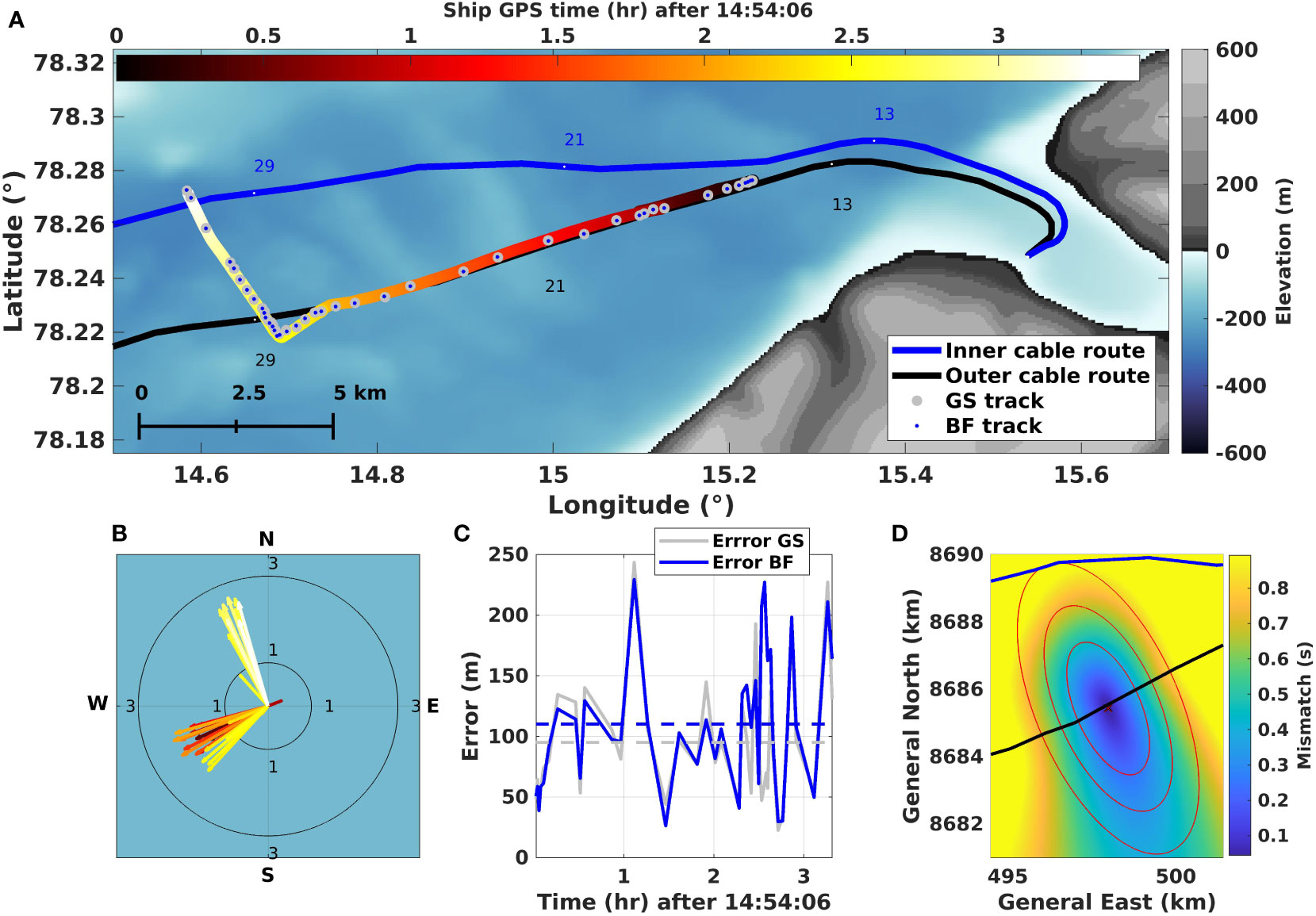
Figure 2 Tracking the air gun with known shot locations. (A) Overview of the first 35 km section of cables, showing ship track, color-coded from dark to light (by origin time of shots) overlaid with the estimates from the grid search (GS; big gray circles) and the Bayesian filter (BF; small blue circles). (B) The associated velocities of the ship are estimated by the BF with the same color coding as (A). (C) The error between the estimated location and the known position of the ship at the shot origin time. (D) RMS mismatch from GS overlaid by the error ellipse (1x, 2x, 3x standard deviation) from the BF based on a representative shot with an error (100 m) close to the mean error of all shots.

2.3 Fin whale data

To test our methods for baleen whale tracking, we selected a 5.1 h portion of the DAS dataset acquired on 2022.08.22 that proved to contain 1808 fin whale 20 Hz-calls. Note that we performed laser sweep calibrations on both interrogator units between 11:13 and 11:23 on that day. The fin whale song is described in the literature as a series of 20-Hz-centered down sweeps of ≃ 1 s duration (Thompson et al., 1992; McDonald et al., 1995). These calls, thought to be produced only by males, have been recorded around Svalbard between July and September/October (Ahonen et al., 2021), in association with local ship-based visual surveys. A subset of 188 calls was used to demonstrate the feasibility of using two parallel fiber-optic cables to track several whales simultaneously.

Figure 3 shows an example of a fin whale 20 Hz-call series recorded over a 90 s time window on both the inner and outer cables between 50 and 100 km on 2022.08.22 at 12:27:57 UTC, where (A, B) are spatio-temporal representations underlining the presence of at least three vocalizing whales at ≃60 km, ≃80 km and ≃95 km, (C, D) the waveforms of the calls emitted by the whale at 60 km and (E, F) the associated spectrograms. Note that the distances given (in this case, 50 to 100 km) are the length of fiber from the interrogator to the channel recording the vocalization.

FIGURE 3

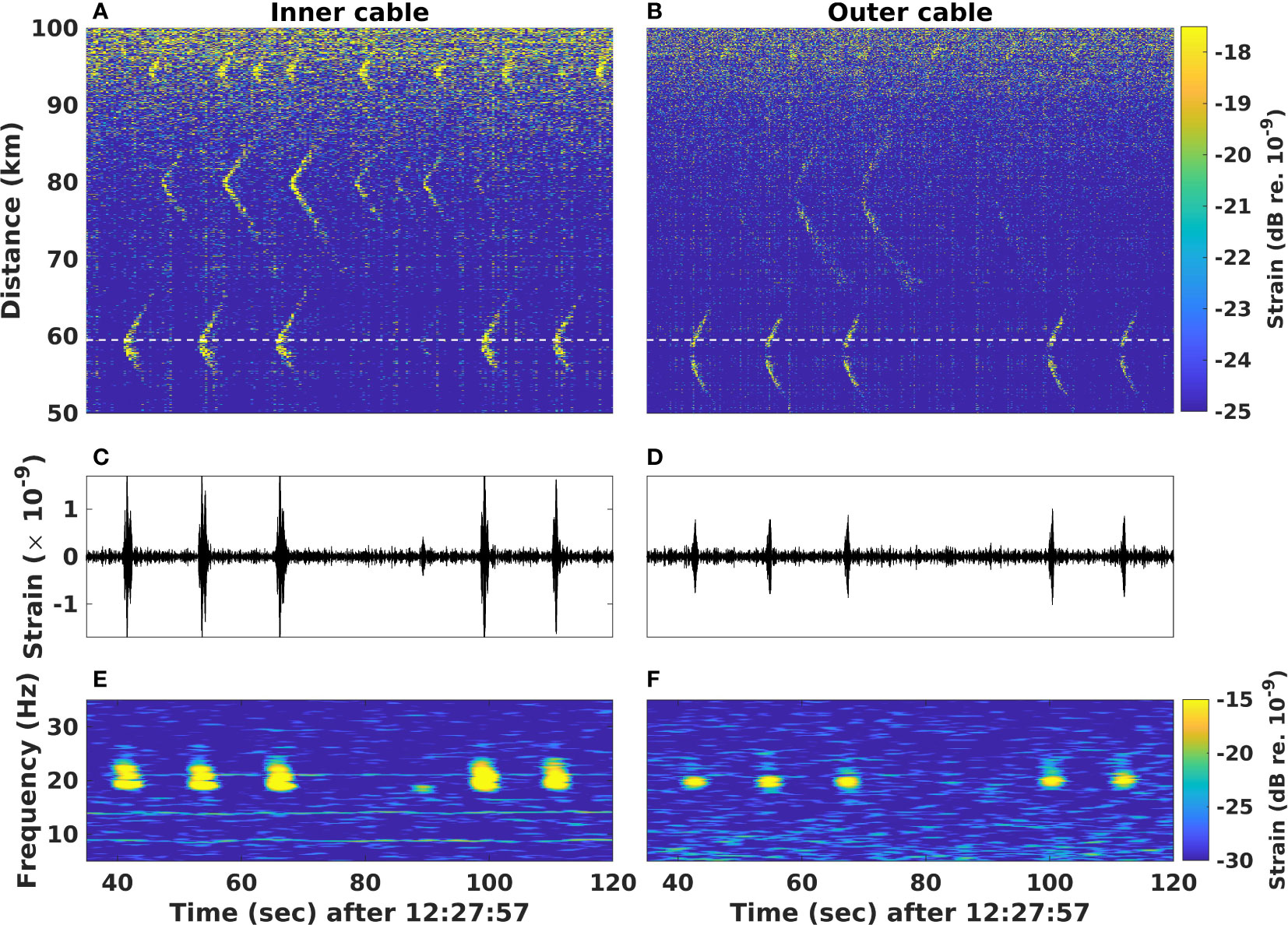
Figure 3 Distributed acoustic sensing recording of fin whale vocalizations on two fiber-optic cables on 2022.08.22 at 12:27:57 UTC. (A, B) Spatio-temporal ($t-x$) representation of three simultaneously vocalizing whales on the inner cable (A) and the outer cable (B) between 50 and 100 km. Waveforms (C, D) and corresponding spectrograms ($t-f$; E, F) at 59.52 km, represented by the white dashed line in (A, B), displaying portions of two series of fin whale 20 Hz calls and a back-beat at ≃95 is recorded on both cables with an average inter-call interval of 13 s. The spectrograms were computed using a Hann window of 512 samples with 98% overlap.

From the repetitive 20 Hz down-sweep signals, their frequency span (between [18-25] Hz) with a duration less than 2 s and average inter-call intervals of 13 s (for the whale at 60 km; the whales at 80 km and 95 km have respective average intervals of 10 s and 9 s), we can clearly identify these as characteristic fin whale 20 Hz song, as well as an example of a back-beat at roughly 90 s (Watkins et al., 1987; Thompson et al., 1992).

3 Methods

3.1 Data conditioning

The following pre-processing steps were carried out to prepare the data for analysis and improve the signal-to-noise ratio (SNR). Initially, the time-differentiated phase was converted to longitudinal strain (Hartog, 2017). Then the data were resampled in time and space to cover the regions of interest. Recorded air gun signals contained frequencies between 5 and 45 Hz, and the sample rate was reduced by a factor of 5, from 625 Hz to 125 Hz. Similarly, the fin whale vocalization carried frequencies between 18 and 25 Hz and was resampled by a factor of 8 to 78 Hz. The data were tapered and band-pass filtered to focus on the frequency band of interest. A Tukey window was applied to the data and subsequently bandpass-filtered using a fourth-order Butterworth filter to focus on each signal of interests’ dominant frequencies. The cut-off frequencies were chosen to focus on the frequency range listed above. Next, a 2D median filter over 3×3 data-points was applied to suppress common-mode noise. Finally, a frequency-wavenumber (f-k) fan filter was applied to preserve only acoustic waves propagating around sound speed in sea-water and sediments, keeping everything with a propagation speed between 1000 and 3000 m/s.

3.2 Time of arrival picking

The data were visually inspected using spatio-temporal representations to identify signals of interest (Bouffaut et al., 2022). This visualization gave an overview of the recorded signals over several channels and was used by one observer to pick the first times of arrivals manually. The first time of arrivals were chosen at a sudden amplitude and frequency changes in the onset of the acoustic signal. To constrain the time of arrival picking burden, a maximum of 12 arrival times were selected from both cables, with an average inter-channel distance between the picks of 600 m (depending on the range from source to receiver). An exact inter-channel distance was not used due to the variation of SNR along the cable. We avoided using arrivals on the tail and focused on arrivals near the apex to avoid picking in the portions of the data dominated by normal modes. However, due to the known directivity of DAS arrays (see, e.g., Papp et al. (2017)), we did not pick arrivals in close vicinity to the apex. When the signal quality from the two cables was significantly different, which was often the case when a whale was vocalizing near one cable, and at a greater distance to the other, fewer picks were selected from the cable with the poorer quality. In the worst cases, we used only one pick from the cable with lower signal strength only to resolve the left-right ambiguity.

3.3 Track estimation

Two different localization methods were developed to estimate the source positions from travel time information detected at the fiber-optic cables: a Grid Search (GS) method and a Bayesian Filter (BF). We denote the observed time of arrivals at the fiber channel locations by $T_{i,j}^{(obs)}$, $i=1,\dots ,n_j$, $j=1,2$. Here, index i refers to the channel used to pick the time of arrival, and j denotes the telecommunication cable used (e.g., $j=1$ corresponds to the inner cable and $j=2$ to the outer cable). Alternatively, one could list these arrival times data in a length $n_1+n_2$ vector, but the i and j index clarify that data are acquired and processed on two different cables.

In the forward model, we assume that a signal is emitted at time $\eta$ from location $(x,y,z)$, where x and y are the geographical coordinates and z is the depth. We use a reference depth of $z=z_{ref}$ set to 20 m for whales (known to be a typical call depth for fin whales (Stimpert et al, 2015) and 3.5 m for the air gun (set prior to the acquisition). The theoretically modelled arrival time, $T_{i,j}(x,y)$, is computed from the origin time of the event studied, $\eta$, and the travel time for the Euclidean distance from the event to the receiver, $t_{i,j}(x,y)$:

$\begin{array}{ll}{T}_{i,j}(x,y)=\eta +t_{i,j}(x,y),& (1)\end{array}$

$$t_{i,j}(x,y)=\frac{\sqrt{{(x-x_{i,j})}^2+{(y-y_{i,j})}^2+{(z_{ref}-z_{i,j})}^2}}{c}.$$

where $(x_{i,j},y_{i,j},z_{i,j})$ is the coordinate of channel i at fiber j and $c=1440$ m/s is the speed of sound in water. The sound speed is based on previous study of Arctic water (Gavrilov and Mikhalevsky, 2006) and the minimum error obtained in the air gun study.

3.4 Grid search position estimation

The GS method uses equally spaced grid points around a prior guess of the source location. Such a systematic search computes the travel time for all possible locations in a survey area to find the best matching source location. This kind of GS procedure has been adapted from earthquake seismology (see, e.g., Havskov and Ottemoller (2010)) and it has been previously applied to earthquakes recorded on DAS arrays by Rørstadbotnen et al. (2022). GS methods are also commonly used for whale localization (see, e.g., Wilcock (2012); Abadi et al. (2017)).

In this work, the grid points are defined from the channels receiving the first signal and laid out on a horizontal grid of (x, y) coordinates. The grid points were set at 25 m intervals, covering a 20 km by 20 km area centered around the receiving channel. For each element of the grid, the reference time $\eta$ is calculated by shifting the computed origin time to the ‘correct’ timing, given by:

$\begin{array}{ll}\eta =\frac{1}{n_1+n_2}\sum _{j=1}^2\sum _{i=1}^{n_j}[T_{i,j}^{(obs)}-t_{i,j}(x,y)].& (2)\end{array}$

When the theoretical travel time and reference time in equation (2) are known for each grid point, the root mean square (RMS) misfit between observed and computed travel times is given by:

$\begin{array}{ll}M(x,y)={(\frac{O(x,y)}{N})}^{1/2},O(x,y)=\sum _{j=1}^2\sum _{i=1}^{n_j}{(T_{i,j}^{(obs)}-T_{i,j}(x,y))}^2,& (3)\end{array}$

where the normalization in the RMS computation is typically performed based on the total number of time of arrival picks used, $N=n_1+n_2$. The estimated location of the source is the grid point with the lowest misfit, i.e., the global minimum RMS across the GS volume. The misfit function depends on the geometry of the source, the time of arrival picks, and cable pick locations.

Rather than evaluating the mismatch on a dense grid, Newton’s method can be used to solve for the position (x, y). Using boldface for vectors and matrices, we start with an initial guess for the position ${\mathit{p}}^0=(x^0,y^0)$ and iterate by:

$\begin{array}{ll}{\mathit{p}}^r={\mathit{p}}^{r-1}-{[\frac{d^{2}l({\mathit{p}}^{r-1})}{d{\mathit{p}}^2}]}^{-1}\frac{dl({\mathit{p}}^{r-1})}{d\mathit{p}},r=1,\dots .& (4)\end{array}$

Here, $l(x,y)=-O(x,y)/2{\tau }^2$ is a statistical likelihood version of equation (3), where we assume that the travel time observations are made with additive independent and Gaussian distributed noise with variance ${\tau }^2$. The guided search provided by equation (4) converges within a few iterations r. We denote the resulting optimum value by $\widehat{\mathit{p}}$. This kind of optimization involves re-setting the reference time $\eta$ (see equation (2)) at each step of the iterative scheme. By investigating residuals from modeled and known air gun shot positions, the noise standard deviation was found to be $\tau =$ 5.4 ms.

A probabilistic view enables uncertainty quantification. In particular, the curvature of $l(\mathit{p})$ at the optimum value can be used to assess the covariance matrix of the position. Together with the optimum, this leads to a Gaussian approximation for the position:

$\begin{array}{ll}\mathit{p}\sim N(\widehat{\mathit{p}},\widehat{\text{Σ}}),\widehat{\mathbf{\text{Σ}}}=-{[\frac{d^{2}l(\widehat{\mathit{p}})}{d{p}^2}]}^{-1},& (5)\end{array}$

where $N\left(\widehat{\mathit{p}},\widehat{\mathbf{\text{Σ}}}\right)$ denotes a normal distribution with mean $\widehat{\mathit{p}}$ and $\widehat{\mathbf{\text{Σ}}}$ covariance matrix holding the variance and covariance of the position estimate. The ellipse-shaped contours of the Gaussian probability density function (PDF) provide a comparison with that achieved using the GS, as shown in Figure 2D. If there is prior information about the position p, a Bayesian approach with a Gaussian approximation for the posterior PDF works similarly.

3.5 State space model and Bayesian filtering

With the association of a state space model and a BF, we can connect the predictions at different locations and also consistently estimate the source speed and direction. Similar uncertainty assessments to travel time data have been applied to, e.g., satellite positioning accuracy (Yigit et al., 2014) and location estimation with borehole seismic data (Eidsvik and Hokstad, 2006).

Let $s_k$, $k=1,\dots$ denote time steps, and represent positions and swim velocities at time $s_k$ by ${\mathit{m}}_k=(x_k,y_k,u_k,v_k)$. Position ${\mathit{p}}_k=(x_k,y_k)$ and east and north velocities $u_k$ and $v_k$ are next coupled over time in a state space model. Travel time data $T_{i,j,k}^{(obs)}$ at time s_k are modelled via the likelihood model $l({\mathit{m}}_k)$ as described below equation (4). Note that measurements carry direct information only about the position ${\mathit{p}}_k$. However, now that a model connects positions and velocities over time, data are implicitly informative about all process variables.

For the dynamical model part, taking state variables from one time to the next, we assume constant velocity and additive noise ${\mathit{\epsilon }}_k$ such that:

$\begin{array}{ll}{\mathit{m}}_k={\mathit{A}}_{k-1,k}{\mathit{m}}_{k-1}+{\mathit{\epsilon }}_k,{\mathit{\epsilon }}_k\sim N(\mathit{0},{\mathit{S}}_{k-1,k}),{\mathit{A}}_{k-1,k}=[\begin{array}{cccc}1& 0& {\text{Δ}}_{k-1,k}& 0\\ 0& 1& 0& {\text{Δ}}_{k-1,k}\\ 0& 0& 1& 0\\ 0& 0& 0& 1\end{array}],& (6)\end{array}$

where the time interval ${\text{Δ}}_{k-1,k}=s_k-s_{k-1}$ and the matrix ${\mathit{S}}_{k-1,k}$ is a $4\times 4$ positive definite covariance matrix for the noise in this process model, accounting for potential acceleration. Equation (6) defines a Markovian structure where the state at time s_k depends on the previous states only through the one at time $s_{k-1}$. An associated formulation of this model in equation (6) is provided by a conditional PDF $p({\mathit{m}}_k|{\mathit{m}}_{k-1})$. Initially, at the time of the first detection, we assume a vaguely informative prior model ${\mathit{m}}_1\sim N(\mathit{\mu },\mathit{\text{Σ}})$, where the mean $\mathit{\mu }$ is composed of the average positions of the cable locations where the first picks are detected and with $0$velocity. The covariance matrix $\mathit{\text{Σ}}$ is set to have significant standard deviations ($1000$ m for positions and $5$ m/s for velocities).

We denote all data available up to time s_k by:

$${\mathit{D}}_k=\left\{T_{i,j,k^{\prime }}^{(obs)};i=1,\dots ,n_{j,k^{\prime }};j=1,2;k^{\prime }\le k\right\}.$$

The data are assumed to be conditionally independent over time. With the Markovian assumptions and that of conditionally independent measurements, methods from Bayesian filtering allow us to estimate the location and velocity ${\mathit{m}}_k$ at a time s_k, given all data up to that time k (see, e.g., Sarkka (2013)). For efficient calculations that can be run online, we fit a Gaussian PDF to the filtering distribution at each observation time. This represents extensions of equations (4) and (5), where the mean of the predictive distribution given earlier data is used to initiate the Newton search. In terms of probability distributions, this means we are approximating the filtering PDF $p({\mathit{m}}_k|{\mathit{D}}_k)$ by a Gaussian model. This filtering procedure is run recursively over time steps $k=1,2,\dots$, and it offers a highly applicable tool for conducting real-time analysis of the travel time data.

By having positions and velocities in a state space model, we can obtain probabilistic state estimates and associated uncertainties at any time s_k, not only at the measurement sites and times.

3.6 Computation of empirical DAS detection range

Using the estimated whale position $(x_w,y_w,z_{ref}=20\text{ m})$ from either the GS or the BF, we estimated an empirical detection range from this position to the position of the DAS channel that detected the last whale signal $(x_{i,j},y_{i,j},z_{i,j})$ before it is lost in the background noise level:

$\begin{array}{ll}{r}_{max}=\sqrt{{(x_w-x_{i,j})}^2+{(y_w-y_{i,j})}^2+{(z_{ref}-z_{i,j})}^2}& (7)\end{array}$

where $r_{max}$ denotes the maximum empirical Detection Range and is taken as a straight line distance.

4 Results

4.1 Air gun tracking

The geo-referenced air gun survey detailed in Section 2.2 is used to calibrate and evaluate the error of both localization methods (Wuestefeld et al., 2018). Figure 2A shows the track obtained from the ship’s GPS overlaid with the locations of the 41 shots as obtained using the grid search (GS; Section 3.4) and the Bayesian filter (BF; Section 3.5). Figure 2B displays the BF estimate of the direction and speed of the ship for the whole track. The warm color scale indicates time on the GPS trajectory on both sub-figures. Figure 2C displays the localization error of each method evaluated for air gun locations 10 m behind the ship’s GPS positions. Figure 2D shows the mismatch between observed and calculated arrival times from the GS overlaid with error ellipses from the BF.

Both methods follow the ship’s track for the selected 3.5 h of recordings. The estimated speed is roughly 1.8 m/s, which agrees with the average speed obtained from the GPS position, 1.9 m/s (see Supplementary Material Figure S1C). There are three areas where the BF underestimates the ship speeds, each associated with the ship making a sharp turn or a loop. In these cases, the BF predictably estimates the ship to travel a shorter distance than it actually does. The estimated mean error standard deviation is $94.9\pm 51.1$ m and $108.8\pm 53.7$ m for the GS and the BF, respectively. Errors are highest when the ship makes turns and when the signal quality on one cable is poor.

4.2 Fin whale tracking

Figure 4A shows the application of the BF to evaluate a fin whale track over an interrupted series of calls (data at 12:07 to 12:14, later referred to as an 8 min portion of whale track B) and Figure 4B the corresponding RMS levels of the calls. The RMS levels are computed in the spatio-temporal domain by a rectangular window enclosing the recorded whale call. For example, for the whale call at 60 km in Figures 3A, B, a rectangular window covering 5 km on each side of the apex and from the start of the apex to 6 s after the apex is used.

FIGURE 4

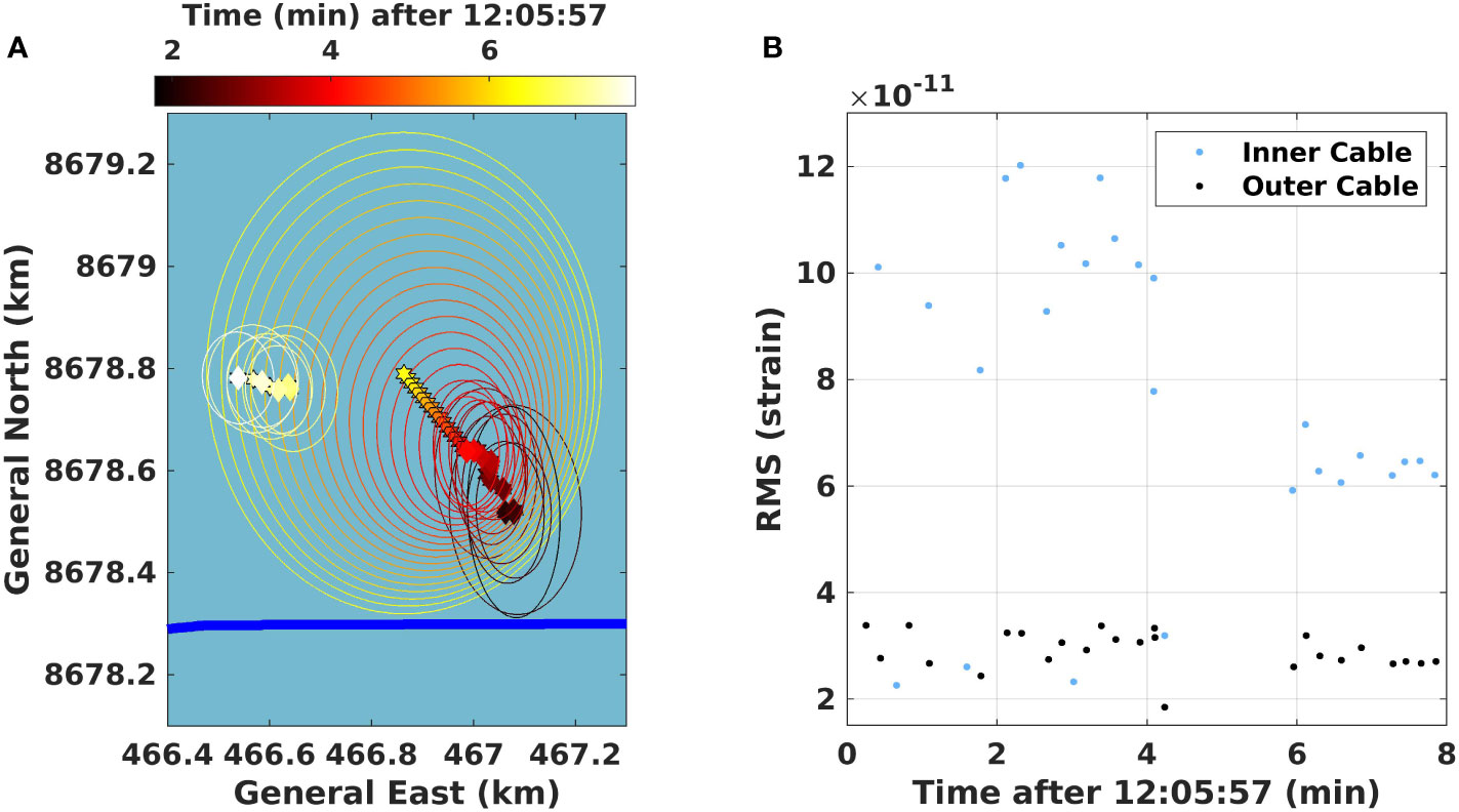
Figure 4 Prediction of whale location during an inter-series interval. (A) A subsection of a whale track near the inner cable (bold blue line; 12:06 – 12:14) with a 1 min 51 s inter-series interval. BF tracks are computed roughly every 10 s, and in inter-pulse intervals, we predict the position without updating (indicated by hexagram). Diamonds indicate the predictions with observed data, while the ellipses show 90% coverage regions constructed by the BF. (B) The associated RMS amplitude of the calls used in the localization.

Each diamond in Figure 4A indicates predictions based on observed data, while hexagrams represent intermediate predictions without observed data. The ellipses correspond to the error expressed in the BF version of equation (5), with a 90% coverage region. The plot shows a portion of whale B’s track lasting roughly 8 min and an Inter-Series interval (ISI) of 117 s. From the BF error ellipses, it is clear that the computed variances decrease as the whale track builds up over many time steps. Locations are computed roughly every 10 s for the track. When the Inter-Call interval (ICI) is longer than 10 s, the BF predicts the location based on the previous track locations and velocities without updated uncertainty. Here, we have an ISI of 2 min, and we compute 12 predictions with a straight-line prediction and increasing uncertainty. When the whale vocalizes after the 2 min pause, the BF finds this new position based on the last prediction, and the new location is within the uncertainty of the prediction. This means that we are, most likely, still tracking the same whale. However, the whale did change course, heading more West during the ISI and it increased its swim speed somewhat, traveling slightly further than the BF prediction. We are thus able to show that interruptions in vocalization can be associated with changes in swim speed and direction.

Figure 5A shows the overview plot of all whale tracks color-coded by the time of vocalizations, where Figures 5B, D, F, H are zoomed-in representations of the tracks, and Figures 5C, E, G, I, the directional swim speeds estimated by the BF. Following the protocol described in the previous paragraph, we found eight distinct whale tracks within the five analyzed hours, denoted by the sequential letters (A) to (F) according to the time of the first vocalization in each track.

FIGURE 5

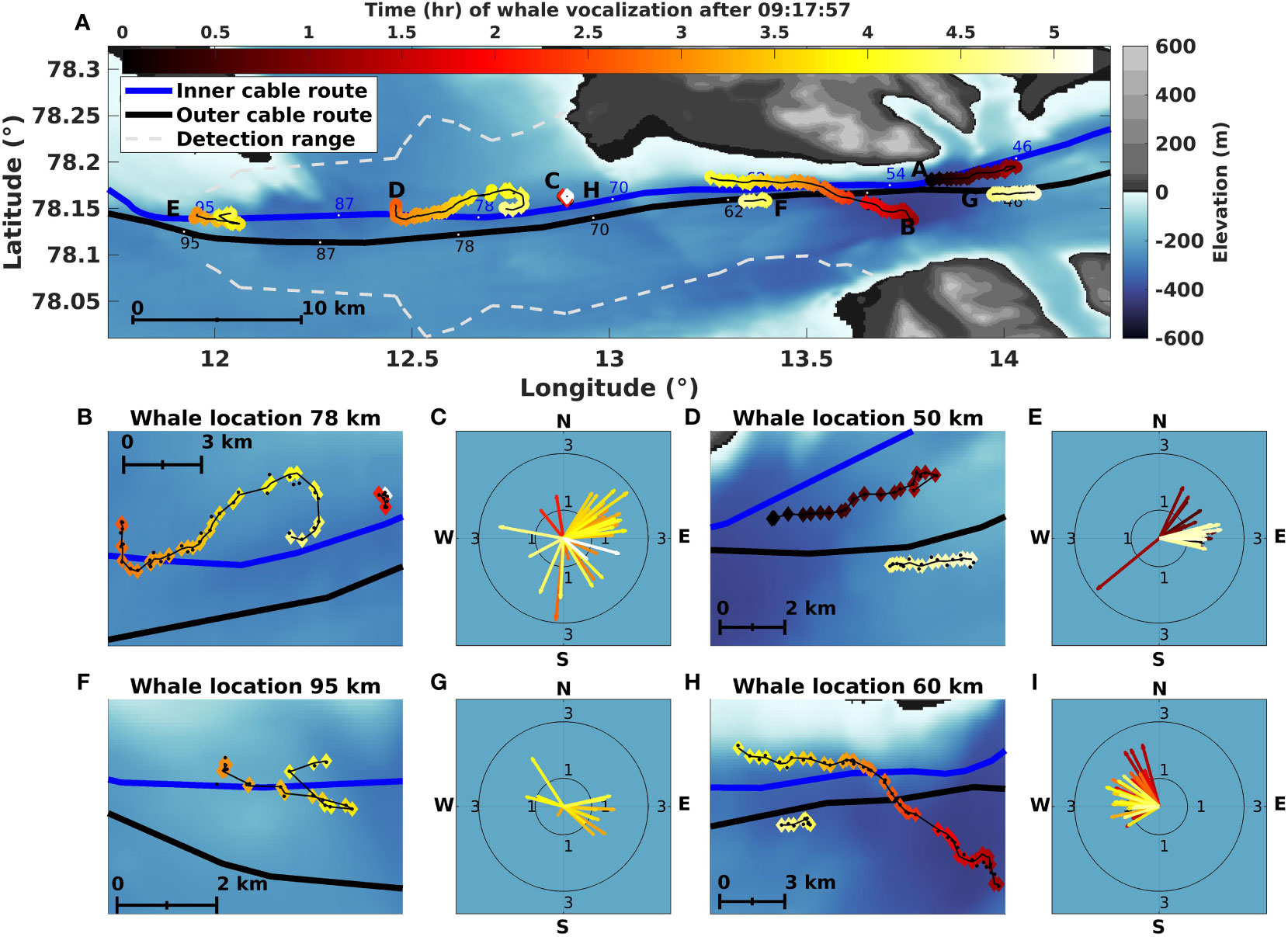
Figure 5 Simultaneously tracking multiple whales using fiber-optic cables in the Arctic. (A) Overview of a 60 km long section of the cables, showing the positions and tracks of up to eight acoustically-detected whales, color-coded from dark to light over a 5.1-hour period. Note that the GS and the BF have been plotted in the same color and shape to better illustrate the tracks. The two dashed lines show an attempt to estimate an empirical whale detection range directly from the DAS data using vocalizations every 10 min for each whale track. (B, D, F, H) Show zoomed-in detailed positions and tracks of the four areas with whale detections. We use the same color coding as in (A) for the BF, while GS has been plotted as black dots to better see the differences in the estimated positions. (C, E, G, I) show the corresponding swim velocities as polar plots for these tracks.

Whale track (A) started at a distance of 50 km from the interrogator unit at 09:28 (all times are given in UTC) and headed East for 72 min before contact loss. Just before losing contact with whale (A), whale track (B) started at 54 km, heading North-West for 160 min before the signal ceased. During this period, we also show the start of a vocalization series from three other positions along the cable, around 60 km, 80 km, and 95 km (see Figure 3), associated with tracks (F), (D), and (E), respectively.

Whale track (C) started around 72 km and headed North. The contact lasted roughly 10 min from 11:23. The interrogator calibration mentioned in Section 2.3 happened between 11:13 and 11:23, and vocalizations from both whale (B) and (C) were lost. No calls associated with whale track (C) are observed in the data prior to 11:13.

Whale track (D) started just after whale track (C), at 11:42, at roughly 80 km from the interrogator unit, lasting 113 min. This track went South before heading North-East over roughly 7 km before looping back West before contact loss. A few vocalizations are localized near track (C) but three hours later (14:20). They are denoted by track (H).

Whale track (E) started the furthest from the interrogator. Calls started at 12:20, South of Prins Karls Forland at 95 km and were detected for 71 min. The background noise level is significant at these long distances, making arrival time picking challenging, especially for the outer cable due to elevated noise and the high inter-cable distance. This increased the uncertainty of the estimated track. Nevertheless, the track headed East for roughly 2.7 km, where it turned and shifted to the North-East. Considering the uncertainty mentioned above and localization error of ≃100 m, two whales could have vocalized simultaneously and parted ways after 1.5 km, one continuing East and the other North-East.

Whale track (F) started at 62 km at 13:30, 18 min after the end of track (B), and headed West. The 4.8 km distance between the two tracks would have required the whale of track (B) to have more than doubled its maximum swim speed (from 2 m/s to 4.4 m/s). While this is not entirely unrealistic (fin whales have been reported to be able to increase swim speed between singing bouts (Clark et al., 2019)) we chose the conservative approach of considering the two tracks separately.

The first column of Figure 6 shows the RMS of received fin whale vocalization amplitudes for whales tracks (B), (C), (D), (F), and (H) over the 5.1 h studied (see Supplementary Material Figure S2 for whales (A), (E), and (G)), calculated as in Figure 4B. We assume that a given fin whale produces 20 Hz songs with an almost stable source level over a short period (Watkins et al., 1987; Garcia et al., 2019). The peaks traced out by the RMS values of detected strain reflect the fact that whale B crosses the outer fiber at a more perpendicular angle than the inner cable, the second peak being less sharp than the first. The minimum strain at which we can detect the vocalizations is observed to be $\simeq 2\times {10}^{-11}$, which constrains the maximum detection range. It is also interesting to note that the RMS amplitude peak of the two whale B crossings are similar, indicating that the two cables have similar sensitivities. The second column in Figure 6 shows a zoomed-in version of the calls of whale tracks (B) and (D) to illustrate the ICI and the ISI (for the same plot for whales (A) and (E) see Figure S2).

FIGURE 6

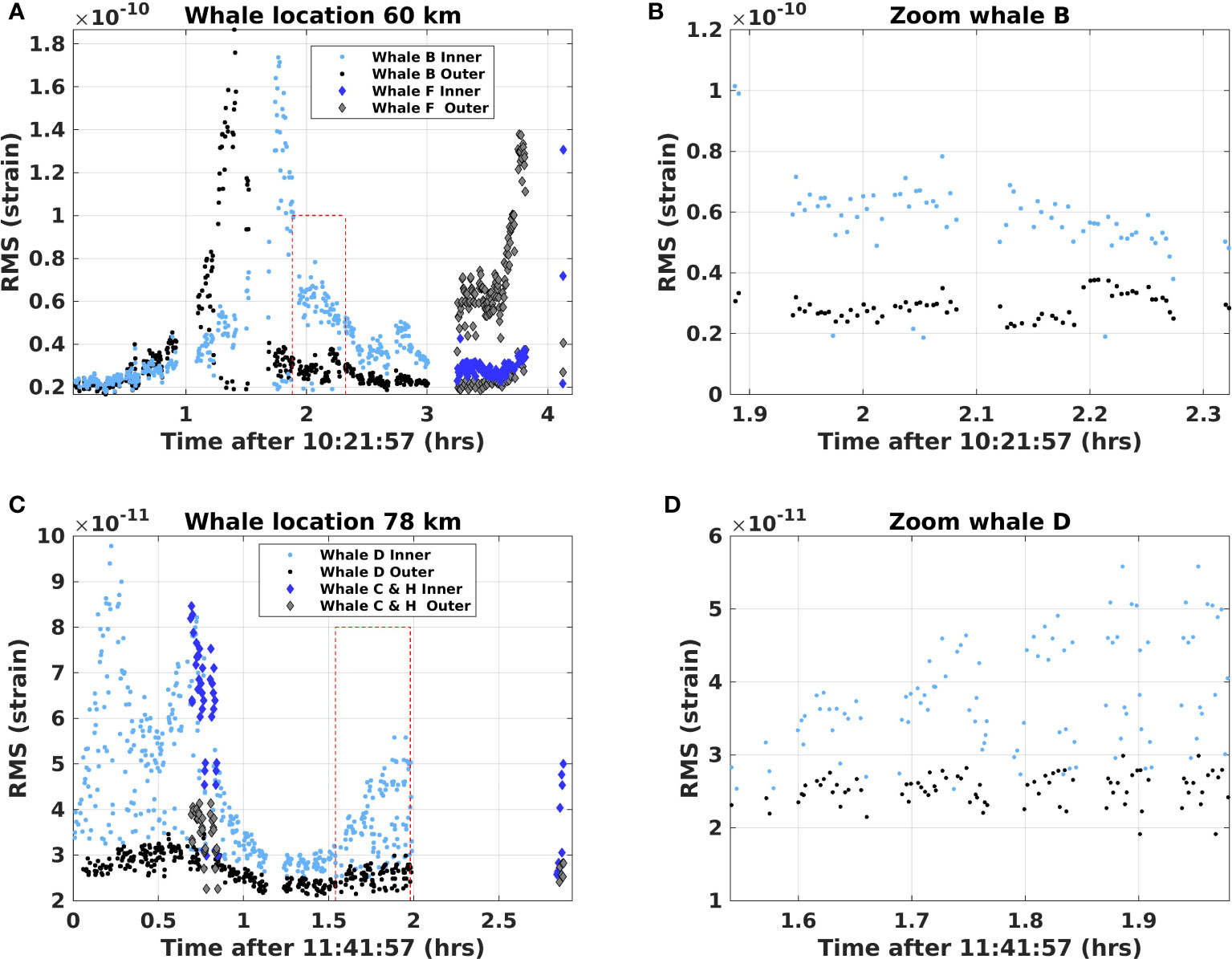
Figure 6 Observed RMS amplitudes of fin whale vocalizations in whale locations 60 km and 78 km (see Figure 5) computed by a rectangular window around the calls. (A, C) All RMS levels from the vocalizations in the respective locations. (B, D) Zoomed-in versions to illustrate periods with whale calls and the inter-series intervals.

We evaluated an empirical DAS detection range following Section 3.6, every 10 min, for all whale tracks. The detection range is represented as white dashed lines in Figure 5A. The obtained range does not monotonically decrease with fiber distance as whale track (D) at 80 km shows a longer range, 9.4 km, compared to, e.g., whale track (H) at 60 km with a range of 6.0 km. This suggests that other effects, such as coupling or the sediment properties, play a role or that the whales we observed at 80 km produced higher intensity calls than the whales at 60 km. This is not uncommon, e.g., Garcia et al. (2019) observed a significant variation in call levels and estimated fin whale sound intensity levels along the Norwegian coast to range from $186.3\pm 7.1$ to $195.8\pm 4.4$ dB. Moreover, whale (E) displays the lowest range (2.4 km). The large difference for whale (E) is believed to mainly be due to the increased background noise level at the location.

4.3 Fin whale individual characteristics

Over the $5.1$ h of analyzed data, five fin whale tracks were analyzed over a minimum of 45 min, providing insight on a few critical measurements for the species at the individual scale, based on a male 20 Hz song. We analyzed the sounds associated with each fin whale trajectory, reporting the total number of calls, average ICI, average ISI, and average swim speed in Table 1. Averages are associated with their standard deviation denoted by the ± symbol. Note that we excluded the first and last call series in each track as it is not clear if they contain a complete set of vocalizations.

TABLE 1

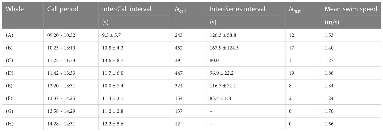
Table 1 Information on the different whale tracks, displaying the call period, the inter-call intervals, the inter-series interval, the mean swim speed and the number of calls during the different intervals.

Blue whale song is geographically distinct with differences in call time-frequency characteristics and repetition [ICI and ISI; McDonald et al. (2006)]. Our description of fin whale song follows Watkins et al. (1987), where a call series is defined as a group of at least five fin whale vocalizations, ICI corresponds to the time stretch between two consecutive 20 Hz calls that are $<60$ s, and ISI when the call interval is longer. Intervals are measured on a spatio-temporal representation of the signals, where the reference timings are picked along the same channel. Note also that the interrogator calibration break interval (11:13 to 11:23) was neither included in the ICI nor the ISI estimations.

While peak frequencies are fairly stable for fin whales, the most regionally-distinctive parameter is the ICI, e.g., Delarue et al. (2009) used ICIs in the North East Atlantic for stock differentiation. ICIs were found between 9.3 and 13.8 s, aligning with reports of systematically shorter ICIs in the Barents sea, measured post-2017 close to ≃10 s (Romagosa et al., 2022). Focusing only on the tracks with more than five observed ISI, we denote that the smallest interval was computed for whale (D; 96.9 s) and the longest for whale (B; 167.9 s), consistent with ISI reported by Watkins et al. (1987). ISIs varied substantially along track (B) with a standard deviation of 124.5 s, whereas whale D had the smallest ISI deviation of 22.2 s.

The BF uses 3–4 vocalizations to estimate swim direction. We found swim speeds between 1 and 3 m/s, with “instant” horizontal speeds between 1.24 m/s and $1.86$ m/s (4.5–6.7 km/h). It is consistent with previously-reported fin whale swim speeds of 1.2–3.9 m/s during vocal activity (McDonald et al., 1995; Clark et al., 2019), generally lower than cruising speeds (Lydersen et al., 2020).

5 Discussion

5.1 Localization error

We used the known ship’s GPS associated with the air gun data to evaluate the GS and BF localization errors. The distance between the ship’s GPS position and the source was compensated by moving the logged source position from the GPS 10 m behind the ship following the known track. However, this is only a partial solution as the source will drift with abrupt changes in ship’s heading and with variations in local conditions, e.g., ocean currents and weather, during the acquisition. These variations could introduce some errors into the airgun position estimate.

Comparing the errors in airgun position estimation to the errors in the telecommunication cable coordinates and the time of arrival picks, we consider the error in the airgun shot location as negligible. The fiber track locations were logged while the cables were trenched into the substrata. Moreover, the DAS system saves data into channels related to the distance the laser has traveled along the cable, which must be calibrated to the known telecommunication cable coordinates. As we know the coordinates along the fiber track, we can compute distances along the cable that roughly correspond to the distances logged by the interrogator equipment. However, the cable is not necessarily fully stretched; hence the distance calculated from the known fiber track position could deviate from the distances logged by the interrogator unit. Using the geo-referenced shot position, a future study could focus on developing an inversion procedure to match the distances that the interrogator logs with the known cable positions and quantify the potential errors.

First arrival times were manually picked on conditioned spatio-temporal representations of the data. We identify manual time-picking as a source of error directly related to the apparent SNR. For a specific DAS configuration and stable source characteristics as in the air gun example, the SNR will change with the distance between the source and the fiber (both on the horizontal plane and with changes in the water column depth), the ambient noise but also, changes in DAS recording capabilities all along the fiber.

Considering the configuration of (1) a pelagic sound source in the [5-45] Hz (air gun) and [15-25] Hz (fin whale) frequency band, (2) bottom-mounted receivers and, (3) a constrained detection range of 9.4 km we assumed a constant sound speed (and, therefore, straight ray travel time; see equation 1) to limit the computational costs of the localization methods. When estimating the air gun track, we tested various sound speeds and found the value with the lowest error to be 1440 m/s. The obtained sound speed agrees with average values given for sea-water at 4-6°C, which are typical for Svalbard (Timmermans and Labe, 2022), also used in previous studies of Arctic waters (see, e.g., Gavrilov and Mikhalevsky (2006)). We carried out a simple test to see the change in average errors between the known shot position and the estimated track. Increasing the sound speed by 25 and 50 m/s produced a 16 and 31 m increase in average errors. In the event longer detection ranges were available or to reduce the obtained 100 m localization error, 3D propagation modeling might be necessary to account for the complex bathymetry in fjord environments (e.g., using BELLHOP (Ocean-Acoustic-Library, 2022)), as highlighted in neighboring fjords (Richard et al., 2023).

The typical depth range for fin whale vocalizations is between 15 and 30 m (Oleson et al., 2014). We investigated a similar depth range using the air gun data to quantify the errors related to using a fixed source depth by changing the source depth of the air gun in the localization algorithms to 20 m while keeping the sound speed constant at 1440 m/s. The BF localization errors deviate less than 1 m, whereas the GS deviates with just over 1 m. The very low deviations in errors are likely because we are investigating depth variation well below the location accuracy.

5.2 Comparison of the localization methods

The two localization algorithms provide similar results for both the air gun and the whale vocalization and show similar localization errors of 100 m. For the air gun track, the GS showed a smaller error than the BF (Figure 2), whereas, for the whale tracks, the GS generated positions that are more scattered than the BF (Figure 5). This is attributed to the BF incorporating knowledge of previous locations, whereas the GS location estimates are independent for each vocalization.

Because of the manual first time of arrival picking, the methods from raw data to a position, swim speed and direction, and ultimately the tracks still need to be fully automated. The manual picks were limited by the SNR of the observed signal, which translated into a minimum received RMS strain of $0.2\times {10}^{-10}$ on Figure 6 which in turn limited the detection and localization range to a maximum offset of 9.4 km from the fiber, for both methods. For fin whales’ 20 Hz song, the arrival times selection could be automated, e.g., by a time-frequency matched filter (also known as spectrogram correlation; Mellinger and Clark (2000)) or by adapting recent advances in machine learning and convolutional neural networks to analyze the large amount of DAS-collected data and detect whale calls with high accuracy (Shiu et al., 2020). Automating the time of arrival picking could help extend the localization’s spatial reach and potentially reduce the localization error.

The implementations of the algorithms used to find the tracks in this paper are computationally different. The GS is a brute force algorithm that finds arrival times for grid points over a pre-defined area and uses, for instance, 1.9 s to locate one air gun shot. Conversely, the BF is more computationally efficient and uses 0.15 s to locate one seismic shot. These computational times denote the applicability and potential for near-real-time whale tracking. The computational efficiency of the methods strongly depends on the computer used, the processing unit (CPU vs. GPU), the programming language, and the algorithms’ efficiency, and it can be optimized for better performance.

Under the considerations of near-real-time tracking, the BF stands out as the most complete method as it estimates the heading and speed of the whales in addition to its geographical position. In contrast, the GS only estimates the geographical position of the whale call. However, it is a global optimization method with few assumptions in the inversion procedure. It is limited by the grid spacing, the size of the area covered by grid points, and the complexity of travel times calculations. The latter limitation is also valid for the BF. Additionally, it computes the misfit function for the whole grid area, which might show features in the objective function not captured by the BF. This can serve as a comparison to the BF (as done here) to find local minima in the grid area or provide an accurate starting model for the BF (or a similar local optimization method dependent on an accurate initial model). For example, when one cable is used, it will highlight the left-right ambiguity problem in the misfit function. The contours from the GS position, as depicted in Figure 2D, align well with the various error ellipses from the BF, which indicates that the Gaussian approximation used in the BF is a good approximation for situations like those studied here.

5.3 Implication of DAS-based localization for whale conservation

Telecommunication cables are available worldwide, and most new cables have more optical fibers than required to create redundancy. These could be repurposed to create distributed sensors from their onshore termination point to the first repeater. However, there are a limited number of places where two parallel fibers are laid a few km apart, as in this study. Even with one fiber, we can still detect and estimate the direction (with a left/right ambiguity) of vocalizing whales, with range inferred by, e.g., the received levels and the directional ambiguity perhaps broken by an asymmetry in the bathymetry (see, e.g., Bouffaut et al. (2022)). However, additional work is needed to quantify the instrument response of DAS, its directivity, and sensitivity at higher frequencies to understand which species can be monitored with this technology and under what circumstances.

The localization accuracy of the two methods presented in this work has been shown to be ≃100 m while offering the possibility to localize whales over a ≃1800 km² area (considering whales being detected at a distance of up to 95 km from the interrogators in Longyearbyen, with a detection range of ≃9.4 km). This combination of spatial coverage, relatively low infrastructural investment, and potential for real-time monitoring could bring great value to a range of coastal conservation applications.

For example, driven by the North Atlantic right whale case, several acoustic-based methods are being developed or applied to mitigate the risk of ship strikes (e.g., Gervaise et al. (2021); Baumgartner et al. (2019)). For this application, real-time methods are essential, and the obtained 100 m accuracy compares well with current practices (Hendricks et al., 2019). Such a collision management system is becoming increasingly important in the Arctic, where the decrease in sea-ice coverage opens up new shipping routes that might impact previously untouched whale habitats. At the same time, climate change is likely causing whales to change their habitat use and migration behavior. By automating the tracking procedure presented here, it would be possible to produce near-real-time tracks of whales with species identification, swim speed, and direction. At the very least, this information could be used to inform local management and stakeholders of whale presence and movement in a timely manner and at a very fine spatial resolution, supporting them to take appropriate mitigation measures. Furthermore, detailed information on whale locations and behavior would support science-based decisions and the management of conservation areas where anthropogenic activities should be kept at a minimum. Svalbard is a known summer feeding ground for baleen whales (Storrie et al., 2018), and mapping the common or active feeding areas is important. A final possibility is to find information on how whales respond to the changing marine ecosystem in the Arctic, induced by climate change, which has already been shown to alter baleen whale behavior (Moore et al., 2019). A global effort is needed to obtain such information, in which DAS systems can provide detailed information through high spatial and temporal sampling.

6 Conclusion

Examining five hours of data from two fiber-optic telecommunication cables, we have detected 1808 fin whale vocalizations. A subset of these data has been used to track eight whales during this period, with up to four being tracked simultaneously at a detection range from the cable of up to 9.4 km. This capability opens up new possibilities for detailed mapping of the presence and location of whales over large areas (at least 60 km long and$\simeq$20 km wide) over long periods, in near real-time. The simultaneous tracking of multiple whales also has the potential to provide new insights into the behavior and interaction between whales along a corridor up to ≃9.4 km on either side of the cable. Using shots from a single air gun towed behind a ship, we were able to calibrate our two localization estimators (a grid search and a Bayesian filter) with deterministic signals of similar source level to fin whale calls and found both methods to be computationally efficient and accurate to ≃100 m. Using two fiber cables, separated by a few km, breaks the symmetry of a single straight-line array, resolving the usual left-right ambiguity. The capabilities demonstrated here establish the potential for a near-real-time whale tracking capability that could be applied anywhere in the world where there are whales and fiber-optic cables. Coupled with ship detection, using a similar approach and/or with fused data from other sources such as AIS, a real-time collision avoidance system could be developed to reduce ship strikes.

Data availability statement

The original contributions presented in the study are publicly available. This data can be found here: https://doi.org/10.18710/Q8OSON.

Ethics statement

Ethical review and approval were not required for the animal study because it was conducted by remote sensing using passive acoustics without any kind of contact, interactions or disturbances of the animals.

Author contributions

RR wrote the manuscript with support from JE, LB and JP, which was read and approved by all co-authors. RR carried out the acoustic analysis; RR and JE developed and conducted the whale tracking; RR produced the results shown in the manuscript, interpreted together with JE, LB, ML, JP, and KT. ML, RR, SJ, FS, JJ, OS, SW, VO, and AW, planned the experiment, and RR, JJ, and FS collected the DAS data. ML, VO, and AW provided the OptoDAS interrogator used. BR and TJ conducted the air gun experiment. All authors contributed to the article and approved the submitted version.

Funding

RR and KT are funded by the Geophysics and Applied Mathematics in Exploration and Safe production Project (GAMES) at NTNU (Research Council of Norway; Grant No. 294404). We acknowledge support from the Centre for Geophysical Forecasting - CGF (grant no. 309960). The acquisition of the data was financed by CGF.

Conflict of interest

Author KT was employed by PTT Exploration and Production Public Company Limited.

The remaining authors declare that the research was conducted in the absence of any commercial or financial relationships that could be construed as a potential conflict of interest.

Publisher’s note

All claims expressed in this article are solely those of the authors and do not necessarily represent those of their affiliated organizations, or those of the publisher, the editors and the reviewers. Any product that may be evaluated in this article, or claim that may be made by its manufacturer, is not guaranteed or endorsed by the publisher.

Supplementary material

The Supplementary Material for this article can be found online at: https://www.frontiersin.org/articles/10.3389/fmars.2023.1130898/full#supplementary-material

References

Abadi S. H., Tolstoy M., Wilcock W. S. (2017). Estimating the location of baleen whale calls using dual streamers to support mitigation procedures in seismic reflection surveys. PloS One 12, e0171115. 564. doi: 10.1371/journal.pone.0171115

CrossRef Full Text | Google Scholar

Ahonen H., Stafford K. M., de Steur L., Lydersen C., Wiig Ø., Kovacs K. M. (2017). The underwater soundscape in western fram strait: Breeding ground of spitsbergen’s endangered bowhead whales. Mar. Pollut. Bull. 123, 97–112. doi: 10.1016/j.marpolbul.2017.09.019

PubMed Abstract | CrossRef Full Text | Google Scholar

Ahonen H., Stafford K. M., Lydersen C., Berchok C. L., Moore S. E., Kovacs K. M. (2021). Interannual variability in acoustic detection of blue and fin whale calls in the northeast Atlantic high Arctic between 2008 and 2018. Endangered Species Res. 45, 209–224. doi: 10.3354/esr01132

CrossRef Full Text | Google Scholar

Baumgartner M. F., Bonnell J., Van Parijs S. M., Corkeron P. J., Hotchkin C., Ball K., et al. (2019). Persistent near real-time passive acoustic monitoring for baleen whales from a moored buoy: System description and evaluation. Methods Ecol. Evol. 10, 1476–1489. doi: 10.1111/2041-210X

CrossRef Full Text | Google Scholar

Bouffaut L., Landrø M., Potter J. R. (2021). Source level and vocalizing depth estimation of two blue whale subspecies in the western Indian ocean from single sensor observations. J. Acoustical Soc. Am. 149 (6), 4422–4436. doi: 10.1121/10.0005281

CrossRef Full Text | Google Scholar

Bouffaut L., Taweesintananon K., Kriesell H. J., Rørstadbotnen R., Potter J. R., Landrø M., et al. (2022). Eavesdropping at the speed of light: Distributed acoustic sensing of baleen whales in the Arctic. Front. Mar. Sci. 9. doi: 10.3389/fmars.2022.901348

PubMed Abstract | CrossRef Full Text | Google Scholar

Clark C. W., Gagnon G. J., Frankel A. S. (2019). Fin whale singing decreases with increased swimming speed. R. Soc. Open Sci. 6, 180525. doi: 10.1098/rsos.180525

PubMed Abstract | CrossRef Full Text | Google Scholar

Comiso J. C., Parkinson C. L., Gersten R., Stock L. (2008). Accelerated decline in the Arctic sea ice cover. Geophysical Res. Lett. 35. doi: 10.1029/2007GL031972

CrossRef Full Text | Google Scholar

Cummings W. C., Thompson P. O. (1971). Underwater sounds from the blue whale, balaenoptera musculus. J. Acoustical Soc. Am. 50, 1193–1198. doi: 10.1121/1.1912752

CrossRef Full Text | Google Scholar

Delarue J., Todd S. K., Van Parijs S. M., Di Iorio L. (2009). Geographic variation in northwest atlantic fin whale (balaenoptera physalus) song: Implications for stock structure assessment. J. Acoustical Soc. Am. 125, 1774–1782. doi: 10.1121/1.3068454

CrossRef Full Text | Google Scholar

Dou S., Lindsey N., Wagner A. M., Daley T. M., Freifeld B., Robertson M., et al. (2017). Distributed acoustic sensing for seismic monitoring of the near surface: a traffic-noise interferometry case study. Sci. Rep. 7, 1–12. doi: 10.1038/s41598-017-11986-4

PubMed Abstract | CrossRef Full Text | Google Scholar

Eidsvik J., Hokstad K. (2006). Positioning drill-bit and look-ahead events using seismic traveltime data. Geophysics 71, F79–F90. doi: 10.1190/1.2212268

CrossRef Full Text | Google Scholar

Garcia H. A., Zhu C., Schinault M. E., Kaplan A. I., Handegard N. O., Godø O. R., et al. (2019). Temporal–spatial, spectral, and source level distributions of fin whale vocalizations in the norwegian sea observed with a coherent hydrophone array. ICES J. Mar. Sci. 76, 268–283. doi: 10.1093/598icesjms/fsy127

CrossRef Full Text | Google Scholar

Gavrilov A. N., Mikhalevsky P. N. (2006). Low-frequency acoustic propagation loss in the arctic ocean: Results of the arctic climate observations using underwater sound experiment. J. Acoustical Soc. Am. 119, 3694–3706. doi: 10.1121/1.2195255

CrossRef Full Text | Google Scholar

Gervaise C., Simard Y., Aulanier F., Roy N. (2021). Optimizing passive acoustic systems for marine mammal detection and localization: Application to real-time monitoring north atlantic right whales in gulf of st. lawrence. Appl. Acoustics 178, 107949. doi: 10.1016/j.apacoust.2021.107949

CrossRef Full Text | Google Scholar

Greene C. H., Pershing A. J. (2004). Climate and the conservation biology of north Atlantic 606 right whales: the right whale at the wrong time? Front. Ecol. Environ. 2, 29–34. doi: 10.1890/1540-9295(2004)002[0029:CATCBO]2.0.CO;2

CrossRef Full Text | Google Scholar

Hagen J. O., Liestøl O., Roland E., Jørgensen T. (1993). Glacier atlas of Svalbard and Jan mayen 129, 1–141. (Norsk Polarinstitutt Oslo).

Google Scholar

Hamilton C. D., Lydersen C., Aars J., Biuw M., Boltunov A. N., Born E. W., et al. (2021). Marine mammal hotspots in the Greenland and barents seas. Mar. Ecol. Prog. Ser. 659, 3–28. 612. doi: 10.3354/meps13584

CrossRef Full Text | Google Scholar

Harcourt R., van der Hoop J., Kraus S., Carroll E. L. (2019). Future directions in eubalaena spp.: comparative research to inform conservation. Front. Mar. Sci. 5, 530. doi: 10.3389/fmars.2018.00530

CrossRef Full Text | Google Scholar

Hartog A. H. (2017). An introduction to distributed optical fibre sensors. 1 edn (Boca Raton, FL: CRC Press). doi: 10.6171201/9781315119014

CrossRef Full Text | Google Scholar

Havskov J., Ottemoller L. (2010). Routine data processing in earthquake seismology: With sample data, exercises and software (Springer Science & Business Media). 347

Google Scholar

Hendricks B., Wray J. L., Keen E. M., Alidina H. M., Gulliver T. A., Picard C. R. (2019). Automated localization of whales in coastal fjords. J. Acoustical Soc. America 146, 4672–4686. doi: 10.1121/1.5138125

CrossRef Full Text | Google Scholar

Hoschle C., Cubaynes H. C., Clarke P. J., Humphries G., Borowicz A. (2021). The potential of satellite imagery for surveying whales. Sensors 21, 963. doi: 10.3390/s21030963

PubMed Abstract | CrossRef Full Text | Google Scholar

IPCC (2022). “Summary for policymakers,” in Climate change 2022: Mitigation of climate change (Cambridge, UK and New York, NY, USA: Cambridge University Press). Intergovernmental Panel on Climate Contribution: Contribution from working Group III to the Sixth Assessment Report.

Google Scholar

Jaskolski M. W. (2021). For human activity in Arctic coastal environments–a review of selected interactions and problems. Miscellanea Geographica 25, 127–143. doi: 10.2478/mgrsd-2020-0036

CrossRef Full Text | Google Scholar

Klinck H., Nieukirk S. L., Mellinger D. K., Klinck K., Matsumoto H., Dziak R. P. (2012). Seasonal presence of cetaceans and ambient noise levels in polar waters of the north Atlantic. J. Acoustical Soc. America 132, EL176–EL181. doi: 10.1121/1.4740226

CrossRef Full Text | Google Scholar

Landrø M., Bouffaut L., Kriesell H. J., Potter J. R., Rørstadbotnen R. A., Taweesintananon K., et al. (2022). Sensing whales, storms, ships and earthquakes using an Arctic fibre optic cable. Sci. 635 Rep. 12, 1–10. doi: 10.1038/s41598-022-23606-x

CrossRef Full Text | Google Scholar

Lavery T. J., Roudnew B., Seymour J., Mitchell J. G., Smetacek V., Nicol S. (2014). Whales sustain fisheries: blue whales stimulate primary production in the southern ocean. Mar. Mammal Sci. 30, 638 888–904. doi: 10.1111/mms.12108

CrossRef Full Text | Google Scholar

Lindsey N. J., Martin E. R., Dreger D. S., Freifeld B., Cole S., James S. R., et al. (2017). Fiber optic network observations of earthquake wavefields. Geophysical Res. Lett. 44, 11–792. 641. doi: 10.1002/2017GL075722

CrossRef Full Text | Google Scholar

Lydersen C., Vacquie-Garcia J., Heide-Jørgensen M. P., Øien N., Guinet C., Kovacs K. M. (2020). Autumn movements of fin whales (Balaenoptera physalus) from Svalbard, Norway, revealed by satellite 644 tracking. Sci. Rep. 10, 1–13. doi: 10.1038/s41598-020-73996-z

PubMed Abstract | CrossRef Full Text | Google Scholar

Matsumoto H., Araki E., Kimura T., Fujie G., Shiraishi K., Tonegawa T., et al. (2021). Detection of hydroacoustic signals on a fiber-optic submarine cable. Sci. Rep. 11, 1–12. doi: 10.1038/647s41598-021-82093-8

PubMed Abstract | CrossRef Full Text | Google Scholar

Maturilli M., Herber A., Konig-Langlo G. (2013). Climatology and time series of surface meteorology in ny-alesund, Svalbard. Earth System Sci. Data 5, 155–163. doi: 10.5194/essd-5-155-2013

CrossRef Full Text | Google Scholar

McDonald M. A., Fox C. G. (1999). Passive acoustic methods applied to fin whale population density estimation. J. Acoustical Soc. Am. 105, 2643–2651. doi: 10.1121/1.426880

CrossRef Full Text | Google Scholar

McDonald M. A., Hildebrand J. A., Webb S. C. (1995). Blue and fin whales observed on a seafloor array in the northeast pacific. J. Acoust. Soc Am. 98, 712–721. doi: 10.1121/1.413565

PubMed Abstract | CrossRef Full Text | Google Scholar

McDonald M. A., Mesnick S. L., Hildebrand J. A. (2006). Biogeographic characterization of 655 blue whale song worldwide: using song to identify populations. J. Cetacean Res. Manage. 8, 55–65. doi: 10.47536/jcrm.v8i1.702

CrossRef Full Text | Google Scholar

Mellinger D. K., Clark C. W. (2000). Recognizing transient low-frequency whale sounds 658 by spectrogram correlation. J. Acoustical Soc. Am. 107, 3518–3529. doi: 10.1121/1.429434

CrossRef Full Text | Google Scholar

Mestayer J., Cox B., Wills P., Kiyashchenko D., Lopez J., Costello M., et al. (2011). “Field trials of distributed acoustic sensing for geophysical monitoring,” in Seg technical program expanded abstracts 2011 (Society of Exploration Geophysicists), 4253–4257. doi: 10.1190/1.3628095

CrossRef Full Text | Google Scholar

Moore S. E., Haug T., V´ıkingsson G. A., Stenson G. B. (2019). Baleen whale ecology in arctic and subarctic seas in an era of rapid habitat alteration. Prog. Oceanography 176, 102118. doi: 10.1016/j.pocean.2019.05.010

CrossRef Full Text | Google Scholar

Nordli Ø., Przybylak R., Ogilvie A. E., Isaksen K. (2014). Long-term temperature trends and variability on spitsbergen: the extended Svalbard airport temperature series 1898–2012. Polar Res. 33, 21349. doi: 10.3402/polar.v33.21349

CrossRef Full Text | Google Scholar

Nowacek D. P., Christiansen F., Bejder L., Goldbogen J. A., Friedlaender A. S. (2016). Studying cetacean behaviour: new technological approaches and conservation applications. Anim. Behav. 120, 235–244. doi: 10.1016/j.anbehav.2016.07.019

CrossRef Full Text | Google Scholar

Ocean-Acoustic-Library (2022) Acoustic toolbox (Accessed 2023-02-12). Dataset.

Google Scholar

Oleson E. M., Sirovic A., Bayless A. R., Hildebrand J. A. (2014). Synchronous seasonal change in fin whale song in the north pacific. PloS One 9, e115678. doi: 10.1371/journal.pone.0115678

PubMed Abstract | CrossRef Full Text | Google Scholar

Papp B., Donno D., Martin J. E., Hartog A. H. (2017). A study of the geophysical response of distributed fibre optic acoustic sensors through laboratory-scale experiments. Geophysical Prospecting 65, 1186–1204. doi: 10.1111/1365-2478.12471

CrossRef Full Text | Google Scholar

Rørstadbotnen R. A., Landrø M., Taweesintananon K., Bouffaut L., Potter J. R., Johansen S. E., et al. (2022). “Analysis of a local earthquake in the Arctic using a 120 KM long fibre-optic cable,” in 83rd EAGE annual conference & exhibition (European association of geoscientists & engineers), vol. 2022 of conference proceedings, 1–5. doi: 10.3997/2214-4609.202210404

CrossRef Full Text | Google Scholar

Richard G., Mathias D., Collin J., Chauvaud L., Bonnel J. (2023). Three-dimensional anthropogenic underwater noise modeling in an arctic fjord for acoustic risk assessment. Mar. pollut. Bull. 187, 680 114487. doi: 10.1016/j.marpolbul.2022.114487

CrossRef Full Text | Google Scholar

Rivet D., de Cacqueray B., Sladen A., Roques A., Calbris G. (2021). Preliminary assessment of ship detection and trajectory evaluation using distributed acoustic sensing on an optical fiber telecom cable. J. Acoustical Soc. America 149, 2615–2627. doi: 10.1121/10.0004129

CrossRef Full Text | Google Scholar

Romagosa M., Nieukirk S., Cascao I., Marques T. A., Dziak R., Royer J.-Y., et al. (2022). Fin whale singalong: evidence of song conformity. bioRxiv, 2022–2010. MiriamRomagosa doi: 10.1101/2022.10.05.510968

CrossRef Full Text | Google Scholar

Roman J., Estes J. A., Morissette L., Smith C., Costa D., McCarthy J., et al. (2014). Whales as marine ecosystem engineers. Front. Ecol. Environ. 12, 377–385. doi: 10.1890/130220

CrossRef Full Text | Google Scholar

Sarkka S. (2013). Bayesian Filtering and smoothing (Cambridge university press).

Google Scholar

Schuler T. V., Kohler J., Elagina N., Hagen J. O. M., Hodson A. J., Jania J. A., et al. (2020). Reconciling Svalbard glacier mass balance. Front. Earth Sci. 8. doi: 10.3389/feart.2020.00156

CrossRef Full Text | Google Scholar

Shiu Y., Palmer K., Roch M. A., Fleishman E., Liu X., Nosal E.-M., et al. (2020). Deep neural networks for automated detection of marine mammal species. Sci. Rep. 10, 607. doi: 10.1038/697s41598-020-57549-y

PubMed Abstract | CrossRef Full Text | Google Scholar

Sirovic A., Williams L. N., Kerosky S. M., Wiggins S. M., Hildebrand J. A. (2013). Temporal ´ separation of two fin whale call types across the eastern north pacific. Mar. Biol. 160, 47–57. 700. doi: 10.1007/s00227-012-2061-z

PubMed Abstract | CrossRef Full Text | Google Scholar

Stimpert A. K., DeRuiter S. L., Falcone E. A., Joseph J., Douglas A. B., Moretti D. J., et al. (2015). Sound production and associated behavior of tagged fin whales (Balaenoptera physalus) in the southern California bight. Anim. Biotelemetry 3, 1–12. doi: 10.1186/s40317-015-0058-3

CrossRef Full Text | Google Scholar

Storrie L., Lydersen C., Andersen M., Wynn R. B., Kovacs K. M. (2018). Determining the species assemblage and habitat use of cetaceans in the svalbard archipelago, based on observations from 2002 to 706 2014 (Norwegian Polar institute) 37 (1). doi: 10.1080/17518369.2018.1463065

CrossRef Full Text | Google Scholar

Stroeve J., Holland M. M., Meier W., Scambos T., Serreze M. (2007). Arctic Sea ice decline: Faster than forecast. geophysical research letters, (American geophysical union) 34 (9). doi: 10.1029/2007GL029703

CrossRef Full Text | Google Scholar

Taweesintananon K., Landrø M., Brenne J. K., Haukanes A. (2021). Distributed acoustic sensing for near-surface imaging using submarine telecommunication cable: A case study in the trondheimsfjord, Norway. Geophysics 86, B303–B320. doi: 10.1190/geo2020-0834.1

CrossRef Full Text | Google Scholar

Taweesintananon K., Landrø M., Potter J. R., Johansen S. E., Rørstadbotnen R. A., Bouffaut L., et al. (2023). Distributed acoustic sensing of ocean-bottom seismo-acoustics and distant storms: A case study from svalbard, norway. Geophysics 88, 1–65. doi: 10.1190/geo2022-0435.1

CrossRef Full Text | Google Scholar

Thode A. M., D’Spain G., Kuperman W. (2000). Matched-field processing, geoacoustic inversion, and source signature recovery of blue whale vocalizations. J. Acoustical Soc. America 107, 1286–1300. doi: 10.1121/1.428417. 5.

CrossRef Full Text | Google Scholar

Thomas P. O., Reeves R. R., Brownell J. R.L. (2016). Status of the world’s baleen whales. Mar. Mammal Sci. 32, 682–734. doi: 10.1111/mms.12281

CrossRef Full Text | Google Scholar

Thompson P. O., Findley L. T., Vidal O. (1992). 20-Hz pulses and other vocalizations of fin whales, b alaenopteraphysalus, in the gulf of California, Mexico. J. Acoustical Soc. America 92, 3051–3057. doi: 10.1121/1.404201

CrossRef Full Text | Google Scholar

Timmermans M. L., Labe Z. (2022) Sea Surface temperature (Accessed Accessed: 2022-01-13). Dataset.

Google Scholar

Townhill B. L., Reppas-Chrysovitsinos E., Suhring R., Halsall C. J., Mengo E., Sanders T., et al. (2022). Pollution in the Arctic ocean: An overview of multiple pressures and implications for ecosystem services. Ambio, 51 (2), 471–483. doi: 10.1007/s13280-021-01657-0

PubMed Abstract | CrossRef Full Text | Google Scholar

van Weelden C., Towers J. R., Bosker T. (2021). Impacts of climate change on cetacean distribution, habitat and migration. Climate Change Ecol. 1, 1009. doi: 10.1016/j.ecochg.2021.100009

CrossRef Full Text | Google Scholar

Waagaard O. H., Rønnekleiv E., Haukanes A., Stabo-Eeg F., Thingbø D., Forbord S., et al. (2021). Real-time low noise distributed acoustic sensing in 171 km low loss fiber. OSA Continuum 4, 688–701. doi: 10.1364/OSAC.408761. 731.

CrossRef Full Text | Google Scholar

Watkins W. A., Tyack P., Moore K. E., Bird J. E. (1987). The 20-Hz signals of finback whales (Balaenoptera physalus). J. Acoustical Soc. America 82, 1901–1912. doi: 10.1121/7341.395685

CrossRef Full Text | Google Scholar

Wilcock W. S. (2012). Tracking fin whales in the northeast pacific ocean with a seafloor seismic network. J. Acoustical Soc. America 132, 2408–2419. doi: 10.1121/1.4747017

CrossRef Full Text | Google Scholar

Wilcock W. S., Abadi S., Lipovsky B. P. (2023). Distributed acoustic sensing recordings of low-frequency whale calls and ship noise offshore central oregon. JASA Express Lett. 3, 026002. doi: 10.1121/10.0017104

PubMed Abstract | CrossRef Full Text | Google Scholar

Wuestefeld A., Greve S. M., Nasholm S. P., Oye V. (2018). Benchmarking earthquake location algorithms: A synthetic comparison. Geophysics 83, KS35–KS47. doi: 10.1190/geo2017-0317.1

CrossRef Full Text | Google Scholar

Yigit C. O., Gikas V., Alcay S., Ceylan A. (2014). Performance evaluation of short to long term GPS, GLONASS and GPS/GLONASS post-processed PPP. Survey Rev. 46, 155–166. doi: 10.1179/7431752270613Y.0000000068

CrossRef Full Text | Google Scholar