Distinct vertical behavior of key Arctic copepods following the midnight sun period in the East Siberian continental margin region, Arctic Ocean

Introduction

The diel vertical migration (DVM) of zooplankton is the largest natural daily movement of biomass on Earth, with organisms moving upward at dusk and downward at dawn (Lampert, 1989; Brierley, 2014). Changes in light conditions are considered to be the triggering and synchronizing factors of zooplankton DVM (Fortier et al., 2001; Pearre, 2003). Due to the strong seasonality of solar radiation energy, high latitudes have unique light regimes, including midnight sun and polar night periods, and therefore have limited periods in which distinctive days and nights occur (Daase et al., 2021). Data on zooplankton DVM during distinct day and night periods in high-latitude regions are still insufficient (Daase et al., 2008; Falk-Petersen et al., 2008; Wallace et al., 2010).

The western Arctic Ocean is an ecologically important region due to its high productivity (Blachowiak-Samolyk et al., 2006). This region has recently experienced a rapid decrease in sea ice extent (Rodrigues, 2008; Wood et al., 2015), which could significantly impact the marine environment, including ocean circulation, stratification, light penetration, and phytoplankton productivity (Pabi et al., 2008; Nishino et al., 2011). Such environmental changes may subsequently affect the distribution of zooplankton as secondary producers (Feng et al., 2018). Three key copepod species – Calanus glacialis, Calanus hyperboreus, and Metridia longa – account for 50–80% of the biomass of Arctic zooplankton (Mumm et al., 1998; Darnis et al., 2008). The vertical migration of these species not only supplies carbon from the surface to the benthic region in Arctic marine ecosystems (Kosobokova and Hirche, 2009; Forest et al., 2011; Sampei et al., 2012) but can also affect the distributions of their major predators, such as fish (Boreogadus saida, Mallotus villosus) and whales (Balaena mysticetus) (Benoit et al., 2010; Pomerleau et al., 2012; Hop and Gjøsæter, 2013; McNicholl et al., 2016). Therefore, it is important to accurately understand the vertical distributions of these key copepod species to gain insight into the interrelationships among organisms within the Arctic marine ecosystem.

Whether the key copepod species undergo DVM in summer and which migration-modulating factors affect this process remain open questions (Blachowiak-Samolyk et al., 2006; Wallace et al., 2010). Many studies have been conducted to explore the DVMs of key copepod species during the midnight sun period (Fortier et al., 2001; Blachowiak-Samolyk et al., 2006; Cottier et al., 2006; Rabindranath et al., 2011). Although DVM has been observed in key copepod species under continuous illumination conditions (Fortier et al., 2001; Rabindranath et al., 2011), opposite results have also been reported (Blachowiak-Samolyk et al., 2006). Falk-Petersen et al. (2008) noted that small light variations during the midnight sun period make it difficult to prove that zooplankton perform DVM. Daase et al. (2008) confirmed the non-DVM behavior of C. glacialis and C. hyperboreus as well as the DVM behavior of M. longa through net samplings conducted by dividing the entire water column into five depth intervals in the Svalbard region after the midnight sun period. The results showed that light conditions had a major influence on the DVM of M. longa; however, the vertical distribution ranges of the three copepod species were not determined due to coarse vertical and temporal sampling intervals. Additionally, the result was insufficient to confirm the possibility of DVM (short-range migration) in the two Calanus species at distances less than the net sampling depth intervals (Daase et al., 2008). Falk-Petersen et al. (2008) identified DVM in C. hyperboreus in the ice-edge region of Svalbard using acoustic and net sampling after the midnight sun period and found that light conditions and food influenced its DVM behavior. Their study confirmed the DVM of zooplankton through high-resolution acoustic backscatter (receiver signal strength indicator) observations. However, only a single frequency (120 kHz) was used for zooplankton DVM observation, and the acoustic backscatter range (-80 dB – -50 dB) used for acoustic analysis was only suitable for the detection of large (> 7 mm) copepods such as adult C. hyperboreus. While hydrographic conditions also critically impact the vertical distributions of zooplankton (Daase and Eiane, 2007; Blachowiak-Samolyk et al., 2008), only a few studies have explored the relationships between DVMs and hydrographic conditions for these key copepod species (Wallace et al., 2010; La et al., 2018).

In this context, the aim of this study was to investigate the DVM of key copepod species and identify the vertical distribution of each species in the East Siberian continental margin (ESCM) region, where few studies have previously been conducted after the midnight sun period. We also investigated marine environmental factors affecting the vertical distribution of key copepods. For this purpose, acoustic, biological, and oceanographic observations were carried out. These results contribute to a better understanding of the behaviors and functions of zooplankton in the rapidly changing Arctic Ocean.

Materials and methods

Study area

The ESCM region includes the northernmost continental shelf and slope of the East Siberian Sea and the West Chukchi Sea as well as parts of the Arlis Plateau, Chukchi Plateau, and Mendeleev Ridge in the Central Arctic Ocean (Niessen et al., 2013) (Figure 1). The bottom depth in this region ranges from 50 m to 2000 m, and the area exhibits a complex hydrographic structure as water masses originating in the North Pacific and North Atlantic converge with the Arctic water mass (Woodgate, 2013). Four major water mass structures have been identified in the study area (Linders et al., 2017): meltwater/runoff (MWR; salinity > 30 PSU and temperature < 2 °C; 30 < salinity < 31.5 PSU and temperature < -1 °C), Bering summer water (BSW; 30 < salinity < 33.3 PSU and -1 < temperature < 3 °C), remnant winter water (RWW; 31.5 < salinity < 35 PSU and -1.6 < temperature < -1 °C), and Atlantic water (AW; salinity > 33.3 PSU and temperature > -1 °C).

FIGURE 1

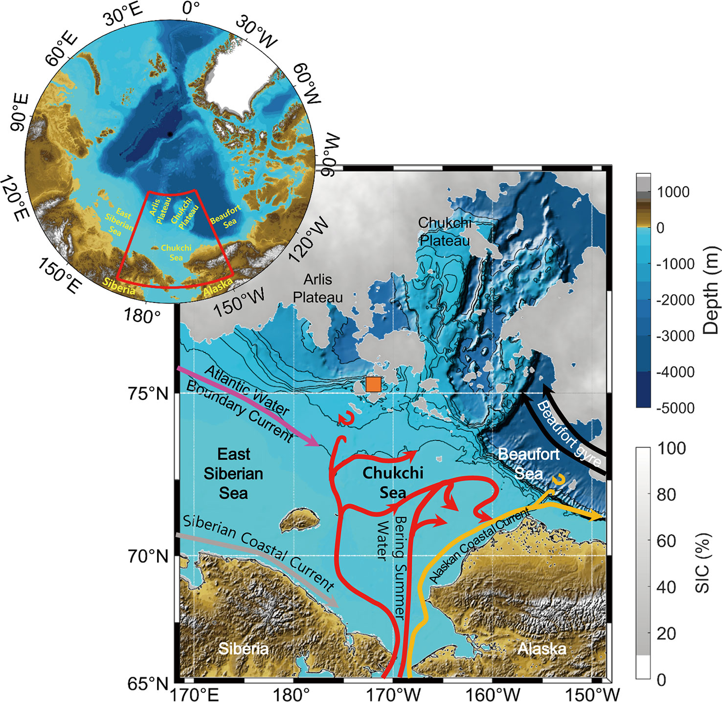
Figure 1 Bathymetric map of the ESCM region, with regional circulation patterns denoted as suggested by Pacini et al. (2019). The orange square presents the study area. The solid arrows represent flow pathways in the western Arctic Ocean. The red, orange, gray, magenta, and black arrows denote the Bering summer water, Alaskan Coastal Current, Siberian Coastal Current, Atlantic water, and Beaufort Gyre patterns, respectively. The gray shadow denotes sea ice concentrations derived from Advanced Microwave Scanning Radiometer 2 (AMSR2) satellite data (https://seaice.uni-bremen.de/sea-ice-concentration/amsre-amsr2) averaged from 11 to 30 August 2020.

Acoustic, biological, and oceanographic data collection

The study was carried out in the ESCM region aboard the icebreaker research vessel Araon from August 27 to 29, 2020, in local time (hereafter, all times are presented in local time). During this period, the vessel drifted approximately 41 km over bottom depths ranging from 495 to 635 m in an open-water environment, with a few drifting ice floes observed.

Acoustic backscatter (Sv, dB re 1 m^-1) data were continuously collected using an EK60 scientific echosounder (Simrad) operating at three frequencies (38, 120, and 200 kHz) during the survey period. The transceiver was set to a pulse length of 1.024 ms and a ping interval of 1 to 2 seconds. EK60 calibration values previously obtained under similar environmental conditions in the Ross Sea, Antarctica, were used for acoustic data analysis (Table 1).

TABLE 1

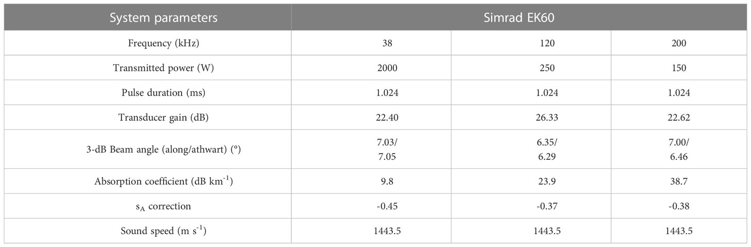
Table 1 Parameter settings of the scientific echosounder.

Vertical profiles of hydrographic variables, including temperature, salinity, density gradient, and fluorescence, were recorded using a portable conductivity-temperature-depth system (CTD; RBR, RBRconcerto) equipped with a fluorometer (Seapoint) sensor. The day and night measurements were performed during the highest and lowest sun elevations. Night-time and daytime CTD observations were performed at 00:25 h and at 13:15 h on 29 August, respectively. CTD casts were performed from the surface to 200 m according to the water depth where acoustic data analysis at a frequency of 200 kHz is possible. The mixed layer depth (MLD) is defined as the depth at which the density difference from the in situ density at 10 m is Δσ_θ = 0.03 (kg, m^-3) (Schneider and Müller, 1990). Because the fluorometer sensor was not calibrated, only relative values of chlorophyll a (chl-a) concentration (a proxy for phytoplankton biomass) are indicated.

To analyze the composition of the phytoplankton size classes, seawater was sampled at depths of 2, 10, 15, 20, 30, 47, 60, 80, and 100 m using a CTD/rosette equipped with 20-L PVC Niskin on 27 August. The seawater samples were sequentially filtered onto a Whatman GF/F filter (24 mm) and 20- and 2-μm membrane filters. Each filter was extracted in 90% acetone from 12 to 24 prior to chl-a concentration measurement using a fluorometer (Trilogy, Turner Designs).

Solar radiation was measured in real time at 10-second intervals using a downward shortwave measurement sensor (CMP11, Kipp and Zonen, Netherlands) installed on the research vessel. For light quantity analysis, the observed data were averaged at 10-minute intervals. The time period at which the light intensity exceeded 0 was defined as the daytime period (Jarolím et al., 2010).

The zooplankton community composition in the sound scattering layers (SSLs) was identified through repeated vertical sampling with a bongo net (330 µm mesh, mouth area of 0.28 m²). The number of bongo net deployments performed depended on the number of SSLs observed each day and night (Figure 2). Zooplankton were first collected in the SSLs located at the shallowest depth. The net and cod-end were thoroughly rinsed with ambient seawater after collection. At night, two SSLs were observed between the sea surface and 25 m and between 30 and 50 m. During the day, three SSLs were observed between the surface and 20 m, between 30 and 55 m, and between 100 and 135 m. All bongo nets were lowered 5 m deeper than the maximum depth of the target SSL. Zooplankton samples were immediately fixed with 5% neutral formalin before the abundance of each species was counted. For each net sample, 30 individuals of each key copepod species were randomly extracted, and their prosome lengths were measured to obtain the length-frequency distribution, which is a necessary metric for identifying the acoustic backscatter of key copepods. Because the prosome length of detectable copepods at a frequency of 200 kHz is at least 2 mm (Emery and Thomson, 2001), we randomly extracted dominant copepods with lengths larger than 2 mm.

FIGURE 2

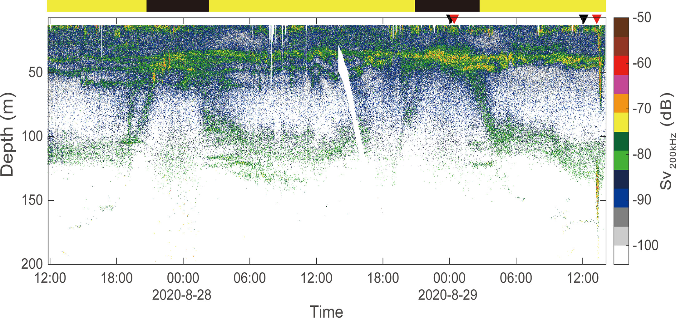
Figure 2 Sound scattering layers in the noise-removed echogram measured at 200 kHz. Three SSLs were observed: one between the surface and 20-m depth, one at depths of 30 to 55 m, and one at depths of 30 to 135 m. The black and red triangles on the upper margin mark the start time of each bongo net and CTD cast, respectively. The horizontal bar represents nighttime (black) and daytime (yellow).

Acoustic data processing

Acoustic data were processed and analyzed using Echoview 8 (Echoview Software Pty Ltd) and MATLAB (R2021a; Mathworks, Inc.) (Figure 3). Various noises (background noise, surface noise caused by air bubbles, nonbiological signals, and transient noise) within the raw data were removed using the methods of De Robertis and Higginbottom (2007) and Ryan et al. (2015) (Figures 3B, C). The acoustic backscatter of zooplankton was identified using the dB-difference method (Brierley et al., 1998) on the noise-processed data (Figures 3D–F). Acoustic backscatter in the range of 4 < Sv_{120-38 kHz} < 20 dB was identified as zooplankton (Kang et al., 2002). Then, the difference between the two frequencies (Sv_{200-120 kHz}) was applied to the 120- and 200-kHz filtered echograms to identify the dB difference characteristics of the zooplankton acoustic backscatter (Figure 3F).

FIGURE 3

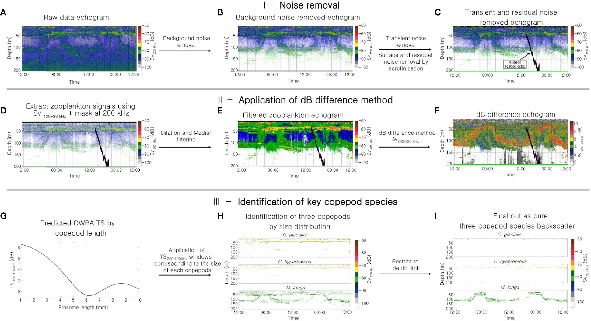
Figure 3 General outline of the multifrequency acoustic identification process of C. glacialis, C. hyperboreus and M. longa, comprising three steps. The irregular black shape (C) corresponds to an aliased seabed echo, also known as false bottom, detected and removed during the 38 kHz echogram.

Acoustic identification of the key copepod species

Acoustic backscatters of the key copepod species were identified by combining acoustic backscatter characteristics and the confirmed vertical distribution from the net surveys (Figures 3G–I). To determine the Sv_{200-120 kHz} window range required to identify acoustic backscatter of the key copepods, the acoustic backscatter characteristics of copepods along lengths (1–10 mm) at two frequencies (120 and 200 kHz) were predicted using the distorted-wave Born approximation (DWBA) model (Stanton and Chu, 2000; Demer and Conti, 2005) (Figure 3G). All of the DWBA model input parameters, except for shape, were referenced from the literature values. Acoustic scattering characteristics of zooplankton with similar classes can be predicted using a single shape of zooplankton through the DWBA model (Sakinan and Gücü, 2017; Gastauer et al., 2022). Thus, we digitized the shape of a 4.81 mm size of C. glacialis, employed it as a parameter for the DWBA model, and predicted the target strength of three key copepod species. The sound contrast (g) and density contrast (h), other parameters of the DWBA model, were set to 1.007 and 1.005, respectively (Smith et al., 2010), and the orientation distribution was set to N [90°, 30°] (Benfield et al., 2000). The minimum threshold (T_min) and maximum threshold (T_max) were determined and applied to acoustic identification (Figure 3H); these thresholds were calculated as the boundaries at the 95% confidence intervals in the respective acoustic scattering intensity distribution of the extracted species. For C. glacialis, the T_min and T_max values determined at a frequency of 120 kHz were -80 dB and -64 dB, respectively; the T_min and T_{max values} at 200 kHz were -78 dB and -63 dB, respectively. For C. hyperboreus, the T_min and T_max values derived at a frequency of 120 kHz were -83 dB and -71 dB, respectively; these values were -76 dB and -65 dB, respectively, at 200 kHz. For M. longa, the T_min and T_max values calculated at 120 kHz were -88 dB and -82 dB, respectively; the corresponding values were -82 dB and -75 dB, respectively, at a frequency of 200 kHz. The Sv_{200-120 kHz} window ranges of each key copepod species were determined by extracting the predicted DWBA model results corresponding to the length-frequency distribution of the measured key copepod species. The calculated Sv_{200-120 kHz} ranges for C. glacialis, C. hyperboreus, and M. longa were -0.1–7.3 dB, -0.7–4.0 dB, and 4.0–7.6 dB, respectively. By combining the threshold values and the Sv_{200-120 kHz} window ranges for each key copepod species, the acoustic backscatters of these species were identified (Figure 3H). The depth distribution information of the three species identified from the net surveys was used to identify their acoustic backscatters. The water depth ranges used to identify acoustic backscatter of key copepods were delineated to depths of 15–25 m and 25–60 m in the case of C. glacialis and C. hyperboreus, respectively. For the acoustic backscatter of M. longa, a limiting condition was applied in consideration of both the light intensity and net depth distribution. From the solar radiation analysis results, the nighttime hours corresponding to the first and second DVM cycles of M. longa were found to be 8:50–14:00 and 8:50–15:00, respectively. The water depth limit was set to 25–100 m to separate the acoustic backscatters of M. longa in the nighttime period corresponding to these two periods to include both the ascending and descending components. For the daytime hours, the water depth limit was set to 65–135 m. Finally, the identified acoustic backscatter of the three copepod species was clearly distinguished (Figure 3I).

Statistical analysis

A Pearson correlation analysis was performed to identify the marine environmental factors affecting the vertical distributions of C. glacialis, C. hyperboreus, and M. longa using MATLAB. For the one-to-one correlation analysis by water depth between the acoustic backscatter of the key copepod species and the marine environment measured by CTD, the CTD depth resolution was averaged at 0.2 m intervals, which is the same resolution as the acoustic data, and then used for statistical analysis. Significant differences were considered statistically significant at p < 0.01.

Results

Environmental conditions

Solar radiation exhibited a clear daily cycle during the study period (Figure 4). The sunrise and sunset times on 28 August were 02:36 and 20:16, respectively, while on 29 August, they were 02:43 and 20:09. (https://gml.noaa.gov/grad/solcalc/sunrise.html). The light intensities ranged between 0 and 268.5 (W m^-2), indicating a significant difference in light conditions between day and night during the observation periods.

FIGURE 4

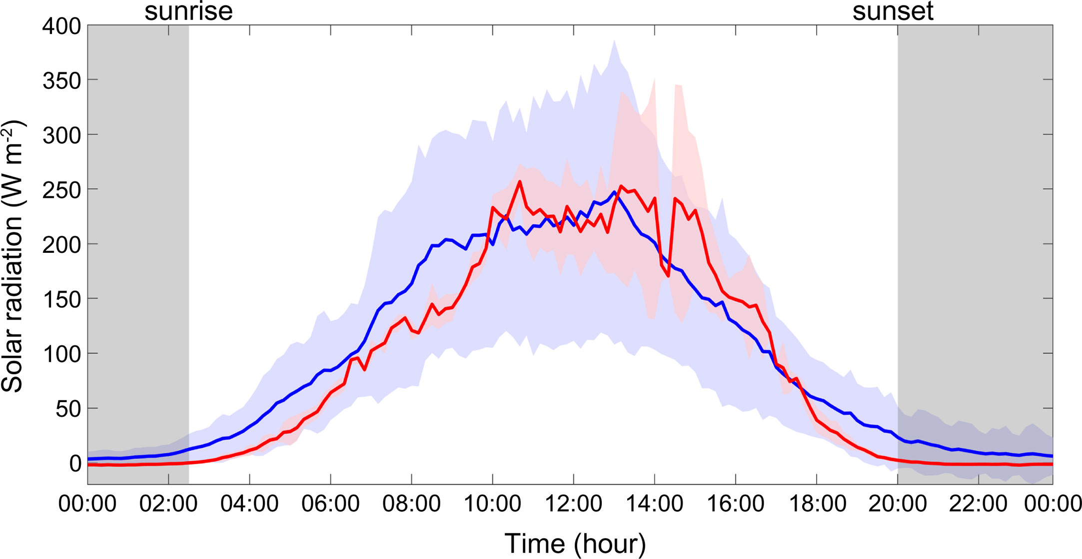
Figure 4 Hourly variations in daily solar radiation in August 2020. Solid blue and red lines indicate monthly mean and study period mean values, respectively.

The physical and biological properties of the water column showed similar profiles during the day and at night (Figure 5). The MLD was observed at 12.0 m and 11.7 m in the nighttime and daytime, respectively. Water temperature (-0.6 °C) and salinity (27.05 PSU) were constant from the surface to ~12 m and ranged from -0.6 to -0.9 °C and from 27.00 to 28.88 PSU between 12 and 18 m. Below this layer, the water temperature and salinity ranged from -1.5 to -0.9 °C and from 28.99 to 32.01 PSU between 18 and 47 m. In the depth range between 47 and 143 m, the water temperature varied between -1.5 and -1.1 °C, while the salinity continued to increase up to 34.29 PSU. The water temperature and salinity ranged between -1.1 and -0.2 °C and between 34.29 and 34.57 PSU, respectively, from 143 to 200 m. The density gradient showed peak values of 0.16 dρ/dz and 0.10 dρ/dz at depths of 19 m and 134 m, respectively, with relatively large density changes near these two depths (Figure 5C). The subsurface chlorophyll maximum (SCM) was observed at 38.6 m at night and at 39.5 m during the day (Figure 5D). The phytoplankton size classes showed a larger contribution of picophytoplankton (< 2 μm) at 2 and 30 m, while micro phytoplankton (> 20 μm) contributed to the majority at 47 m, where high fluorescence was observed (Figure 5D). Overall, the picophytoplankton decreased as the water depth increased, while the micro phytoplankton increased with depth.

FIGURE 5

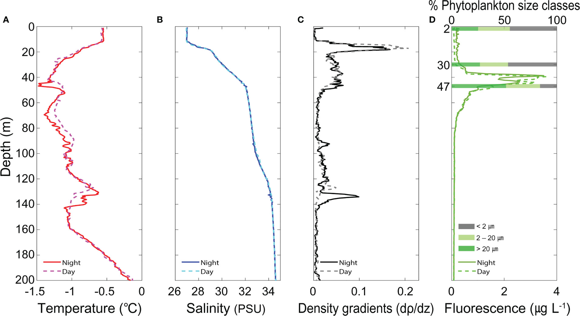
Figure 5 Vertical profiles of the (A) temperature, (B) salinity, (C) density gradient, and (D) fluorescence, along with the phytoplankton size classes (> 20, 2−20, and < 2 μm).

The water mass structure of the study area was divided into five categories based on Gong and Pickart (2015) and Linders et al. (2017) (Figure 6): late season meltwater, early season meltwater, remnant winter water, Bering summer water, and Atlantic water. Late season meltwater forms when sea ice thaws during the summer and supplies fresh water (Paquette and Bourke, 1981; Pacini et al., 2019), as observed from 1 to 24 m. Early season meltwater is highly saline due to the brine supplied by brine rejection during the formation of sea ice in the previous winter; this water mass also forms as water warms in the absence of clear dilution as summer approaches (Paquette and Bourke, 1979; Pacini et al., 2019). The early season meltwater was observed at depths between 24 and 42 m and showed higher water temperatures and higher salinity values than the late season meltwater. Remnant winter water forms in summer when winter water mixes with summer water or is warmed by solar heat (Gong and Pickart, 2015). The remnant winter water was observed in two water layers at depths between 42 and 116 m and between 142 and 160 m. The Bering summer water, a water mass originating from the central/western Bering Sea (Gong and Pickart, 2015), was observed at depths between 106 and 107 m. The Atlantic water, the most saline among the categories, was observed at depths between 116 and 142 m and between 160 and 200 m.

FIGURE 6

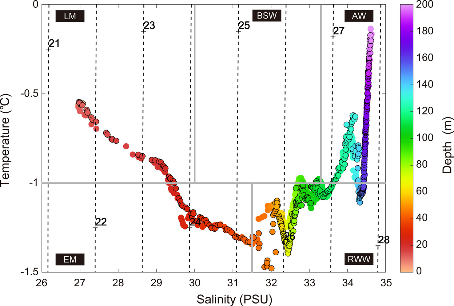
Figure 6 Temperature-salinity plot of CTD data collected during daytime and nighttime (black-edged circles). The colors of the dots indicate water depth. Density contours, represented by the black dashed lines, were overlaid on the T/S diagram. Major water masses in the study area are delineated by thick gray lines. The water masses are as follows: LM, late season meltwater; EM, early season meltwater; RWW, remnant winter water; BSW, Bering summer water; and AW, Atlantic water.

Zooplankton community

All net results showed that copepods, in both adult and copepodite stages, accounted for more than > 79% of the total zooplankton abundance (Table 2). The key copepod species composition, expressed as a percentage hereafter, is the result of the adult and copepodite stages combined (Figure 7). At night, the zooplankton community was dominated by C. glacialis (74.8%) between the surface and 25 m depth, while M. longa, C. glacialis, and C. hyperboreus contributed 38.4, 31.5, and 22.2% of the zooplankton abundance from the surface to 55 m, respectively. M. longa and C. hyperboreus were distributed at a relatively deeper depth than C. glacialis at night. In the daytime, the zooplankton community was dominated by C. glacialis (81.6%) between the surface and 25 m depth, whereas C. glacialis and C. hyperboreus accounted for 42.2 and 36.5% of the zooplankton abundance between the surface and 55 m depth, respectively. In contrast to nighttime observations, M. longa was not observed between the surface and 55 m during the daytime, and M. longa contributed 49.4% of the zooplankton abundance between the surface and 135 m depth.

TABLE 2

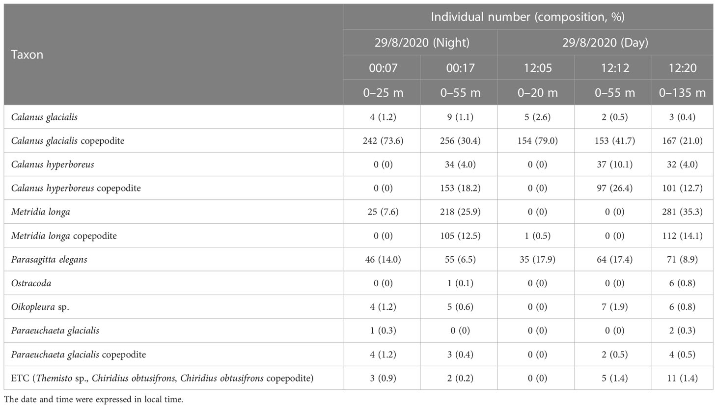
Table 2 Summary of the abundance (ind. m^-3) and composition (%) of zooplankton in each bongo net sample.

FIGURE 7

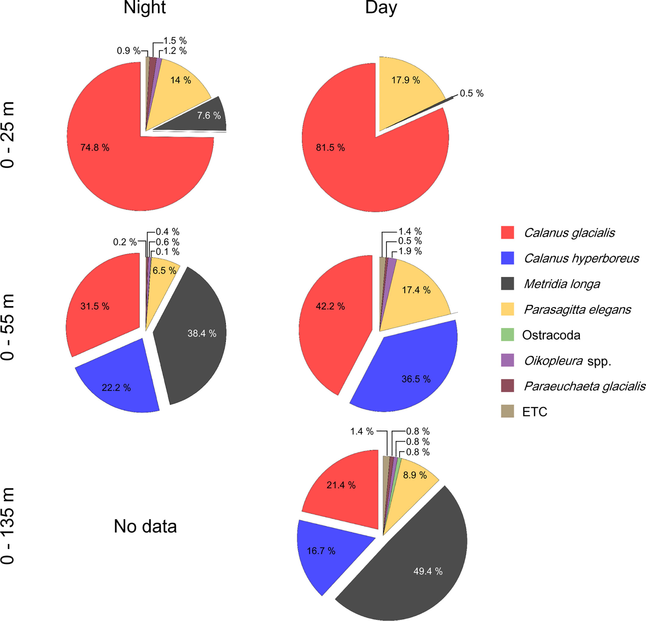
Figure 7 Pie chart of the zooplankton community composition of abundance from Table 2. The composition of copepod species (C. glacialis, C. hyperboreus, M. longa, P. glacialis, C. obtusifrons) was combined with adult and copepodite stages. The ETC categories include Themisto sp., C. obtusifrons.

The vertical distributions of the dominant copepod species were identified by calculating the abundance differences for the same species at different depths and confirming whether they were collected or not (Table 2; Figure 7). C. glacialis and C. hyperboreus were predominantly found above 25 m and between 25 and 55 m in the water column during the day and night, respectively, even though they were also collected at depths from 0–55 m and 0–135 m. The abundance differences for these species among depths were confirmed to be less than 1%. M. longa was mainly observed between 25 and 55 m water column at night, with an abundance approximately 13% higher above 55 m than above 25 m. During the day, M. longa was primarily collected above 135 m than 55 m. These results indicate that C. glacialis and C. hyperboreus did not perform DVM, while M. longa conducted DVM.

The key copepod species listed above were followed by Parasagitta elegans, which composed approximately 7–18% of the community composition (Table 2; Figure 7). The number of collected P. elegans did not increase in proportion to the net depth, and the numbers of P. elegans collected from the 25-m depth during the daytime and nighttime exhibited differences of only 36 individuals compared to the results collected at other depths. From this, we thought that P. elegans was mainly distributed above 25 m during the day and at night.

Length-frequency distributions of the key copepod species

The prosome lengths of C. glacialis, C. hyperboreus, and M. longa individuals were measured to identify the acoustic backscatter among the three copepod species (Figure 8). The length-frequency distribution of C. glacialis (n=150) measured from five net surveys ranged between 2.14 and 5.41 mm, with a mean length of 3.43 mm (standard deviation (S.D.) = 0.61). The measured length-frequency distribution of C. hyperboreus (n = 90) ranged from 3.80 to 7.77 mm, with a mean length of 5.94 mm (S.D. = 0.94). The measured length-frequency distribution (n=90) of M. longa ranged from 2.03 to 3.92 mm, and its mean length was 2.94 mm (S.D. = 0.34).

FIGURE 8

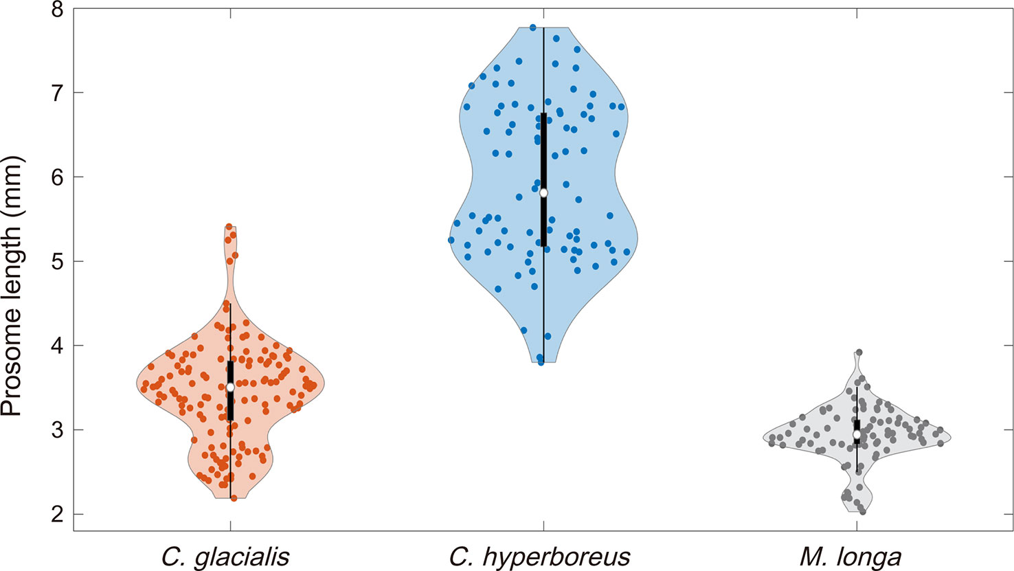
Figure 8 Length-frequency distributions of C. glacialis, C. hyperboreus, and M. longa. A violin plot is a combination of a box plot and a kernel density plot. The red, blue, and dark gray dots represent the prosome lengths of C. glacialis, C. hyperboreus, and M. longa, respectively. Each white circle within each boxplot indicates the median value.

Vertical distribution of the key copepod species

Calanus glacialis, C. hyperboreus, and M. longa show different vertical behaviors. The SSLs of C. glacialis and C. hyperboreus were continuously observed in daytime and nighttime in the water column above 20 m and between 30 and 55 m, respectively. On the other hand, DVM behaviors were clearly observed in accordance with the light differences between daytime and nighttime in the SSL of M. longa between 30 and 135 m. The acoustic backscatter of C. glacialis was distributed with a thickness of approximately 4–8 m at depths of 15−25 m, and the mean Sv was -71.3 dB (S.D. = 1.2) (Figure 9A). The acoustic backscatter of C. hyperboreus was distributed at depths of 30−57 m with a thickness of approximately 5 to 20 m, and the mean Sv was -72.9 dB (S.D. = 0.8) (Figure 9B). The mean Sv of the acoustic backscatter of M. longa was -79.6 dB (SD = 0.4); in the daytime, this acoustic backscatter was distributed with a 25- to 33-m thickness between the depths of 25 to 62 m, and at night, it was distributed with a thickness of approximately 15–45 m at depths of 88–134 m (Figure 9C). The diel velocity of M. longa was calculated using the start and end times of the ascending and descending components of the two cycles. In the first cycle, the ascending and descending rates of M. longa were 0.79 and 1.26 (cm s^-1), respectively, and in the second period were 1.26 and 1.11 (cm s^-1), respectively.

FIGURE 9

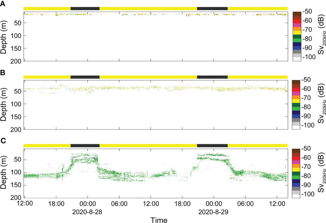
Figure 9 The classification results of the acoustic backscatters of three copepod species: the acoustic backscatter of (A) C. glacialis, (B) C. hyperboreus, and (C) M. longa separated by the depth limitation conditions derived in step III in Figure 3H.

Environmental factors influencing the vertical distribution

To understand the marine environmental characteristics of the water column in which C. glacialis, C. hyperboreus, and M. longa are distributed, the vertical profiles of the water temperature, salinity, and fluorescence were presented alongside the acoustic backscatter distributions of the three copepod species (Figure 10). The C. glacialis observed at depths of 15–25 m were distributed in the water temperature range between -1.16 and -0.56 °C, the salinity range between 26.97–29.64 PSU and in an environment with a low phytoplankton biomass (Figures 10A–C). Calanus hyperboreus was observed at depths of 25–55 m, where the water temperature ranged from -1.34 to -1.12°C, the salinity ranged from 29.63 to 32.22 PSU, and the environment had a high phytoplankton biomass (Figures 10D, E). M. longa individuals observed at depths of 25–135 m were distributed in the water temperature range between -1.34 and -0.72 °C, and the salinity range between 29.64 and 34.25 PSU in an environment displaying large phytoplankton biomass fluctuations (Figures 10G–I). Compared to C. glacialis, C. hyperboreus was distributed in an environment with relatively cold water temperatures, high salinity, and a large phytoplankton biomass. M. longa is distributed in an environment with relatively large water temperature and salinity fluctuations compared to the two Calanus species. DVM behavior enables zooplankton to encounter varying environmental conditions (Häfker et al., 2022). In the case of M. longa, DVM resulted in a distinct distribution pattern across different environments during the day and at night. Specifically, this species inhabits a cold (-1.47 – -1.1 °C) and low salinity (29.65–32.46 PSU) environment with high phytoplankton biomass (0.13–3.94 µg L^-1) during the night, while it preferred a warm (-1.09 – -0.72 °C) and high salinity (33.05–34.21 PSU) with low phytoplankton biomass (0.09–0.13 µg L^-1) during the day (Figures 5D; 11).

FIGURE 10

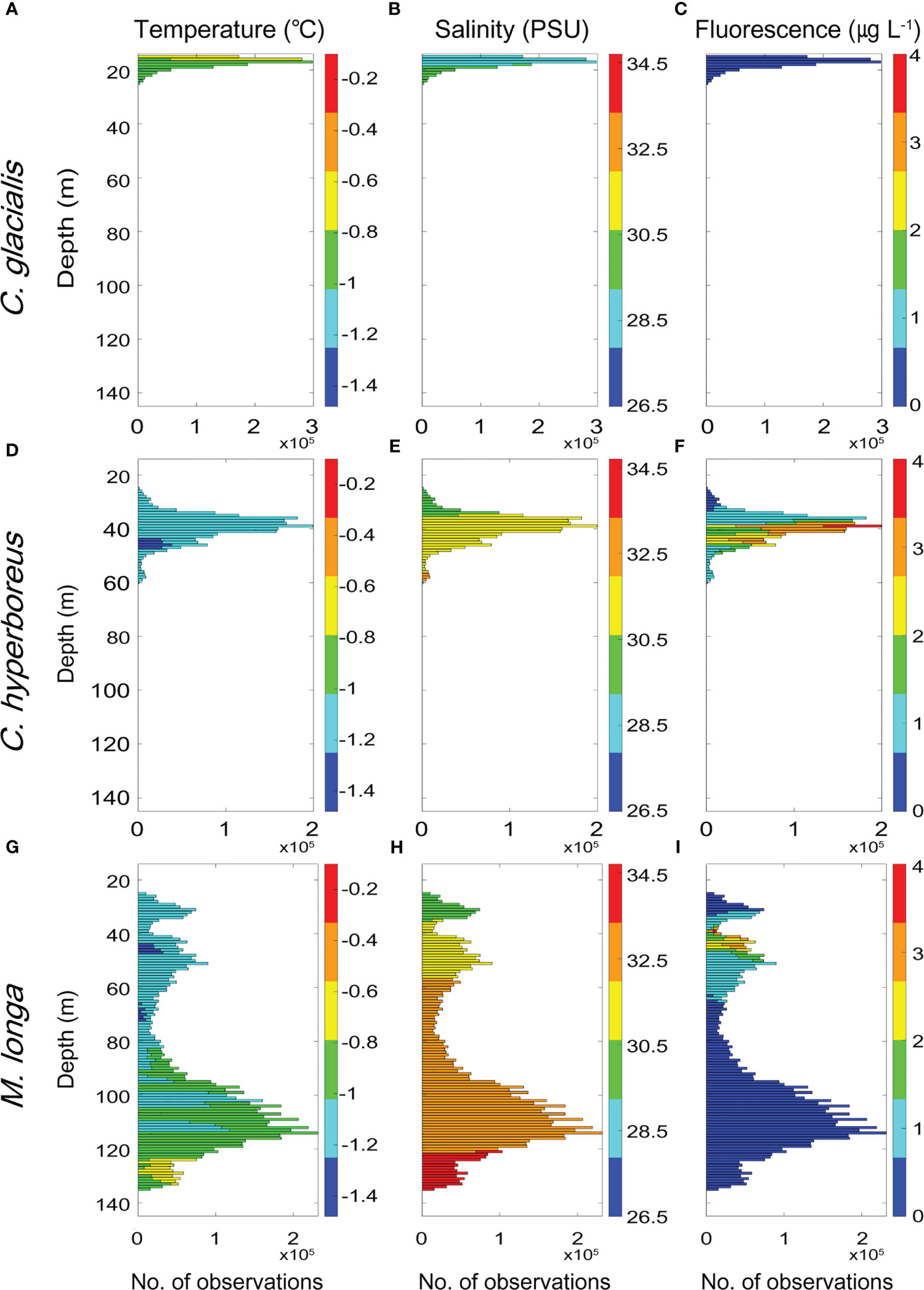
Figure 10 Frequency distributions of the C. glacialis (A–C), C. hyperboreus (D–F) and M. longa (G–I) observations (excluding 0 values) as a function of water temperature (°C), salinity (PSU) and fluorescence (µg L^-1).

FIGURE 11

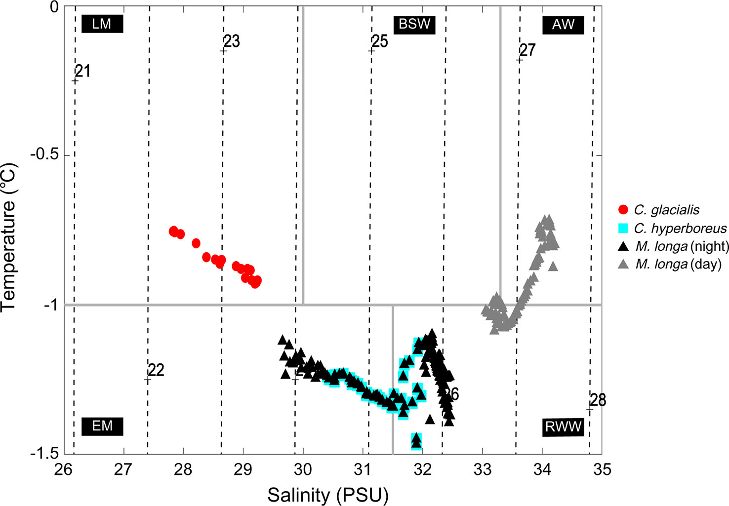
Figure 11 The vertical distribution of the key copepod species in the classified water masses. Red dots and cyan squares represent the vertical distributions of C. glacialis and C. hyperboreus, respectively. The black and gray triangles denote the vertical distribution of M. longa at nighttime and daytime, respectively. The characterization of the water masses follows Gong and Pickart (2015) and Linders et al. (2017). The water masses are as follows: LM, late season meltwater; EM, early season meltwater; RWW, remnant winter water; BSW, Bering summer water; and AW, Atlantic water. Acoustic backscatters attributed to three species were extracted and analyzed within 1 hour before and after the first net survey time conducted during the daytime or nighttime.

The vertical distribution of each key copepod species and its relationship to the marine environments were analyzed using the Pearson correlation test. At night, the vertical distribution of C. glacialis was correlated with temperature (r = 0.97, p < 0.01) and salinity (r = -0.94, p < 0.01), that of C. hyperboreus was only correlated with fluorescence (r = 0.61, p < 0.01), and that of M. longa was correlated with temperature (r = -0.61, p < 0.01) and fluorescence (r = 0.48, p < 0.01). During the day, the vertical distribution of C. glacialis was correlated with temperature (r = 0.83, p < 0.01) and salinity (r = -0.84, p < 0.01), that of C. hyperboreus was correlated with fluorescence (r = 0.57, p < 0.01) and that of M. longa was correlated with temperature (r = 0.72, p < 0.01) and salinity (r = 0.82, p < 0.01). At the same time, during the day and night, C. glacialis presented a strong positive correlation with temperature and a negative correlation with salinity, and C. hyperboreus showed a strong positive correlation with fluorescence.

The acoustic backscatters identified for C. glacialis, C. hyperboreus, and M. longa showed clear vertical distribution differences (Figure 11). Calanus glacialis was distributed in the late season meltwater in both daytime and nighttime. Calanus hyperboreus was also distributed in the early season meltwater and remnant winter water regardless of the time of day/night, and the distribution ratios in these two water masses were 65.2% and 34.8%, respectively. M. longa was distributed in the early season meltwater and remnant winter water at night, as in the case of C. hyperboreus, and the distribution percentages for each water mass were 34.9% and 65.1%, respectively. This species was distributed in the remnant winter water, Bering summer water and Atlantic water during the daytime at distribution rates of 42.0%, 8.6% and 49.4%, respectively.

Discussion

Uncertainties in acoustic identification

While the net data contained counts of individuals of all ages and stages, only those above detectable length were included in the acoustic data. This might cause some uncertainties when interpreting the vertical distribution of the dominant species based on acoustically identified results. Our net results revealed that C. glacialis, C. hyperboreus, and M. longa were the dominant species. Based on this, the length distributions of three key copepods above 2 mm were used for acoustic identification due to the detectable minimum length at 200 kHz. Because the composition of the dominant species will not change even when counting individuals above 2 mm, it was considered that our acoustic results accurately reflected the vertical distribution of the dominant species identified by the nets.

P. elegans presented the dominant component (7–18% of the total community), followed by three key copepod species (Table 2). Coexisting with these key copepod species, the acoustic backscatter of P. elegans may influence their acoustic identification. P. elegans specimens collected at depths above 25 m during day and night showed only slight differences of up to 36 individuals compared to those collected in deeper water. This suggests that P. elegans was not evenly distributed throughout the entire water column but rather mainly distributed in a limited water column (< 25 m) where C. glacialis was also present. The mean length of the P. elegans in our study was 17.17 mm (S.D. = 2.97, n = 150), characterizing the stages between Cohort0 and Cohort1 (Grigor et al., 2014). In these stages, one individual Calanus spp. exhibits the same Sv as that of at least five P. elegans (Chaetognatha) individuals (Mair et al., 2005; Berge et al., 2014). The population ratio of P. elegans to C. glacialis found in our study was less than 1, indicating that the acoustic backscatter of P. elegans is considerably weaker than that of C. glacialis. Therefore, we concluded that the acoustic identification of C. glacialis was not significantly affected by the acoustic backscatter of P. elegans.

Acoustic identification of C. glacialis, C. hyperboreus, and M. longa

The Sv_{200-120 kHz} ranges required to identify acoustic backscatters of the key copepod species were determined from the length-frequency distributions of each species. However, using only the length-frequency distribution makes it difficult to identify acoustic backscatter if different copepod species have similar length ranges. Therefore, to ensure the effective identification of the acoustic backscatter of the key copepods, we considered not only the length-frequency distribution of the three species but also the differences in their vertical distributions. This method resulted in three clearly distinguished acoustic backscatter signatures compared to those obtained under the existing method in which only the length-frequency distributions are used (Figure 3H).

While the net sampling (Table 2) showed that C. glacialis was distributed within water depths above 25 m, the acoustic backscatter of this species was mainly distributed at depths of 15–20 m and 30–55 m (top in Figure 3H). Because the net survey results indicated that C. glacialis was distributed above a depth of 25 m, the acoustic backscatter identified at depths of 30–55 m can be considered to be that of another organism with a length range similar to that of this species. Our net sampling results revealed that C. hyperboreus was predominantly distributed at depths between 25 and 55 m. The measured length distribution range of C. hyperboreus between 3.80 and 5.41 mm overlapped with the measured length range of C. glacialis (Figure 8). Therefore, we considered that the acoustic backscatter identified for C. glacialis at 30–55-m depths was that of C. hyperboreus, and this acoustic backscatter was thus excluded from the acoustic identification of C. glacialis. In the case of C. hyperboreus, the net survey indicated that this species was distributed in the depth range of 25 to 55 m (Table 2), whereas the acoustic backscatters were mainly distributed at depths of 15–25 m and 30–55 m (middle in Figure 3H). This finding suggested that the acoustic backscatter identified as C. hyperboreus at depths of 15–25 m was that of a different organism. The main species collected with the nets above the 25-m depth was C. glacialis (Table 2), which had the same length ranges as C. hyperboreus in the range of 3.80–5.41 mm. Therefore, the acoustic backscatter identified as those of C. hyperboreus at 15–25-m depths was excluded, as these acoustic backscatters were considered to be sourced from C. glacialis, which had a similar length range as C. hyperboreus. M. longa was distributed at depths of 55–135 m during the daytime and above 55 m at night according to the net survey (Table 2). However, acoustic backscatters of this species were found not only at depths ranging from 100–135 m and 25–55 m during the daytime and at nighttime, respectively, but were also found to be continuously distributed above a depth of 55 m regardless of the time of day (lower in Figure 3H). Based on the net results, the acoustic backscatter consistently observed above 55 m was thus inferred to be that of a different organism. In the net survey, C. glacialis and C. hyperboreus were found to be distributed at depths above 25 m and ranging from 30–55 m, respectively (Table 2); in addition, the length ranges of these species overlapped with that of M. longa in the ranges of 2.14–3.92 mm and 3.80–3.92 mm, respectively. Moreover, because we extracted only the late juveniles (CIV–CVI) and adult specimens in this study when measuring the length distributions of copepods, the possibility that the length distribution of C. hyperboreus before CIV may overlap with the length distribution of M. longa over a wider range was present. Madsen et al. (2001) reported that when studying the length distributions of Calanus species during the copepodite stages in the Arctic Ocean, the pre-CIV stage of C. hyperboreus exhibited a length distribution of < 3.9 mm. From this finding, it may be deduced that the acoustic backscatters observed at depths above 25 m and from 30–55 m during the day can be attributed to C. glacialis and C. hyperboreus, which have length distributions similar to that of M. longa; therefore, these acoustic backscatters were excluded when identifying the acoustic backscatter of M. longa.

The results obtained when identifying the acoustic backscatter of the three copepod species by considering both their length-frequency distribution and the vertical distributions showed that the vertical distribution differences among the three species confirmed by the net surveys can be critical for classifying among their acoustic backscatters. Understanding the exact vertical distribution of the organism of interest is important because this information can subsequently be used to identify the acoustic backscatter of not only copepods but also other marine organisms.

Vertical distribution of Arctic copepods

In this study, C. glacialis was found to be distributed in the late season meltwater and did not exhibit DVM behaviors. The observed vertical distribution of C. glacialis appeared to be related to its feeding activities. The late season meltwater, which forms by the melting of sea ice, is an environment in which the surface layer is stabilized by the density difference (Gong and Pickart, 2015; Pacini et al., 2019), where phytoplankton and microzooplankton, the food sources of C. glacialis, can thoroughly aggregate (Campbell et al., 2009; Leu et al., 2015). The omnivorous C. glacialis prefers to feed on microzooplankton in environments with low phytoplankton biomasses (Levinsen et al., 2000; Campbell et al., 2009). Microzooplankton prefer picophytoplankton as their food (Yang et al., 2015), and their biomass increases rapidly when phytoplankton flourish (Campbell et al., 2009). The pelagic phytoplankton bloom identified in this study area thrives between June and July (Arrigo and Van Dijken, 2011), and the survey performed in this study was conducted after these pelagic phytoplankton flourished. The water column in which C. glacialis was distributed had a low phytoplankton biomass and a large picophytoplankton contribution (Figure 5D). From this, we deduced that the microzooplankton biomass was high in the late season meltwater. Calanus spp. individuals who do not have sufficient energy to enter overwintering remain in the upper water layer until late summer or autumn to feed (Søreide et al., 2010; Rabindranath et al., 2011). Because the observed C. glacialis were collected within the upper 25 m of water, it is highly likely that they were feeding for energy storage. They may have exhibited non-DVM behaviors because it is more important to store energy through feeding irrespective of the time of day or night than to undergo DVM. The absence of DVM behavior of C. glacialis may be attributed to a low predation pressure environment. Predator avoidance has been proposed as one of the key factors influencing zooplankton DVM behavior (Lampert, 1989; Bollens and Frost, 1991; Hays, 1995; Daase et al., 2016). Potential predators of copepods in our study area include Arctic cod (Boreogadus saida), amphipod (Themisto sp.), and chaetognaths (Parasagitta elegans) (Fortier et al., 2001; Pinchuk and Eisner, 2017; Grigor et al., 2020). Juvenile Arctic cod, as a visual predator, is mainly distributed in water temperatures between 1 and 6°C (Vestfals et al., 2019; Maznikova et al., 2023). However, the water temperature environment in our study region was less than 0 °C (Figure 5A), indicating a significant difference from the typical temperature range where they are known to be abundant. Another visual predator, Themisto sp. was rarely collected in the nets, while P. elegans, a tactile predator, was the most abundant animal collected in nets, followed by three key copepod species (Table 2). In this study, the mean length of P. elegans was 17.17 mm (S.D. = 2.97, n = 150), ranging from 10.58 to 23.76 mm. Based on size classes, P. elegans in the 10-20 mm range exhibited a preference for smaller copepods (1.0–3.5 mm) as prey compared to C. glacialis (Patuła et al., 2023). Our findings indicate that the distribution of C. glacialis was influenced by a low predation pressure environment. Thus, we concluded that the distribution of C. glacialis without DVM behavior in the late season meltwater could be related to their feeding activity and a lower predation pressure environment. Additional research in which the food sources of C. glacialis are analyzed is needed to confirm this result and to understand the spatial distributions of microzooplankton.

Our study found that C. hyperboreus was distributed in the early season meltwater and upper remnant winter water, and no DVM behaviors were observed. The observed vertical distribution of C. hyperboreus appeared to be related to its feeding activity. C. hyperboreus is a representative herbivorous copepod that mainly feeds on large phytoplankton, such as diatoms (Ashjian et al., 2003; Choi et al., 2021; Daase et al., 2021). In the Siberian Sea and Chukchi Sea, adjacent to the survey area, chl-a has been observed in large amounts in the water column at depths of approximately 30–55 m (Arrigo and Van Dijken, 2011; Choi et al., 2021; Jung et al., 2021; Kim et al., 2021); this depth is consistent with the observed vertical distribution of phytoplankton. The ratio of large-sized micro phytoplankton was found to be high in the water layers in which C. hyperboreus was distributed. The C. hyperboreus individuals collected in the upper water column were likely to be entities that require energy storage to enter the dormant phase. In addition, the observed low predation pressure environment for C. glacialis might have similarly influenced the distribution and behavior of C. hyperboreus. The results suggest that C. hyperboreus was able to efficiently feed without DVM in the early season meltwater and upper remnant winter water, which were rich in phytoplankton and characterized by low predation pressure.

M. longa showed a distinct DVM consistent with solar cycles. M. longa individuals were located in the upper water column, where C. hyperboreus was also distributed at night, while M. longa was distributed at depths between approximately 100 and 135 m during the day. Such a diel vertical distribution appeared to be related to light intensity changes, the life strategy of the species, the distribution of their potential food, and the seawater density. Previous studies (Falkenhaug et al., 1997; Fortier et al., 2001; Ashjian et al., 2003; Daase et al., 2008) have reported DVM behaviors of M. longa consistent with the solar cycle; these findings are consistent with the results of our study. The changes in solar radiation can be regarded as a signal that informs the timing of the vertical movement of copepods (La et al., 2018). Fortier et al. (2001) observed that M. longa exhibited DVM behavior in a sea ice-covered environment in response to low irradiance variations (0.07–0.21%) from the atmosphere to the water. The observations in this study indicated that the variation in solar radiation could be the cause of the DVM of M. longa. M. longa, which lacks seasonal vertical migration, is less sensitive to phytoplankton production than Calanus spp. (Ashjian et al., 2003). Therefore, M. longa shows a relatively flexible vertical distribution compared to Calanus species (Ashjian et al., 2003; Daase et al., 2008) and feeds on phytoplankton in spring and summer and on zooplankton in winter (Ashjian et al., 2003). The vertical distribution of M. longa observed in this study was wide compared to that of Calanus spp. and was distributed in the water column, in which the phytoplankton biomass was high at night. This result is consistent with the findings of previous studies (Ashjian et al., 2003; Daase et al., 2008). The density gradient differences within a water layer can act as a physical barrier to the vertical migration of copepods (Woodson et al., 2007; Berge et al., 2014; La et al., 2018). The upper and lower boundary depths of the M. longa DVM observed in this study were 25 m and 135 m, respectively (Figure 9C), and the peak values of the absolute density gradient were observed at depths of 18 m and 134 m, respectively, near these two boundaries (Figure 5C). These results indicate that the depth range of the observed DVM of M. longa can be determined by the density gradient. The differences in observed vertical behavior between the two Calanus species and M. longa are linked to their morphological differences, resulting in contrasting swimming abilities (Hays et al., 1997; Torgersen, 2001). The swimming speed of M. longa is approximately 10 times faster than that of Calanus spp., so it can be better detected by visual and nonvisual predators (Torgersen, 2001). Because of this, M. longa may have more adapted DVM, such as predator-avoiding behavior, than Calanus spp. (Daase et al., 2008).

Conclusions

In this study, we provide information on the DVM behavior in C. glacialis, C. hyperboreus, and M. longa and their different vertical distributions in the ESCM region following the midnight sun period. In addition, marine environmental factors affecting the vertical distributions of key copepod species were investigated. Our results identified the acoustic backscatters of key copepod species for the first time and made it possible to estimate their vertical distributions and migrations at high resolution that were roughly identified by only net collection (Daase et al., 2008). Neither Calanus species exhibited DVM behavior regardless of the diel light cycle and was distributed in the upper water column. On the other hand, M. longa showed a DVM consistent with the diel light cycles and exhibited a wider vertical distribution than those of the two Calanus species. The vertical distribution ranges of C. glacialis and M. longa were controlled by the density gradient of the water column, while the water temperature and phytoplankton biomass influenced the vertical distribution range of C. hyperboreus. The western Arctic Ocean is undergoing rapid changes in its hydrological properties and overall circulation due to increased AW inflows (Polyakov et al., 2017; Ardyna and Arrigo, 2020). For example, Jung et al. (2021) reported that with the invasion of Atlantic-origin cold saline water into the western Arctic Ocean, not only did phytoplankton blooms in oligotrophic surface waters and the SCM layer become shallow but also the density gradient of the water column also fluctuated. This may lead to the vertical distribution of C. glacialis and C. hyperboreus being shallower and may shorten the vertical migration range of M. longa. Our results highlight that high-resolution observation of the vertical distribution of key copepod species is essential to understanding how key copepods adapt to the rapidly changing Arctic Ocean environment.

Data availability statement

The original contributions presented in the study are included in the article/Supplementary Materials. Further inquiries can be directed to the corresponding author.

Author contributions

WS collected and analyzed the acoustic, zooplankton, and marine environmental data and wrote the manuscript. HL designed the study and carried out supervision and validation. J-HK analyzed the zooplankton community composition, and EY supported chlorophyll data and research funding. All authors contributed to the article and approved the submitted version.

Funding

This research was supported by Korea Institute of Marine Science & Technology Promotion (KIMST) funded by the Ministry of Oceans and Fisheries (20210605, Korea-Arctic Ocean Warming and Response of Ecosystem, KOPRI).

Acknowledgments

We acknowledge the support and dedication of the captain and crew of IBRV ARAON for completing the field work with positive energy. We would like to thank Dr. Euna Yoon for providing valuable advice on the analysis of the DWBA model. We would also like to thank Jae il Yoo for providing valuable advice on the analysis of PAR data. Finally, we would like to thank the reviewers for providing valuable advice, counsel, and guidance.

Conflict of interest

The authors declare that the research was conducted in the absence of any commercial or financial relationships that could be construed as a potential conflict of interest.

Publisher’s note

All claims expressed in this article are solely those of the authors and do not necessarily represent those of their affiliated organizations, or those of the publisher, the editors and the reviewers. Any product that may be evaluated in this article, or claim that may be made by its manufacturer, is not guaranteed or endorsed by the publisher.

References

Ardyna M., Arrigo K. R. (2020). Phytoplankton dynamics in a changing Arctic ocean. Nat. Clim. Change 10, 892–903. doi: 10.1038/s41558-020-0905-y

CrossRef Full Text | Google Scholar

Arrigo K. R., Van Dijken G. L. (2011). Secular trends in Arctic ocean net primary production. J. Geophys. Res. Ocean. 116, 1–15. doi: 10.1029/2011JC007151

CrossRef Full Text | Google Scholar

Ashjian C. J., Campbell R. G., Welch H. E., Butler M., Van Keuren D. (2003). Annual cycle in abundance, distribution, and size in relation to hydrography of important copepod species in the western Arctic ocean. Deep. Res. Part I Oceanogr. Res. Pap. 50, 1235–1261. doi: 10.1016/S0967-0637(03)00129-8

CrossRef Full Text | Google Scholar

Benfield M. C., Davis C. S., Gallager S. M. (2000). Estimating the in-situ orientation of calanus finmarchicus on georges bank using the video plankton recorder. Plankt. Biol. Ecol. 47, 69–72.

Google Scholar

Benoit D., Simard Y., Gagné J., Geoffroy M., Fortier L. (2010). From polar night to midnight sun: photoperiod, seal predation, and the diel vertical migrations of polar cod (Boreogadus saida) under land fast ice in the Arctic ocean. Polar Biol. 33, 1505–1520. doi: 10.1007/s00300-010-0840-x

CrossRef Full Text | Google Scholar

Berge J., Cottier F., Varpe Ø., Renaud P. E., Falk-Petersen S., Kwasniewski S., et al. (2014). Arctic Complexity: a case study on diel vertical migration of zooplankton. J. Plankton Res. 36, 1279–1297. doi: 10.1093/plankt/fbu059

PubMed Abstract | CrossRef Full Text | Google Scholar

Blachowiak-Samolyk K., Kwasniewski S., Richardson K., Dmoch K., Hansen E., Hop H., et al. (2006). Arctic Zooplankton do not perform diel vertical migration (DVM) during periods of midnight sun. Mar. Ecol. Prog. Ser. 308, 101–116. doi: 10.3354/meps308101

CrossRef Full Text | Google Scholar

Blachowiak-Samolyk K., Søreide J. E., Kwasniewski S., Sundfjord A., Hop H., Falk-Petersen S., et al. (2008). Hydrodynamic control of mesozooplankton abundance and biomass in northern Svalbard waters (79-81°N). Deep. Res. Part II Top. Stud. Oceanogr. 55, 2210–2224. doi: 10.1016/j.dsr2.2008.05.018

CrossRef Full Text | Google Scholar

Bollens S. M., Frost B. W. (1991). Diel vertical migration in zooplankton: rapid individual response to predators. J. Plankton Res. 13, 1359–1365. doi: 10.1093/plankt/13.6.1359

CrossRef Full Text | Google Scholar

Brierley A. S. (2014). Diel vertical migration. Curr. Biol. 24, R1074–R1076. doi: 10.1016/j.cub.2014.08.054

PubMed Abstract | CrossRef Full Text | Google Scholar

Brierley A. S., Ward P., Watkins J. L., Goss C. (1998). Acoustic discrimination of southern ocean zooplankton. Deep. Res. Part II Top. Stud. Oceanogr. 45, 1155–1173. doi: 10.1016/S0967-0645(98)00025-3

CrossRef Full Text | Google Scholar

Campbell R. G., Sherr E. B., Ashjian C. J., Plourde S., Sherr B. F., Hill V., et al. (2009). Mesozooplankton prey preference and grazing impact in the western Arctic ocean. Deep. Res. Part II Top. Stud. Oceanogr. 56, 1274–1289. doi: 10.1016/j.dsr2.2008.10.027

CrossRef Full Text | Google Scholar

Choi H., Won H., Kim J. H., Yang E. J., Cho K. H., Lee Y., et al. (2021). Trophic dynamics of calanus hyperboreus in the pacific Arctic ocean. J. Geophys. Res. Ocean. 126, 1–15. doi: 10.1029/2020JC017063

CrossRef Full Text | Google Scholar

Cottier F. R., Tarling G. A., Wold A., Falk-Petersen S. (2006). Unsynchronized and synchronized vertical migration of zooplankton in a high arctic fjord. Limnol. Oceanogr. 51, 2586–2599. doi: 10.4319/lo.2006.51.6.2586

CrossRef Full Text | Google Scholar

Daase M., Berge J., Søreide J. E., Falk-Petersen S. (2021). Ecology of Arctic pelagic communities. in Arctic Ecology. Thomas D. N., ed., Wiley. pp. 219–259. doi: 10.1002/9781118846582.ch9

CrossRef Full Text | Google Scholar

Daase M., Eiane K. (2007). Mesozooplankton distribution in northern Svalbard waters in relation to hydrography. Polar Biol. 30, 969–981. doi: 10.1007/s00300-007-0255-5

CrossRef Full Text | Google Scholar

Daase M., Eiane K., Aksnes D. L., Vogedes D. (2008). Vertical distribution of calanus spp. and metridia longa at four Arctic locations. Mar. Biol. Res. 4, 193–207. doi: 10.1080/17451000801907948

CrossRef Full Text | Google Scholar

Daase M., Hop H., Falk-Petersen S. (2016). Small-scale diel vertical migration of zooplankton in the high Arctic. Polar Biol. 39, 1213–1223. doi: 10.1007/s00300-015-1840-7

CrossRef Full Text | Google Scholar

Darnis G., Barber D. G., Fortier L. (2008). Sea Ice and the onshore-offshore gradient in pre-winter zooplankton assemblages in southeastern Beaufort Sea. J. Mar. Syst. 74, 994–1011. doi: 10.1016/j.jmarsys.2007.09.003

CrossRef Full Text | Google Scholar

Demer D. A., Conti S. G. (2005). New target-strength model indicates more krill in the southern ocean. ICES J. Mar. Sci. 62, 25–32. doi: 10.1016/j.icesjms.2004.07.027

CrossRef Full Text | Google Scholar

De Robertis A., Higginbottom I. (2007). A post-processing technique to estimate the signal-to-noise ratio and remove echosounder background noise. ICES J. Mar. Sci. 64, 1282–1291. doi: 10.1093/icesjms/fsm112

CrossRef Full Text | Google Scholar

Emery W. J., Thomson R. E. (2001). Data analysis methods in physical oceanography. (Elsevier Science BV: Amsterdam, The Netherlands), 83–94.

Google Scholar

Falkenhaug T., Tande K. S., Semenova T. (1997). Diel, seasonal and ontogenetic variations in the vertical distributions of four marine copepods. Mar. Ecol. Prog. Ser. 149, 105–119. doi: 10.3354/meps149105

CrossRef Full Text | Google Scholar

Falk-Petersen S., Leu E., Berge J., Kwasniewski S., Nygård H., Røstad A., et al. (2008). Vertical migration in high Arctic waters during autumn 2004. Deep. Res. Part II Top. Stud. Oceanogr. 55, 2275–2284. doi: 10.1016/j.dsr2.2008.05.010

CrossRef Full Text | Google Scholar

Feng Z., Ji R., Ashjian C., Campbell R., Zhang J. (2018). Biogeographic responses of the copepod calanus glacialis to a changing Arctic marine environment. Glob. Change Biol. 24, e159–e170. doi: 10.1111/gcb.13890

CrossRef Full Text | Google Scholar

Forest A., Tremblay J., Éric, Gratton Y., Martin J., Gagnon J., Darnis G., et al. (2011). Biogenic carbon flows through the planktonic food web of the amundsen gulf (Arctic ocean): a synthesis of field measurements and inverse modeling analyses. Prog. Oceanogr. 91, 410–436. doi: 10.1016/j.pocean.2011.05.002

CrossRef Full Text | Google Scholar

Fortier M., Fortier L., Hattori H., Saito H., Legendre L. (2001). Visual predators and the diel vertical migration of copepods under Arctic sea ice during the midnight sun. J. Plankton Res. 23, 1263–1278. doi: 10.1093/plankt/23.11.1263

CrossRef Full Text | Google Scholar

Gastauer S., Nickels C. F., Ohman M. D. (2022). Body size- and season-dependent diel vertical migration of mesozooplankton resolved acoustically in the San Diego trough. Limnol. Oceanogr. 67, 300–313. doi: 10.1002/lno.11993

CrossRef Full Text | Google Scholar

Gong D., Pickart R. S. (2015). Summertime circulation in the eastern chukchi Sea. Deep. Res. Part II Top. Stud. Oceanogr. 118, 18–31. doi: 10.1016/j.dsr2.2015.02.006

CrossRef Full Text | Google Scholar

Grigor J. J., Schmid M. S., Caouette M., St.-Onge V., Brown T. A., Barthélémy R. M. (2020). Non-carnivorous feeding in Arctic chaetognaths. Prog. Oceanogr. 186, 102388. doi: 10.1038/s42003-022-03472-z

CrossRef Full Text | Google Scholar

Grigor J. J., Søreide J. E., Varpe Ø. (2014). Seasonal ecology and life-history strategy of the high-latitude predatory zooplankter parasagitta elegans. Mar. Ecol. Prog. Ser. 499, 77–88. doi: 10.3354/meps10676

CrossRef Full Text | Google Scholar

Häfker N. S., Connan-McGinty S., Hobbs L., McKee D., Cohen J. H., Last K. S. (2022). Animal behavior is central in shaping the realized diel light niche. Commun. Biol. 5, 1–8. doi: 10.1038/s42003-022-03472-z

PubMed Abstract | CrossRef Full Text | Google Scholar

Hays G. C. (1995). Ontogenetic and seasonal variation in the diel vertical migration of the copepods metridia lucens and metridia longa. Limnol. Oceanogr. 40, 1461–1465.

Google Scholar

Hays G. C., Warner A. J., Tranter P. (1997). Why do the two most abundant copepods in the north Atlantic differ so markedly in their diel vertical migration behaviour? J. Sea Res. 38, 85–92. doi: 10.1016/S1385-1101(97)00030-0

CrossRef Full Text | Google Scholar

Hop H., Gjøsæter H. (2013). Polar cod (Boreogadus saida) and capelin (Mallotus villosus) as key species in marine food webs of the Arctic and the Barents Sea. Mar. Biol. Res. 9, 878–894. doi: 10.1080/17451000.2013.775458

CrossRef Full Text | Google Scholar

Jarolím O., Kubečka J., Čech M., Vašek M., Peterka J., Matěna J. (2010). Sinusoidal swimming in fishes: the role of season, density of large zooplankton, fish length, time of the day, weather condition and solar radiation. Hydrobiologia 654, 253–265. doi: 10.1007/s10750-010-0398-1

CrossRef Full Text | Google Scholar

Jung J., Cho K. H., Park T., Yoshizawa E., Lee Y., Yang E. J., et al. (2021). Atlantic-Origin cold saline water intrusion and shoaling of the nutricline in the pacific Arctic. Geophys. Res. Lett. 48, 1–10. doi: 10.1029/2020GL090907

CrossRef Full Text | Google Scholar

Kang M., Furusawa M., Miyashita K. (2002). Effective and accurate use of difference in mean volume backscattering strength to identify fish and plankton. ICES J. Mar. Sci. 59, 794–804. doi: 10.1006/jmsc.2002.1229

CrossRef Full Text | Google Scholar

Kim H. J., Kim H. J., Yang E. J., Cho K. H., Jung J., Kang S. H., et al. (2021). Temporal and spatial variations in particle fluxes on the chukchi Sea and East Siberian Sea slopes from 2017 to 2018. Front. Mar. Sci. 7. doi: 10.3389/fmars.2020.609748

CrossRef Full Text | Google Scholar

Kosobokova K., Hirche H. J. (2009). Biomass of zooplankton in the eastern Arctic ocean - a base line study. Prog. Oceanogr. 82, 265–280. doi: 10.1016/j.pocean.2009.07.006

CrossRef Full Text | Google Scholar

La H. S., Shimada K., Yang E. J., Cho K. H., Ha S. Y., Jung J., et al. (2018). Further evidence of diel vertical migration of copepods under Arctic sea ice during summer. Mar. Ecol. Prog. Ser. 592, 283–289. doi: 10.3354/meps12484

CrossRef Full Text | Google Scholar

Lampert W. (1989). The adaptive significance of diel vertical migration of zooplankton. Funct. Ecol. 3, 21–27. doi: 10.2307/2389671

CrossRef Full Text | Google Scholar

Leu E., Mundy C. J., Assmy P., Campbell K., Gabrielsen T. M., Gosselin M., et al. (2015). Arctic Spring awakening - steering principles behind the phenology of vernal ice algal blooms. Prog. Oceanogr. 139, 151–170. doi: 10.1016/j.pocean.2015.07.012

CrossRef Full Text | Google Scholar

Levinsen H., Turner J. T., Nielsen T. G., Hansen B. W. (2000). On the trophic coupling between protists and copepods in arctic marine ecosystems. Mar. Ecol. Prog. Ser. 204, 65–77. doi: 10.3354/meps204065

CrossRef Full Text | Google Scholar

Linders J., Pickart R. S., Björk G., Moore G. W. K. (2017). On the nature and origin of water masses in herald canyon, chukchi Sea: synoptic surveys in summer 2004, 2008, and 2009. Prog. Oceanogr. 159, 99–114. doi: 10.1016/j.pocean.2017.09.005

CrossRef Full Text | Google Scholar

Madsen S. D., Nielsen T. G., Hansen B. W. (2001). Annual population development and production by calanus finmarchicus, c. glacialis and c. hyperboreus in disko bay, western Greenland. Mar. Biol. 139, 75–93. doi: 10.1007/s002270100552

CrossRef Full Text | Google Scholar

Mair A. M., Fernandes P. G., Lebourges-Dhaussy A., Brierley A. S. (2005). An investigation into the zooplankton composition of a prominent 38-kHz scattering layer in the north Sea. J. Plankton Res. 27, 623–633. doi: 10.1093/plankt/fbi035

CrossRef Full Text | Google Scholar

Maznikova O. A., Emelin P. O., Baitalyuk A. A., Vedishcheva E. V., Trofimova A. O., Orlov A. M. (2023). Polar cod (Boreogadus saida) of the Siberian Arctic: distribution and biology. Deep Sea Res. Part II Top. Stud. Oceanogr. 208, 105242. doi: 10.1016/j.dsr2.2022.105242

CrossRef Full Text | Google Scholar

McNicholl D. G., Walkusz W., Davoren G. K., Majewski A. R., Reist J. D. (2016). Dietary characteristics of co-occurring polar cod (Boreogadus saida) and capelin (Mallotus villosus) in the Canadian Arctic, darnley bay. Polar Biol. 39, 1099–1108. doi: 10.1007/s00300-015-1834-5

CrossRef Full Text | Google Scholar

Mumm N., Auel H., Hanssen H., Hagen W., Richter C., Hirche H. J. (1998). Breaking the ice: Large-scale distribution of mesozooplankton after a decade of Arctic and transpolar cruises. Polar Biol. 20, 189–197. doi: 10.1007/s003000050295

CrossRef Full Text | Google Scholar

Niessen F., Hong J. K., Hegewald A., Matthiessen J., Stein R., Kim H., et al. (2013). Repeated pleistocene glaciation of the East Siberian continental margin. Nat. Geosci. 6, 842–846. doi: 10.1038/ngeo1904

CrossRef Full Text | Google Scholar

Nishino S., Kikuchi T., Yamamoto-Kawai M., Kawaguchi Y., Hirawake T., Itoh M. (2011). Enhancement/reduction of biological pump depends on ocean circulation in the sea-ice reduction regions of the Arctic ocean. J. Oceanogr. 67, 305–314. doi: 10.1007/s10872-011-0030-7

CrossRef Full Text | Google Scholar

Pabi S., van Dijken G. L., Arrigo K. R. (2008). Primary production in the Arctic ocean 1998-2006. J. Geophys. Res. Ocean. 113, 1998–2006. doi: 10.1029/2007JC004578

CrossRef Full Text | Google Scholar

Pacini A., Moore G. W. K., Pickart R. S., Nobre C., Bahr F., Våge K., et al. (2019). Characteristics and transformation of pacific winter water on the chukchi Sea shelf in late spring. J. Geophys. Res. Ocean. 124, 7153–7177. doi: 10.1029/2019JC015261

CrossRef Full Text | Google Scholar

Paquette R. G., Bourke R. H. (1979). Temperature fine structure near the sea-ice margin of the chukchi Sea. J. Geophys. Res. 84, 1155–1164. doi: 10.1029/JC084iC03p01155

CrossRef Full Text | Google Scholar

Paquette R. G., Bourke R. H. (1981). Ocean circulation and fronts as related to ice melt-back in the chukchi Sea. J. Geophys. Res. 86(C5), 4215–4230. doi: 10.1029/jc086ic05p04215

CrossRef Full Text | Google Scholar

Patuła W., Ronowicz M., Weydmann-Zwolicka A. (2023). The interplay between predatory chaetognaths and zooplankton community in a high Arctic fjord. Estuar. Coast. Shelf Sci. 285. doi: 10.1016/j.ecss.2023.10829

CrossRef Full Text | Google Scholar

Pearre S. (2003). Eat and run? the hunger/satiation hypothesis in vertical migration: history, evidence and consequences. Biol. Rev. Camb. Philos. Soc 78, 1–79. doi: 10.1017/S146479310200595X

PubMed Abstract | CrossRef Full Text | Google Scholar

Pinchuk A. I., Eisner L. B. (2017). Spatial heterogeneity in zooplankton summer distribution in the eastern chukchi Sea in 2012–2013 as a result of large-scale interactions of water masses. Deep. Res. Part II Top. Stud. Oceanogr. 135, 27–39. doi: 10.1016/j.dsr2.2016.11.003

CrossRef Full Text | Google Scholar

Polyakov I. V., Pnyushkov A. V., Alkire M. B., Ashik I. M., Baumann T. M., Carmack E. C., et al. (2017). Greater role for Atlantic inflows on sea-ice loss in the Eurasian basin of the Arctic ocean. Sci. (80-.) 356, 285–291. doi: 10.1126/science.aai8204

CrossRef Full Text | Google Scholar

Pomerleau C., Lesage V., Ferguson S. H., Winkler G., Petersen S. D., Higdon J. W. (2012). Prey assemblage isotopic variability as a tool for assessing diet and the spatial distribution of bowhead whale balaena mysticetus foraging in the Canadian eastern Arctic. Mar. Ecol. Prog. Ser. 469, 161–174. doi: 10.3354/meps10004

CrossRef Full Text | Google Scholar

Rabindranath A., Daase M., Falk-Petersen S., Wold A., Wallace M. I., Berge J., et al. (2011). Seasonal and diel vertical migration of zooplankton in the high Arctic during the autumn midnight sun of 2008. Mar. Biodivers. 41, 365–382. doi: 10.1007/s12526-010-0067-7

CrossRef Full Text | Google Scholar

Rodrigues J. (2008). The rapid decline of the sea ice in the Russian Arctic. Cold Reg. Sci. Technol. 54, 124–142. doi: 10.1016/j.coldregions.2008.03.008

CrossRef Full Text | Google Scholar

Ryan T. E., Downie R. A., Kloser R. J., Keith G. (2015). Reducing bias due to noise and attenuation in open-ocean echo integration data. ICES J. Mar. Sci. 72 (8), 2482–2493. doi: 10.1093/icesjms/fsv121

CrossRef Full Text | Google Scholar

Sakinan S., Gücü A. C. (2017). Spatial distribution of the black Sea copepod, calanus euxinus, estimated using multi-frequency acoustic backscatter. ICES J. Mar. Sci. 74, 832–846. doi: 10.1093/icesjms/fsw183

CrossRef Full Text | Google Scholar

Sampei M., Sasaki H., Forest A., Fortier L. (2012). A substantial export flux of particulate organic carbon linked to sinking dead copepods during winter 2007-2008 in the amundsen gulf (southeastern Beaufort sea, Arctic ocean). Limnol. Oceanogr. 57, 90–96. doi: 10.4319/lo.2012.57.1.0090

CrossRef Full Text | Google Scholar

Schneider N., Müller P. (1990). The meridional and seasonal structures of the mixed-layer depth and its diurnal amplitude observed during the Hawaii-to-Tahiti shuttle experiment. J. Phys. Oceanogr. 20, 1395–1404. doi: 10.1175/1520-0485(1990)020<1395:TMASSO>2.0.CO;2

CrossRef Full Text | Google Scholar

Smith J. N., Ressler P. H., Warren J. D. (2010). Material properties of euphausiids and other zooplankton from the Bering Sea. J. Acoust. Soc Am. 128, 2664–2680. doi: 10.1121/1.3488673

PubMed Abstract | CrossRef Full Text | Google Scholar

Søreide J. E., Leu E. V. A., Berge J., Graeve M., Falk-Petersen S. (2010). Timing of blooms, algal food quality and calanus glacialis reproduction and growth in a changing Arctic. Glob. Change Biol. 16, 3154–3163. doi: 10.1111/j.1365-2486.2010.02175.x

CrossRef Full Text | Google Scholar

Stanton T. K., Chu D. (2000). Review and recommendations for the modelling of acoustic scattering by fluid-like elongated zooplankton: euphausiids and copepods. ICES J. Mar. Sci. 57, 793–807. doi: 10.1006/jmsc.1999.0517

CrossRef Full Text | Google Scholar

Torgersen T. (2001). Visual predation by the euphausiid meganyctiphanes norvegica. Mar. Ecol. Prog. Ser. 209, 295–299. doi: 10.3354/meps209295

CrossRef Full Text | Google Scholar

Vestfals C. D., Mueter F. J., Duffy-Anderson J. T., Busby M. S., De Robertis A. (2019). Spatio-temporal distribution of polar cod (Boreogadus saida) and saffron cod (Eleginus gracilis) early life stages in the pacific Arctic. Polar Biol. 42, 969–990. doi: 10.1007/s00300-019-02494-4

CrossRef Full Text | Google Scholar

Wallace M. I., Cottier F. R., Berge J., Tarling G. A., Griffiths C., Brierley A. S. (2010). Comparison of zooplankton vertical migration in an ice-free and a seasonally ice-covered Arctic fjord: an insight into the influence of sea ice cover on zooplankton behavior. Limnol. Oceanogr. 55, 831–845. doi: 10.4319/lo.2009.55.2.0831

CrossRef Full Text | Google Scholar

Wood K. R., Bond N. A., Danielson S. L., Overland J. E., Salo S. A., Stabeno P. J., et al. (2015). A decade of environmental change in the pacific Arctic region. Prog. Oceanogr. 136, 12–31. doi: 10.1016/j.pocean.2015.05.005

CrossRef Full Text | Google Scholar

Woodgate R. (2013). Arctic Ocean circulation: going around At the top of the world. Nat. Educ. Knowl. Proj. 4, 1–12.

Google Scholar

Woodson C. B., Webster D. R., Weissburg M. J., Yen J. (2007). Cue hierarchy and foraging in calanoid copepods: ecological implications of oceanographic structure. Mar. Ecol. Prog. Ser. 330, 163–177. doi: 10.3354/meps330163

CrossRef Full Text | Google Scholar

Yang E. J., Ha H. K., Kang S. H. (2015). Microzooplankton community structure and grazing impact on major phytoplankton in the chukchi sea and the western Canada basin, Arctic ocean. Deep. Res. Part II Top. Stud. Oceanogr. 120, 91–102. doi: 10.1016/j.dsr2.2014.05.020

CrossRef Full Text | Google Scholar