Vector acoustic properties of underwater noise from impact pile driving measured within the water column

1 Introduction

Impact (also referred to as percussive) pile driving is a marine construction method for installing steel piles forming the basis of offshore wind farm platforms, or piles for the foundation of shoreline piers and ferry docks in inland waters. Over the past decade, considerable knowledge on properties of the underwater acoustic field associated with impact pile driving has emerged (Reinhall and Dahl, 2011; Dahl and Reinhall, 2013; Tsouvalas and Metrikine, 2013; Zampolli et al., 2013; Tsouvalas, 2020). Much of this research has been motivated by the effects of the acoustic field on marine life, e.g., (Halvorsen et al., 2012).

The majority of studies have focused on the dynamic properties of the underwater sound, as governed by the acoustic pressure field. In contrast, this study presents an analysis of both dynamic and kinematic properties of the underwater sound field from impact pile driving, the latter governed by the acoustic velocity field (or acoustic acceleration and displacement fields); hence the term vector acoustic will be used in this paper. The two forms are, of course, linked in a manner fundamental to the mechanical wave nature of sound.

The data originate from a 2005 study conducted at a ferry dock construction site on Bainbridge Island, Puget Sound in the U.S. state of Washington. Of particular interest to these data is that the measurements were made at a depth of 5 m, in waters 10 m deep. There exists few vector acoustic measurements from impact pile driving similar to these made within the water column. One exception is a report¹ that summarizes measurements from off-shore driving involving a geophone deployed on the seabed along with a tetrahedral array of hydrophones deployed 1 m above the seabed from which the acoustic velocity field is estimated through finite difference methods. Although not associated with pile driving, Dahl and Dall’Osto (2020) measured the vector acoustic field of similarly broad-band waveforms originating from underwater explosive sources, using a measurement system deployed on the seafloor with the accelerometer-based sensor located within a neutrally buoyant sphere positioned 1.25 m above the seafloor.

The paper is arranged as follows: Section (2) outlines the basic framework of the Mach wave, a hallmark of the underwater sound field from impact pile driving particularly for observations made at close range (defined as ratio of measurement range to water depth less than about 3) as in this case. Section (3) provides a broad overview of the original 2005 measurement series along with the finite difference approximation that is essential to these data. A justification for the frequency range used in this 2022 analysis is also provided here.

In Section (4) the results of the new analysis are conveyed in three sections: overview of time series, analysis of arrival angles, and evaluation and comparison of pressure-based and velocity-based spectral densities. Section (5) concludes with a summary and discussion.

2 The Mach wave feature of impact pile driving

The Mach wave feature associated with impact pile driving of hollow steel piles has been demonstrated both theoretically and experimentally (Reinhall and Dahl, 2011; Dahl and Reinhall, 2013; Zampolli et al., 2013; MacGillivray, 2018) and, as will be shown, is a feature of the observations in this study. Briefly, the hammer impact on the pile produces a deformation on the surface of the pile (Figure 1) as a consequence of the Poisson effect. This deformation acts as a source of sound traveling initially downward on the pile surface. The speed of travel along the pile surface of this source, $c_s$, is approximately equal to the longitudinal wave speed of the steel pile material, or about 5000 m/s. As a consequence, the ensuing acoustic field will exhibit a quasi-planar wave front characterized by grazing angle ${\theta }_m=\stackrel{1}{\sin }\frac{c_w}{c_s}$ where $c_w$ is water sound speed.

FIGURE 1

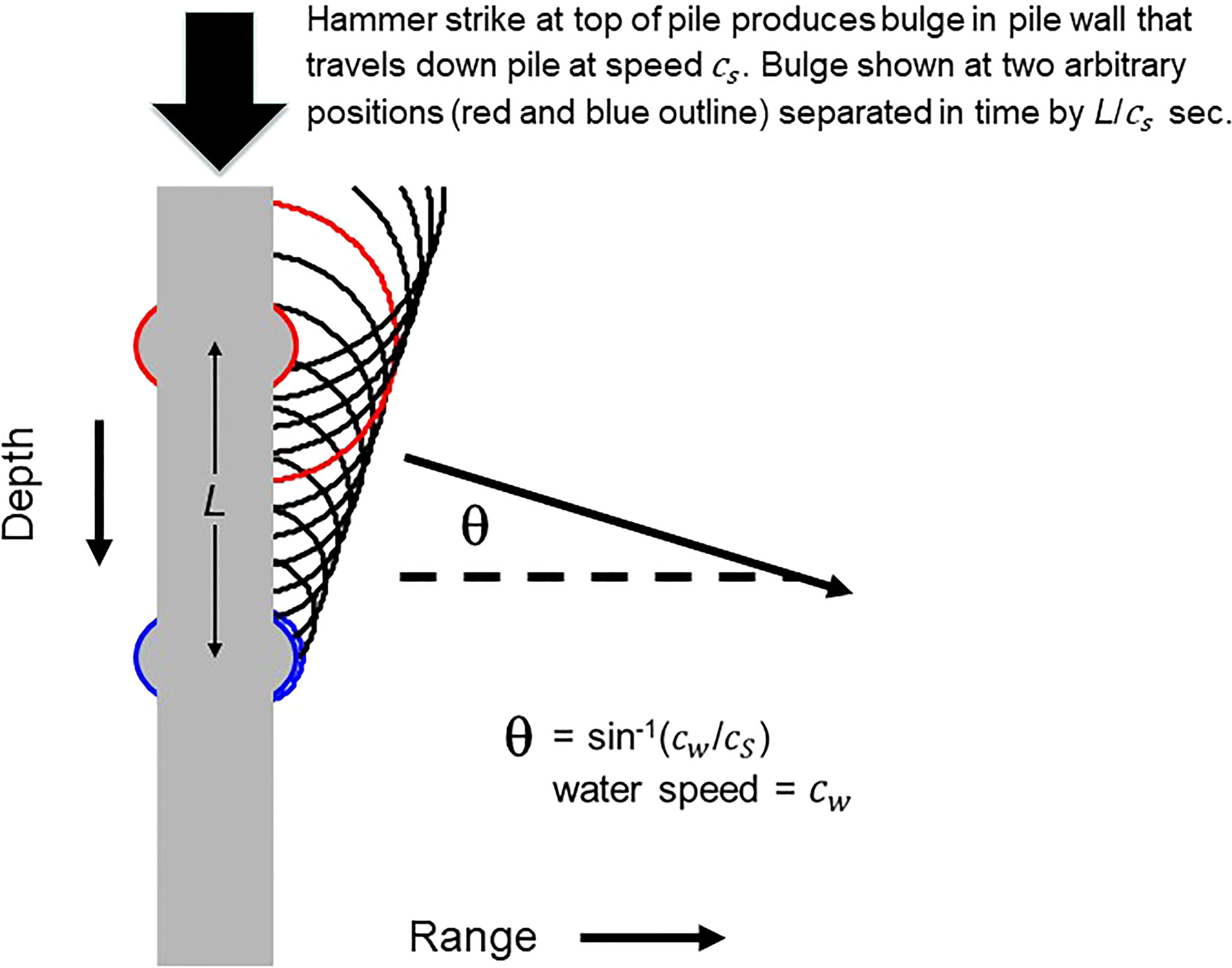
Figure 1 Bulge in the pile wall (red outline) as result of impact hammer strike (symbolized by large arrow) and subsequent compression of pile material. The bulge, which acts as a source of sound, travels down the pile at speed $c_s$ and is shown again having traveled a distance $L$ (blue outline). Wave fronts from the earlier emission (red) and later emission (blue) are shown with all prior emissions (black); these adding to form a quasi-planar wave front characterized by angle ${\theta }_m$. Modified from Dahl et al. (2015) with permission of the Acoustical Society of America, Copyright 2015, Acoustical Society of America.

The deformation or radial expansion continues traveling to the end of the pile where it reflects, and now acts as a sound source traveling upward on the pile surface. Upon reaching the top of the pile, a further reflection generates a second downward traveling source. This downward source is in effect approximately $T$ s after the first, where $T$ is twice the travel time of the deformation over the length of the pile. Although this is an idealized description, we show subsequently that key features of the Mach wave in terms of ${\theta }_m$ and time delay $T$ are observable.

3 Overview of measurement geometry and conditions

The measurements were made at the Washington State Ferries Eagle Harbor maintenance facility, located on Bainbridge Island (Puget Sound) in Washington State on October 31, 2005, to assess the effectiveness of a bubble curtain attenuation protocol for potential use in impact pile driving at ferry docks and other marine construction sites within Puget Sound. Further details on the study are summarized in the report by MacGillivray and Racca (2005), which determined that the attenuation protocol produced a reduction of approximately 10 dB in both acoustic pressure and velocity fields when mitigation was applied.

The 2005 study was based on measurements made from 10 piles (Figure 2), all piles being in place during the measurements, having been pre-inserted and extending approximately 5 m above the water line (the stated water depth of 10 m is assumed to apply to the entire area in Figure 2). The piles were typical steel piles frequently used in Puget Sound marine construction, of length $\sim$ 23.5 m, outer diameter 0.762 m, and wall thickness 0.019 m. The 2005 acoustic measurements covered the phase of impact pile driving used to drive the piles into the final $\sim$ 1.5 m of seabed substrate using a Delmag 62 single-action diesel impact hammer with a 14,600 lbs (6620 kg) hammer piston. This new study is limited to the two piles at range 10 m (T8) and 16 m (T5) during which the bubble attenuation protocol was not applied, as analyzing the effects of bubble mitigation is beyond the scope of this work.

FIGURE 2

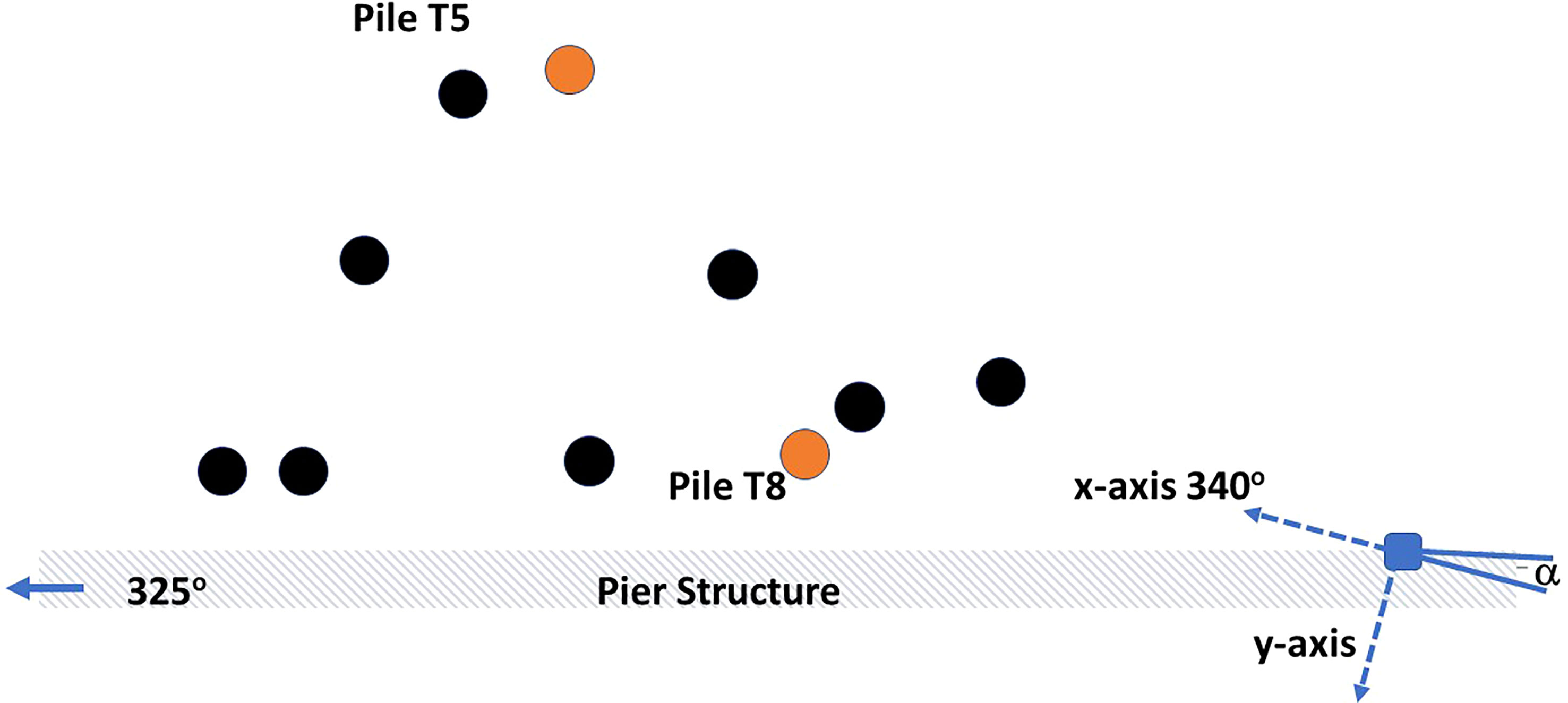
Figure 2 Location of the two piles T5 and T8 (orange circles) with respect to the acoustic measurement system (blue square) and the pier structure. For length scale reference the range from T8 to measurement system is 10 m. Bearing of T5 is ${355}^{\circ }$ and that of T8 is$335^{\circ }$. Other pile structures (black circles) shown in approximate relative position. The $x$-axis of the measurement system is pointing the direction ${340}^{\circ }$, $z$- axis (not shown) points upward. The angle $\alpha$ as shown is defined as positive with respect to the $x$-axis.

It is evident that the measurement geometry for piles T5 and T8 likely admitted multiple reflection and scattering from other piles and dock structures; the geometry is nevertheless representative of the kind of marine construction zone where often environmental monitoring must be undertaken. An additional complexity applies to pile T8 insofar as the bubble curtain apparatus surrounding the pile, though not operating, was in place for this measurement. The apparatus consisted of a 1 in. thick cylindrical PVC sleeve, 44 ft. long and 47 in. outside diameter, into which air was injected through two internally mounted aerating tubes.

Puget Sound archival shallow-water data for this time of year places water temperature² and salinity at $\sim$$10^{\circ }$ C and 28.5 ppt ³, respectively, from which sea water sound speed $c_w$ is estimated to be 1482 m/s. A sea water density ${\rho }_w$ of 1027 kg/ $m^3$ will be assumed.

3.1 Vector acoustic measurements

The acoustic pressure and velocity was measured by the pressure gradient method using a custom built, multi-component hydroacoustic sensor. The pressure gradient sensor was composed of a tetrahedral frame (Figure 3) supporting four Reson TC4043 hydrophones of sensitivity -201 dB re V/$\mu$Pa, along with an attitude/depth sensor. The hydrophones were cross-calibrated before and after the field measurements using a swept reference signal (from 100 Hz to 2 kHz) from an underwater loudspeaker. The four hydrophone channels were coherently sampled at individual channel sampling frequency of 25,000 Hz.

FIGURE 3

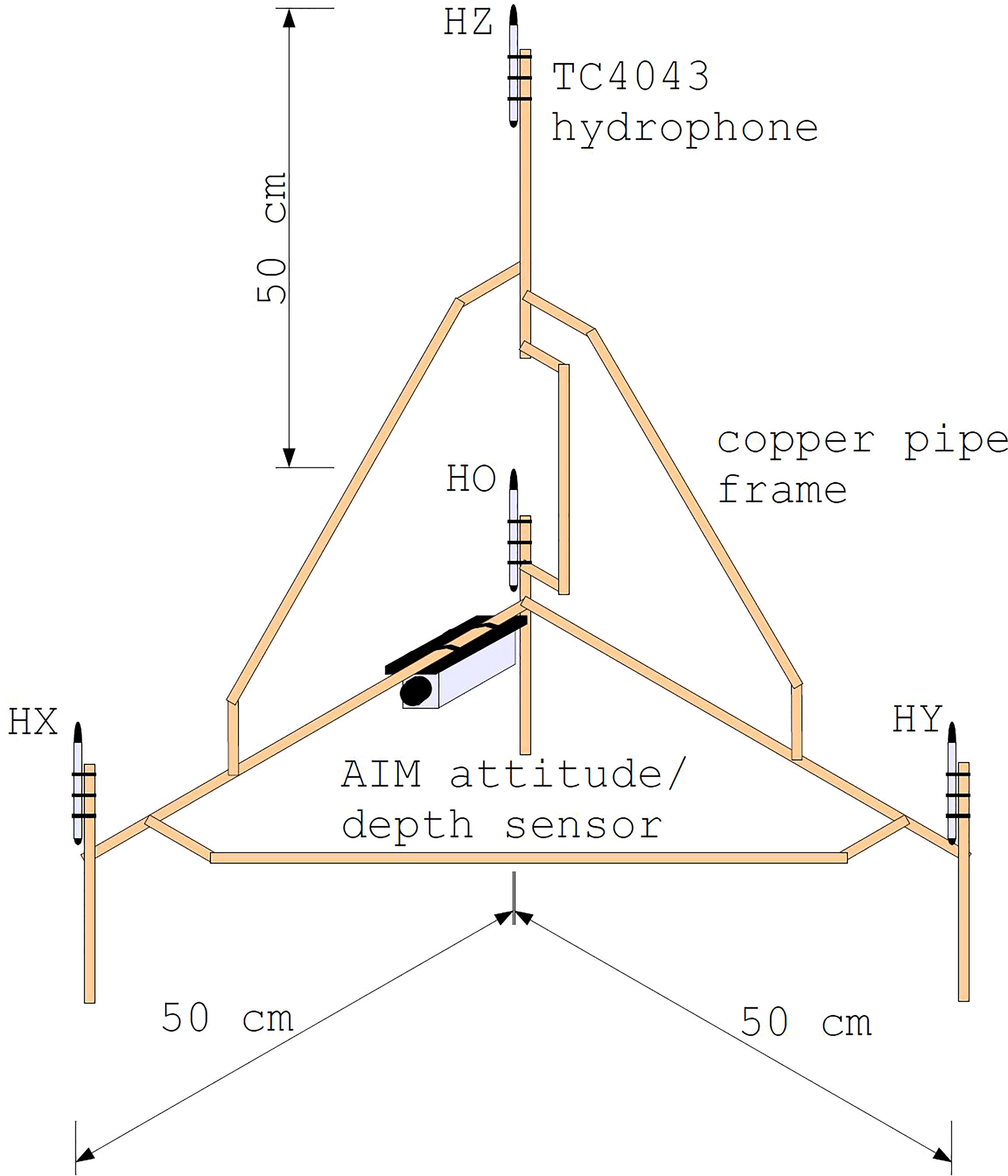
Figure 3 Schematic diagram of the pressure gradient sensor shown in isometric projection. Four Reson TC4043 hydrophones are located at the positions indicated $HO$ (origin) $HX$($x$-axis) $HY$($y$-axis) and $HZ$($z$-axis). The JASCO AIM attitude/depth sensor is oriented in the $x$-direction. The axial hydrophones $HX,HY$ and $HZ$ are all located 50 cm from the origin hydrophone $HO$.

The tetrahedral frame system was free to move but stable for the measurements from T5 and T8 (taken within an hour), for which the important orientation of the horizontal $x$-axis was determined by the attitude sensor to be $\sim$$340^{\circ }$, and thus $y$-axis was $\sim$$250^{\circ }$ (Figure 2), and the $x,y$ plane was at a depth 5 m.

To obtain kinematic quantities (acoustic acceleration and velocity) from this system, the finite difference approximation is used to estimate the acoustic pressure gradient. For example, the $x$-component of acoustic acceleration $a_x$ is derived from the $x$-component of the gradient as result of Euler’s equation,

$\begin{array}{ll}{a}_x=-\frac{1}{{\rho }_w}\frac{\partial p}{\partial x},& (1)\end{array}$

where ${\rho }_w$ is sea water density.

The finite difference approximation [5] yields an estimate of the acoustic pressure gradient through subtraction of pressure signals between the closely spaced hydrophones in Figure 3 labeled $HX,HY,HZ$, all separated from hydrophone $H0$ by $\text{Δ}=0.5$m. Thus an approximation to the acoustic pressure gradient in the $x$-direction, and hence $a_x$, is obtained from the difference of pressure signals $H0$ and $HX$,

$\begin{array}{ll}{a}_x\approx -\frac{1}{{\rho }_w}\frac{H0-HX}{\Delta }& (2)\end{array}$

where it is important that these signals are expressed in MKS units of Pa. The analogous operation yields estimates of the $y$- and $z$-components of acoustic acceleration $a_y$ and $a_z$, respectively, and corresponding estimates of acoustic velocity $v_{x,y,z}$ are obtained through time integration of $a_{x,y,z}$. For acoustic pressure $p$ the average (finite sum) of the four hydrophones is used, where

$\begin{array}{ll}p=(H0+HX+HY+HZ)/4.& (3)\end{array}$

All quantities in Eqs. (1-3) are assumed to be a function of time $t$.

Systematic errors arise from applying the finite difference (and sum) approximation to obtain both kinematic and dynamic (pressure) fields, stemming primarily from the length scale of the sensor separation $\text{Δ}$ with respect to the acoustic wavelength $\lambda$ Fahy (1995); Jacobsen and Juhl (2013), with both described by the parameter $k\text{Δ}$, where $k$ is the acoustic wavenumber.

Importantly, the normalized error in pressure $p$ ultimately becomes greater than that for velocity $v_{x,y,z}$, with direction for both quantities being such that approximate values (finite difference and finite sum) are less than true counterparts. This translates to estimates of velocity-based kinetic energy being greater than pressure-based potential energy for either frequency ranges or separations $\text{Δ}$ that put $k\text{Δ}$ above an acceptable value.

Small errors are also associated with the fact that the geometrical center of this 3D probe, where acoustic pressure $p$ is to be identified, is not co-located with the velocity components $v_{x,y,z}$. Nevertheless, simple formulas in Fahy (1995) for 1D probes give approximate guidance. To mitigate this error we limit the upper frequency range of the analysis to 710 Hz, representing a normalized separation of $k\text{Δ}<1.5$. At the upper end of this frequency range the kinetic energy level is expected to be approximately 1.5 dB greater than potential energy, for otherwise equal energies. This high-frequency limit is somewhat more conservative than that imposed in the original 2005 study. However, there remain additional tradeoffs that are specifically identified in Section 4.3. Additionally, for very low frequencies there can be errors in realizing the proper phase relation between pressure and velocity (Thompson and Tree, 1981) particularly if the measurements are from sources more complex than a single point source or monopole. We thus limit the low frequency range to $k\text{Δ}>0.1$, which translates to a low-frequency limit of $\sim$ 50 Hz. Imposing this limit does not produce further tradeoffs.

4 Analysis and results

4.1 Basic overview of time series

A summary of the 10-m (pile T8) and 16-m (pile T5) range measurements is presented in Figures 4 and 5. The pile strikes occur almost precisely every 1 s, and a short time series (0.075 s) $p_n(t)$ representing the $n^{th}$ strike in the series of $N$ is extracted by thresholding the pressure data to establish the onset time of a single strike arrival above background. The same onset time is applied to the velocity data for the corresponding time series $v_{{(x,y,z)}_n}(t)$ to maintain coherency between pressure and velocity channels. For pile T8 $N=$ 13 strikes, and for pile T5 $N=$ 24 strikes.

FIGURE 4

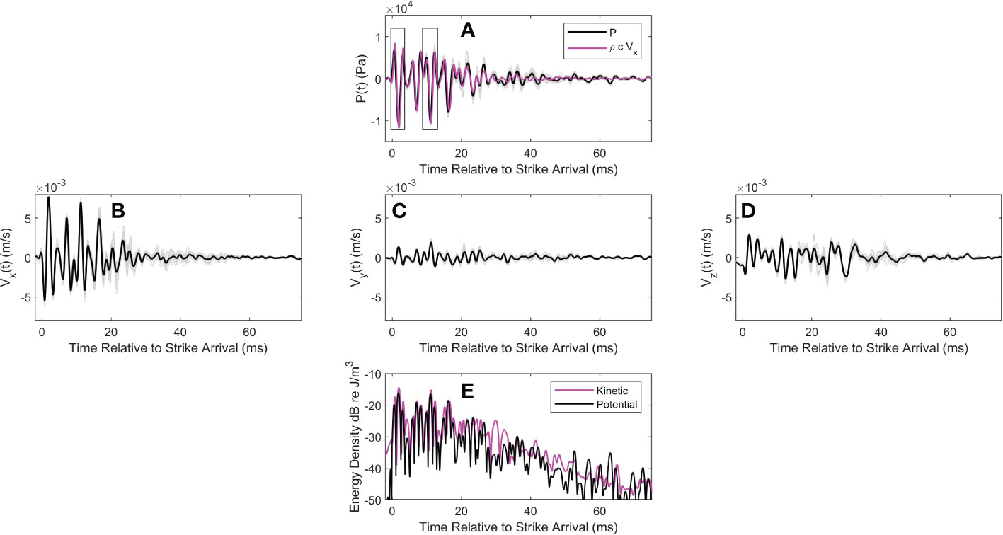
Figure 4 (A) coherent average of pressure over $N$ strikes $\overline{p}(t)$ (black line) and individual strike time series $p_n(t)$ (gray lines). Measurements are from pile T8 at range 10 m. Magenta line shows coherent average of the $x$ -component of acoustic velocity ${\overline{v}}_x(t)$ scaled by ${\rho }_w{c}_w$. For this display the sign of ${\overline{v}}_x(t)$ is flipped. Data shown within the two boxes (duration 4-ms) are used in subsequent analysis. Time is relative to the pile strike arrival. (B) Coherent average of ${\overline{v}}_x(t)$ along with individual strike time series $v_{x_n}(t)$ (gray lines); (C, D) provide similar display of ${\overline{v}}_y(t)$ and ${\overline{v}}_z(t)$, respectively, together with the individual strike time series (gray lines). (E) Time varying potential (black line) and kinetic (magenta line) energy density averaged over $N$ strikes.

FIGURE 5

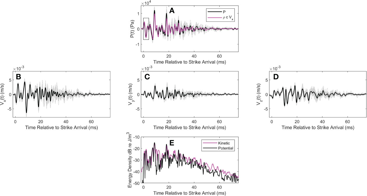
Figure 5 (A) coherent average of pressure over $N$ strikes $\overline{p}(t)$ (black line) and individual strike time series $p_n(t)$ (gray lines). Measurements are from pile T5 at range 16 m. Magenta line shows coherent average of the $x$-component of acoustic velocity ${\overline{v}}_x(t)$ scaled by ${\rho }_w{c}_w$. For this display the sign of ${\overline{v}}_x(t)$ is flipped. Data shown within the box (duration 4-ms) are used in subsequent analysis. (B) Coherent average of ${\overline{v}}_x(t)$ along with individual strike time series $v_{x_n}(t)$ (gray lines); (C, D) provide similar display of ${\overline{v}}_y(t)$ and ${\overline{v}}_z(t)$, respectively, together with the individual strike time series (gray lines). (E) Time varying potential (black line) and kinetic (magenta line) energy density averaged over $N$ strikes.

The coherent average of pressure, $\overline{p}(t)$, of the extracted time series over the $N$-strikes is

$\begin{array}{ll}\overline{p}(t)=\frac{1}{N}{\displaystyle \sum _{n=1}^N}{p}_n(t)& (4)\end{array}$

(black curves, Figures 4A and 5A). The same coherent average over the $N$ strikes is carried out for the three components of acoustic velocity yielding ${\overline{v}}_{x,y,z}(t)$ (black curves, Figures 4B–D and 5B–D). Individual strike time series (i.e., $p_n(t)$ and $v_{{(x,y,z)}_n}(t)$) are displayed by light gray lines and give a sense of the variation of strike arrival structure that tends to increase with time, presumably owing to the multiple scattering and reflection processes that are expected in this busy marine construction environment with nearby pier support structures, standing piles and floating construction barges.

The first arrival of approximately 4 ms displays less variation and is identified within a box (Figures 4A, 5A). This arrival is used subsequently for an analysis of the arrival angle, expected to be negative relative to horizontal and associated with the Mach wave. For pile T8 (Figure 4A) a second, 4 ms box is placed $T\sim$ 9.4 ms after the first arrival, which we postulate is associated with a second Mach wave characterized by the same arrival angle. The estimate of $T$ corresponds to the round-trip travel time of the deformation/source given a pile length of 23.5 m and speed $c_s\sim$ 5000 m/s. Such a second arrival for pile T5 is more difficult to identify owing to the longer range (16 m) although the delay time $T\sim$ 9.4 ms is still manifested in the spectrum as is shown subsequently. That the first arrival for pile T5 is not of the highest amplitude is also noteworthy. The influence of the Mach wave is lessened [10] when the observation depth is less than $R\tan {\theta }_m$, where $R$ is horizontal range from the pile source. Taking ${\theta }_m$ as approximately ${17}^{\circ }$ puts the measurement depth of 5 m on the edge of this bound.

For both piles the $x$-axis of the tetrahedral frame system was oriented most closely with the primary propagation path between pile source and receiver. It is thus of interest to plot acoustic velocity ${\overline{v}}_x(t)$ scaled by ${\rho }_w{c}_w$ (magenta line, Figures 5A and 6A). Note that the sign of ${\overline{v}}_x(t)$ is flipped in this display to facilitate a comparison in overlap between scaled velocity and pressure time series, but otherwise does not change the fact that the pressure and velocity are closely locked in phase and the acoustic field is primarily an active one. Looking ahead, the original sign of acoustic velocity will be important to preserve the correct direction of acoustic vector intensity.

FIGURE 6

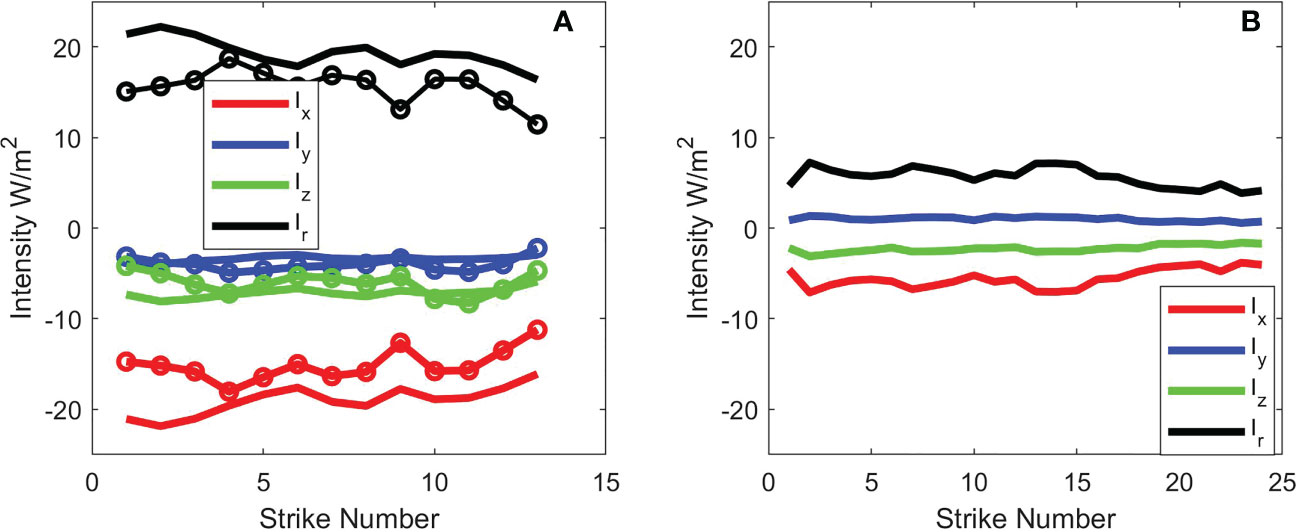
Figure 6 (A) Vector intensity Cartesian components $I_{{(x,y,z)}_n}$ and $I_{r_n}$ versus strike number $n$ derived from two selected arrival segments of the data from pile T8 at a range 10 m (see Figure 4A). First arrival identified by solid lines, and second (delayed by 9.4 ms) identified with same color code but with added symbols. (B) Same results corresponding to pile T5 range at 16 m (see Figure 5A), where only the first arrival is studied.

A final view is that of the ensemble average over $N$ strikes of potential $E_p(t)$ and kinetic $E_k(t)$ energy densities, where

$\begin{array}{ll}{E}_p(t)=0.5\frac{1}{N}{\displaystyle \sum _{n=1}^N\frac{p_n^2(t)}{{\rho }_w{c}_w^2}}& (5)\end{array}$

and

$\begin{array}{ll}{E}_k(t)=0.5\frac{1}{N}{\displaystyle \sum _{n=1}^N{\rho }_w(v_{x_n}^2(t)+v_{y_n}^2(t)+v_{z_n}^2(t)).}& (6)\end{array}$

The time varying potential (black line) and kinetic (magenta line) energy densities (Figures 4E, 5E) are expressed in dB re $\text{J}/m^3$, where it is evident that the majority of the energy arrives within the first 20 ms. For pile T8 (Figure 4E) a time-average of $E_k(t)$ and $E_p(t)$ over the first 20-ms equals $-$ 22.2 and $-$ 23.6 dB, respectively, and for pile T5 (Figure 5E) this same time-average equals $-$ 23.3 and $-$ 24.2 dB, respectively. In each case the kinetic exceeds the potential counterpart by 1 to 1.5 dB, which is in part consistent with chosen upper bound for $k\text{Δ}$ in applying finite difference approximation (Section 3.1). The notable excess in $E_k(t)$ over $E_p(t)$ near relative time 30 ms (Figure 4E) is very likely due to scattering from structures in close proximity of the receiving system, forming a near-field contribution. However, for both piles the average energy density in the remaining period from relative time 20 to 75 ms is approximately 10 dB less than that during the first 20 ms.

4.2 Vector intensity and arrival angles

The initial 4 ms of data denoted by the box (Figures 4A, 5A) represents a short-duration wavelet with initial positive-going pressure amplitude, and approximate center frequency $\sim$ 500 Hz. Let us denote a portion of the $p_n(t)$ and $v_{{(x,y,z)}_n}(t)$ time series over this same duration as $p_n(t_s)$ and $v_{{(x,y,z)}_n}(t_s)$, respectively. The active intensity in the $x$-direction (as defined by the reference frame Figure 2) for the $n^{th}$ strike, $I_{x_n}$, corresponding to this segment of the data equals the time average over duration $t_s$

$\begin{array}{ll}{I}_{x_n}=\langle p_n(t_s)v_{x_n}(t_s)\rangle .& (7)\end{array}$

The same operation involving $v_{y_n}(t_s)$ and $v_{z_n}(t_s)$ yields the active intensity in the $y$ and $z$-directions, or $I_{y_n}$ and $I_{z_n}$, respectively. For pile T8 this operation is also repeated on the second portion of data identified by the box delayed by 9.4 ms (Figure 4A).

The intensities $I_{{(x,y,z)}_n}$ estimated in this manner (Figure 6) tend to confirm the basic measurement geometry and are also approximately consistent with the Mach wave feature of impact pile driving. For pile T8 (Figure 6A), the sequence of $I_{x_n}$ and $I_{y_n}$ estimates for the first arrival are both negative, with the magnitude of $I_{x_n}$ being greatest; a result anticipated by inspecting the line-of-sight between T8 and the receiving system (Figure 2). Taking $I_x$ and $I_y$ as the average of the $N$-strike ensemble, the ratio $I_y/I_x\sim 0.18$ defines an angle $\alpha \sim {10}^{\circ }$ (Figure 2) and we infer the bearing of pile T8 is $\sim$$330^{\circ }$, with the direction of the active intensity vector in the horizontal plane being towards $\sim$$150^{\circ }$. For the second arrival delayed by 9.4 ms, (Figure 6A, same color code with added symbols) the ratio $I_y/I_x$ is slightly higher at $\sim 0.26$ indicating the T8 bearing is $\sim$$325^{\circ }$, but there is also considerably more variation. For pile T5 (Figure 6B), the sequence of $I_{y_n}$ estimates for the first arrival is positive, and that for $I_{x_n}$ is negative, with ratio $I_y/I_x\sim -0.18$ putting angle $\alpha \sim -{10}^{\circ }$. This is also consistent with the line-of-sight between pile T5 and the receiving system, and we infer the bearing of T5 is $\sim$$350^{\circ }$ with direction of the active intensity vector in the horizontal plane being towards $\sim$$170^{\circ }$.

For pile T8 (Figure 6A) $I_{z_n}$ is negative for both the first and second arrival, which is also the case for the first arrival with pile T5 (Figure 6B), which we interpret as the correct sense of a downward propagating Mach wave along the lines suggested by Figure 1. Defining a mean horizontal intensity $I_r$ as $\sqrt{I_x^2+I_y^2}$ the ratio $I_z/I_r$ is similar, $\sim -0.38$, for all arrivals (first and second in Figure 5A and first in Figure 5B). This translates to an angle $\sim$$21^{\circ }$ below the horizontal, versus a theoretically expected angle ${\theta }_m$ given by $\stackrel{-1}{\sin }\frac{c_w}{c_s}$ or $\sim {17}^{\circ }$ characterizing the arrival of the quasi-planar Mach wave (Figure 1). The discrepancy may be attributed to uncertainty in the vertical alignment of the $z$-axis of the measurements, which is not resolvable retrospectively from this 17-year old data set. Notably though, the observed angle is the same for the two ranges of 10 and 16 m.

4.3 Exposure levels and spectral densities

In this section the time series (Figures 4 and 5) are assessed in terms of both dynamic (pressure-based) and kinematic (velocity-based) measurements. The single-strike sound exposure level (SEL) is defined as the time integral of $|p_n(t){|}^2$ expressed in dB re $1\mu$$\text{P}{a}^2$-s, for which the time integral for these data is from relative time 0 to 75 ms. For both piles the strike-averaged SEL equals 176.8 dB, based on the more restrictive band-pass filtering (50-710 Hz) mentioned previously. Removing this filtering increases the SEL by only $\sim$ 0.5 dB, with 90% of the energy carried by frequencies between 50 and 710 Hz, changing to 95% with upper bound at 1000 Hz, and to 98% with upper bound at 2000 Hz.

Two spectral densities are next defined, sharing the common property that the integral of the (one-sided) spectral density over frequency equals the time integral of the squared-magnitude of corresponding time-domain quantity. Define first a squared magnitude spectrum $|P_n(f){|}^2$ corresponding to each $p_n(t)$ (expressed for this purpose in $\mu$Pa), computed via FFT and normalized so that the integral of $|P_n(f){|}^2$ equals the single strike SEL in linear units, where $f$ is frequency ($\text{Δ}f=$ 14 Hz). The SEL spectral density $S_p(f)$ is an average spectrum defined as

$\begin{array}{ll}{S}_p(f)=\frac{1}{N}{\displaystyle \sum _{n=1}^N}|P_n(f){|}^2.& (8)\end{array}$

The SEL spectral densities for the two piles (Figures 7A, 8A) each show peaks separated notionally by $1/T=106$ Hz (within the available spectral resolution), where $T\sim$ 9.4 ms represents the travel time of the deformation over twice the length of the pile. Integrating $S_p(f)$ over frequency recovers the strike-averaged SEL values listed above upon conversion to dB.

FIGURE 7

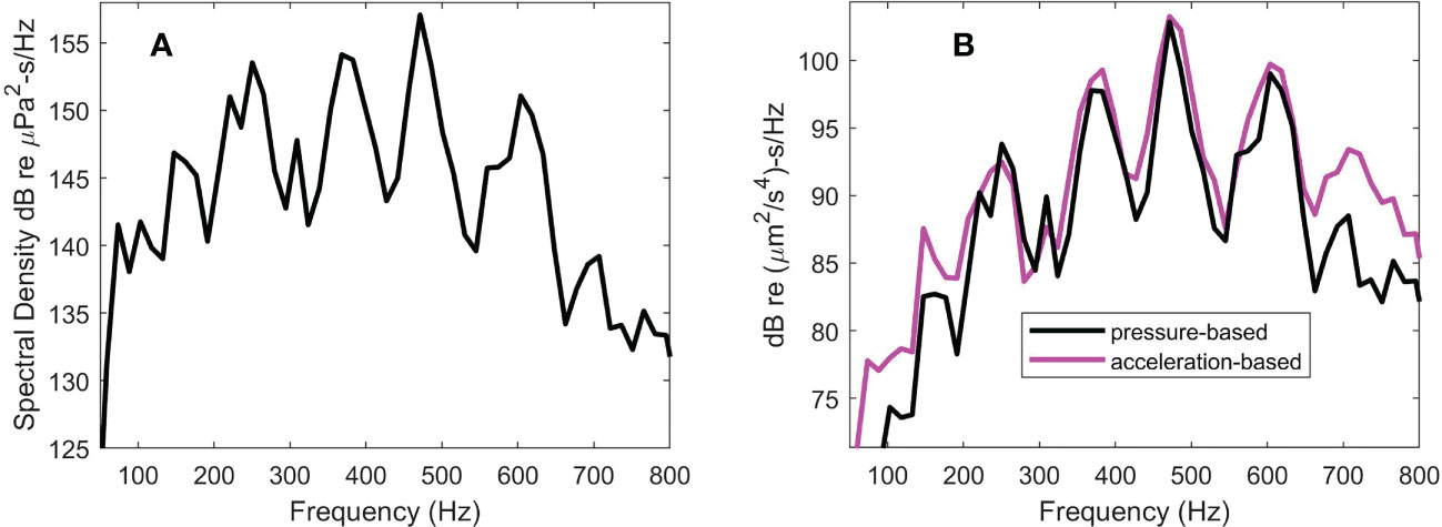
Figure 7 Spectral densities for pile T8, range 10 m (A) Sound exposure level (SEL) spectral density $S_p(f)$ (B) Acceleration exposure spectral density as derived with pressure data $A_p(f)$ (black line) and velocity data $A_k(f)$ (magenta line).

FIGURE 8

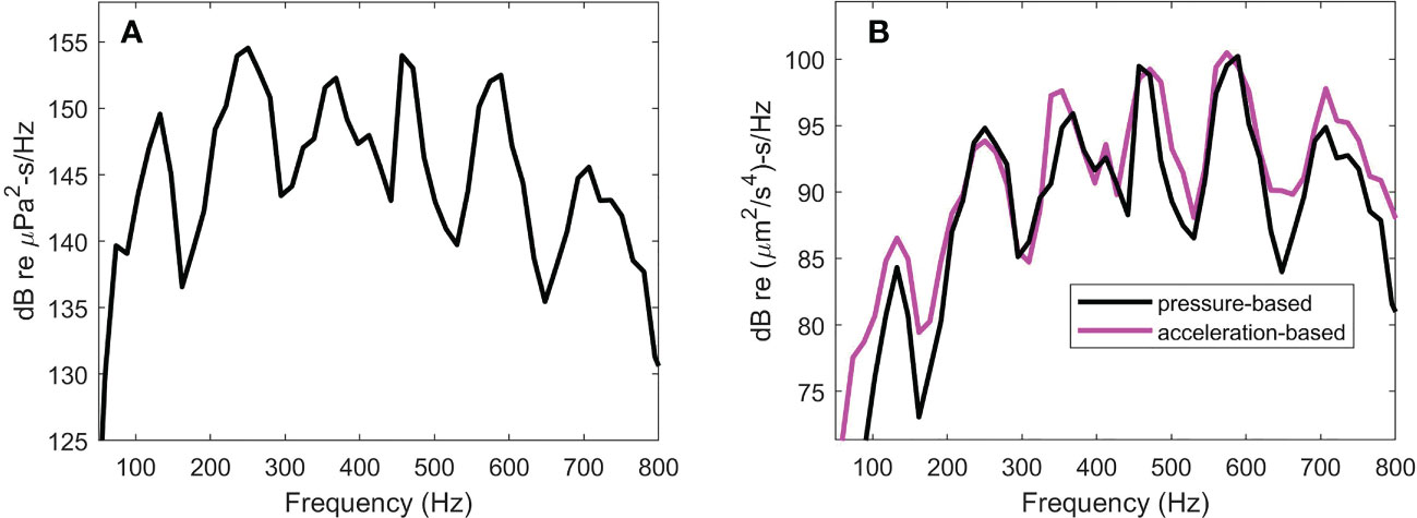
Figure 8 Spectral densities for pile T5, range 16 m (A) Sound exposure level (SEL) spectral density $S_p(f)$ (B) Acceleration exposure spectral density as derived with pressure data $A_p(f)$ (black line) and velocity data $A_k(f)$ (magenta line).

Somewhat analogous to $S_p(f)$ (with exception that MKS units are maintained) let us define $S_k(f)$ based on the velocity data, which is composed of three additive components $S_{k_x}(f)$, $S_{k_y}(f)$ and $S_{k_z}(f)$. A one-sided magnitude spectrum $|V_{xn}(f){|}^2$ is first computed corresponding to $v_{x_n}(t)$ and normalized so that the frequency integral of $|V_{xn}(f){|}^2$ equals the time integral of $\left|v_{x_n}(t){|}^2\right|$ of dimension$(\text{m}/\text{s}{)}^2$-s. An average spectrum based on $N$ strikes associated with the $x-$ component $S_{k_x}(f)$ is defined as

$\begin{array}{ll}{S}_{k_x}(f)=\frac{1}{N}{\displaystyle \sum _{n=1}^N|V_{xn}(f){|}^2.}& (9)\end{array}$

The analogous computation is performed for the $y$- and $z$- components producing $S_{k_y}(f)$ and $S_{k_z}(f)$, respectively.

The two spectral forms based on pressure and velocity data are next converted to acoustic acceleration exposure spectral density expressed in units of $m^2$$/s^4$ s/Hz, defining this spectral density derived from the kinematic data as $A_k(f)$ and that from pressure or dynamic data as $A_p(f)$. In terms of the kinematic data let $A_{k_x}(f)$ be the component of spectral density covering the exposure associated with the $x$-direction, where

$\begin{array}{ll}{A}_{k_x}(f)=S_{k_x}(f){(2\pi f)}^2.& (10)\end{array}$

The analogous conversion is made for the $y$- and $z$- components, $A_{k_y}(f)$ and $A_{k_z}(f)$, respectively, with three components summed to yield an estimate of $A_k(f)$. For the spectrum $A_p(f)$ using the pressure data, the conversion is

$\begin{array}{ll}{A}_p(f)={10}^{-12}\frac{S_p(f)}{{({\rho }_w{c}_w)}^2}{(2\pi f)}^2& (11)\end{array}$

where ${10}^{-12}$ is used to restore $S_p(f)$ to units of $\text{P}{a}^2$/Hz.

The two versions of these spectra (Figures 7B, 8B) again show peaks separated notionally by $1/T$ Hz. Note that the spectra are plotted with 120 dB offset to correspond to units of dB re $\mu$$m^2$$/s^4$ s/Hz, representing usage that is consistent with published studies on the effects of underwater noise on marine life, e.g., as in the work by Davidsen et al. (2019) on the effects of sound exposure from a seismic airgun. Analogous to SEL, the frequency integral of $A_k(f)$ yields an acceleration exposure level (AEL) in dB re $\mu$$m^2$$/s^4$s. The strike-averaged AEL is 122.9 dB for pile T8 at range 10 m and is 121.9 dB for pile T5 at range 16 m. Upon using the corresponding pressure-derived $A_p(f)$ the AEL reduces by $\sim$ 1.5 dB for pile T8 and $\sim$ 1 dB for pile T5.

Although agreement between the two AEL measures is satisfactory to within any reasonable calibration uncertainty, it is important in this case to consider the effect of limiting the upper frequency range to 710 Hz, necessary to realize the $k\text{Δ}<1.5$ bound. The factor $(2\pi f^2)$ in Eqs. (10) and (11) will amplify higher frequencies, which increases AEL if higher frequencies are included in the frequency integral. The effect can be assessed with the pressure data and $A_p(f)$. For example, using the same 95% energy criterion, AEL increases by 1 dB upon inclusion of frequencies up to 1000 Hz, and by 2 dB using 98% energy criterion involving frequencies up to 2000 Hz.

5 Discussion and summary

Vector acoustic properties of the underwater noise measured within the water column and originating from impact pile driving on steel piles has been studied, including the identification of features of Mach wave radiation associated with the radial expansion of the pile upon hammer impact. The data were recorded on a four-channel hydrophone system mounted on a tetrahedral frame at a depth of 5 m in waters 10 m deep. The system measured acoustic pressure and, using the finite difference approximation, measured the gradient of acoustic pressure in three dimensions (hydrophone separation $\text{Δ}=$0.5 m) from which estimates of kinematic quantities, such as acoustic velocity and acceleration exposure spectral density, were derived.

The 2005 study from which these data originate was conducted at a marine construction site in Puget Sound with the primary purpose to assess effectiveness of a bubble curtain attenuation protocol. The two piles, T8 at range 10 m and T5 at range 16 m (Figure 2), selected for this study were not subjected to the bubble-mediated mitigation; however, a bubble curtain apparatus consisting of a cylindrical PVC sleeve (though not operational) still surrounded the closer T8 pile. It is likely for this reason that the strike-averaged SEL measured at the closer T8 pile was approximately identical to that estimated at the more distant T5 pile, both $\sim$ 177 dB re $1\mu$$\text{P}{a}^2$-s.

To mitigate errors associated with use of the finite difference approximation, the data were band-passed filtered between 50 and 710 Hz, equivalent to placement of $k\text{Δ}$ between 0.1 and 1.5, where $k$ is acoustic wavenumber. The upper bound $ka$ was chosen to limit to 1.5 dB the discrepancy between otherwise equivalent dynamic (pressure based) and kinematic quantities. In terms of the pressure-only data, removal of such filtering increased SEL by approximately 0.5 dB.

For each pile the initial 4 ms segment of pressure and velocity waveform data (boxes starting at relative time 0, Figures 4A, 5A) was selected for more detailed analysis. Evidence of the fidelity of the estimated 3-component acoustic velocity was shown by the accuracy with which the pile bearing with respect to the receiver location (Figure 2), was recovered from the ratio of active intensities in the $x$ and $y$ directions. For pile T8 a second data segment, delayed by $T=$ 9.4 ms, was selected from which the approximate bearing was also reliably recovered. The 9.4 ms delay equals the travel time of the deformation (radial expansion) over twice the length of the pile.

The time varying potential $E_p(t)$ and kinetic $E_k(t)$ energy densities over the entire 75 ms of waveform time series data (Figures 4E, 5E) was also studied with results showing that the majority of the energy arrives within the first 20 ms. Time-averages of $E_k(t)$ over the first 20-ms for piles T8 range 10 m and T5 range 16 m yielded values $-$ 22.2 and $-$ 23.3 dB re $\text{J}/m^3$, respectively, with the corresponding time averages of $E_p(t)$ being $\sim$ 1 to 1.5 dB less. These differences are reasonably consistent with the expected energy difference (1.5 dB) based on the chosen upper bound for $k\text{Δ}$ used in the finite difference approximation. Some degree of excess of $E_k(t)$ over $E_p(t)$ was observed particularly in later portions of the time series (beyond 20 ms) that is likely the result of near field effects due to secondary (scattering) sources such as other piles and dock structures in close proximity to the receiving system, although the average kinetic energy density over the remainder of the time series from 20 to 75 ms is approximately 10 dB less than that computed over the initial 20 ms.

Using the same selection of waveform data (boxes Figures 4A, 5A) the ratio of active vertical (in the $z$ direction) to horizontal intensity yielded a notionally correct angle, directed downward with respect to horizontal and indicative of the expected quasi-planar Mach wave produced in impact pile driving. The accuracy of this angle is limited owing to instrumental uncertainty in the vertical orientation of the measurement frame; importantly, however, the determined angle was approximately the same for the two ranges, which is consistent with an expected property of the Mach wave. It is also worth noting that, unlike the case for pile T8 at range 10 m, the initial 4 ms of data for pile T5 at range 16 m did not have the highest amplitude relative to the remainder of the time series. A plausible reason is that amplitude of the downward Mach cone diminishes for depths less than $R\tan {\theta }_m$ where $R$ is range (see (Reinhall and Dahl (2011)). The 5-m measurement depth begins to satisfy this criterion at range 16 m. More definitive interpretation of the time series data in Figures 4 and 5 beyond these basic observations is made difficult by the likely presence of multiple reflection and scattering of the acoustic field from other piles and dock structures, which is not uncommon for the type of busy marine construction zone where often environmental acoustic monitoring must be undertaken.

Of greater interest, however, are two variations of spectral densities (Figures 7 and 8) each based on the full extent of waveform data displayed in Figures 4 and 5. Evident in each spectra are peaks separated by $\sim 106$ Hz, or $1/T$, representing a clearly observable manifestation of the Mach wave embodied in the spectra. Furthermore the active, propagating nature of the acoustic field, such as evidenced by the ${\rho }_w{c}_w$ scaling in Figures 4A,5A, motivated comparisons between the pressure-based and velocity-based spectra.

From a comparison of acceleration exposure spectral density (Figures 7B, 8B), it is evident that the two forms $A_p(f)$ based on pressure, and $A_k(f)$ based on the three components of acoustic velocity, are in notional agreement. Computing from these, the acceleration exposure level (AEL) in dB re $\mu$$m^2$$/s^4$-s yielded a strike-averaged AEL of 122.9 dB for pile T8 at range 10 m and 121.9 dB for pile T5 at range 16 m; the corresponding pressure-derived AEL estimates were 1 to 1.5 dB lower, and also consistent with the chosen upper bound for $k\text{Δ}$. However, AEL does increase upon including higher frequencies, and assessing this effect using the pressure data showed that using the same 95% energy criterion, AEL increases by 1 dB upon inclusion of frequencies up to 1000 Hz, and by 2 dB using 98% energy criterion involving frequencies up to 2000 Hz.

It is worth emphasizing that from the standpoint of environmental monitoring, vector acoustic measurements within the water column such as those discussed here are inherently more difficult to make than scalar sound pressure measurements. Apart from the additional data analysis requirements, the calibration effort for a vector sensing system is four times that of a single hydrophone, and likelihood for systematic errors necessarily expands. This effort does not include the additional collection of metadata to monitor the equipment’s orientation for resolving direction of the vector fields.

To study effects on marine life, acoustic data must be used as some measure of dosage from which a response is to be found. As a practical matter, any dose metric involving kinematic quantities (acoustic velocity, acceleration, displacement) must be in magnitude form as for example, in the AEL measure, and necessarily involve a degree of averaging. Here we have demonstrated, insofar as the finite difference approximation allows, the equivalence of observations based on dynamic (pressure) and kinematic components of the underwater acoustic field from impulse pile driving measured within the water column. The result should not be surprising given that such an acoustic field from impact pile driving is active and propagating energy, as distinct from a reactive field. This study nonetheless provides experimental evidence that may inform the choice of instrumentation in planning acoustic monitoring of pile driving operations.

Data availability statement

The data analyzed in this study is subject to the following licenses/restrictions: The raw data were gathered more than 17 years ago. Metadata is that identified only in this article. Information on processing of the raw data is that given only in this article. Requests to access these datasets should be directed to dahl@apl.washington.edu.

Author contributions

PD carried out the 2022 retrospective analysis contained herein on vector acoustic properties and produced the original draft of this manuscript along with figures associated data display and analysis. AM and RR conducted the original measurements in 2005 in cooperation with Washington State Department of Transportation (WSDOT), data analysis including the effects of bubble mitigation as documented in their 2005 report, and delivered the fully calibrated pressure and velocity data base to WSDOT archives used by PD, and contributed in the review and revision of the original draft. AM also evaluated and interpreted essential metadata used by PD. All authors contributed to the article and approved the submitted version.

Funding

The original data collection in 2005 was performed under a contract from the WSDOT. PD’s efforts were funded by the U.S. Office of Naval Research.

Acknowledgments

The efforts of Jim Laughlin of WSDOT are appreciated for his help in coordinating the WSDOT funded study and recovery of the 2005 data from WSDOT data archives.

Conflict of interest

Authors AM and RR are employed by JASCO Applied Sciences Canada Ltd.

The remaining author declares that the research was conducted in the absence of any commercial or financial relationships that could be construed as a potential conflict of interest.

Publisher’s note

All claims expressed in this article are solely those of the authors and do not necessarily represent those of their affiliated organizations, or those of the publisher, the editors and the reviewers. Any product that may be evaluated in this article, or claim that may be made by its manufacturer, is not guaranteed or endorsed by the publisher.

Footnotes

1. ^ https://www.boem.gov/environment/underwater-acoustic-monitoring-data-analyses-block-island-wind-farm-rhode-island
2. ^ https://www.seatemperature.org/north-america/united-states/bainbridge-island-october.htm
3. ^ www.eopugetsound.org

References

Dahl P. H., Dall’Osto D. R. (2020). Vector acoustic analysis of time-separated modal arrivals from explosive sound sources during the 2017 seabed characterization experiment. IEEE J. Oceanic Eng. 45, 131–143. doi: 10.1109/JOE.2019.2902500

CrossRef Full Text | Google Scholar

Dahl P. H., de Jong C. A. F., Popper A. N. (2015). The underwater sound field from impact ple driving and its potential effects on marine life. Acoustics Today 11, 18–25.

Google Scholar

Dahl P. H., Reinhall P. G. (2013). Beam forming of the underwater sound field from impact pile driving. J. Acoustical Soc. America 134, EL1–EL6. doi: 10.1121/1.4807430

CrossRef Full Text | Google Scholar

Davidsen J. G., Dong H., Linné M., Andersson M. H., Piper A., Prystay T. S., et al. (2019). Effects of sound exposure from a seismic airgun on heart rate, acceleration and depth use in free-swimming Atlantic cod and saithe. Conserv. Physiol. 7. doi: 10.1093/conphys/coz020

CrossRef Full Text | Google Scholar

Fahy F. (1995). Sound intensity. 2nd Ed (London, U.K: Chapman and Hall).

Google Scholar

Halvorsen M. B., Casper B. M., Woodley C. M., Carlson T. J., Popper A. N. (2012). Threshold for onset of injury in chinook salmon from exposure to impulsive pile driving sounds. PloS One 7. doi: 10.1371/journal.pone.0038968

CrossRef Full Text | Google Scholar

Jacobsen F., Juhl P. M. (2013). Fundamentals of general linear acoustics (Chichester, West Sussex, U.K: Wiley).

Google Scholar

MacGillivray A. (2018). Underwater noise from pile driving of conductor casing at a deep-water oil platform. J. Acoustical Soc. America 143, 450–459. doi: 10.1121/1.5021554

CrossRef Full Text | Google Scholar

MacGillivray A., Racca R. (2005). Technical report: Sound pressure and particle velocity measurements from pile driving at Eagle Harbor maintenance facility, bainbridge island, WA (Olympia, WA: Washington State Department of Transportation). Available at: https://wsdot.wa.gov/sites/default/files/2021-10/EnvNoiseMonRptEagleHarborPileDriving.pdf.

Google Scholar

Reinhall P. G., Dahl P. H. (2011). Underwater mach wave radiation from impact pile driving: Theory and observation. J. Acoustical Soc. America 130, 1209–1216. doi: 10.1121/1.3614540

CrossRef Full Text | Google Scholar

Thompson J., Tree D. (1981). Finite difference approximation errors in acoustic intensity measurements. J. Sound Vibration 75, 229–238. doi: 10.1016/0022-460X(81)90341-2

CrossRef Full Text | Google Scholar

Tsouvalas A. (2020). Underwater noise emission due to offshore pile installation: A review. Energies 13, 872–879. doi: 10.3390/en13123037

CrossRef Full Text | Google Scholar

Tsouvalas A., Metrikine A. V. (2013). A semi-analytical model for the prediction of underwater noise from offshore pile driving. J. Sound Vib 332, 3232–3257. doi: 10.1016/j.jsv.2013.01.026

CrossRef Full Text | Google Scholar

Zampolli M., Nijhof M. J. J., de Jong C. A. F., Ainslie M. A., Jansen E. H. W., Quesson B. A. J. (2013). Validation of finite element computations for the quantitative prediction of underwater noise from impact pile driving. J. Acoustical Soc. America 133, 72–81. doi: 10.1121/1.4768886

CrossRef Full Text | Google Scholar