Satellite to buoy IoT communications in the Arctic Ocean

1 Introduction

It is of increasing importance to place sensors anywhere on the earth that can report weather and climate parameters, which can aid operations in remote areas and report the climate status. IoT has gained significant importance when it comes to remote agriculture and maritime monitoring. Coverage to remote sensors may be attained using terrestrial mobile radio communications systems from earlier generations to 5G and in addition satellite systems. (Wei et al., 2020) gives an excellent comprehensive survey of hybrid terrestrial and satellite systems for IoT. Recently, several LEO systems have been proposed, see (Palma and Birkeland, 2018; Birkeland and Palma, 2019), which give a survey. The LoRa Alliance has initiated the LoRaWAN_TM 1.1 specification (LoRaWAN®, 2020), which is a network protocol suited for battery-powered, mobile-, or fixed end-devices. The access is radio based including mobile and fixed IoT devices accessing mobile network base stations. In 2020, the LoRa Alliance released the standard LoRaWAN of Regional Parameters RP2-1.0.2. using Frequency Hopping Spread Spectrum (FHSS) suited for LEO satellite systems. As such, the standard may serve as a hybrid access system to IoT devices. The 3rd Generation Partnership Project (3GPP) specifications include studies and requirements for 5G satellite access extending the 5G technology to non-terrestrial networks (3GPP, 2019). This reference gives a broad overview of both satellite only systems and hybrid satellite/terrestrial systems.

In our case, we limit the scope, which is described in the following. We focus on a geographical area that have little or no infrastructure to provide IoT. Hence, our focus and example area are the Arctic region in the North Atlantic. In the Arctic areas, which mostly consist of either open sea or an ice shelf, the communications to sensors must be provided by satellites. In some areas close, e.g., to Arctic islands, it is possible to use hybrid systems. However, in this presentation, we focus on IoT from buoys floating on the sea surface, far from land areas, and that must be powered locally, and where power is a limited resource. The GEO satellites cannot cover the highest latitudes (from 70°/80° to 90°), and satellite orbits that can cover all latitudes must be used. We will focus on LEO satellite systems that are orbiting at a height 400–2,000 km, and we have chosen 800 km in our analyses. The main advantages of LEO systems are that a) the round-trip latency is moderate ≈5–40 ms compared to GEO that is ≈250 ms, b) the free space loss have a gain compared to GEO of 30–40 dB, and c) a LEO satellite system can reach all latitudes. The main disadvantages are that a) the LEO system must have many satellites to cover the earth, b) there is a need for frequent handovers between satellites, and c) if only one satellite is used, communication is only possible in periods of the time and the orbit must be over the area supposed to be covered.

The World Radiocommunication Conference (WRC) 2019, resolution 248 (RESOLUTION 248 (WRC-19), 2019), established a new agenda for the WRC 2023, which will evaluate additional allocations for low data rate mobile satellite services. These services might be suitable for the IoTs in Arctic and oceanic regions. The candidate bands are as follows: (1,690–1,710 MHz, 2,010–2,025 MHz, 3,300–3,315 MHz, and 3,385–3,400 MHz). However, the WRC has stated that existing primary services in these bands creating interference must be investigated to see the suitability of these bands for low data rate services. In this paper, our primary focus is placed on the license-free UHF bands located at 433 MHz and 868 MHz, and the bands that were determined by resolution of 248 at the WRC 2019 mentioned above. Among these bands, we focus on the highest frequency band, which ranges from 3,385 MHz to 3,400 MHz.

Since 1983, Inmarsat GEO systems have included maritime distress and emergency systems and telephones. With the Inmarsat C standards, a low-rate data communication system launched in 1991 was accessible everywhere except for high latitude locations (above 75°–80° latitude). The Irridium LEO system was in operation from 2001 and has been utilized for telephony and short emergency message services in locations outside the reach of terrestrial mobile systems, and at high latitudes. Recent planning and launches of so-called mega satellite networks include the Canadian Telsat system, the OneWeb system, and SpaceX’s Starlink. Through their project ArcticCOM, ESA has addressed the lack of communications in the Arctic region.

Inaccessible marine or land areas present numerous difficulties for IoT sensor deployment. The sensors must be battery powered and powered either by micro-windmills or solar panels. The uplink communication will then become crucial. However, predicting the up-link budget will therefore depend on having thorough understanding of all propagation mechanisms that affect the received power at the satellite. A sensor on a sea buoy placed on the sea surface will display both large angular and linear movements due to the sea waves, which will be a challenge and guideline for the design of the antenna. For the buoy’s mechanical structure and the antenna subsystem, we have used a simple model defining the antenna’s center height above the sea level and an idealized antenna pattern explained later in the text. We believe that an adaptive antenna array design to account for the angular movement of the buoy may be challenging to design, due to power limitations and is currently not feasible. Except for the height above sea level, the mechanical design of the antenna is outside the scope of this study. Furthermore, the IoT type of data, sensors, QoS requirements, and capacity requirements for different applications are outside the scope as well.

The paper is organized as follows. In Section 2, we investigate the radio reflection phenomena from the sea surface surrounding a sensor mounted on an obstacle, e.g., a buoy, floating on the sea surface. These phenomena and their impact on the propagation loss is assessed. Furthermore, when the LEO satellite is viewed at a low elevation angle, diffraction loss caused by the round earth will occur and is included in the model. The latter is part of the Round Earth Loss model (Yang et al). We present and discuss the analysis results including these models. In Section 3, we discuss and evaluate ionospheric loss. These losses are frequency dependent, and we focus on frequencies mentioned above. Furthermore, we discuss the impact of losses due to precipitation and refraction in the troposphere. In Section 4, we perform link budget analysis. In the discussion, we include important factors of the buoy that are the available power, the antenna solution and antenna pattern, the movement of the buoy on the sea surface, and important radio parameters like EIRP and G/T under different conditions. Using the assessment of ionospheric and tropospheric losses, we include these in the link budget. The statistical issues of ionospheric loss are also discussed and assessed. Furthermore, some typical LEO radio data will be used in the analysis, like G/T and EIRP data for a LEO satellite. Link budget results for some scenarios are presented. Finally, in Section 5, we sum up the results and give some concluding remarks.

2 Reflection phenomena and the Round earth loss model

2.1 Satellite orbit and geometry with a buoy at the sea surface

Figure 1 depicts a LEO satellite rotating clockwise around the earth. On the earth’s sea surface, a buoy is located at point A. The figure depicts a cross-section of the earth through point A, the earth’s center CE, and in the satellite orbiting plane. We discuss and analyze the scenario in which the satellite becomes visible to point A at point HR, passes point A on the sea surface in zenith Z, and disappears in the horizon at point HS. This zenith passage of the satellite is the most advantageous situation for radio propagation to the buoy at A.

FIGURE 1

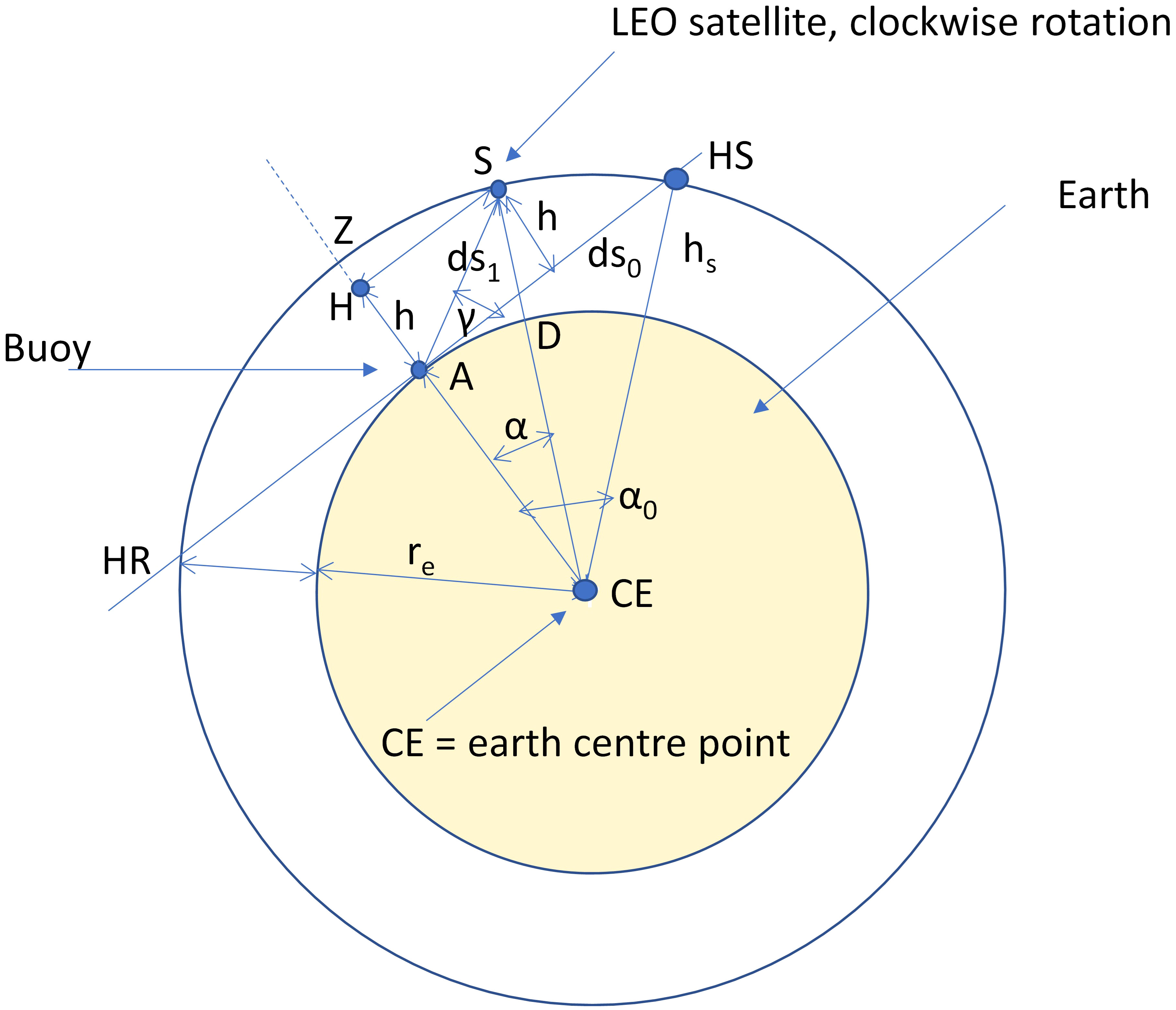
Figure 1 LEO satellite geometry with respect to an object on the sea surface.

A LEO orbit can have an altitude of 400–2,000 km and a cycle of 93–127 min. In Table 1, variables shown in Figures 1, 2 are defined.

TABLE 1

Table 1 Definition of variables shown in Figures 1, 2.

FIGURE 2

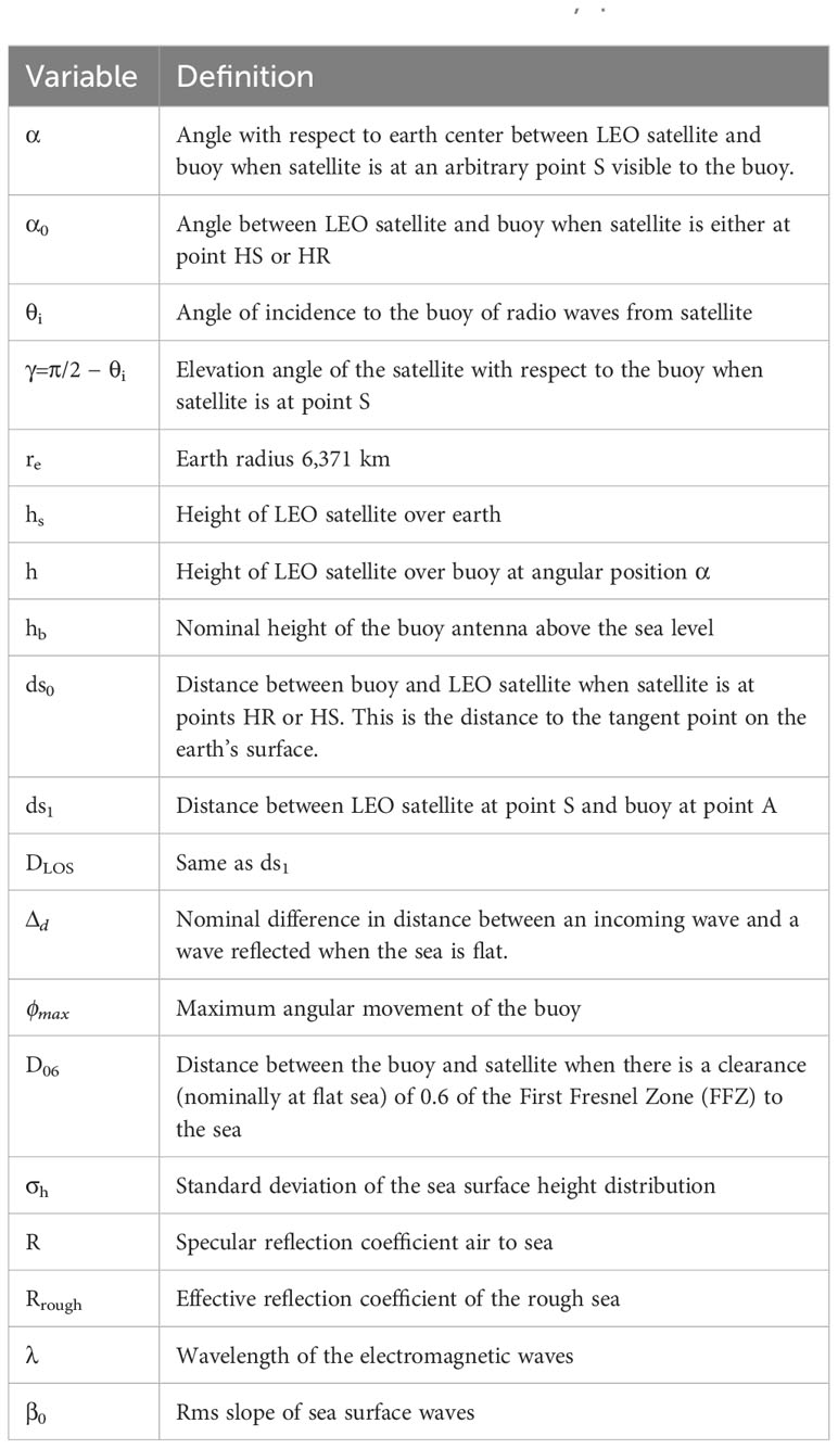
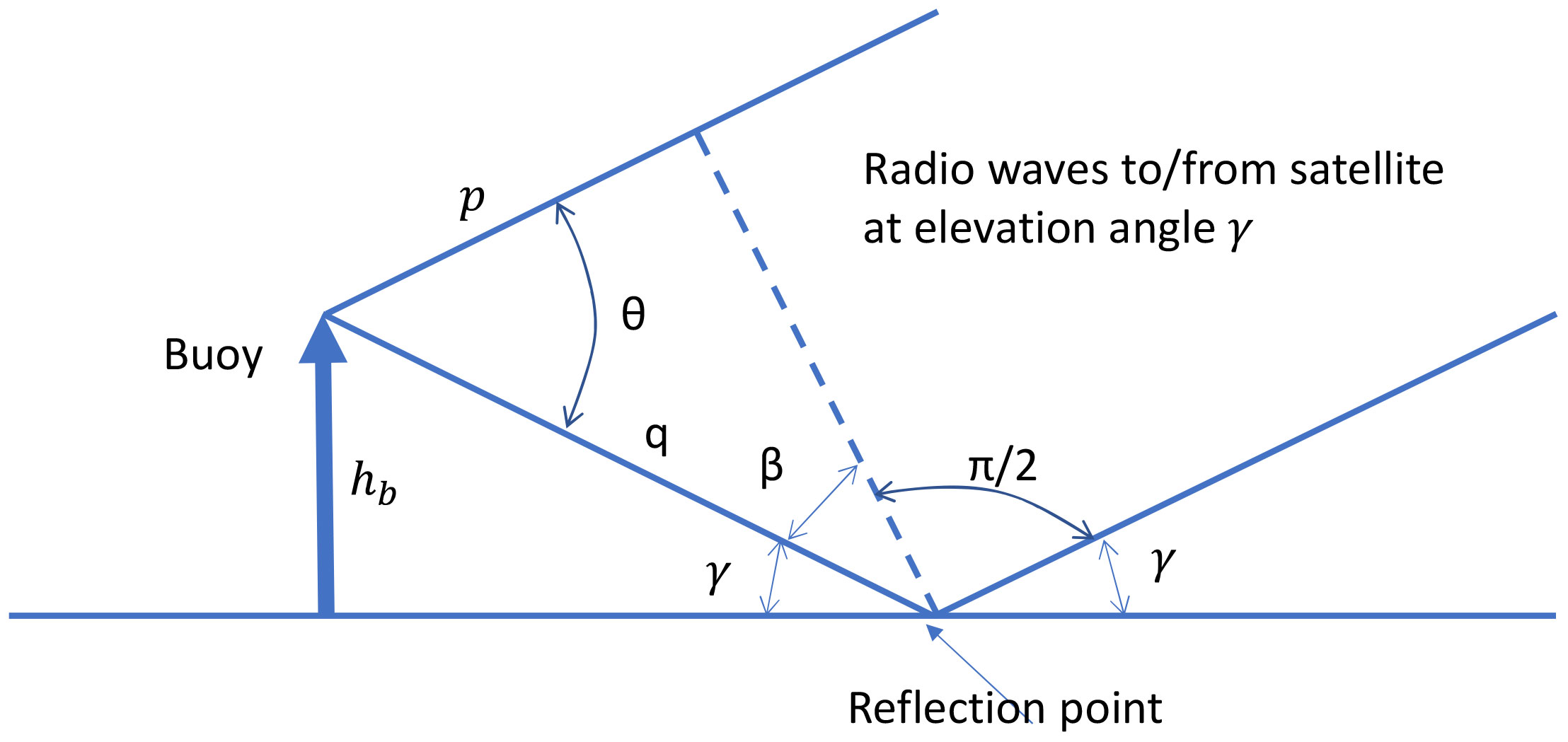
Figure 2 Reflection from the ideal flat sea at the buoy. The incoming waves are at an elevation angle γ.

The distance ds₀ between A and HS (and HR) is given by

$\begin{array}{ll}\begin{array}{c}\mathit{\text{d}}{\mathit{\text{s}}}_{\mathbf{0}}=\sqrt{{\left({\mathit{\text{h}}}_{\mathit{\text{s}}}\right)}^{\mathbf{2}}+\mathbf{2}{\mathit{\text{h}}}_{\mathit{\text{s}}}{\mathit{\text{r}}}_{\mathit{\text{e}}}}\end{array}& (1)\end{array}$

The angle a₀ is given by

$\begin{array}{ll}\begin{array}{c}{\mathit{\text{α}}}_0=\mathbf{\text{arccos}}(\frac{{\mathit{\text{r}}}_{\mathit{\text{e}}}}{{\mathit{\text{h}}}_{\mathit{\text{s}}}+{\mathit{\text{r}}}_{\mathit{\text{e}}}})\end{array}& (2)\end{array}$

The cosine rule on the triangle CE-S-A is used to calculate the distance ds₁ from point S to buoy at A

$\begin{array}{ll}\begin{array}{c}\mathit{\text{d}}{\mathit{\text{s}}}_{\mathbf{1}}=\mathit{\text{sqrt}}\left[{\left({\mathit{\text{r}}}_{\mathit{\text{e}}}+{\mathit{\text{h}}}_{\mathit{\text{s}}}\right)}^{\mathbf{2}}+{\mathit{\text{r}}}_{\mathbf{\text{e}}}^{\mathbf{2}}-\mathbf{2}·\left({\mathit{\text{r}}}_{\mathit{\text{e}}}+{\mathit{\text{h}}}_{\mathit{\text{s}}}\right)·{\mathit{\text{r}}}_{\mathit{\text{e}}}·\mathit{\text{cos}}\left(\mathit{\text{α}}\right)\right]\end{array}& (3)\end{array}$

The height h of the LEO satellite over buoy’s tangential plane at angular position α is

$\begin{array}{ll}\begin{array}{c}\mathit{\text{h}}=\left({\mathit{\text{h}}}_{\mathit{\text{s}}}+{\mathit{\text{r}}}_{\mathit{\text{e}}}\right)·\mathbf{\text{cos}}\left(\mathit{\text{α}}\right)-{\mathit{\text{r}}}_{\mathit{\text{e}}}\end{array}& (4)\end{array}$

The elevation angle γ of the satellite at position S with respect to the buoy is:

$\begin{array}{ll}\begin{array}{c}\mathit{\text{γ}}=\mathbf{\text{arcsin}}(\frac{\mathit{\text{h}}}{\mathit{\text{d}}{\mathit{\text{s}}}_{\mathbf{1}}})\end{array}& (5)\end{array}$

Equations 1–5 can be used to calculate relevant distances and angles for the Round Earth Loss (REL) model with the angle α as a parameter. Figure 3 to the left depicts the situation when the buoy is on a flat sea, while the figure to the right depicts the situation when the buoy is moving on sea waves. In the latter case, the buoy will move linearly and angularly in all linear and angular directions.

FIGURE 3

Figure 3 To the left: Incoming and reflected radio waves to the buoy, flat sea. To the right: moving buoy on sea waves.

The difference in distance Δ_d = q - p (see Figure 2) between the reflected radio wave and the direct wave in the flat sea situation is given by the expression:

$\begin{array}{ll}\begin{array}{c}{\text{Δ}}_{\mathit{\text{d}}}=\frac{{\mathit{\text{h}}}_{\mathit{\text{b}}}}{\mathit{\text{sin}}(\mathit{\text{γ}})}(\mathbf{1}-\mathbf{\text{cos}}\left(\mathbf{2}\mathit{\text{γ}}\right))\end{array}& (6)\end{array}$

In the above expression, we have used the fact that h_b<< ds₁.

Δ_d will define the phase difference between the incoming and reflected radio wave in a flat sea situation.

When the satellite is at point S and visible to the buoy antenna, the line of sight (LOS) distance is given by the expression:

$\begin{array}{ll}\begin{array}{c}{\mathit{\text{D}}}_{\mathit{\text{LOS}}}=\mathit{\text{d}}{\mathit{\text{s}}}_{\mathbf{1}}=\mathit{\text{sqrt}}\left[{\left({\mathbf{\text{r}}}_{\mathbf{\text{e}}}+{\mathit{\text{h}}}_{\mathit{\text{s}}}\right)}^{\mathbf{2}}+{\mathit{\text{r}}}_{\mathbf{\text{e}}}^{\mathbf{2}}-\mathbf{2}·\left({\mathbf{\text{r}}}_{\mathbf{\text{e}}}+{\mathit{\text{h}}}_{\mathit{\text{s}}}\right)·{\mathbf{\text{r}}}_{\mathbf{\text{e}}}·\mathbf{\text{cos}}\left(\mathit{\text{α}}\right)\right]\end{array}& (7)\end{array}$

The right part of Figure 3 shows the buoy on the sea surface with sea waves. In the REL model (Yang et al). , the sea surface is modeled as a two-dimensional Gaussian process with an rms wave height of σ_h and an rms surface slope of β₀. A buoy’s antenna will move with the sea waves. For analysis, we assume that the buoy has an idealized antenna pattern that is omnidirectional in azimuth, has a fixed gain for positive elevation angles, and has zero gain for all negative elevation angles. Later in the text, we will discuss how a realistic but still idealized antenna diagram, shown in Figure 4, affects the received signal level when the buoy has angular movements. We will refer to this impact as antenna mismatch.

FIGURE 4

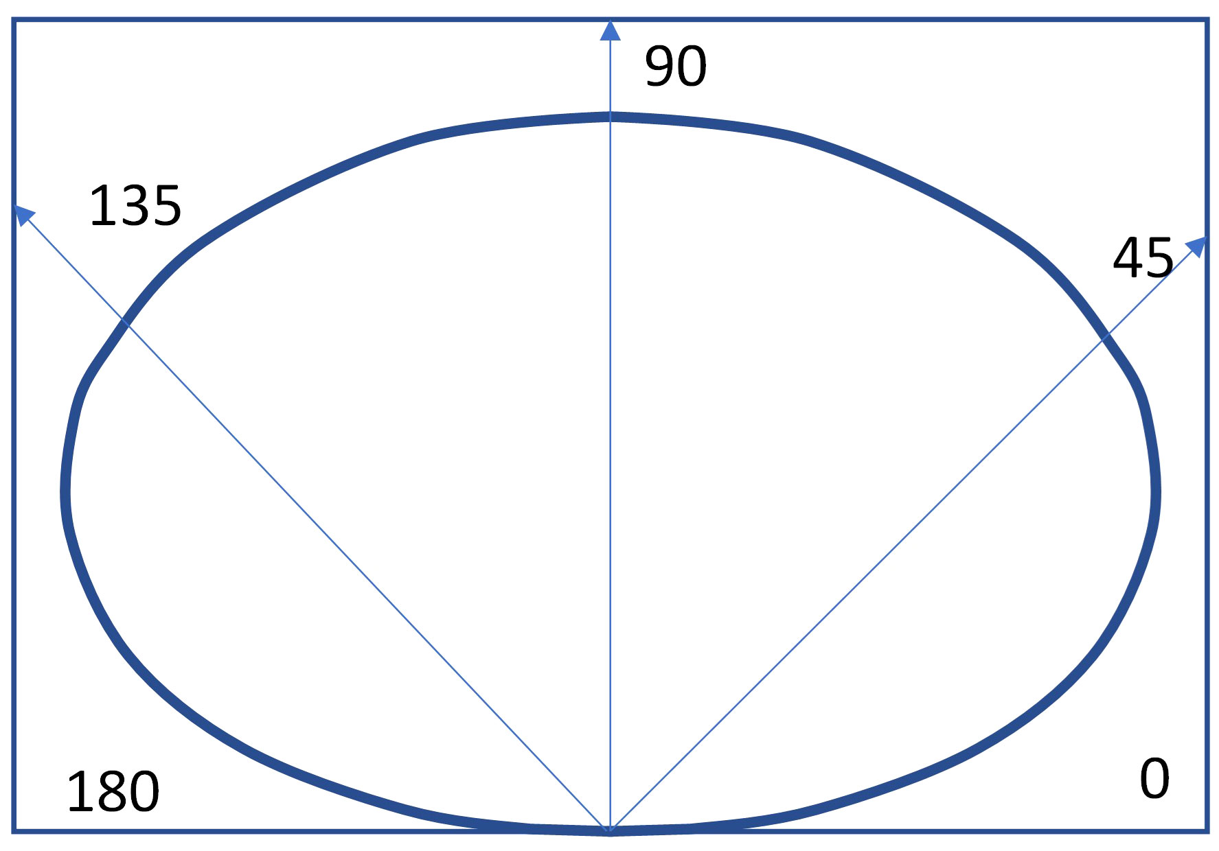
Figure 4 A “mushroom-like” antenna pattern in elevation and circular in azimuth.

2.2 Loss mechanisms

According to (Yang et al)., the REL model includes the following propagation mechanisms between a LEO satellite and a sea surface object, such as a buoy:

● The reflection and scattering from specular points on a moving sea surface (from (Yang et al.)).

● Shadowing caused by steep sea waves that block radio waves to be reflected from the sea surface to the antenna (see (B. J. Smith, 1967)).

● The “spreading” of reflections from the curved earth surface is caused by the divergence effect. Because of the long distance to the satellite, this effect is insignificant in our case and is ignored.

● Diffraction caused by the round earth when the satellite is below the horizon or at low elevation angles.

● Free space and atmospheric loss mechanisms when the radio wave propagates to/from the buoy.

2.2.1 Scattering from the sea surface

The reflection from the rough sea surface is represented as an effective reflection coefficient R_rough. According to the Kirchhoff theory (Molish, 2006), R_rough is given by the expression:

$\begin{array}{ll}\begin{array}{c}{\mathit{\text{R}}}_{\mathit{\text{rough}}}=\mathit{\text{R}}·\mathit{\text{exp}}\left[-\mathbf{2}{\left\{\frac{\mathbf{2}\mathit{\text{π}}{\mathit{\text{σ}}}_{\mathit{\text{h}}}\mathit{\text{sin}}\mathit{\text{γ}}}{\mathit{\text{λ}}}\right\}}^{\mathbf{2}}\right]\end{array}& (8)\end{array}$

The variables in the above equation are defined in Table 1. A varying EM field at the antenna superimposed on this average will contribute to fading and is part of the fading statistics.

From Figure 5, it is seen that for a rough sea, the reflection from the sea vanishes from a certain value of the elevation angle. This is depending on the roughness of the sea.

FIGURE 5

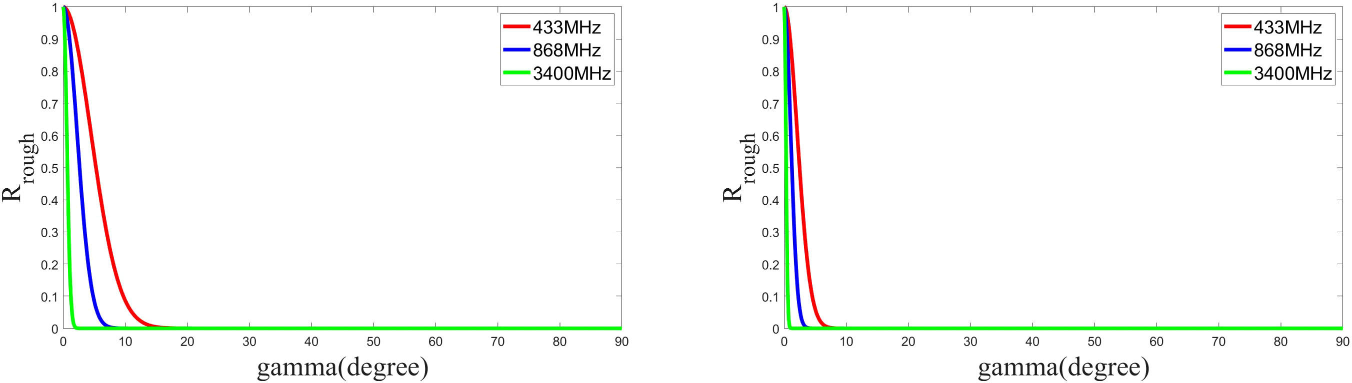
Figure 5 The reflection coefficient R_rough at frequencies 433, 868, and 3,400 MHz. rms height and slope of sea waves: to the left, 0.7 m and rms slope of 0.1 m/m, and to the right, 1.5 m and rms slope of 0.2 m/m.

2.2.2 Shadowing by sea waves

According to (Yang et al)., shadowing is caused by sea waves where the incident ray has an elevation angle that will shadow reflection or scattering points from the sea surface. The reflection from the sea surface will always be reduced by this effect. Smith (1967) proposed a shadowing coefficient, which can be written as

$\begin{array}{ll}\begin{array}{c}{\mathit{\text{S}}}_{\mathit{\text{fun}}}=\frac{\mathbf{1}-\mathbf{0.5}\mathit{\text{erfc}}\left(\frac{\mathbf{\text{cot}}{\mathit{\text{θ}}}_{\mathit{\text{i}}}}{\sqrt{\mathbf{2}}{\mathit{\text{β}}}_{\mathbf{0}}}\right)}{\mathit{\text{Λ}}\left(\mathbf{\text{cot}}{\mathit{\text{θ}}}_{\mathit{\text{i}}}\right)+\mathbf{1}}\end{array}& (9)\end{array}$

Here, erfc is the complementary error function, and

$\begin{array}{ll}\begin{array}{c}\mathit{\text{Λ}}\left(\mathbf{\text{cot}}{\mathit{\text{θ}}}_{\mathit{\text{i}}}\right)=\frac{\mathbf{1}}{\mathbf{2}}\left(\sqrt{\frac{\mathbf{2}}{\mathit{\text{π}}}} \frac{{\mathit{\text{β}}}_0}{\mathbf{\text{cot}}{\mathit{\text{θ}}}_{\mathit{\text{i}}}}\mathit{\text{exp}}\left[-{\left(\frac{\mathit{\text{cot}}{\mathit{\text{θ}}}_{\mathit{\text{i}}}}{\sqrt{\mathbf{2}{\mathit{\text{β}}}_0}}\right)}^{\mathbf{2}}\right]-\mathit{\text{erfc}}\left(\frac{\mathit{\text{cot}}{\mathit{\text{θ}}}_{\mathit{\text{i}}}}{\sqrt{2{\mathit{\text{β}}}_0}}\right)\right)\end{array}& (10)\end{array}$

The other variables are defined in Table 1.

From Figure 6, it is seen that the shadowing has no impact when the elevation angle is above 25°–30° in rough sea, and ≈15° in moderate sea roughness.

FIGURE 6

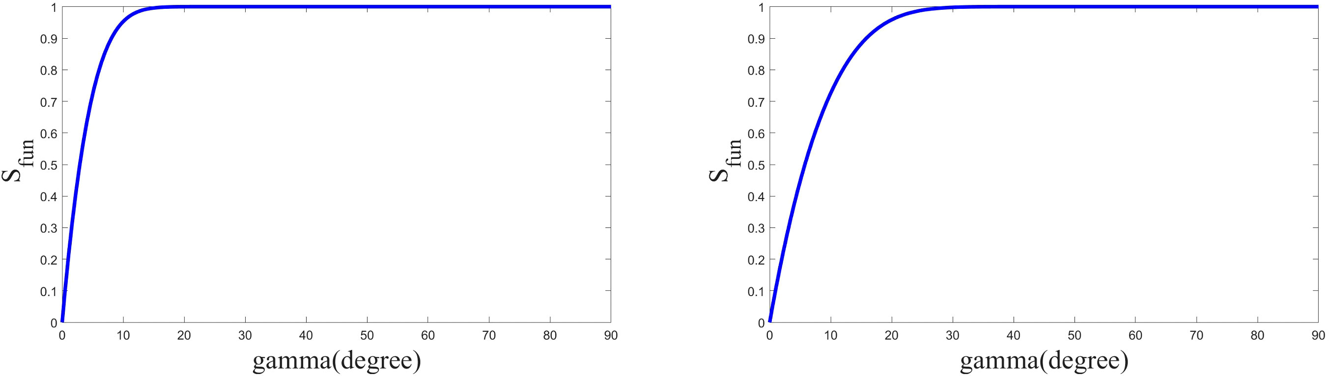
Figure 6 The shadowing coefficient S_fun. rms height and slope of sea waves: To the left, 0.7 m and rms slope of 0.1 m/m, and to the right, 1.5 m and rms slope of 0.2 m/m.

2.2.3 Diffraction loss

The diffraction loss is an additional loss to the free space loss. Figure 7 depicts four scenarios for the satellite’s position relative to the buoy. The diffraction loss is determined by these four scenarios and will be discussed further below.

FIGURE 7

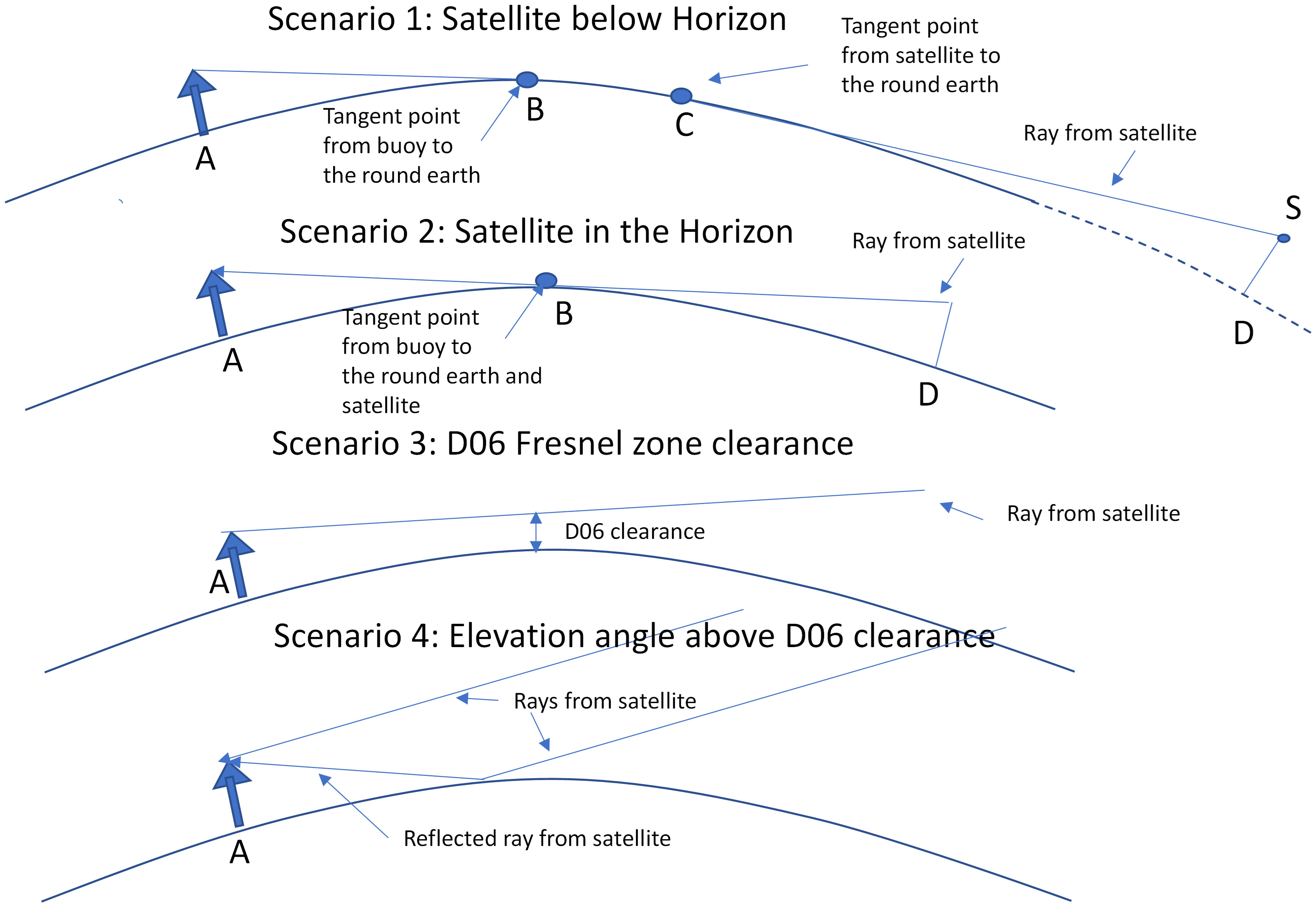
Figure 7 Four scenarios for satellite positions with respect to the buoy. The size of the buoy is blown up for illustration purposes, and the earth curvature and other dimensions are not aligned.

Scenario 1:

In this scenario, the satellite is below the horizon relative to the buoy. The length of the arc along the buoy (at point A) to the earth’s tangent point (at point B) is denoted by d₁. The length of the arc along the earth’s surface between tangent points B and C is d₃. The length from tangent point C to the satellite’s zenith point D at point S is d₂. In this case, there will be diffraction loss, which increases significantly when the satellite is beyond the horizon as seen from the buoy at point A.

Scenario 2:

In this scenario, the satellite is in the horizon with respect to the buoy. The length d3 = 0 in this case. There will be a diffraction loss in this case due to the interaction of radio waves with the earth’s surface.

Scenario 3:

In this scenario, the direct ray from the satellite has a clearance over the earth’s surface, which corresponds to a clearance of 0.6 of the First Fresnel Zone (FFZ) (Rappaport, 2002). In this case, the diffraction loss is zero. This corresponds to the D06 distance between the satellite and the buoy.

Scenario 4:

In this scenario, the direct ray from the satellite has an elevation angle with no diffraction. D_LOS is the distance between the satellite and the buoy.

Diffraction enables radio transmission even below the line of sight. However, this comes at the expense of diffraction loss. (Norton, 1941; Bullington, 1947; ITU-R Recommendation P.526-13, 2013) describe the diffraction theory of ground-wave propagation over a smooth spherical earth, which can be applied to open sea geometry. According to (Yang et al). the radio link’s total arc distance d is divided into three arc distances d₁, d₂, and d₃. Each of these distances are associated with losses L₁, L₂, and L₃, respectively. Referring to the scenarios in Figure 7, the distance d is the arc length between points A and D, distance d₁ is between A and B, distance d₂ is between C and D, and distance d₃ is between B and C.

Depending on the scenarios described above, the losses L₁, L₂, and L₃ can be calculated using the expressions in (Yang et al.) from Bullington’s paper (Bullington, 1947). The expressions are complex, and it is referred to (Yang et al).; (Bullington, 1947) for details and explanation of Equation 13. The diffraction loss L_dif for the different scenarios is given by the expression:

$$\begin{array}{c}{\mathit{\text{L}}}_{\mathit{\text{dif}}}={\mathit{\text{L}}}_{\mathbf{1}}+{\mathit{\text{L}}}_{\mathbf{2}}+\left|{\mathit{\text{L}}}_{\mathbf{3}}\right| \mathit{\text{if}} \mathit{\text{d}}\ge {\mathit{\text{d}}}_{\mathbf{1}}+{\mathit{\text{d}}}_{\mathbf{2}}\end{array}$$

$\begin{array}{ll}\begin{array}{c}{\mathit{\text{L}}}_{\mathit{\text{dif}}}={\mathit{\text{L}}}_{\mathbf{1}}+{\mathit{\text{L}}}_{\mathbf{2}}-\left|{\mathit{\text{L}}}_{\mathbf{3}}\right| \mathit{\text{if}} {\mathit{\text{D}}}_{\mathbf{06}}<\mathit{\text{d}}<{\mathit{\text{d}}}_{\mathbf{1}}+{\mathit{\text{d}}}_{\mathbf{2}}\end{array}& (13)\end{array}$

$$\begin{array}{c}{\mathit{\text{L}}}_{\mathit{\text{dif}}}=\mathbf{0} \mathit{\text{if}} \mathit{\text{d}}<{\mathit{\text{D}}}_{\mathbf{06}}\end{array}$$

The satellite case differs from the Bullington case because most of the path from the satellite to the buoy is above the troposphere, and we assume the impact of refraction to be insignificant.

2.2.4 Loss TX to RX including free space loss, diffraction, shadowing, and reflection

Using the results from previous sections, we can now define the losses that include the following effects:

● TX to RX distance,

● diffraction loss,

● mean loss caused by scattering from the sea surface to the buoy.

The composite loss, which comprises the TX/RX distance, shadowing and reflection from the rough sea, and diffraction, is given by:

$\begin{array}{ll}\begin{array}{c}{\mathit{\text{P}}}_{\mathit{\text{loss}}}=\mathbf{20}\mathit{\text{log}}\left\{\frac{\mathit{\text{λ}}}{\mathbf{4}\mathit{\text{π}}{\mathit{\text{D}}}_{\mathit{\text{LOS}}}}\right\}+\mathbf{20}\mathit{\text{lo}}{\mathit{\text{g}}}_{\mathbf{10}}\left(\mathit{\text{η}}\right)+{\mathit{\text{L}}}_{\mathit{\text{dif}}}\end{array}& (14)\end{array}$

where

$\begin{array}{ll}\begin{array}{c}\mathit{\text{η}}=\left|\mathbf{1}+{\mathit{\text{S}}}_{\mathit{\text{fun}}}·{\mathit{\text{R}}}_{\mathit{\text{rough}}}·\mathit{\text{exp}}\left(\mathit{\text{jk}}{\mathit{\text{Δ}}}_{\mathit{\text{d}}}\right)\right|\end{array}& (15)\end{array}$

When there is no reflection from the sea, the variable η equals 1. The wave number is represented by the parameter k. Table 2 shows the parameters used in the analysis.

TABLE 2

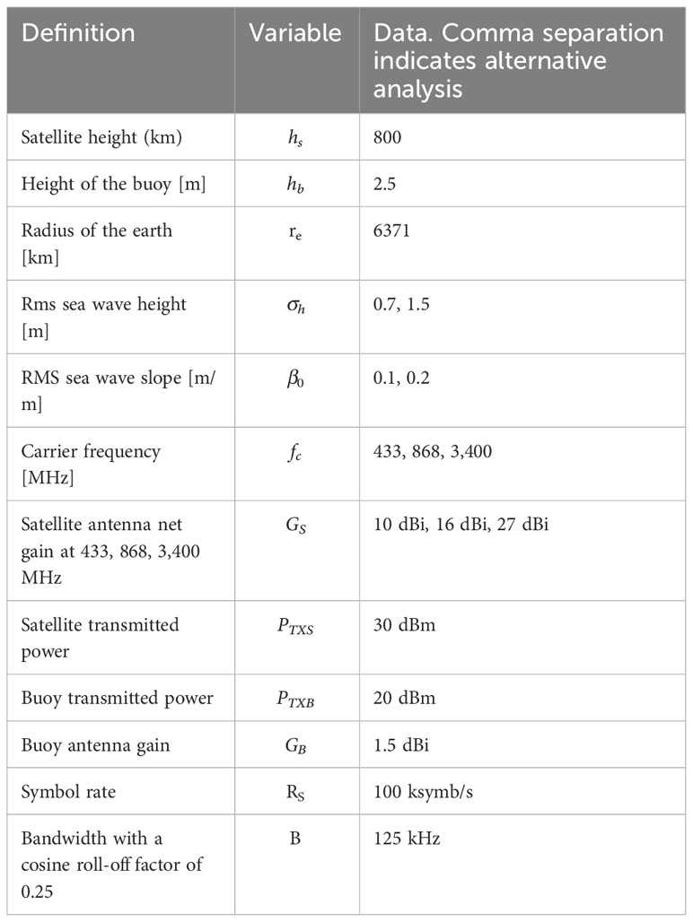
Table 2 Parameters used in the analysis.

Figure 8 shows that received signal level follows the free space loss down to an elevation angle where the impact of diffraction loss starts. This is at an elevation angle of a clearance of 0.6 to the First Fresnel Zone of the incoming radio waves to the buoy. This distance is denoted D06 and is shown on the figure. The “oscillations” of the curves to the left of the D06 distance is caused by reflections that occur at low elevation angle. The elevation angle at D06 is ≈1.4°. The reflections are moderate but visible on the curves due to the rough sea. It needs to be pointed out that the amplitude of the “oscillations” is larger in the left subfigure than in the right subfigure of Figure 8. The sea surface is calmer in the left figure case (rms height=0.7 m, rms slope=0.1 m/m) compared to the right case (rms height=1.5 m, rms slope=0.2 m/m). The steep part of the curves beyond D06 show that the diffraction loss is significant when the elevation angle is lower than the elevation angle corresponding to the distance D06. When the elevation angle becomes negative, it means that the satellite is below the horizon. This will be discussed further in the link budget analysis in Section 4. The radio waves will be subject to refraction in the relatively short part of the radio path crossing the troposphere. This will cause a small deviation of the elevation angle of the incoming radio wave compared to the case of no refraction. However, this impact has been disregarded in our analyses partly because it is complex and partly not significant and unimportant for the main discussions and conclusions.

FIGURE 8

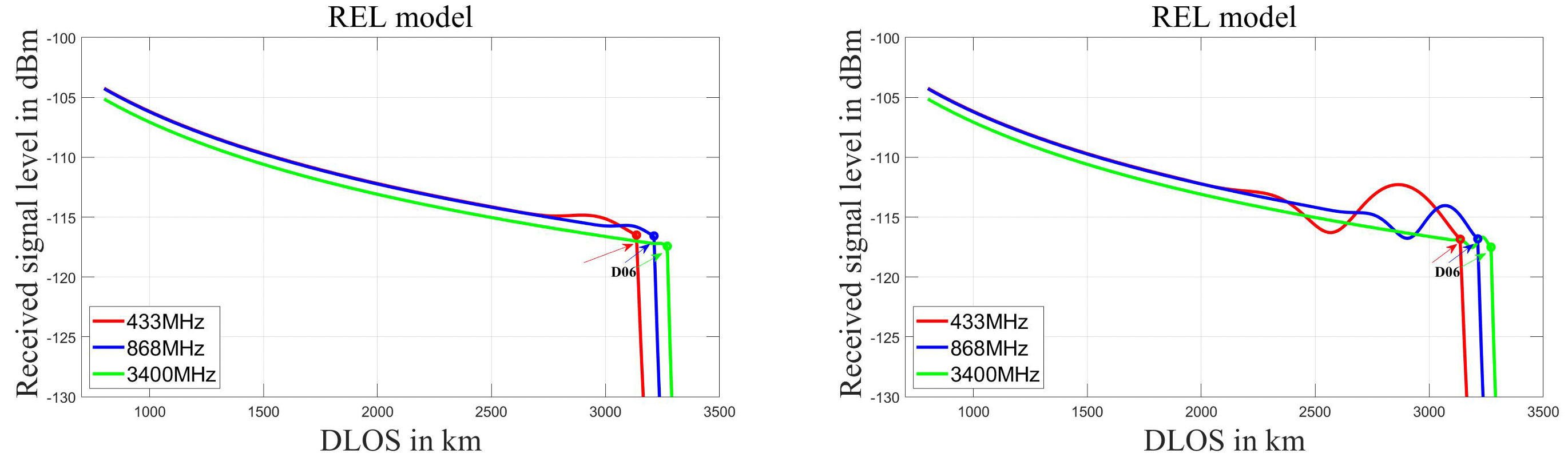
Figure 8 Received signal level in dBm with the distance D_LOS from the satellite to buoy at 433, 868, and 3,400 MHz, in which the EIRP from the satellite is 40 dBm at 433 MHz, 46 dBm at 868 MHz, and 57 dBm at 3,400 MHz, respectively. The loss includes free space loss, scattering/reflections from the sea, shadowing by sea waves, and diffraction loss. rms height and slope of sea waves: to the left, 0.7 m and rms slope of 0.1 m/m, and to the right, 1.5 m and rms slope of 0.2 m/m.

3 Atmospheric loss

3.1 Ionospheric propagation effects

We refer to the ITU documents in Telecommunication Union Radiocommunication Sector (ITU-R) P.1239-2 (2009). From Telecommunication Union Radiocommunication Sector (ITU-R) P.1239-2 (2009), the ionospheric propagation effects are the following:

● rotation of the polarization angle (Faraday rotation)

● group delay distortion

● scintillations

● change in direction of arrival due to refraction in the ionosphere. This is depending on the angle of incidence

● Doppler effect due to changes in electron density in the ionosphere over time

We do not include polarization rotation as we assume circular polarization. Furthermore, the group delay distortion will not be significant for the bandwidths (<1 MHz) considered for the IoT applications. We here refer to Figure 5 in the ITU-R P.531 document. When it comes to change in the direction of arrival due to refraction in the atmosphere, we recall some points from Telecommunication Union Radiocommunication Sector (ITU-R) P.1239-2 (2009). For low frequencies, in the VHF, as the frequency decreases, the atmosphere cannot be penetrated, or on the other side, a radio wave from a terminal will be reflected and cannot reach the satellite. Since the ionosphere is very variable in structure and density, the frequency at which these phenomena will occur is also variable and will depend on the path geometry. The frequency at which this may occur is changing with place on earth, diurnally and monthly. An estimate for this frequency is found in ITU recommendations ITU-R P.844 (Telecommunication Union Radiocommunication Sector (ITU-R) P.1239-2, 2009) and ITU-R P.1239 (Recommendation ITU-R P.1239-2, 2009. We assume here that the lowest frequency band considered, 433 MHz, is not affected by the non-penetrating phenomena. Furthermore, ITU-R P.531-14 also mentions ducting when the propagation is close to tangential to the ionosphere. The same document also mentions the Doppler effect due to fluctuations in the ionosphere. We discard the effect of Doppler or Doppler change rate caused by the ionosphere, as we assume this to be small compared to Doppler shift by other causes, e.g., movement of the satellite and the movement of the buoy on the sea surface.

Definition of some important effects and parameters in ITU-R P.531 describing the ionosphere are given below:

Electron density: n_e (el/m₃). Number of electrons per m³.

Total electron content (TEC) N_T, s is the variable distance along the radio path

$$N_T=\underset{s}{\int }{n}_e(s)ds$$

Scintillation index

$$S_4={\left(\frac{E(I^2)-{(E(I))}^2}{{(E(I))}^2}\right)}^{1/2}$$

Here, E denotes averaging and I the intensity of the signal (proportional to the square of the signal amplitude).

Nakagami density function p(I)

$$p(I)=\frac{2m^m}{\text{Γ}(m)}{I}^{m-1/2}\text{exp}(-mI)$$

The average intensity level of I is normalized to be 1.0 in the above expression.

The TEC changes with time due to the orbiting of the satellite. The TEC change in rate is contributing to the non-stationary nature of scintillation stochastic processes.

Hereafter, we focus on scintillation effects for the frequency bands of 433, 868, and 3,400 MHz and LEO satellites in orbits at height 800 km. We use the ITU-R P.531 document as a basis to assess and estimate scintillation effects and their impact on the propagation and, hence, the impact on the link budget. Furthermore, we focus on the scintillation effects that are valid for the Arctic Ocean, i.e., above the latitude of approximately 60°.

Scintillations are created by time fluctuations of the refractive index, which are caused by inhomogeneities in the medium. This will cause temporal fluctuations of the received radio signal with respect to:

● Amplitude

● Phase

● Direction of arrival changes

Scintillations is a stochastic process that is non-stationary in time and inhomogeneous in space. There are spatial fluctuations, and with the moving satellite, the short-time temporal behavior is also caused by this movement. This process is difficult to characterize, as it is depending on the following:

● an 11-year cycle with solar sunspot intensity (solar maximum and minimum)

● seasonal variations over the year

● time of the day (diurnal)

● geographical locations and geomagnetic activity

● frequency dependence

3.1.1 Instantaneous statistics

The scintillations may be described as a series of ionospheric scintillation events. During one such event, it may be meaningful to define a short-time statistic. A common parameter used to characterize the intensity of the fluctuation within an event is the scintillation index S₄ defined above. The scintillation is described as a variation in the received signal intensity I, where I is proportional to the square of the signal amplitude and may be regarded as a non-stationary stochastic process where the statistical parameters are changed with time. Measurements from Kiruna shown in the ITU-R P.531 document indicates that the averaging to estimate S₄ is over a time window in the order of 1 min. From these measurements, it is seen that the process is close to stationary within that time window.

During a scintillation event, the Nakagami distribution is accepted as an adequate description of the intensity distribution for a range of S₄ values. It is of interest to estimate the peak-to-peak fluctuations. Empirically, according to ITU-R P.531, a relationship between S₄ and the peak-to-peak fluctuations P_fluc(dB) is established:

$\begin{array}{ll}\begin{array}{c}{\mathit{\text{P}}}_{\mathit{\text{fluc}}}\left(\mathit{\text{p}}-\mathit{\text{p}}\right)=\mathbf{27.5}·{\mathit{\text{S}}}_{\mathbf{4}}^{\mathbf{1.26}}\left(\mathit{\text{dB}}\right)\end{array}& (16)\end{array}$

where 0<=S₄<=1

The scintillation is characterized as weak for 0< S₄<0.3, moderate for 0.3< S₄<0.6, and strong when 0.6< S₄<1. As S4 approaches 1, the intensity follows a Rayleigh distribution.

The temporal behavior, given an event, may be characterized by the autocorrelation function. A Fourier transform in ITU-R P.531 indicates that the peak spectrum is at 0.1–1 Hz, indicating a coherence time of 1–10 s of the scintillation intensity stochastic process.

3.1.2 Frequency dependence

For weak and moderate regimes of S₄, the frequency dependence is modeled as f^−ν, where ν=1.5 for most observations. Using this law with the lowest frequency, 433 MHz as reference, the scintillation index at frequencies 868 and 3,400 MHz is expected to be 0.35 and 0.13 times that of the 433 MHz case, respectively.

3.1.3 Seasonal and regional variations

The ionospheric scintillations have large regional and seasonal variations. It is referred to Figure 7 in ITU-R P.531. In the Arctic region, there is an intense zone at high latitudes with a fading depth of 5 dB in years of solar maximum. At years of solar minimum, it is far less. A typical scintillation event occurs at local ionospheric sunset and may last from 30 min to hours.

3.1.4 Angle of incidence

In most models, S²₄ is proportional to the secant of the zenith angle (or angle of incidence)

$\begin{array}{ll}\begin{array}{c}{\mathit{\text{S}}}_{\mathbf{4}}^{\mathbf{2}}=\mathit{\text{k}}\frac{\mathbf{1}}{\mathit{\text{cos}}{\mathit{\text{θ}}}_{\mathit{\text{i}}}}=\mathit{\text{k}}·\mathbf{\text{sec}}\left({\mathit{\text{θ}}}_{\mathit{\text{i}}}\right)\end{array}& (17)\end{array}$

The constant k is a proportionality constant. This model is believed to be valid up to θ_i close to 70 degrees.

3.2 IoT communications requirements

The requirements must consider the intermittent nature of the IoT data transfer. The requirements with respect to availability, latency, and interrupts of such communication is different from the continuous types of communications like, e.g., satellite broadcast and high-capacity terrestrial internet communications with fiber optics or radio relay systems.

In the ITU-R P.531 document, measurements, statistics, and empirics are presented. In our case with IoT to a buoy in the Arctic Ocean, the service is of the intermittent type, and we may afford to wait for a communication to take place if conditions are bad. This will have an impact on the link margin with respect to, e.g., scintillation that we must specify.

3.3 Assessing link margin for scintillations

When assessing the link margin that should be used for the scintillation effect, it is worthwhile to cite a paragraph in the ITU-R 531 document:

Due to the complex nature of ionospheric physics, system parameters affected by ionospheric effects as noted above cannot always be succinctly summarized in simple analytic formulae. Relevant data edited in terms of tables and/or graphs, supplemented with further descriptive or qualifying statements, are for all practical purposes the best way to present the effects.

From (Allnutt, 2011) (Allnutt), we recall the following: “The concept of annual statistics is of dubious merit for ionospheric phenomena.”

The above citation indicates that there is no straight-forward way to estimate a link margin for a specific application. We present an example to illuminate the situation with IoT communications from a satellite to a sensor on the sea surface. A satellite at a height of 800 km gathering IoT data from a region has a round earth trip time of 101 min. The satellite (if the orbit is at zenith with respect to the buoy) is then visible to a buoy approximately 15 min. Of these,<15 min is adequate for transmission due to increased path loss, diffraction loss, and increased scintillation with angle of incidence higher than 70° (elevation angle <20°). If a serious event of scintillation occurs within this time span, the communication may fail. The next possibility is the next passage of the satellite. In our case, the availability is depending on the probability of a serious event of scintillation during a passage. If we can allow to wait N passages for a successful transfer, the probability of a satisfactory transfer is the probability of not having N consecutive transfer failures. As we see, the availability in the situation of intermittent data transfer is depending on the following:

● The link budget margin in dB allowed for scintillation. Because there are power restrictions both in the LEO satellite and the data unit, e.g., a buoy, this margin cannot be too conservative (high value in dB). This margin is denoted M_s (dB).

● The number of successive passages allowed to wait for a successful transfer of data.

When setting the margin value, we must utilize all a priori information combined with known statistics. Furthermore, we evaluate the probability of scintillation depth not exceeding the margin M_s when one or more satellite passages are allowed.

We have chosen the following strategy:

● The lifetime of a LEO satellite is in the order of 3 years. The period between a solar maximum and minimum is 11 years. The scintillation depth, according to Figure 7 in (ITU-R P.531-14, 2019)," and latitude of 64°, there is a time span in the order of 3 h where the scintillation depth is 2 dB at 1.5 GHz and solar maximum and<1 dB at solar minimum. We choose 1.5 dB as a compromise value of scintillation depth at 1.5 GHz and use Equation 18 to estimate S₄ at the three frequencies of 433, 868, and 3,400.

● We compensate for the zenith angle using Equation 17. The margin against scintillation will define the maximum zenith angle for reliable data transfer. If the margin is critical, we may not have communications at high zenith angles (low elevation).

● When analyzing the probability of the scintillation intensity to be above the margin in dB set for scintillations, we assume that the scintillation intensity follows a Nakagami density distribution.

We use the frequency dependence f^−ν, where ν=1.5 to calculate S₄ at other frequencies. At an arbitrary frequency f, this will be

$\begin{array}{ll}\begin{array}{c}{\mathit{\text{S}}}_{\mathbf{4}}\left(\mathit{\text{f}}\right)={\left(\frac{{\mathit{\text{f}}}_{\mathit{\text{r}}}}{\mathit{\text{f}}}\right)}^{\frac{\mathbf{3}}{\mathbf{2}}}·{\mathit{\text{S}}}_4\left({\mathit{\text{f}}}_{\mathit{\text{r}}}\right)\end{array}& (18)\end{array}$

Here, f_r is the reference frequency, which is 1.5 GHz in the ITU-R document. Table 3 shows the S4 values for the frequencies considered. The scintillations at 433 MHz are in the “medium” category.

TABLE 3

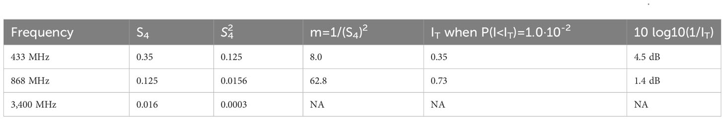
Table 3 Conversion of S4 from 1.5 GHz to the frequencies 433, 868, and 3,400 MHz, and the lower thresholds I_T where P(I<I_1T) = 10⁻².

At 45°, the correction factor of S₄ for the elevation angle is 1.2, and at 70°, as high as 1.7.

The Nakagami probability density function is given by:

$\begin{array}{ll}\begin{array}{c}\mathit{\text{p}}\left(\mathit{\text{I}};\mathit{\text{m}},\mathit{\text{Ω}}\right)=\frac{\mathbf{2}{\mathit{\text{m}}}^{\mathit{m}}}{\mathit{\text{Γ}}(\mathit{\text{m}})·{\mathit{\Omega }}^{\mathit{\text{m}}}}·{\mathit{\text{I}}}^{\mathit{\text{m}}-\frac{\mathbf{1}}{\mathbf{2}}}·\mathit{\text{exp}}\left(\frac{\mathit{\text{m}}}{\mathit{\Omega }}\mathit{\text{I}}\right),\forall \mathit{\text{I}}>0\end{array}& (19)\end{array}$

The cumulative Nakagami distribution P(I) of the intensity I is given by:

$\begin{array}{ll}\mathit{\text{P}}(\mathit{\text{I}})={\displaystyle \underset{\mathbf{0}}{\overset{\mathit{\text{I}}}{\int }}\mathit{\text{p}}(\mathit{\text{x}})\mathit{\text{dx}}}=\mathit{\text{Γ}}(\mathit{\text{m}},\mathit{\text{Im}})& (20)\end{array}$

where Γ(m,Im) is the incomplete Gamma function. In both expressions the functions are normalized, so the mean of the signal intensity E[I]= Ω=1. Furthermore, the parameter m is the inverse of the variance of the density function m=1/(S₄)². Hence, (S₄)² is the variance of the intensity I. This means that the peak-to-peak scintillation is low when m is high.

Figure 9 shows the Nakagami probability density function (PDF), to the left with m parameter corresponding to S₄ = 0.35 and to the right with m parameter corresponding to S₄ = 0.125. These S₄ parameters are shown in Table 3 for 433 MHz and 868 MHz, respectively. At 3.4 GHz, the parameter S₄ = 0.016 giving a very high m, and we can conclude that at 3.4 GHz, the scintillations are insignificant in our scenarios and is not assessed any further.

FIGURE 9

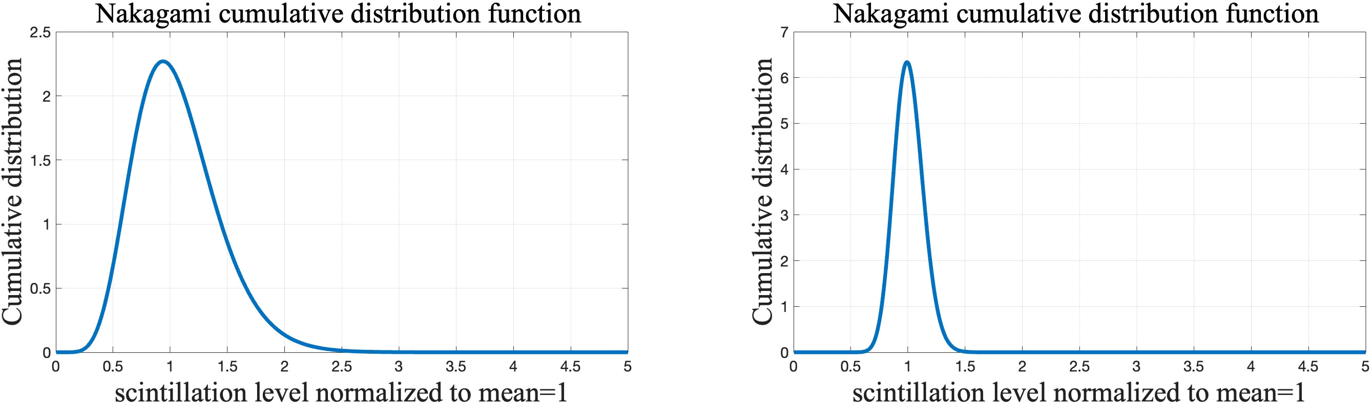
Figure 9 The Nakagami PDF. The left diagram is with S₄ = 0.35 (m=8), and the right is with S₄ = 0.125 (m=63).

The Nakagami PDF is shown in Figure 9. The left diagram is with S₄ = 0.35 (m=8), and the right is with S₄ = 0.125 (m=63). The threshold I_T is set at a level where P(I<I_T) = 1%. The probability P((I<I_T) is the area A₁ of the pdf that is below I_T. Figure 10 shows the lower tail of A₁. We set A₁ = 1%. The lower threshold is shown in Table 3, and the mean to I_T ratio in dB is also shown in the table.

FIGURE 10

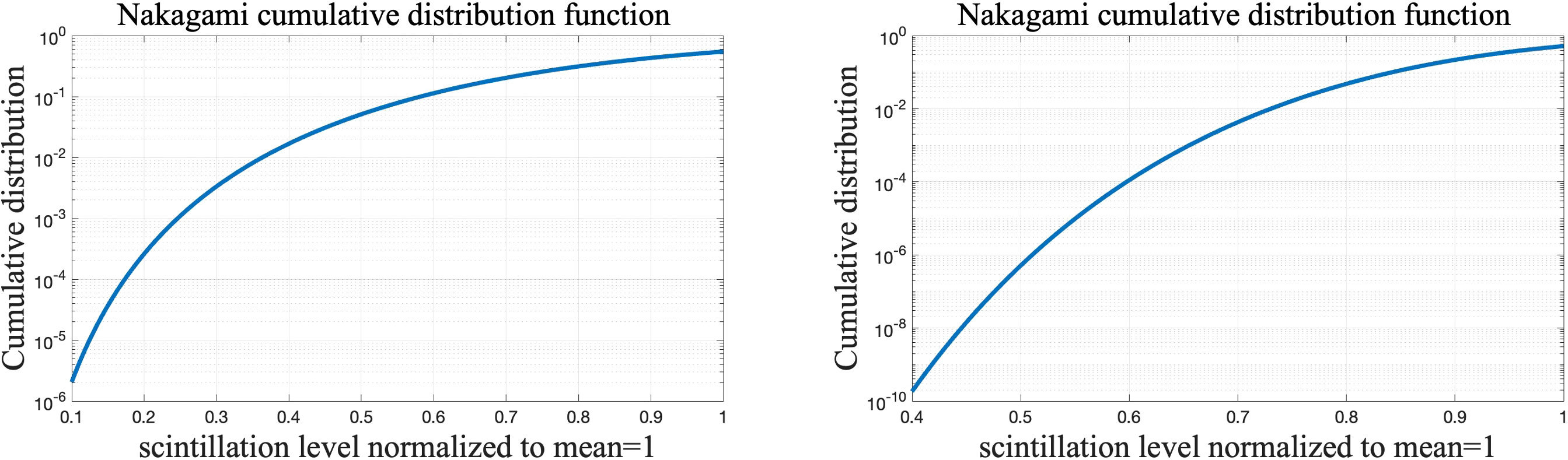
Figure 10 The Nakagami CDF. The left diagram is with S₄ = 0.35 (m=8), and the right is with S₄ = 0.125 (m=63).

The probability of the intensity depth I not exceeding 4.5 dB at 433 MHz and 1.4 dB at 868 dB is 1%. We can increase the availability by repeating the same message, either in the same satellite passage or in consecutive passages. We assume that the data transfer is organized as slots of data, each with error correction and of duration considerably shorter than the coherence time of scintillations and fading. It is possible to repeat the same data in the same passage n times with a time separation that is well above the coherence time of the scintillation stochastic process, i.e., >10 s. Then, the scintillations at all time instances of the N messages are statistically independent. The joint probability that all N messages experience a scintillation depth lower than I_T is (P(I<I_T))^N.

3.3.1 Discussion and conclusion on the setting of the link budget margin against scintillations

In the link budget, we set the scintillation margin to 4.5 dB and 1.4 dB at 433 MHz and 868 MHz, respectively. If this margin is too demanding, it is possible to wait sending messages until a quiet diurnal scintillation activity occurs. It is common for the radio system, e.g., DVB-RCS, to have physical level protocol that monitor the signal-to-noise ratio. If signal-to-noise ratio (SNR) is too low, retransmission of messages with the same content may be asked for. At 3,400 MHz, the scintillation is regarded as insignificant. However, there may be instances where scintillation may impact the communications also at this frequency. For comparison, we refer to Table 2 in (ITU-R P.618-13, 2017) with 1dB of probability<0.1% at “mid-latitude.” However, the conditions are not the same, and we use the above figures 4.5 dB and 1.4 dB in the following analysis.

3.4 Small-scale fading

The availability of measurements of small-scale fading caused by scattering from the sea surface is scarce. In the ICAO document ACP WG-F/31 oct 2014 (ICAO doc. ACP WG-F/31, 2014), and (DVB-RCS2 standard, 2014) propose to use rice fading with K≈30 dB and a delay spread in the order of 50 ns. According to the discussion in paragraph 2.2.4, fading due to scattering/shadowing occurs only at low elevation.

3.5 Tropospheric attenuation

3.5.1 Precipitation and clouds

An empirical method based on the knowledge of rain intensity and path elevation angle is elaborated in the ITU-R document (Telecommunication Union Radiocommunication Sector (ITU-R) P.1239-2, 2009). According to Telecommunication Union Radiocommunication Sector (ITU-R) P.1239-2 (2009); Recommendation ITU-R P.838-3, the attenuation due to precipitation in the Arctic Ocean at the frequencies of 433 MHz, 868 MHz, and 3,400 MHz is insignificant even for a slant elevation angle. In the link budget of Table 4, we have used 0.3 dB for 433 MHz and 868 MHz, and 0.5 dB for 3,400 MHz.

TABLE 4

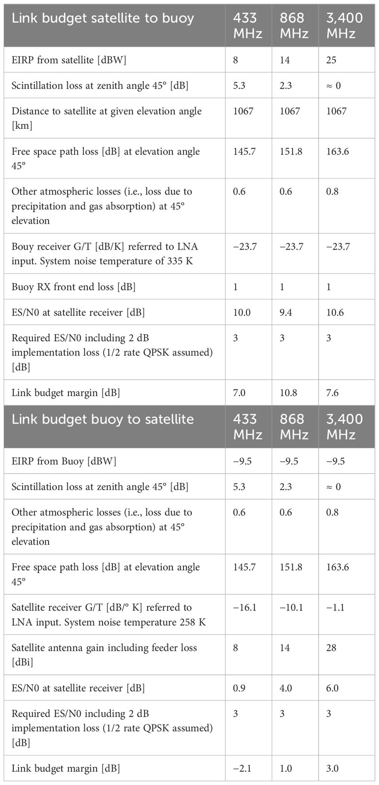
Table 4 Link budget for the radio link from buoy to satellite and satellite to buoy at the three frequencies of 433, 868, and 3,400 MHz.

3.5.2 Attenuation caused by gases

According to ITU-R P.618-13, Section 2.1, the attenuation caused by absorption in vapor and oxygen depends on frequency, vapor density, elevation angle, and height above sea level. In the book (Ippolito, 1986) by Ippolito, tables show that the attenuation at 1–4 GHz, 60% relative humidity, and 45° elevation angle is 0.3 dB. At 5° elevation angle, the attenuation is increasing to 2.2 dB. We have used a loss of 0.3 dB at elevation angle of 45° for the link budget in Table 4.

4 Link budget analysis

4.1 Impact of the buoy’s antenna

Mechanical antenna design is very demanding in the harsh weather conditions that are met in the Arctic Ocean. As the mechanical design and real antenna pattern design are outside the scope of this paper, we focus on the electrical parameters of an idealized antenna pattern. The antenna diagram must cover the hemisphere and have a “mushroom-like” antenna pattern. An example and an idealized pattern are shown in Figure 4.

As with the “mushroom-type” antenna pattern described above, the gain is low at low elevation angle. This may imply that we are not able to send or receive data below a critical elevation angle with a gain not able to close the link budget to/from the LEO satellite. Furthermore, the buoy will move with the sea waves. The angular movements are depending on the buoy’s mechanical design. A combination of elevation angle to the satellite, seen from the buoy, and the angular movement of the buoy will define the instantaneous gain at time τ. The instantaneous zenith angle of the buoy is ϕ(τ), and the elevation angle at the buoy’s position to the satellite is γ. The gain of the antenna in the direction of the satellite is then time varying and given by

$\begin{array}{ll}\begin{array}{c}\mathit{\text{G}}\left(\mathit{\text{γ}}+\mathit{\text{ϕ}}\left(\mathit{\text{τ}}\right),\mathit{\text{ψ}}\right)\end{array}& (21)\end{array}$

The angle ψ is the azimuth angle. The antenna is assumed omnidirectional in azimuth, and the antenna gain is independent of ψ. In harsh weather, MAX(ϕ(τ))≈20-25. It is obvious that we cannot design a system with maximum angular movement of the buoy. The communication of data to and from the satellite will be in bursts controlled by a TDMA system. The length of bursts can be from 10 to 50 ms. The maximum angular movement rate (rad/s) of the antenna is expected to be in the order of 10–20°/s. Hence, the angular movement within a burst will be<1–2°. If ϕ(τ) is close to worst case combined with low elevation angle, we must accept loss of a burst and must wait for a better ϕ(τ) or a better elevation angle γ. In the link budget analysis, we use G_MAX=2.5 dB and a minimum gain of 1.5 dB caused by either low γ or a bad ϕ(τ). We assume a circular polarized antenna to avoid the 3-dB loss of a linear polarized antenna. A feasible design of a circularly polarized hemispherical pattern helix antenna with >2.5 dB gain is shown in (Slade, 2015). In the link budget analysis, we have assumed the same gain for the frequencies 433, 868, and 3,400 MHz. This means that there are different antennas for the three frequencies.

4.2 Link budget

Table 4 shows the link budget from satellite to buoy and buoy to satellite for all three frequencies. The link budget is calculated using the parameters in Table 2. We assume the 1/2 rate QPSK modulation and coding scheme according to the DVB-RCS2 standard (2014). With a symbol rate of 100 ksymb/s, the data rate is 100 kbit/s. One carrier will then occupy a bandwidth of 125 kHz using a cosine roll-off factor of 0.25 in the pulse shaping filter. The elevation angle in the analysis is 45°, which means that there is no diffraction loss, and the impact of scattering/shadowing is not present at this angle. From the discussions in Section 3.5, we use 0.6 dB atmospheric loss at 433 MHz and 868 MHz, and 0.8 dB at 3,400 MHz. As expected, the link from the buoy to satellite is critical because of the low output power from the buoy. At 433 MHz, we have a 1.8-dB negative margin, which means that the scintillation depth cannot exceed 3.5 dB corresponding to a probability of P(I<I_T)=3%, using the left part of Figure 10. At 868 MHz and 3,400 MHz, the link budget has a margin. In the direction from satellite to buoy, the margin is good.

At low elevation angle, the communication from buoy to satellite is not possible due to increased path length and increased scintillation at slant radio paths.

5 Conclusion

When the elevation angle of the radio waves to a buoy on the sea surface is low, the scattering/shadowing from the sea surface will have an impact. The impact is decreasing with the roughness of the sea. The elevation angle where reflection has an impact on the loss is increasing with decreasing sea surface roughness. The diffraction loss is insignificant when the elevation angle corresponds to a distance equal to or shorter than D06. The distance D06 corresponds to the distance with clearance of 0.6 of the First Fresnel Zone of the incoming radio waves to the buoy. Beyond D06, the diffraction loss is increasing fast. Furthermore, with decreasing elevation angle, the scintillation depth will increase and reduce the probability of successful delivery of data from the buoy to the satellite.

The link budget is most demanding for the uplink, from the buoy to the satellite. The example parameters that we have used show that closing the link budget, even at an elevation angle of 45°, is difficult at the lowest frequency, 433 MHz, with an scintillation loss margin of 5.3 dB. IoT communication to and from a buoy to a single LEO satellite is of the intermittent type. A burst type of physical layer with bursts duration of 20–50 ms with a strong FEC code and a low-rate modulation scheme like 1/2 rate QPSK with interleaving will operate at a low ES/N0. If data cannot be detected, retransmission may be invoked to secure delivery. The gross data rate with the proposed MODCODE scheme is 100 kbit/s. In situations with changing conditions that are typical with satellite communication with a buoy on the sea surface in a harsh environment, it is obvious that the data capacity is limited.

The mechanical design of the buoy and antenna design are crucial. We believe that using an adaptive antenna presently is not feasible for stand-alone buoys in the open sea due to power restrictions. However, clever antenna design reducing the impact of antenna mismatch during the buoy’s movement on the sea surface is crucial. It is also essential to make a mechanical design with respect to inertial properties that are reducing the angular movement on the sea surface. These aspects have been outside the scope of this paper and may be subject to further research together with practical implementation and field tests.

Theoretically, communication is possible beyond the line of sight. However, this is unlikely because the link budget in the uplink is demanding, and the antenna movement combined with low gain at low elevation angle makes this even more demanding. The main radio parameters of a buoy floating on the open sea and a LEO satellite with moderate cost, as shown in the link budget of Table 4, is assumed to be state of the art of such systems. To make possible communications at low elevation (and hence, increased connection time per satellite passage), the main radio parameters (EIRP and G/T) of both the satellite and the buoy must be improved considerably.

Data availability statement

The raw data supporting the conclusions of this article will be made available by the authors, without undue reservation.

Author contributions

TR and KY contributed to the theoretical analysis while CW contributed to the simulation results. All authors contributed to the article and approved the submitted version.

Funding

This work was supported by Basic Scientific Research Fund of Zhejiang Provincial Universities under Grant No. 2021JD004.

Acknowledgments

Hao Zeng, the master student in Ocean Connectivity Lab of Zhejiang Ocean University, is highly appreciated for his effort doing part of the editing work.

Conflict of interest

The authors declare that the research was conducted in the absence of any commercial or financial relationships that could be construed as a potential conflict of interest.

Publisher’s note

All claims expressed in this article are solely those of the authors and do not necessarily represent those of their affiliated organizations, or those of the publisher, the editors and the reviewers. Any product that may be evaluated in this article, or claim that may be made by its manufacturer, is not guaranteed or endorsed by the publisher.

References

3GPP (2019). “Study on management and orchestration aspects of integrated satellite components in a 5G network,” in 3rd Generation Partnership Project (3GPP), Technical Report (TR) 28.808, 9 2019, version 0.2.0.

Google Scholar

Allnutt J. E. (2011). Satellite-to-Ground Radiowave Propagation. 2nd (London, United Kingdom: The Institution of Engineering and Technology).

Google Scholar

Birkeland R., Palma D. (2019) in An assessment of IoT via satellite: Technologies, Services and Possibilities. 70th International Astronautical Congress (IAC), Washington, USA: International Astronautical Congress, 21-25 October 2019.

Google Scholar

Smith B. J., (1967). “Geometrical Shadowing of a Random Rough Surface,” IEEE Transaction on antenna and propagation, VOL. AP-15, NO. 5.

Google Scholar

Bullington K. (1947). Radio propagation above 30 megacycles. Proc. IRE. doi: 10.1109/JRPROC.1947.232600

CrossRef Full Text | Google Scholar

DVB-RCS2 standard (2014). ETSI EN 301 545-2 V1.2.1.

Google Scholar

ICAO doc. ACP WG-F/31 (2014). L-Band and C-Band Air Ground Channel measurements & Modeling update.

Google Scholar

Ippolito L. J. Jr. (1986). Radiowave Propagation in Satellite Communications. 1st (Van Nostrand Reinhold Company Inc.).

Google Scholar

ITU-R Recommendation P.526-13 (2013). Propagation by diffraction.

Google Scholar

LoRaWAN® (2020). 2 1.0.4 Specification (TS001-1.0.4) (LoRa Alliance, Inc).

Google Scholar

Molish A. F. (2006). Wireless Communications (John Wiley & Sons, Ltd.).

Google Scholar

Norton K. A. (1941). The calculation of ground-wave field intensities over a finitely-conducting spherical earth. Proc. IRE. doi: 10.1109/JRPROC.1941.233636

CrossRef Full Text | Google Scholar

Palma D., Birkeland R. (2018). Enabling the internet of arctic things with freely-drifting small-satellite swarms. IEEE. doi: 10.1109/ACCESS.2018.2881088

CrossRef Full Text | Google Scholar

Rappaport T. S. (2002). Wireless Communications, Principles and Practice, Second Edition, Prentice Hall.

Google Scholar

Recommendation ITU-R P.1239-2 (2009). ITU-R reference ionospheric characteristic.

Google Scholar

Recommendation ITU-R P.838-3. (2005). Specific attenuation model for rain for use in prediction methods, Question ITU-R 201/3.

Google Scholar

RESOLUTION 248 (WRC-19) (2019). “Studies relating to spectrum needs and potential new allocations to the mobile satellite service in the frequency bands 1 695-1 710 MHz, 2 010-2 025 MHz, 3 300-3 315 MHz and 3 385-3 400 MHz for future development of narrowband mobile-satellite systems,” in The World Radiocommunication Conference, Sharm el-Sheikh.

Google Scholar

Slade B. (2015). The Basics of Quadrifilic Helix Antennas, Technical article, Orban Microwave Products.

Google Scholar

Telecommunication Union Radiocommunication Sector (ITU-R) P.1239-2. (2009). ITU-R reference ionospheric characteristic.

Google Scholar

Wei T., Feng W., Chen Y., Wang C.-X., Ge N., Lu J. (2020). Hybrid satellite-terrestrial communication networks for the maritime internet of things: key technologies, opportunities, and challenges. IEEE Internet Things J. 8 (11). doi: 10.1109/JIOT.2021.3056091

CrossRef Full Text | Google Scholar

Yang K., Molisch A. F., Ekman T., Røste T., Berbineau M. (2019). A deterministic round earth loss model and small-scale channel properties for open-sea radio propagation. IEEE Trans. Vehicle Technol. 68 (9). doi: 10.1109/TVT.2019.2929914

CrossRef Full Text | Google Scholar