Assessing marine heat waves in the Mediterranean Sea: a comparison of fixed and moving baseline methods

1 Introduction

Marine heat waves (MHW) are local, prolonged, anomalously warm sea temperature extreme events. Since the first formal statistical definition that allowed a systematic study of these extreme warm water events was put into use (Hobday et al., 2016), there has been increasing interest among the scientific community to scrutinize the reach, impact, and usefulness of this novel ocean indicator, both for scientific purposes and stakeholder engagement (Hobday et al., 2018). Numerous articles have been published about this emerging field, covering topics ranging from its most suitable definition, drivers, modelling, environmental and socioeconomic impact, and analysis of regional MHW statistics (Holbrook et al. (2020), and references therein).

Recent regional and global studies on MHW portray increasing trends in annual number of MHW days, intensity, and duration (Oliver et al., 2018; Jacox, 2019; Juza et al., 2022; Dayan et al., 2023). Such studies exploit reference baselines fixed in the past as a benchmark for the comparison of recent events, thus incorporating into their framework the long-term secular warming of the seas (Stocker et al., 2013) on top of short term SST variability. Secular warming thus turns out to be the main driver of MHWs globally (Oliver, 2019), and model-based projections based on these criteria predict a constant global scale MHW in the coming decades (Frölicher et al., 2018). Given the prospect of year-long MHW events under the current MHW definition consensus, there have been discussions as to whether the optimal choice of baseline periods should be fixed in the past or shifted in time (Holbrook et al., 2020), thus decoupling long-term warming from short-term variability. Recently, Amaya et al. (2023) advocated for using the term “marine heat waves” exclusively for events identified with a shifting baseline definition, emphasizing the distinction between transient extreme events and the ‘long-term temperature trends’ associated with gradual warming patterns.

This study investigates extreme sea surface temperature (SST) events in the Mediterranean Sea, with a focus on comparing Marine Heat Wave (MHW) statistics using both fixed and moving baseline periods for the analysis. We do so by first comparing projections of annual MHW days for daily satellite SST data and a set of Earth System Models (ESMs) from the Coupled Model Intercomparison Project Phase 6 (CMIP6) (Eyring et al., 2016). We then make a more detailed analysis of moving baseline historical MHW metrics for the Mediterranean Sea over the period 2002–2021.

2 Data and methodology

2.1 Satellite SST data

In this work, marine heat waves were detected from a daily (nighttime) sea surface temperature (SST) dataset of the Mediterranean Sea (SST_MED_SST_L4_REP_OBSERVATIONS_010_021¹) freely distributed by Copernicus Marine Environment Monitoring Service (CMEMS). The product consists of an optimally interpolated grid (0.05°×0.05°) of foundation SST estimates covering the period from 1982 to 2021 (Merchant et al., 2019).

Working with foundation SST estimates means that the detected MHWs will be representative of the top 10 meters of the water column and independent of diurnal fluctuations (Pisano et al., 2016), which may result in an additional warming of more than 5°C at the sub-skin layer (1 mm depth) during summer under clear sky conditions (Pisano et al., 2022). Although in this work we have not taken into consideration sub-skin diurnal fluctuations while studying MHW statistics over the Mediterranean Sea, they offer a relevant piece of additional information when studying single MHW events, especially during summer when fluctuations are higher in magnitude (see Supplementary Figure S1 for seasonal SST daytime-nighttime differences in the Mediterranean Sea).

The daily nighttime SST dataset is complemented by daily SST standard deviation error estimates arising from interpolation errors. These estimates are provided in the same CMEMS data product, and we used them to estimate the uncertainties in local annual MHW metrics. More specifically, we calculated the upper (lower) error bounds by applying the MHW definition to SST time series resulting from adding (subtracting) the respective daily interpolation error. On average, the error is more persistent during winter months when cloud cover is more prevalent, hindering the accurate measurement of SST through infrared radiation-based remote sensing methods, as clouds are opaque to infrared radiation (Donlon et al., 2012). The winter mean error value is 0.25 °C, while the error is at its lowest during summer months, with a mean error value of 0.09 °C (see Supplementary Figure S2). Accounting for the SST interpolation error can result in ambiguity when characterizing certain MHW events, as single long events may be split into shorter ones after the lower bound of the error has been considered. One example of these uncertainties in MHW event detection is shown in Supplementary Figure S3 for a grid-point location at the Eonian Sea.

2.2 CMIP6 SST data

We examined Mediterranean Sea SST outputs from CMIP6 (Eyring et al., 2016). All models contain a simulation of a historical period, covering 1850-2014; along with projected future climates (experiments), covering 2015-2100. The latter represent the evolution of the Earth’s climate system subject to different anthropogenic greenhouse gas emission scenarios linked to a specific shared socioeconomic pathway (SSP) (Kriegler et al., 2014). We calculate the annual count of MHW days only considering the most pessimistic and optimistic scenarios available: a low-emission scenario (SSP1–2.6) which assumes that anthropogenic ${\text{CO}}_2$ emissions show a rapid decline in the coming decades and then stabilize at a radiative forcing of 2.6 $\text{W}/{\text{m}}^2$; and high emission scenario (SSP5–8.5) which assumes that these emissions continue to rise throughout the 21st century with radiative forcing reaching $8.5\text{W}/{\text{m}}^2$ by 2100 (Riahi et al., 2017). We computed annual MHW statistics in the Mediterranean Sea for 2002–2100 for a total of 22 ESMs, which accounts for most of the currently available models containing daily SST time series for both the SSP1-2.6 and SSP5-8.5 scenarios (see Tables S2, S3 in Supplementary Material). When multiple model runs were available for a certain model, a maximum of five were selected. We calculated MHW metrics for each of these runs, and took the ensemble median as the representative value for that particular model.

2.2.1 Model and satellite SST output for the Mediterranean Sea

Yearly average SST time series averaged over the Mediterranean basin for the 22 CMIP6 model simulations for 1850 to 2100, as well as satellite SST data, are shown in Figure 1. By 2100, the predicted ensemble mean SST over the Mediterranean is 24.32°C for SSP5-8.5 and 21.11°C for SSP1.2-6. To put that in comparison, the observed mean SST over the 30-year period 1992-2021 was 20.16°C. However, the ensemble range of SST predictions by 2100 is of great proportion with respect to its median value; being 24.46°C the median and 20.92–26.36°C the range for SSP5-8.5, and 21.13°C the median and 18.57–22.93°C the range for SSP1-2.6.

FIGURE 1

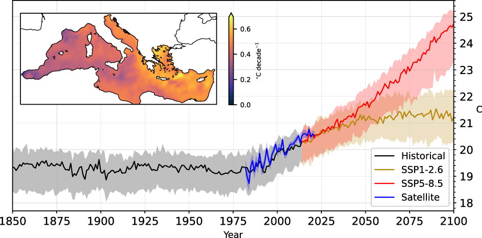
Figure 1 Annual SST for the Mediterranean Sea for CMIP6 models and satellite data, with an inset map of the Mediterranean Sea SST trend from satellite data. Solid black, yellow, and red lines correspond to the ensemble median SST of the 22 models used. Filled regions for Historical, SSP1-2.6, and SSP5-8.5 correspond to the model’s ensemble 70% confidence interval. The solid blue line corresponds to the mean SST from satellite SST data, with the filled blue region being the interpolation error from the SST dataset. Inset: Mediterranean Sea SST trend for the period 1982–2021.

The observed warming trend for the Mediterranean Sea as calculated from this study’s satellite SST dataset is 0.040°C/year (which is in agreement with a more detailed analysis made by Juza and Tintoré (2021)). In terms of the models’ output, the SSP5-8.5 shows accelerated warming in most simulations, with an ensemble average warming of 0.037 °C/year (0.012–0.055 °C/year ensemble range) for 2015 to 2050, and 0.058 °C/year (0.032–0.074 °C/year) for 2050 to 2100. In turn, SSP1-2.6 has a 0.022 °C/year (-0.001–0.046 °C/year) warming for 2015 to 2050 and shows a slight decline in warming in most models with a mean 0.003 °C/year trend (-0.009–0.020 °C/year) for 2050 to 2100. For more detailed information, refer to Tables S2, S3 in the Supplementary Material.

All models show a positive SST anomaly by 2100 (with respect to their 1982-2011 baseline), with 90% of SSP1-2.6 simulations showing a warming greater than 0.89°C, and 90% of SSP5-8.5 simulations showing warming greater than 3.76 °C. Satellite SST anomaly in 2021 with respect to the 1982-2011 baseline is 0.79°C.

3 Extreme events and marine heat wave definition

3.1 Definition of extreme event

There is no universal definition for extreme weather or climate events for any specific climate variable (Stephenson et al., 2008). The two main approaches to study climate extremes are based either on estimations of their probability of occurrence(e.g. by classifying a certain event as a 1-in-a-100 years event), or on the exceedance of a predefined threshold (Murray and Ebi, 2012). These thresholds for defining climate extremes mainly fall into two categories. 1. Absolute thresholds, usually defined by some value with well-known physical or societal implications (e.g. atmospheric temperature associated with certain health impacts.) 2. Statistical thresholds defined by values at the tails of a frequency distribution obtained from a predefined baseline reference period (with a time frame that may be days, months or years.) Statistical thresholds are commonly set to be the high (or low) percentile scores of the distribution, such as high 90th, 95th or 99th percentiles or the equivalent low 10th, 5th or 1st percentiles.

When assessing climate extremes, statistical thresholds have a major advantage over absolute thresholds (although they are not necessarily mutually exclusive in use) when analyzing the geographical and temporal extent of these events, as they are expressions of anomalies relative to the local climate and thus enable extreme events in different locations to be compared on an equal footing. On the other hand, absolute SST thresholds can be more suitable for marine science if defined by case-specific environmental metrics to assess ecological impacts. For example, an absolute threshold of roughly 28°C may be used to assess the thermal impact of posidonia oceanica meadows in the Balearic Sea (Marbà and Duarte, 2010).

Hobday et al. (2016) offered a MHW definition that has now become the standard among marine scientists. It is based on a seasonally varying statistical threshold set to be the 90th percentile of a local SST calendar-day probability distribution. Moreover, MHWs are defined to be prolonged in time, lasting for 5 or more days (neglecting 2-day or less gaps between events)².

3.2 Extreme events in a changing climate: fixed and moving reference baselines

In a stationary climate where frequency distributions of climate variables do not change in mean, scale, or shape, a statistical definition of extreme events would imply a fixed ‘rarity’ of such events, as thresholds are set to be exceeded at a fixed frequency (e.g. 10% for Hobday’s MHWs) during the reference period used to define the threshold (Klein Tank et al., 2009). However, this is not the case for many climate variables that are subject to long term climate variability, such as global surface temperature or SST, which on average show positive trends in the mean of their local distributions (Hansen et al., 2010; Stocker et al., 2013; Rey et al., 2020). These long-term changes, either in the mean, scale, or shape of the distributions, may lead to modifications of the probability of extreme events taking place. These changes are emphasized if we stick to a baseline period for threshold definition which is fixed in the past. This is because the old fixed baseline is no longer representative of current climate conditions, which may –but not necessarily– yield higher marginal probabilities above (or below) the threshold.

Regarding this issue, the World Meteorological Organization (WMO) officially resolved in 1956, while there was increasing knowledge of long term climatic fluctuations, that baseline periods should consist of the most recent 30-year periods in order to maximize the perceived relevance of those baselines to the community, which mainly should act as a benchmark for comparison of current observations (Trewin, 2007). The WMO still endorses this criteria to this day and defines climatological standard normals (baselines) to be consecutive 30-year periods which are to be updated each decade: 1 January 1981–31 December 2010, 1 January 1991– 31 December 2020, and so forth (Secretariat, 2019).

Using moving or transient baselines has been subject to debate (Soga and Gaston, 2018), as this practice is deemed to overshadow the impacts of a changing climate. However, there is still a crucial difference between choosing references periods for detecting long-term climate trends, and doing so to establish a benchmark against which current observations can be compared (WMO, 2012), the latter being the most relevant for studying climate extremes. In the case of detecting climate trends, it is common practice that in current climatological studies reference periods are chosen to be fixed in the past, especially during periods where anthropogenic influences are thought to be minimum. On the other hand, when evaluating climate extremes, which are essentially defined in terms of their probability of occurrence, relying on a fixed baseline can substantially alter the frequency of occurrence of such events to the point that it compromises the very definition of what an extreme event is. This last point will be further investigated for the case of MHWs in the Mediterranean Sea in the remainder of this article.

3.3 Marine heat waves and the warming ocean

The long-term global warming of the oceans (Stocker et al., 2013), and its more pronounced manifestation in the Mediterranean basin (reaching an SST trend of $0.038\pm 0.002\text{°C}/\text{year}$. over 1982–2020 (Juza and Tintoré, 2021), has been shown to be the main driver of long term MHW trends for most of the globe, including the Mediterranean (Oliver, 2019). This phenomenon has risen discussion about what the best criteria is for defining the range of the baseline period in order to set the threshold of MHWs. The discussion is currently whether it should be determined by a fixed baseline or a moving baseline, resolving that the choice should be context dependent and related to the environmental adaptation capabilities of the relevant ecosystems of the region under study (Holbrook et al., 2020). While the consensus is to use a period fixed at the beginning of the satellite era, it has been noted that sticking to this criteria would lead to world-wide MHW saturation in the coming decades, with annual MHW day-count eventually converging to a full year (Jacox, 2019). Moreover, saturation in MHW day-count per year semantically compromises the ‘wave’ aspect of an MHW, as the events will no longer be representative of perturbations of some property of the medium, but rather manifest a temperature offset with respect to some fixed period of the past (Jacox et al., 2020). Following analogous lines, similar incongruities arise when categorizing such events as “extreme”.

While the fixed baseline definition for MHW day-count saturation effectively communicates the message about Earth’s changing climate, it is important to consider its long-term applicability in identifying extreme events. In any case, evidence of climatic trends in SST related to anthropogenic climate change can be portrayed solely by means of annual SST anomalies, or, in relation to extreme temperatures, as trends in annual record-breaking SSTs over the whole satellite period.

We acknowledge the approach proposed by Amaya et al. (2023), which emphasizes the importance of differentiating between long-term temperature trends and marine heatwaves with a shifting baseline definition. According to their recommendations, ‘long-term temperature trends’ should be used to describe the slow changes in ocean temperature occurring over decades or longer, while the term ‘marine heatwave’ should be reserved for ocean temperature changes that are transient and extremely warm relative to the expected conditions for a given place and time, as defined by an evolving, recent climatological reference period. While we stand by this perspective, in the present article, we will use the term MHW to encompass both fixed and moving baselines to facilitate a comprehensive analysis of the topic.

To build a definition of a MHW that covers consistently rare extreme events, defined as local warm anomalies, we ought to incorporate the shift of the reference period in its definition. In this work we do so using a baseline period comprising the most recent 20-year period prior to the year under study. This involves, for example, using 2001–2020 as a reference for analyzing MHWs in the year 2021. We deviate from WMO recommendations in two ways. First, by setting the reference period to 20 years instead of 30. Although 30 years would be more desirable, we chose to stick to 20 years because, while avoiding the practice of using baselines whose range falls above the year under analysis, and as the satellite record starts in 1982, it allows us to compare MHW statistics in the Mediterranean Sea for a longer set of years (from 2002 to 2021), also incorporating the great 2003 MHW event into the statistics. In the context of a warming sea using longer moving baseline periods leads to an increase in the number detected MHW, as longer baselines contains “cooler” years that shift the threshold downward (see Supplementary Figure S4 for a comparison of detected MHW days using 20-year and 30-year baselines). Second, we use reference periods updated on a yearly basis instead of on a decadal basis. We chose this criteria because, as how we argued that statistical thresholds allow for MHW events to be compared equitably among different regions, updating the reference period yearly leads to a balanced intertemporal comparison between MHW events in much of the same way, with every event, regardless of the year, being representative of the same ‘rarity’ defined in the grounds of its most recent local climatology.

4 Results

In this work we extracted average MHW statistics for the Mediterranean Sea from a daily satellite SST time series, available for the period 1982–2021; and earth system model data from 22 CMIP6 simulations, which were trimmed to cover the period 1982–2100. We applied Hobday’s MHW definition, considering both a fixed 20-year baseline period (1982–2001), and a moving baseline covering the 20 years prior to the year under study.

Values of MHW annual day-count and yearly mean MHW anomaly for satellite and model data are shown in Figure 2. The use of a fixed baseline leads to saturation on the MHW day count, with 90% of models from the SSP5–8.5 branch predicting an average over the Mediterranean Sea of 239.5 MHW days per year or more by 2050, and 90% of models from the SSP1–2.6 branch predicting 188.9 MHW days per year or more by 2050. In contrast, using a moving baseline, the annual frequency of MHW days fluctuates over a somewhat constant value, with a slight positive trend for SSP5–8.5 and a negative trend for SSP1–2.6. These two trends are consistent with the fact that on average SST simulations of SSP5-8.5 show an acceleration in warming, and SSP1–2.6 simulations cease to warm after the first half of the century (Figure 1). As regards to the satellite SST time series MHW day-count, the observational results follow similar trends to model data, mostly falling below the model’s ensemble median.

FIGURE 2

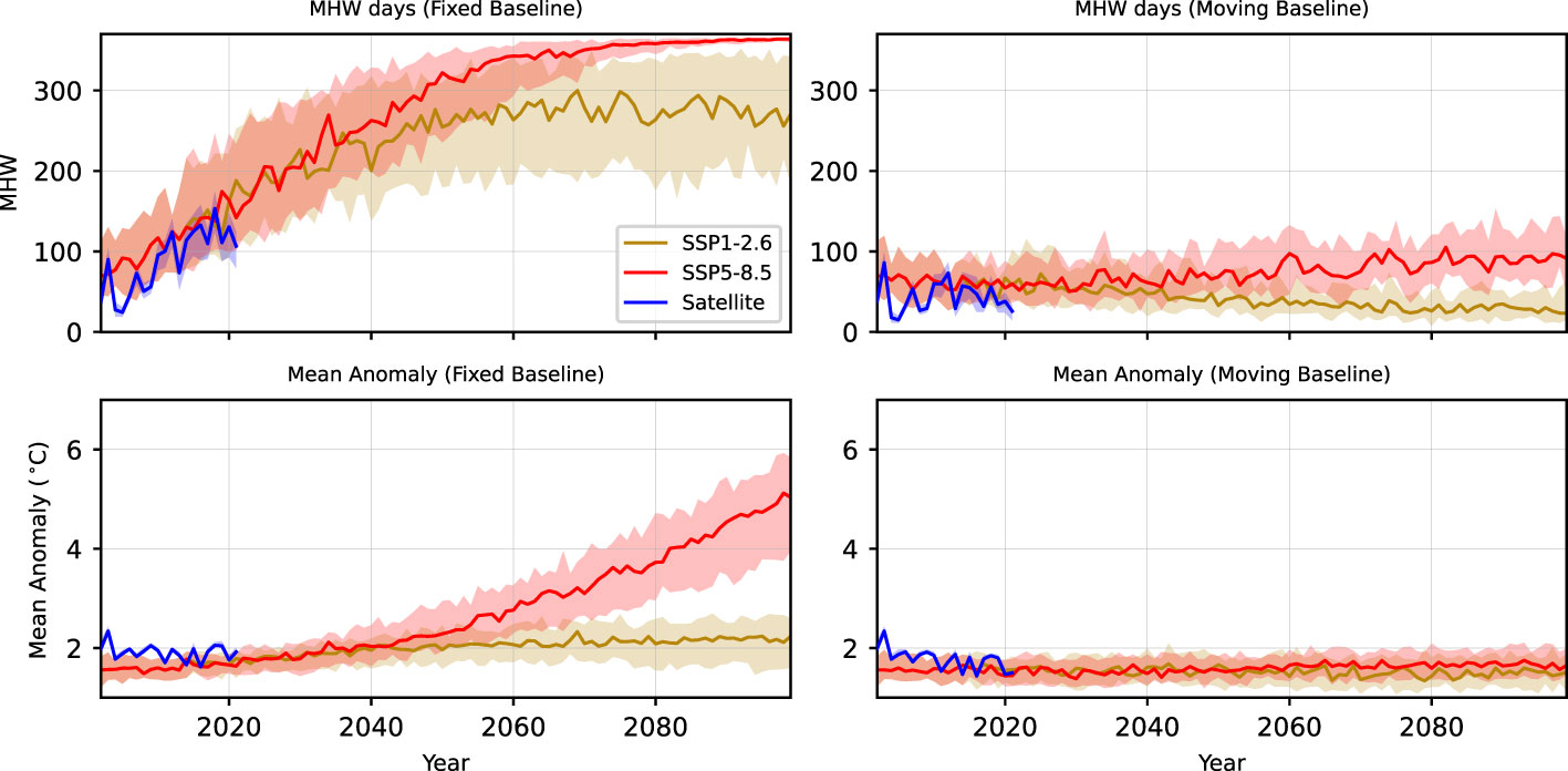
Figure 2 Number of MHW days per year and yearly mean MHW temperature anomaly in the Mediterranean Sea for fixed and moving baseline periods, comparing satellite SST data (blue) and CMIP6 models (red, yellow). (top-left) MHW days per year with a fixed baseline (1982–2001). (top-right) MHW days per year with a 20-year moving baseline. (bottom-left) Annual mean MHW anomaly using a fixed baseline. (bottom-right) Annual mean MHW anomaly using a moving baseline. Solid green and red lines represent the ensemble median for 22 CMIP6 models under the SSP1–2.6 and SSP5–8.5 scenarios, respectively. Red and yellow filled regions indicate the models’ ensemble 70% confidence intervals. The filled blue region corresponds to the interpolation error associated with the SST dataset.

Regarding the MHW anomaly (Figure 2), under the SSP5-8.5 scenario using a fixed baseline, the MHW anomaly exhibits an increasing trend, ultimately reaching a model ensemble mean value of 5.03 °C by the end of the century, with the 70% confidence interval being (3.95–5.83 °C). In contrast, for the SSP1-2.6 fixed baseline scenario, the anomaly plateaus at approximately 2.23 °C (1.60–2.60 °C) at the second half of the century. When employing a moving baseline, both the SSP5-8.5 and SSP1-2.6 scenarios maintain roughly constant values through the century of 1.59 °C (1.33–1.89°C) and 1.53 °C (1.23–1.85 °C), respectively.

MHW statistical values for a moving and a fixed baseline over the Mediterranean are shown in Figures 3, 4 respectively, including annual MHW day-count, anomaly and cumulative anomaly, and mean duration. Yearly mean values for this metric can be found at Table S1 in Supplementary Material. With a moving baseline, the average annual MHW day count for the Mediterranean for 2002 to 2021 is 43.1 days per year (31.6–54.0 days per year error range), which corresponds to 11.8% of the year, and does not show any significant temporal trend. Using a fixed baseline, the average annual MHW day count for the Mediterranean from 2002 to 2021 is 89.0 days per year (69.3–103.7 days per year error range), which corresponds to 24.4% of the year. The MHW day count has an increasing trend of 5.22 MHW days per year.

FIGURE 3

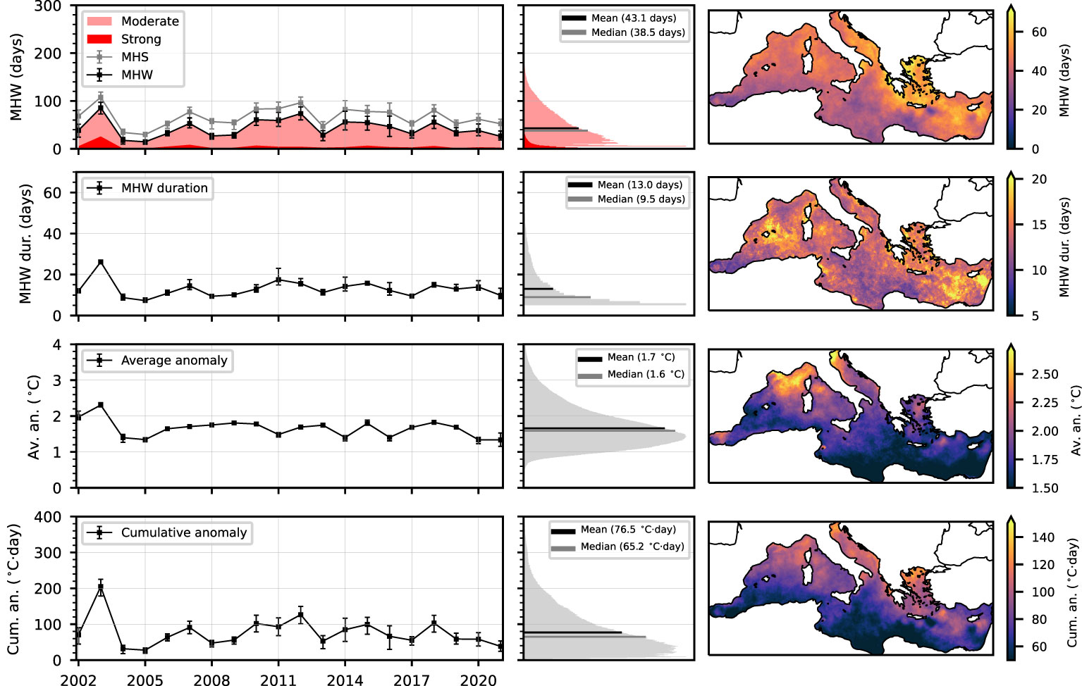
Figure 3 MHW statistical values for a moving baseline across the Mediterranean from satellite SST dataset. The rows represent the following metrics: MHW day-count (first row), event duration anomaly (second row), average MHW SST anomaly (third row), and cumulative MHW SST anomaly (fourth row). The columns display these metrics in different formats: annual time series of zonal averages (first column), total frequency distributions considering all MHW events and grid-points from 2002 to 2021 (second column), and spatial distributions over the Mediterranean basin, averaged for the 2002–2021 period (third column). Error bars indicate the uncertainty in the metrics due to the interpolation error in the SST dataset.

FIGURE 4

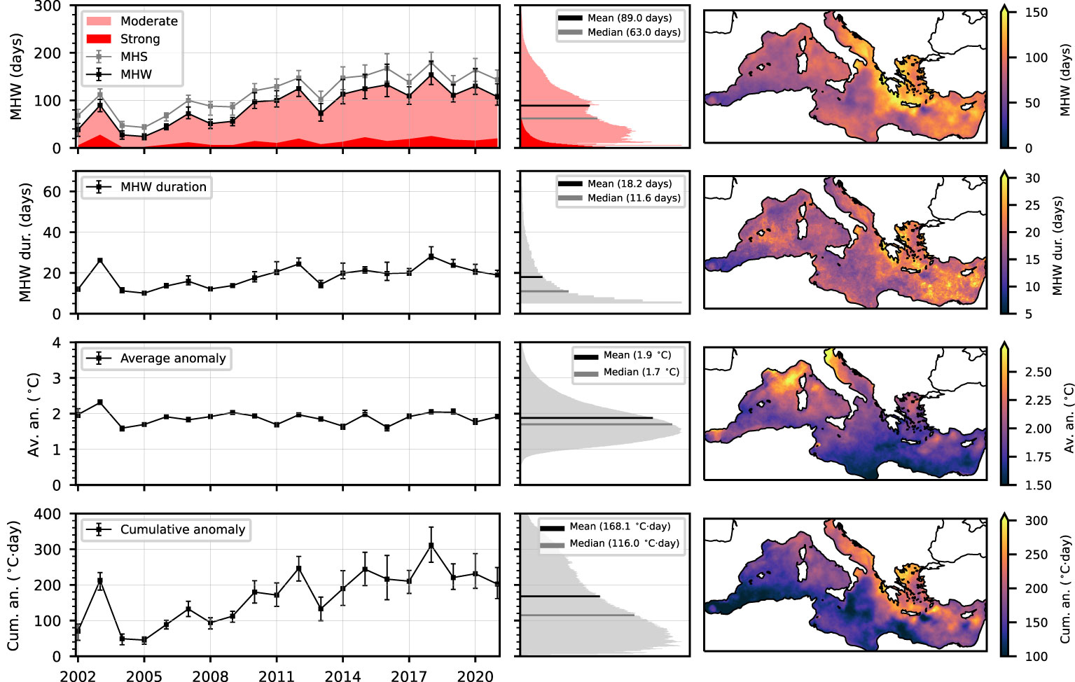
Figure 4 Same as Figure 3 but using the 1982–2001 fixed baseline.

Following the MHW intensity categorization proposed by Hobday et al. (2018), with each category defined as multiples of the value represented by the local difference between the climatological mean and the threshold, using a moving baseline most MHW events are moderate (I category). On average, 11.2% of MHW days have been strong events (II category) and 0.4% have been severe events (III category). With a fixed baseline strong and severe events average a 15.0% and 0.8% of all MHW days.

We used the Marine Heat Spike (MHS) day-count, defined as days when SST is above the MHW threshold but not necessarily contained in 5-day long waves, to compare the observed frequency of extreme events without the length constrain, with its expected theoretical value using a 90th percentile threshold (which is 10% of the year, or 35–36 days per year). For a moving baseline the mean annual MHS day-count value is 66.3 days per year (55.9-85.6 days per year error range), corresponding to 18.2% of the year, which is twice as high as one might initially expect. This disparity is attributable to the warming of the Mediterranean Sea, as the years analyzed have experienced warming with respect to the mean SST value of the baseline period, causing the MHS day-count to be higher than the expected theoretical value.

For a moving baseline, the mean MHW anomaly (degrees above climatological mean) is 1.66°C (1.66–1.70°C error range) with mean values above 2.50°C mostly on the north-western Mediterranean Sea and north Adriatic, both regions characterized by high calendar-day SST variability (not shown). Average mean annual cumulative intensity is 76.54°C·year (59.16–96.63 °C·year error range), with high values above 120°C·year mostly in the north Mediterranean, and lower values below 40°C·year mostly in the south Mediterranean. With a fixed baseline the mean MHW anomaly is slightly higher at 1.90°C (1.90–1.94°C error range) and the cumulative anomaly shows a trend of 9.25°C·year consistent with the trend in MHW days per year.

The duration of single MHW events is roughly uniformly distributed across the Mediterranean for a fixed and moving baseline. The most common duration for both baselines (statistical mode) is 5 days, with a mean value of 13.0 days for moving baseline (10.9–14.1 days error range) and 18.2 days for a fixed baseline (15.8–19.33 days error range). For a moving baseline, the distribution of MHW event duration decreases exponentially with the number of days, with 8.61% of events lasting more than a month (31 days); and on average, MHWs last longer in localized regions north of the Balearic Islands and east of Cyprus, both with mean values above 25 days per event.

The s ummer 2003 MHW, associated with an unprecedented atmospheric heat wave that struck Europe (García-Herrera et al., 2010), stands as the greatest MHW event in the Mediterranean as measured by all metrics considered only when considering a moving baseline (see Supplementary Table S1). If we use a fixed baseline, the accumulative secular warming of more recent years stands out as extreme with regard to MHW detection, as seen in Figure 4, where all 2012, 2014, 2015, 2016 and 2018 stand as years with a higher MHW annual day-count than 2003.

5 Discussion

In the context of anthropogenic climate change and rising awareness about the perils of extreme climate events, an indicator for detecting MHWs offers a valuable resource to assess the impacts of extreme sea temperature events. The study of MHWs has a wide range of applications, from a gauge for ecological and socioeconomic impacts to a climate change indicator, which satisfy differing scientific interests and end-user needs. As a consequence of this broad applicability, different definitions of extreme temperature events, all encompassed within the term “marine heat wave”, may be used to serve different purposes. Within statistical definitions of MHWs (as opposed to using case-specific absolute thresholds) variability in the definition may arise from the criteria used to define the threshold (e.g., 90th percentile or 99th percentile of the baseline distribution), the temporal scale (e.g., daily or monthly), the minimum duration required for an event to be considered as such (5 days or more, with or without filling 2-day gaps), and the choice of the baseline climatological period, which can be either fixed in the past or shifted in time.

With regard to the rarity of MHWs, one could argue that the current definition of MHW with a 90th percentile threshold results in events that are too frequent for them to be classified as extreme SST events, even with a moving baseline, as the average MHW days per year in the Mediterranean corresponds to 13% of the year. In comparison, the Intergovernmental Panel on Climate Change (IPCC) defines warm days and cold nights with 10th and 90th percentile thresholds, respectively, for atmospheric temperature, and they may not be necessarily considered extreme in nature (Murray and Ebi, 2012). Whether this is the case or not, the intensity categorization provided by Hobday et al. (2018) built on top of the standard definition of MHWs offers a reliable gauge to account for rarer, more extreme events.

In conclusion, MHWs serve as a valuable indicator to assess the impact of extreme events, and the choice between a fixed or moving baseline should be guided by the intended focus on ecosystem adaptation (Holbrook et al., 2020). Both fixed and moving baselines can be employed separately or in conjunction to highlight the long timescale impacts (fixed baseline) and short timescale impacts (moving baseline) of extreme SST events. In this context, we value the approach presented by Amaya et al. (2023) who emphasize the need to differentiate between long-term temperature trends and marine heatwaves, advocating for the use of an evolving baseline definition. Although some may argue that a fixed baseline challenges the characterization of these events as ‘extreme,’ it is important to consider the specific context and goals of the study. If the priority is to establish a consistent MHW definition that allows for uniform results across space (facilitating regional comparisons) and time (enabling equitable comparison of events years apart), we recommend considering the following factors: 1. A statistical definition of MHW, which promotes fair comparisons across various regions. 2. A moving baseline, as it results in events with a consistent basal frequency overtime and prevents the saturation of annual MHW day-count in the context of a warming sea. However, researchers should carefully weigh the advantages and limitations of both fixed and moving baselines in relation to their specific objectives.

This study represents an initial effort to provide MHW statistics in the Mediterranean Sea for both fixed and moving baselines. However, there remains ample opportunity for future research to expand upon these findings. Further investigation could consider alternative baseline periods and definitions of extreme events, as well as the incorporation of more sophisticated detrending techniques to account for long-term climate trends. By doing so, subsequent studies may provide additional insight into the complex interplay between MHWs, ecosystem adaptation, and the choice of baseline methodologies. This research serves as a foundation upon which more nuanced understandings of marine heatwave dynamics in the Mediterranean Sea can be built, ultimately guiding regional conservation and management efforts more effectively.

Data availability statement

The datasets presented in this study can be found in online repositories. The names of the repository/repositories and accession number(s) can be found below: Repository: MHW_moving_fixed (https://github.com/canagrisa/MHW_moving_fixed) DOI: 10.5281/zenodo.7908932.

Author contributions

PR contributed to the data processing, analysis of results, and writing of the manuscript. AP contributed to the conception of this study, its supervision, and obtained the funding to develop this research. VC contributed to the data processing of model data, and scientific discussion. All authors contributed to the article and approved the submitted version.

Funding

This work has been funded by the JAE-Intro scholarships issued by the Spanish National Research Council (CSIC), the Mediterranean Institute for Advanced Studies (IMEDEA), and the University of Balearic islands (UIB). Part of this work was supported by the EuroSea project (www.eurosea.eu), which has received funding from the European Union’s Horizon 2020 Research and Innovation Programme under grant agreement No. 862626.

Acknowledgments

The present research was carried out within the framework of the activities of the Spanish Government through the "María de Maeztu Centre of Excellence" accreditation to IMEDEA (CSIC-UIB) (CEX2021- 001198). We would like to thank insightful discussions with the following colleagues: M. Juza, S. Speich, H. Dayan, R. James, N. Marbà and I. Hendricks. VC also acknowledges the support from the Ramón y Cajal Program (RYC2020-029306-I) and from the European Social Fund/Universitat de les Illes Balears/Spanish State Research Agency (AEI - 10.13039/501100011033). The authors also thank the four reviewers for their insightful comments and suggestions.

Conflict of interest

The authors declare that the research was conducted in the absence of any commercial or financial relationships that could be construed as a potential conflict of interest.

Publisher’s note

All claims expressed in this article are solely those of the authors and do not necessarily represent those of their affiliated organizations, or those of the publisher, the editors and the reviewers. Any product that may be evaluated in this article, or claim that may be made by its manufacturer, is not guaranteed or endorsed by the publisher.

Supplementary material

The Supplementary Material for this article can be found online at: https://www.frontiersin.org/articles/10.3389/fmars.2023.1168368/full#supplementary-material

Footnotes

1. ^ https://resources.marine.copernicus.eu/product-detail/SST_MED_SST_L4_REP_OBSERVATIONS_010_021/INFORMATION
2. ^ For a recent critique about this criteria, see [(Jacox et al., 2020) ]

References

Amaya D., Jacox M. G., Fewings M. R., Saba V. S., Stuecker M. F., Rykaczewski R. R., et al. (2023). Marine heatwaves need clear definitions so coastal communities can adapt. Nature 616, 29–32. doi: 10.1038/d41586-023-00924-2

CrossRef Full Text | Google Scholar

Dayan H., McAdam R., Juza M., Masina S., Speich S. (2023). Marine heat waves in the mediterranean sea: an assessment from the surface to the subsurface to meet national needs. Front. Mar. Sci. 10, 142. doi: 10.3389/fmars.2023.1045138

CrossRef Full Text | Google Scholar

Donlon C. J., Martin M., Stark J., Roberts-Jones J., Fiedler E., Wimmer W. (2012). The operational sea surface temperature and sea ice analysis (ostia) system. Remote Sens. Environ. 116, 140–158. doi: 10.1016/j.rse.2010.10.017

CrossRef Full Text | Google Scholar

Eyring V., Bony S., Meehl G. A., Senior C. A., Stevens B., Stouffer R. J., et al. (2016). Overview of the coupled model intercomparison project phase 6 (cmip6) experimental design and organization. Geosci. Model. Dev. 9, 1937–1958. doi: 10.5194/gmd-9-1937-2016

CrossRef Full Text | Google Scholar

Frölicher T. L., Fischer E. M., Gruber N. (2018). Marine heatwaves under global warming. Nature 560, 360–364. doi: 10.1038/s41586-018-0383-9

CrossRef Full Text | Google Scholar

García-Herrera R., Díaz J., Trigo R. M., Luterbacher J., Fischer E. M. (2010). A review of the european summer heat wave of 2003. Crit. Rev. Environ. Sci. Technol. 40, 267–306. doi: 10.1080/10643380802238137

CrossRef Full Text | Google Scholar

Hansen J., Ruedy R., Sato M., Lo K. (2010). Global surface temperature change. Rev. Geophys. 48 (4), 1–3. doi: 10.1029/2010RG000345

CrossRef Full Text | Google Scholar

Hobday A. J., Alexander L. V., Perkins S. E., Smale D. A., Straub S. C., Oliver E. C., et al. (2016). A hierarchical approach to defining marine heatwaves. Prog. Oceanogr. 141, 227–238. doi: 10.1016/j.pocean.2015.12.014

CrossRef Full Text | Google Scholar

Hobday A. J., Oliver E. C. J., Gupta A. S., Benthuysen J. A., Burrows M. T., Donat M. G., et al. (2018). Categorizing and naming marine heatwaves. Oceanography 31, 162–173. doi: 10.5670/oceanog.2018.205

CrossRef Full Text | Google Scholar

Holbrook N. J., Sen Gupta A., Oliver E. C., Hobday A. J., Benthuysen J. A., Scannell H. A., et al. (2020). Keeping pace with marine heatwaves. Nat. Rev. Earth Environ. 1 (9), 482–493. doi: 10.1038/s43017-020-0068-4

CrossRef Full Text | Google Scholar

Jacox M. G. (2019). Marine heatwaves in a changing climate. Nature 571, 486. doi: 10.1038/d41586-019-02196-1

CrossRef Full Text | Google Scholar

Jacox M. G., Alexander M. A., Bograd S. J., Scott J. D. (2020). Thermal displacement by marine heatwaves. Nature 584, 82–86. doi: 10.1038/s41586-020-2534-z

CrossRef Full Text | Google Scholar

Juza M., Fernández-Mora À., Tintoré J. (2022). Sub-Regional marine heat waves in the mediterranean sea from observations: long-term surface changes, sub-surface and coastal responses. Front. Mar. Sci. 9. doi: 10.3389/fmars.2022.785771

CrossRef Full Text | Google Scholar

Juza M., Tintoré J. (2021). Multivariate sub-regional ocean indicators in the mediterranean sea: from event detection to climate change estimations. Front. Mar. Sci. 8, 610589. doi: 10.3389/fmars.2021.610589

CrossRef Full Text | Google Scholar

Klein Tank A. M. G., Zhang X., Zwiers F. W., World Meteorological Organization (2009). Guidelines on analysis of extremes in a changing climate in support of informed decisions for adaptation. (WMO), 14–15.

Google Scholar

Kriegler E., Edmonds J., Hallegatte S., Ebi K. L., Kram T., Riahi K., et al. (2014). A new scenario framework for climate change research: the concept of shared climate policy assumptions. Climatic Change 122, 401–414. doi: 10.1007/s10584-013-0971-5

CrossRef Full Text | Google Scholar

Marbà N., Duarte C. M. (2010). Mediterranean Warming triggers seagrass (posidonia oceanica) shoot mortality. Global Change Biol. 16, 2366–2375. doi: 10.1111/j.1365-2486.2009.02130.x

CrossRef Full Text | Google Scholar

Merchant C. J., Embury O., Bulgin C. E., Block T., Corlett G. K., Fiedler E., et al. (2019). Satellite-based time-series of sea-surface temperature since 1981 for climate applications. Sci. Data 6, 1–18. doi: 10.1038/s41597-019-0236-x

CrossRef Full Text | Google Scholar

Murray V., Ebi K. L. (2012). Ipcc special report on managing the risks of extreme events and disasters to advance climate change adaptation (srex). J. Epidemiol. Community Health 66, 759–760. doi: 10.1136/jech-2012-201045

CrossRef Full Text | Google Scholar

Oliver E. C. (2019). Mean warming not variability drives marine heatwave trends. Climate Dyn. 53, 1653–1659. doi: 10.1007/s00382-019-04707-2

CrossRef Full Text | Google Scholar

Oliver E. C., Donat M. G., Burrows M. T., Moore P. J., Smale D. A., Alexander L. V., et al. (2018). Longer and more frequent marine heatwaves over the past century. Nat. Commun. 9, 1–12. doi: 10.1038/s41467-018-03732-9

CrossRef Full Text | Google Scholar

Pisano A., Ciani D., Marullo S., Santoleri R., Buongiorno Nardelli B. (2022). A new operational mediterranean diurnal optimally interpolated sst product within the copernicus marine environment monitoring service. Earth Sys. Sci. Data Dis. 1–26. doi: 10.5194/essd-2021-462

CrossRef Full Text | Google Scholar

Pisano A., Nardelli B. B., Tronconi C., Santoleri R. (2016). The new mediterranean optimally interpolated pathfinder avhrr sst dataset, (1982–2012). Remote Sens. Environ. 176, 107–116. doi: 10.1016/j.rse.2016.01.019

CrossRef Full Text | Google Scholar

Rey J., Rohat G., Perroud M., Goyette S., Kasparian J. (2020). Shifting velocity of temperature extremes under climate change. Environ. Res. Lett. 15, 034027. doi: 10.1088/1748-9326/ab6c6f

CrossRef Full Text | Google Scholar

Riahi K., van Vuuren D. P., Kriegler E., Edmonds J., O’Neill B. C., Fujimori S., et al. (2017). The shared socioeconomic pathways and their energy, land use, and greenhouse gas emissions implications: an overview. Global Environ. Change 42, 153–168. doi: 10.1016/j.gloenvcha.2016.05.009

CrossRef Full Text | Google Scholar

Secretariat (2019). Technical regulations. volume 1: general meteorological standards and recommended practices (World Meteorological Organization), xiv.

Google Scholar

Soga M., Gaston K. J. (2018). Shifting baseline syndrome: causes, consequences, and implications. Front. Ecol. Environ. 16, 222–230. doi: 10.1002/fee.1794

CrossRef Full Text | Google Scholar

Stephenson D. B., Diaz H., Murnane R. (2008). Definition, diagnosis, and origin of extreme weather and climate events. Climate Extremes Soc. 340, 11–23. doi: 10.1017/CBO9780511535840.004

CrossRef Full Text | Google Scholar

Stocker T. F., Qin D., Plattner G.-K., Alexander L. V., Allen S. K., Bindoff N. L., et al. (2013). “Technical summary,” in Climate change 2013: the physical science basis. contribution of working group I to the fifth assessment report of the intergovernmental panel on climate change (Cambridge University Press), 109–110.

Google Scholar

Trewin B. C. (2007). The role of climatological normals in a changing climate (World Meteorological Organization WMO/TD) 6.

Google Scholar

WMO (2012). Guide to climatological practices (World Meteorological Organization), 759–760.

Google Scholar