Spatial dynamics of Maine lobster landings in a changing coastal system

1 Introduction

Warming oceans have caused global shifts in the distributions of many marine species as thermal habitats become unfavorable and even exceed physiological thresholds (Cheung et al., 2016; Schuetz et al., 2019). Continued warming is expected to significantly impact global fisheries catch, both spatially and temporally (Cheung et al., 2016). Changes in fisheries catch due to warming oceans can have widespread impacts on fisheries and fishing-dependent communities, altering resource use and income opportunities (Cheung et al., 2016; Greenan et al., 2019). The threat of a warming ocean to fisheries calls for an improved understanding of the effects of climate change on fisheries output for future management and adaptation to environmental change.

Environmental parameters, such as climate, often can affect fisheries output and performance by influencing a fish stock’s abundance, health, and distribution (Cushing, 1982; Lehodey et al., 2006; NOAA, Fisheries, 2013). Changes in environmental parameters can alter the quality and distribution of suitable habitats for a given stock. The state of a fish stock may affect the fleet dynamics, distribution, and efficiency of fishing effort, which subsequently alters fishery performance and output (Franklin, 2010). Therefore, it is essential to understand how changes in environmental conditions affect species distribution. Proxies, such as changes in habitat quality and distribution of suitable habitat, are often used to estimate the state and distribution of a given stock (Brown et al., 2000; Tanaka and Chen, 2016; Rowden et al., 2017).

Researchers frequently use a bioclimate envelope (BE) model, a predictive spatial model, to forecast the suitability and distribution of habitat for a species based on influential environmental variables (Xue et al., 2017; Tanaka et al., 2019). Estimates of habitat suitability can be used to infer a given stock’s spatial distribution and abundance (Morris and Ball, 2006; Tanaka et al., 2019). For this study, we use the American lobster (Homarus americanus) fishery in the state of Maine, U.S., as a case study for exploring historical and forecasted connections between environmental variables and fisheries output defined as fishery landings by pounds.

The American lobster fishery is one of the most valuable fisheries in the U.S., with more than 80% of U.S. landings occurring in Maine state waters (Maine Department of Marine Resources (MEDMR), 2020). Around 98% of Gulf of Maine landings come from “near shore” areas defined as 0-12 miles from the coast (Atlantic States Marine Fisheries Commission (ASMFC) American Lobster Stock Assessment Review Panel, 2020). In addition, this fishery is a significant economic driver and source of cultural identity in coastal Maine (Acheson, 1988; Donihue, 2018). The Maine lobster fishery is unique in that despite the small-scale, input-limited nature of operation, the fishery operates at an incredible scale of around 4,500 active individual licenses throughout the state (Maine Department of Marine Resources (MEDMR), 2020; Atlantic States Marine Fisheries Commission (ASMFC) American Lobster Stock Assessment Review Panel, 2020). This results in a diverse, individualized structure of the fishery which is reflected in the spatial distribution of different fishing behaviors, strategies, and landings (Acheson, 1988; Maine Department of Marine Resources (MEDMR), 2020; Atlantic States Marine Fisheries Commission (ASMFC) American Lobster Stock Assessment Review Panel, 2020).

The fishery has experienced a dramatic increase in landings since the late 1980’s, known as the “lobster boom” which correlates changes in lobster abundance regimes (Atlantic States Marine Fisheries Commission (ASMFC) American Lobster Stock Assessment Review Panel, 2020). This increase is often attributed to rising temperatures, immigration from southern New England, decreased predation from other species, bait input, and highly effective management and conservation strategies that protect reproductive female lobsters (Grabowski et al., 2010; Le Bris et al., 2018; Mazur et al., 2020).

These increases in landings are reflected in increases in American lobster abundance in the Gulf of Maine (GoM) and Georges Bank (GBK) over the past 50 years. The American lobster stock is observed to have undergone two abundance regime shifts from a low abundance regime (before 1995) to moderate abundance regime (1996-2008) to currently a high abundance regime (2009-present) (Atlantic States Marine Fisheries Commission (ASMFC) American Lobster Stock Assessment Review Panel, 2020). As exothermic mobile crustaceans, American lobsters are sensitive to environmental parameters, notably temperature and salinity, and seek favorable conditions and habitats (Tanaka and Chen, 2016; Atlantic States Marine Fisheries Commission (ASMFC) American Lobster Stock Assessment Review Panel, 2020). Previous studies suggest a northeast and further from shore migration of American lobsters, which is reflected in seasonal fishing behaviors (Boenish and Chen, 2017; Rheuban et al., 2017 Kleisner et al., 2017). In addition, the GoM has been experiencing its most intense warming period in the past 50 years due to the indirect effects of greenhouse gasses and resulting oceanographic processes (Pershing et al., 2015; Jewett and Romanou, 2017). Changes in environmental parameters are expected to impact the quality and distribution of suitable habitat for American lobster and fishery landings (Rheuban et al., 2017; Tanaka et al., 2019; Behan et al., 2021). Understanding the relationship between current and past environments and current and past habitat suitability can provide insights into future distributions of suitable habitats for American lobster. Therefore, evaluating spatio-temporal dimensions of how environmental parameters affect suitable habitats for lobsters will improve understanding of the overall spatio-temporal distribution of lobsters and fishery landings in the GoM.

This study aims to connect spatio-temporal distributions of climate-driven suitable lobster habitat with the distribution of landings across lobster management zones. We modified a bioclimate envelope model for American lobster, initially developed by Tanaka and Chen (2016), to project spatio-temporal distributions of American lobster habitat using long-term, fine-scale environmental data. We built a generalized additive model (GAM) to interpolate fishery landings from projected lobster habitats. We then used forecasted environmental conditions based on different climate change scenarios to estimate future distributions of landings for the Maine lobster fishery. We extend the literature on climate-driven American lobster habitat and fishery output in two important dimensions. First, we expand upon early work on the habitat suitability of American lobsters (Tanaka and Chen, 2016; Behan et al., 2021) to incorporate a management-specific scale distinct within the inshore GoM (Rheuban et al., 2017). We also explicitly connect environmental parameters to fishery output (Xue et al., 2007; Oppenheim et al., 2019) and compare across historical and forecasted time scales (Boenish and Chen, 2017). This work highlights the importance of considering climate influences in evaluating fishery performance.

2 Methods

2.1 Maine-New Hampshire inshore trawl survey

The Maine-New Hampshire Inshore Trawl Survey (Figure 1) was used as a fishery-independent source of habitat and abundance data to inform the BE model. The survey is a seasonal, semi-annual trawl that provides catch (abundance) data with the habitat variables of temperature, salinity, depth, and location (latitude/longitude) (Sherman et al., 2005). The survey is jointly coordinated by the Maine Department of Marine Resources (Maine Department of Marine Resources (MEDMR), 2020) and the New Hampshire Fish and Game Department (NHFGD) and is split seasonally into a Spring (April-June) and Fall (September-November) survey. The survey follows a stratified random sampling design along the coast of Maine and New Hampshire, consisting of four depth strata (5-20, 21-35, 36-55, and 56+ fathoms) (9.14–36.6, 38.4- 64.0, 65.8-101, and 102+ meters).The survey stays within the “near shore” boundary of 0-12 nautical miles (NM) from shore and encompasses both state waters (“inshore”) boundary of 0-3 NM from shore and part of federal water (“offshore”) boundary of 3-200 NM from shore (Sherman et al., 2005; Atlantic States Marine Fisheries Commission (ASMFC) American Lobster Stock Assessment Review Panel, 2020). A modified shrimp trawl with 50.8 millimeters (mm) mesh wings and 12.7 mm mesh cod end is towed for 20 minutes at 2.2-2.3 knots (4.07-4.25 kilometers per hour) to cover approximately 1.5 kilometers² (km²) per tow. The survey targets 115 stations per season, approximating a sampling density of 1 station every 40 NM² (137.2 km²) (Sherman et al., 2005).

FIGURE 1

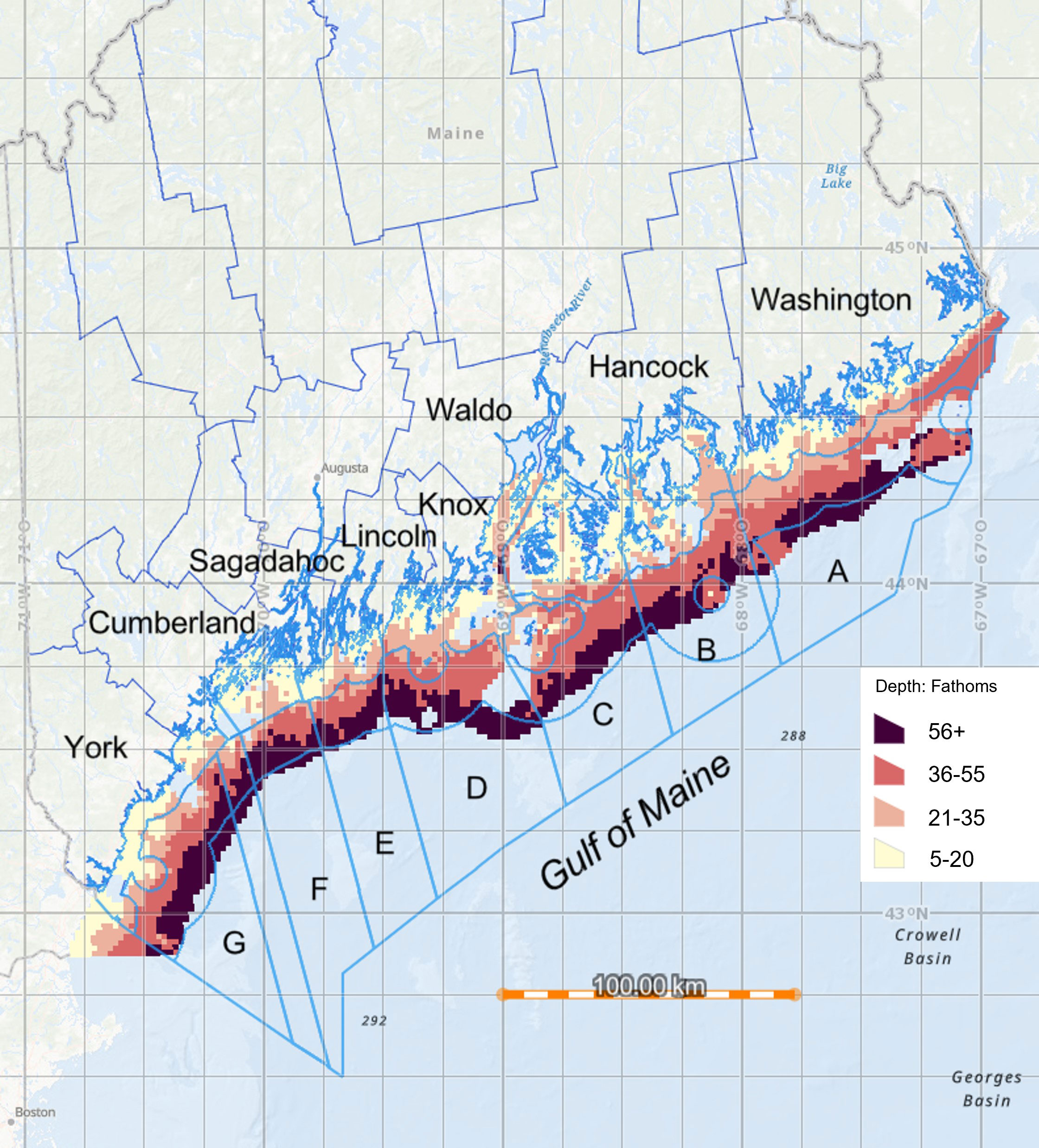
Figure 1 Regional and depth strata of survey region for the Maine – New Hampshire Inshore Trawl Survey. Adapted from “Maine- New Hampshire Inshore Groundfish Trawl Survey Procedures and Protocols,” Shows county and zones (A-G) of survey area. Figure created using ArcGIS.

2.2 Environmental data

The Finite Volume Community Ocean Model (FVCOM) is an open source, fine-scale ocean circulation model developed by the Marine Ecosystem Dynamics Modelling (MEDM) lab at the University of Massachusetts Dartmouth and the Woods Hole Oceanographic Institution, and is often used to model habitat and oceanographic data in the Northwest Atlantic (Chen et al., 2005). We pulled bottom temperature, bottom salinity, and depth using midday (12:00 pm) of every 4^th day for Spring (April-June) and Fall (September – November) 1978-2018. We pulled different seasonal data to best match the seasonality of the MENH Inshore Trawl Survey. The total area pulled covered 128,400 km² a grid scale of 0.01 decimal degrees² (1.11 km²) (Li et al., 2017; Behan et al., 2021). The finite volume unstructured grid of FVCOM has been shown to accurately represent the environmental variables of Maine’s long coastline with observed data at this fine scale (Li et al., 2017). Environmental data from FVCOM was spatially interpolated onto the fine-scale unstructured FVCOM grid using bivariate spline interpolation through the “akima” package and the “raster” package in R (Hijmans and van Etten, 2012; Akima and Gebhardt, 2016). Further detail on the interpolation process is described in section 2.4 in Methods.

2.3 IPCC carbon emission scenario data

Data from the Intergovernmental Panel on Climate Change (IPCC) were used to estimate future bottom temperature and bottom salinity data for the Representative Concentration Pathway (RCP) 4.5 and 8.5 carbon emission scenarios. The different RCP scenarios 4.5 (climate policy) and 8.5 (business-as-usual) serve as forecasting benchmarks for future temperature and salinity habitat variables. Forecasted habitat variables are calculated from changes in averages, called anomalies, from the NOAA historical baselines period (1956-2005) and are estimated for the future time periods 2006-2055 and 2050-2099. However, our FVCOM historical baseline period (1978-2005) does not match the NOAA historical baseline. We delta-downscaled IPCC anomalies by interpolating anomalies to the same FVCOM grid using the same bivariate spline interpolation methods used for the FVCOM environmental data. Anomalies were then applied to our FVCOM baseline to forecast bottom temperature and salinity to the periods 2028-2055 and 2072-2099. We assume depth, latitude, and longitude do not change over time. Similar delta-downscaling and interpolation methods can be found in the methods by Behan et al. (2021). Interpolation methods are further described in the following section 2.4.

2.4 Bioclimate envelope model

The bioclimate envelope (BE) model for American lobster, first developed by Tanaka and Chen (2016), estimates suitable habitat distributions in the GoM from habitat variables and has been used previously to estimate habitat suitability and infer species abundance and distribution. Bottom temperature and bottom salinity have been previously identified as key habitat variables (Tanaka and Chen, 2016). Depth, latitude, and longitude are used as habitat spatial variables to capture spatial differences of habitat in the diagonal direction of the Maine coast as well as the differences between inshore and offshore habitats. Substrate data was considered, but ultimately not used as the trawl survey is inherently biased toward softer bottoms, and the scale of the substrate data was not fine enough for our analysis (Sherman et al., 2005; Behan et al., 2021). The BE model predicts habitat suitability for American lobster from survey catches (abundance) and habitat variables using fisheries-independent survey data and can be used to infer species abundance and distribution given habitat. The BE model builds a suitability index for each habitat variable based on survey catch, latitude, and longitude, and modelled FVCOM bottom temperature and botton salinity for the same latitude and longitude of the survey. Modelled FVCOM environmental variables were spatially interpolated using “akima” package in R, which allows for bivariate cubic splines of gridded data (Akima and Gebhardt, 2016). We filled the rest of the FVCOM grid using raster interpolation through “raster” package in R, which creates a continuous surface from sampled point values (Hijmans and van Etten, 2012). IPCC anomalies were delta downscaled using the same spatial interpolation method and applied to our FVCOM baseline. Interpolated habitat variables were then used as input into the BE model to create a suitability index for the interpolated values of each habitat variable. The suitability indices are then averaged to obtain an overall habitat suitability index map. The BE modelhas since been modified and used in multiple studies regarding lobster habitat suitability in the GoM and surrounding regions to improve management decisions (Behan et al., 2021; Hodgdon et al., 2021; Tanaka et al., 2020). This version of the BE model was adapted from the Behan et al. (2021) model and modified to fit our data structure and study region and follows similar methodology for data extraction, model building, and interpolation.

Separate BE models were built using spring (April-June) and fall (September-November) survey data to capture seasonal variability, which has previously been shown to be important for bioclimate envelope models for American lobsters (Hodgdon et al., 2021). This is important as lobsters migrate seasonally inshore during the summer and fall to reproduce, and offshore during the winter and spring (Atlantic States Marine Fisheries Commission (ASMFC) American Lobster Stock Assessment Review Panel, 2020). FVCOM and IPCC interpolated data were used by the BE models to estimate habitat suitability in the inshore GoM for spring and fall.

2.4.1 Suitability index

Suitability indices (SIs) for each of the identified habitat variables were first developed using the ME-NH inshore trawl survey data. A combination of variance inflation factors (VIF) testing and correlation matrices were used to maximize our dependent variables. Each variable was split into 14 Fisher’s natural breaks classes (k) following the methods of Behan et al. (2021). Suitability indices (SI) for each k for each habitat variable were calculated as such:

$$S{I}_{\left\{k,i\right\}} =(Catc{h}_{\left\{k,i\right\}}- Catc{h}_{\left\{i,min\right\}})/(Catc{h}_{\left\{i,max\right\}}- Catc{h}_{\left\{i,min\right\}})$$

where Catch_min and Catch_max are minimum and maximum catch from the survey for each k of each variable. As there is only one survey used, unit effort is consistent and thus abundance from the survey can be used as catch per unit effort (CPUE). This establishes SI’s ranging from 0 (unsuitable) to 1 (most suitable) for each habitat variable (Tanaka and Chen, 2016; Behan et al., 2021). Generalized additive models (GAMs) were used to smooth the relationship between each k for each variable such that SI’s become a smooth continuous range from 0-1 for each k of habitat variable. Habitat variables from FVCOM and the IPCC were interpolated into he BE model to create SI maps of each habitat variable at the same fine scale FVCOM grid.

2.4.2 Habitat suitability index

Resulting SI’s were then averaged using an arithmetic mean with equal weights to estimate an overall Habitat Suitability Index (HSI) of the same scale of 0 to 1 (Hodgdon et al., 2021; Tanaka et al., 2020). Spatially explicit HSI maps were created using the same fine-scale FVCOM grid (Xue et al., 2017; Behan et al., 2021). Bottom temperature and bottom salinity from FVCOM were used to interpolate HSI maps for the inshore Gulf of Maine for historical (1978–2005) and current (2004–2017) time periods. Forecasted bottom temperature and bottom salinity from the IPCC were used to interpolate HSI maps for forecasted (2028-2055; 2072-2099) time periods. HSI was then spatially divided into the Maine lobster management zones and averaged using a geometric mean to estimate HSI per zone, per time period, for fall and spring seasons.

2.5 The Maine lobster fishery

The Maine lobster fishery is an input-controlled, trap-exclusive, and limited entry and crew fishery. Each license holder is able to fish up to 800 traps, except for Zone E, which has a maximum limit of 600 traps. There is a maximum crew size of 3 people (including captain). Entry into the fishery consists of one new license for every ten exit of licenses, with new licenses including those obtained through apprentenceship (student license). The majority of fishers land their catch inshore during the summer and fall seasons when lobsters are plentiful and close to shore. However, the fishery can operate year round with some fishers choosing to fish offshore during winter and spring in deeper waters further from shore for a lower catch, but higher seasonal price (Atlantic States Marine Fisheries Commission (ASMFC) American Lobster Stock Assessment Review Panel, 2020). Only about 20% of the fishery owns a federal fishing license which allows one to fish offshore beyond 3NM from shore (Atlantic States Marine Fisheries Commission (ASMFC) American Lobster Stock Assessment Review Panel, 2020). Therefore we make the assumption that the Maine lobster fishery is primarily an inshore and summer/fall fishery despite being an year round fishery with access to offshore fishing grounds.

2.5.1 Fishery landings

We used publicly available annual landings by coastal county (1964-2019) and lobster management zone (2004-2019) from the Maine DMR. Landings data is collected by the Maine DMR annually using a 100% dealer reporting and a 10% harvester reporting framework at a scale of county, zone, month, and year (Maine Department of Marine Resources (MEDMR), 2020). Before the year 2004, the data is only available at the scale of county and year. As the vast majority of landings are caught in the summer and fall, we assume that the combined annual landings can encompass both spring and fall seasonal fishery biological processes (Maine Department of Marine Resources (MEDMR), 2020; Atlantic States Marine Fisheries Commission (ASMFC) American Lobster Stock Assessment Review Panel, 2020). Although vessel size, gear restrictions, fishing effort, and fishing capacity have shifted over time (ASMFC, 2020), the fundamental fishing method using traps has stayed consistent during our study period and is likely to persist into the future (Acheson, 1988; McClenachan et al., 2020). As such, we assume that fishery landings are comparable across time scales for both hindcasting and forecasting. Fishing effort follows seasonal and long-term migrations of lobster distributions (Chen et al., 2005; Boenish and Chen, 2017; Rheuban et al., 2017). Therefore, we assume that the fishery behaves as a pursuit fishery, where distribution of landings reflect the distribution of lobsters in the GoM. There is a minimum (82.5 milimeter carpace length) and maximum (127 milimeter carapace length) legal size, but the majority of lobsters landed are at the minimum legal size. Thus, we assume the Maine lobster fishery behaves as a recruitment fishery, where there is a consistent homogeneity of size of catch (Steneck and Wilson, 2001; Chen et al., 2005; Atlantic States Marine Fisheries Commission (ASMFC) American Lobster Stock Assessment Review Panel, 2020). The pursuit and recruitment nature of the fishery allows us to make the important assumption that fishery landings reflect a consistent level of local fishable biomass. We determined that a post “lobster boom” period better reflects the current fishery dynamics of warmer temperatures, established management practices, high recruitment, low predator abundance, and higher fishing capacity (Atlantic States Marine Fisheries Commission (ASMFC) American Lobster Stock Assessment Review Panel, 2020).

2.5.2 County and zone spatial delineation

There are 8 coastal counties which contribute to the state commercial fishery. Currently, the fishery is co-managed in 7 (A-G) lobster management zones in the inshore Gulf of Maine (Figure 2), which are based on de facto existing social boundaries within the fishery (Acheson et al., 2000). Zone boundaries encompass both inshore and offshore regions, but do not exceed the federal Exclusie Economic Zone Management Area 1 (Atlantic States Marine Fisheries Commission (ASMFC) American Lobster Stock Assessment Review Panel, 2020). Coastal Maine is often divided into three regions based on social and physical geography, including Southcoast (southwest part of the coast, Zones F and G, counties Cumberland and York); Midcoast (middle part of the coast up to Penobscot Bay, Zones D and E, counties parts of Knox and Waldo, Lincoln, and Sagadahoc); and Downeast (northeast part of coast past Penobscot Bay, Zones A, B, and C, counties, Washington, Hancock, parts of Knox and Waldo). Zone and county groupings into regions are based on that of the Maine Lobstermen’s Community Alliance (MLCA, https://bit.ly/3HS8nr0).

FIGURE 2

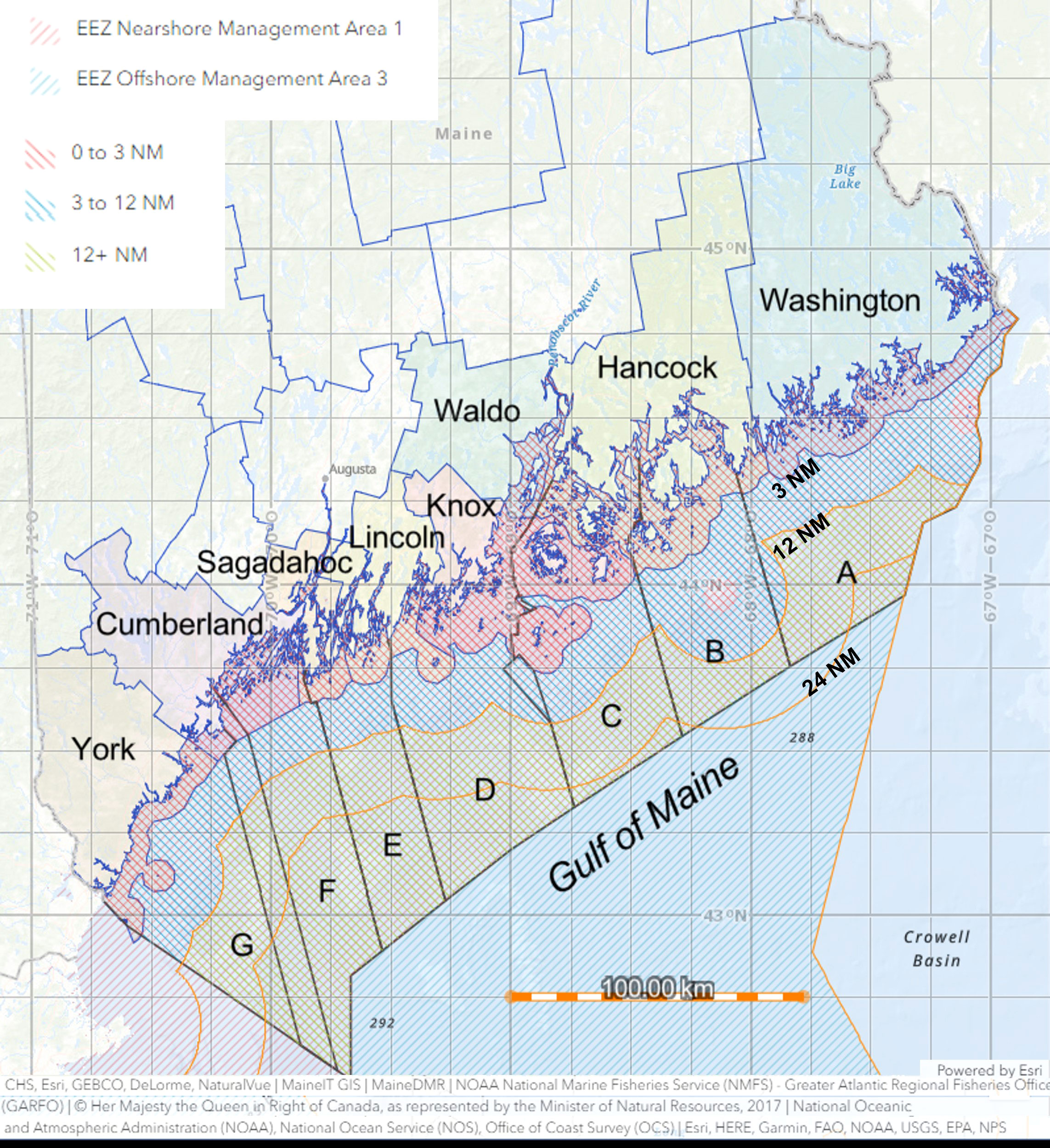
Figure 2 County and Zone (A-G) management boundaries of the Maine lobster fishery. Includes distance from shore lines (3 NM, 12 NM, and 24 NM), and federal management areas (near-shore area 1, near shore area 3).

Inshore boundaries for counties are not clearly defined, and zone and county lines do not match evenly (there are 8 counties and 7 lobster management zones). Furthermore, boundaries often overlap at ports of biological points of interest. Landings and active license data from the Maine DMR were used to develop analytical weights to convert county landings to zone landings (Table 1). Averaged proportional to averaged total yearly landings from 2004 to 2020 were used to determine what percent of county landings made up respective (nearby) zone landings. Geographical proximity and boundaries of counties and zones determined the direction and scale of analytical weights. Special attention and weights were given to key areas of interest, specifically Stonington Port (50% of zone C landings and licenses, majority producer of total state landings) and Vinalhaven (25% of zone C landings and licenses, second most producer of total state landings). Active licenses of counties and zones from the same data set were used to help correct analytical weights such that realized zone landings and licenses consist of approximately equal proportions of bordering county landings and licenses.

TABLE 1

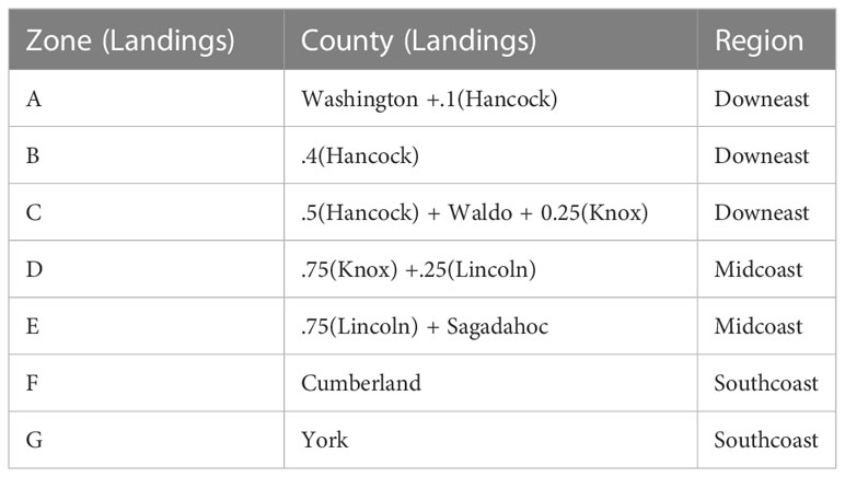
Table 1 Analytical weights for interpolating zone landings from proportions of county landings.

Interpolated zone-from-county landings were compared with realized zone landings using a paired t-test. Analytical weights were then used to interpolate past zone landings from past county landings (1978-2003). This is important for conducting hindcasting analysis of our models as historical county landings data goes back to 1964, but zone landings data only extends to 2004.

2.6 Landings-HSI model building and selection

We built a GAM to interpolate lobster fishery landings by zone from average HSI from the BE models. GAMs are favorable for this analysis as GAMs have predictive capacities of Generalized Linear Models to forecast and hindcast, but the functions are additive, and variables are smooth (Guisan et al., 2002). HSIs for each zone were averaged using an arithmetic mean for each season to obtain a single HSI value per zone per season for the years 2004-2018. A GAM was built on probable cause of predicting landings (observed) using spatially explicit, interpolated HSI, based on our best understanding of the seasonal and environmental nature of both lobster distributions and fishery behavior. A description of variables used can be found on Table 2. Spring and Fall HSI were always included as default variables. A GAM with all possible variables can be built as:

$$ln (Annual landing{s}_t) =s(Spring HS{I}_t)+s(Fall HS{I}_t)+Region+Zone+Regime + ϵ$$

TABLE 2

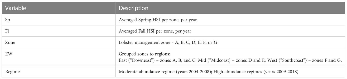
Table 2 Description of variables used in building the Landings-HSI GAM.

where $ln$is a natural log, $s$is a spline smoother, and $E$denotes an error term. VIF tests were conducted to each predicting variable to minimize multicollinearity. The GAM is able to predict landings as catchability for climate-driven habitat is implicit within HSI estimates. Making the model spatially explicit to zones allows us to connect HSI to fishery landings at a fine, management-specific scale. Due to our lack of seasonal landings data, we build the GAM to predict annual landings. Furthermore, the majority of landings are caught in the Summer (July-September) and Fall (October-December), while Winter (January-March) and Spring (April-June) seasons have been shown to be important for lobster reproduction and recruitment (Atlantic States Marine Fisheries Commission (ASMFC) American Lobster Stock Assessment Review Panel, 2020). In this, we assumed that the combined seasonal variability of lobster availability and landings is reflected in yearly landings.

Model results were evaluated using AIC, BIC, and Log Likelihood. Deviance explained and p-values were also considered for detailed comparisons. Models with the lowest AIC, BIC, and highest log-likelihood were chosen for further evaluation.

The GAM was used to predict landings using hindcasted historical HSI, and interpolated landings compared with historical landings data. Normalized root mean square error (NRMSE) and scatter index (SI) with observed historical data was used to evaluate model hindcasting performance. The GAM was then used to interpolate future landings based on forecasted HSI from the IPCC RCP 4.5 and 8.5 carbon emission climate scenarios. All model building and analysis was conducted in the statistical software R. A concept diagram of the methods for this study shows how data were analyzed to achieve the final results (Figure 3).

FIGURE 3

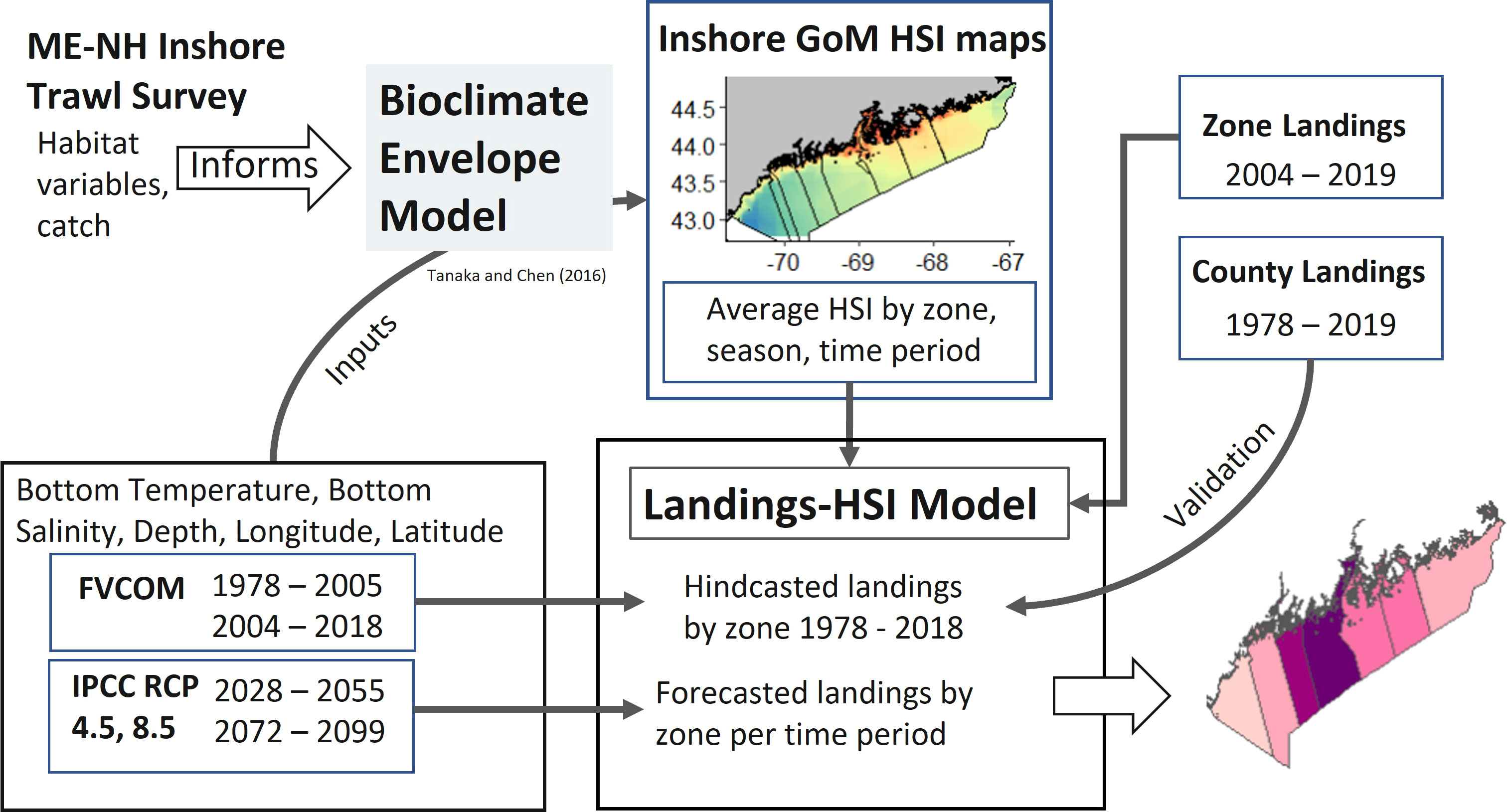
Figure 3 Concept diagram of methods of study.

3 Results

3.1 Suitability indices

There are seasonal differences in suitability for bottom temperature and bottom salinity between the spring and fall seasons (Figure 4). Spring optimum temperatures peak at 6.5 degrees Celsius (C), and are least favorable at 4.4 C. Spring temperatures range from 2.5 to 8.8 C. Fall optimum temperatures peak at 13 C, and are least favorable at 7.2 C. Fall temperatures range from 5.9 to 13.8 C. Spring suitable salinity ranges from 30.6 to 33.8 practical salinity units (psu), with a peak at 32.2 psu. Fall suitable salinity ranges from 31.5 to 34.6 psu, peaking at 32.4 psu. Spring and fall suitable depths share similar ranges from 14.6 to 201 meters (m). Suitability for optimum spring depth peaks at 47.5 m, while optimum fall depth plateaus from 34.7 to 45.7 m, and peaks at 65.8 m. The most suitable location for lobster in the inshore GoM in the spring is near a latitude of 44.15 and longitude of -68.48 degrees. The most suitable location in the fall is near a latitude of 43.92 and longitude of -69.45 degrees.

FIGURE 4

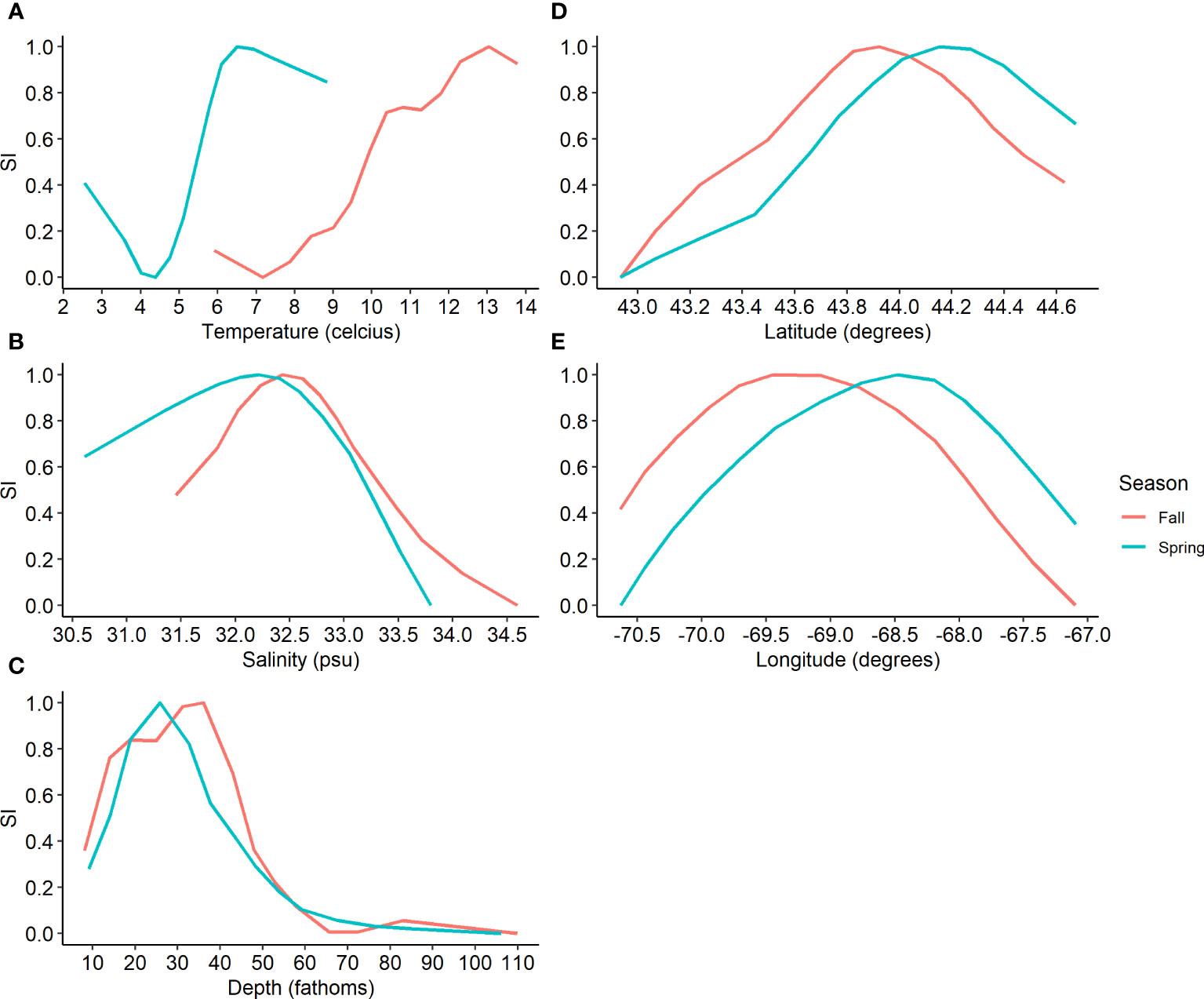
Figure 4 Smoothed suitability indices for spring (blue) and fall (red) bioclimate envelope models. SI’s range from 0 (least suitable) to 1 (most suitable). Habitat variables for SI’s are shown as follows: (A) Bottom temperature (Celsius); (B) Bottom salinity (psu); (C) Depth (fathoms); (D) Latitude (degrees); and (E) Longitude (degrees).

3.2 Habitat suitability indices

There appears to be seasonal differences in changes to HSI for the spring and fall over time. Currently and historically, the most suitable habitat for both spring and fall in all abundance regimes is along the coastal margin. From the low abundance regime to moderate abundance regime, HSI does not change much and even falls broadly in the spring and increases slightly in the Downeast region in the fall. However, from moderate to high abundance regimes HSI increases substantially throughout the entire inshore GoM, especially along the coast in Midocast and Downeast regions in the spring (Figure 5).

FIGURE 5

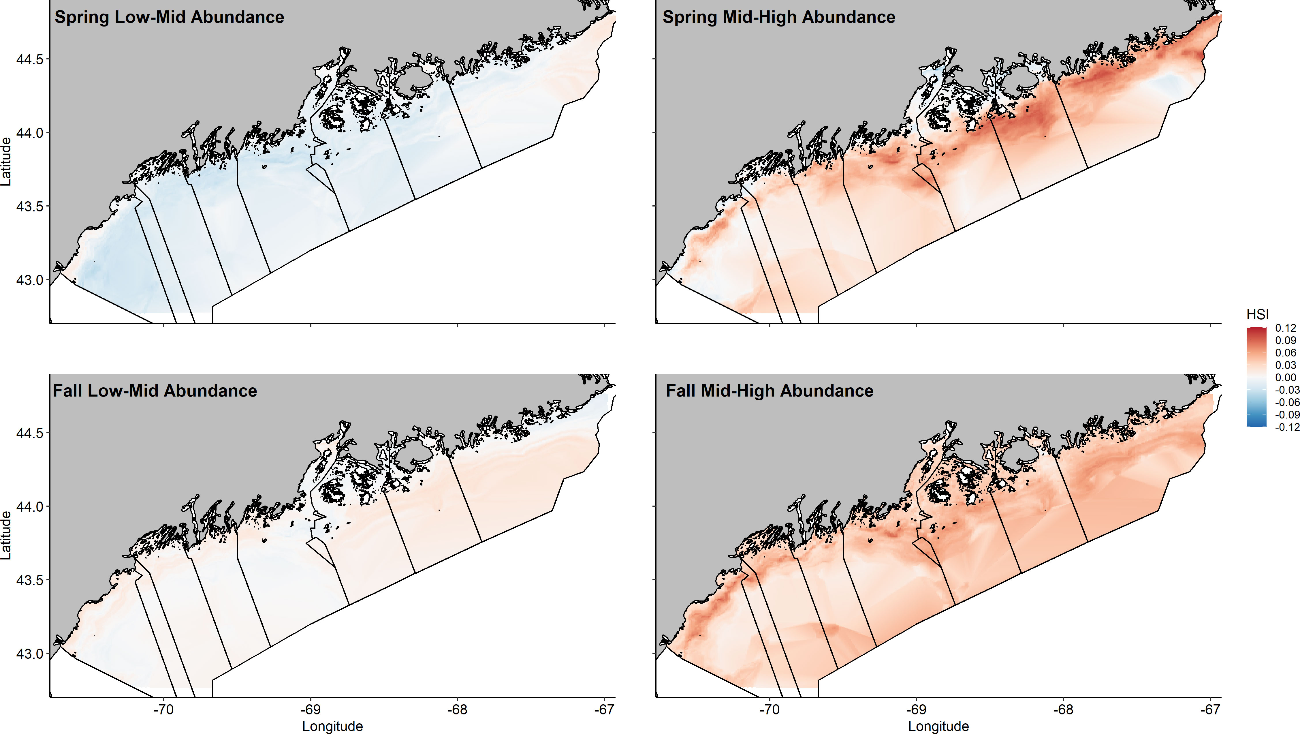
Figure 5 Change in interpolated habitat suitability index (HSI) from a low to moderate abundance regime (left column) and from a moderate to high abundance regime (right column) for the seasons spring (top row) and fall (bottom row). HSI values range from 0 (lowest) to 1 (highest). Lines depict Maine lobster management zones from A (northeast) to G (southwest).

There appears to be considerable seasonal differences in changes to HSI for near future (2028-2055) and far future (2072-2099) periods based on forecasted environmental parameters. Fall HSI for both RCP 4.5 and 8.5 scenarios is expected to increase for the entire study area. HSI is expected to increase more in the far future (2072-2099), and the most for RCP 8.5. Spring HSI however shows polarizing changes, with slight increases in HSI in the inshore Southcoast regions, but greater decreases in HSI for Midcoast, Downeast, and offshore Southcoast regions (Figures 6, 7).

FIGURE 6

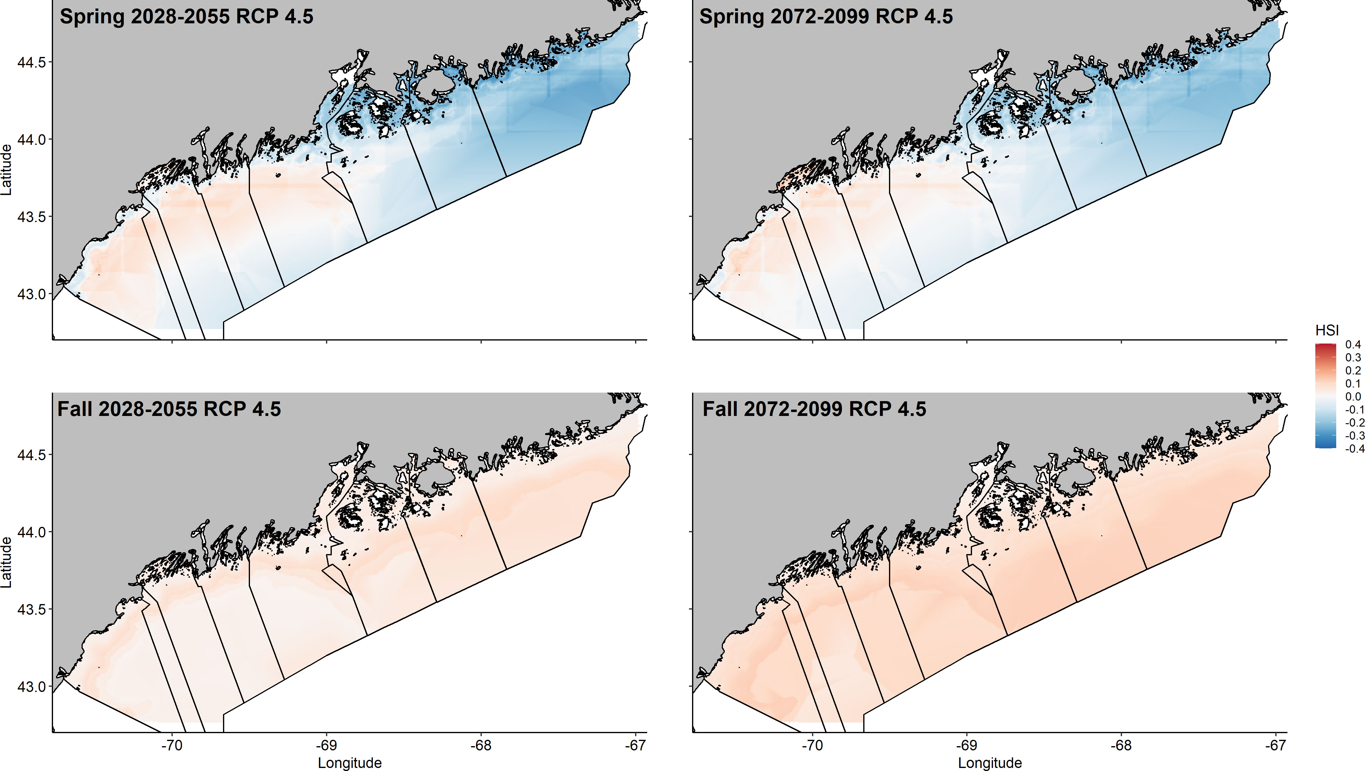
Figure 6 Change in interpolated habitat suitability index (HSI) from the baseline to the time periods 2028-2055 (left column) and 2072-2099 (right column) for the seasons spring (top row) and fall (bottom row) for RCO scenario 4.5. HSI values range from 0 (lowest) to 1 (highest). Lines depict Maine lobster management zones from A (northeast) to G (southwest).

FIGURE 7

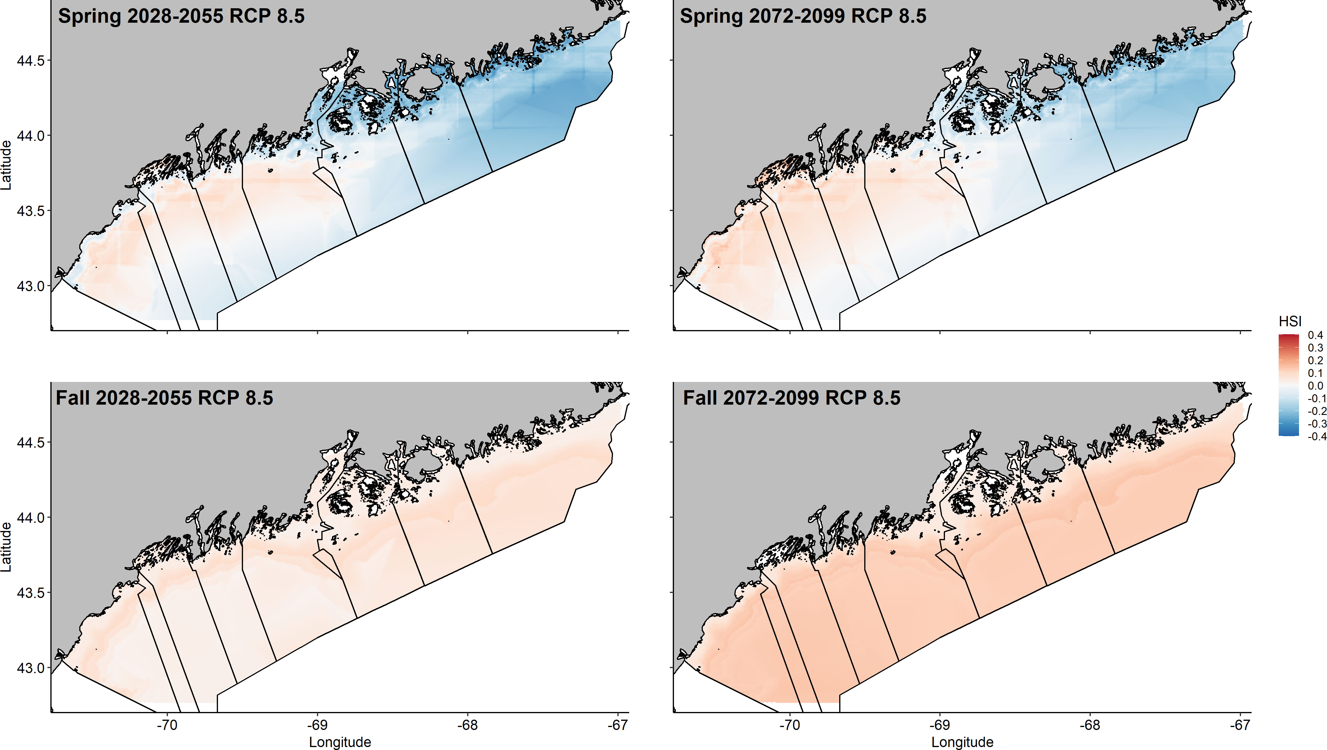
Figure 7 Change in interpolated habitat suitability index (HSI) from the baseline to the time periods 2028-2055 (left column) and 2072-2099 (right column) for the seasons spring (top row) and fall (bottom row) for RCO scenario 8.5. HSI values range from 0 (lowest) to 1 (highest). Lines depict Maine lobster management zones from A (northeast) to G (southwest).

3.3 Interpolated zone-county landings

Interpolated-from-county zone landings using analytical weights were compared to current county and zone landings from 2004 to 2020. T-test analysis shows no statistical difference between the interpolated and realized landings (p = 0.135) (Figure 8).

FIGURE 8

Figure 8 Total landings by zone over time for realized (left) and interpolated from county weights (middle) landings from 2004 to 2020. (right) One-to-one plot of realized and interpolated zone landings.

3.4 Model building and selections

Models were systematically built using available combinations of variables, and the best model was selected for further manipulation based on highest Log Likelihood, and lowest AIC and BIC values (Table 3). The variables Region and Zone were conflicting based on VIF testing and thus not included together for model building. The best model from the initial round of selection was:

TABLE 3

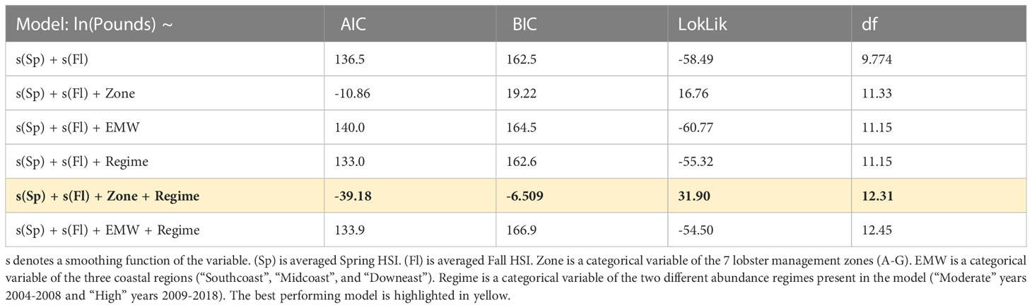
Table 3 AIC, BIC, Log Likelihood, and degrees freedom of initial GAM models were systematically built using all independent variables to predict the natural log of annual zone landings in pounds.

$\ln (Pounds)~ s(Spring HSI)+s(Fall HSI)+Zone+Regime$

The variable Region was used to spatially group HSI values to associated regional zones without overfitting the model (Table 4). After the second round of model selection, the final model used for analysis is:

TABLE 4

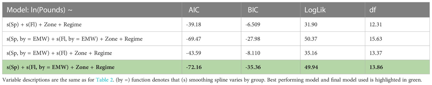
Table 4 AIC, BIC, Log Likelihood, and degrees freedom of secondary GAM models to predict natural log of annual zone landings in pounds.

$\ln (Pounds) ~ s(Spring HSI)+s(Fall HSI, by Region)+Zone+Regime$

The selected model performs well with majority statistically significant parametric coefficients and a deviance explained of 95%.

3.5 Landings-HSI GAM hindcasting

The model was used to predict landings using hindcasted environmental parameter from FVCOM to low abundance (1978-1995), moderate abundance (1996-2008), and high abundance (2009-2018) periods. Normalized root mean square error (NRMSE) and scatter index (SI) values were used to assess model hindcasting performance in order to correct for the high magnitude of error in RMSE values. The model performs terribly when hindcasted to low abundance periods. This is expected as this period exists outside of the periods for which the model is built (2004-2018). When hindcasted to a moderate abundance regime, the model performs considerably better, with a NRMSE of 20.5% and an SI of 44.1%. The model performs best for predicting to a high abundance regime with a NRMSE of 10.3% and SI of 18.3%. There appears to be clustering of landings based on zone, which suggests the model is able to capture spatial differences in landings along the coast (Figure 9).

FIGURE 9

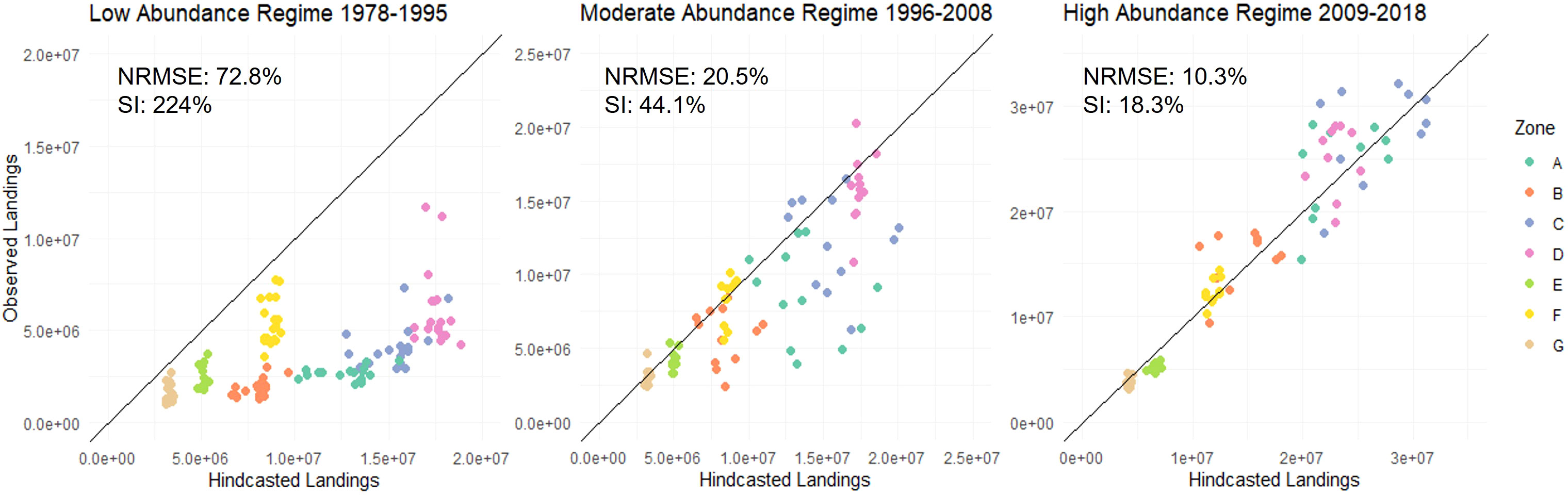
Figure 9 Observed vs hindcasted plots of landings (pounds) of the Landings-HSI GAM with hindcasted environmental data to the following different lobster abundance regimes: (left) Low abundance regime, (middle) Moderate abundance regimes, and (right) High abundance regime. NRMSE shows normalized root mean square error value. SI shows scatter index value. Different colors show groupings of different lobster management zones.

When hindcasted to a “post-lobster boom” period (moderate and high abundance regimes, 1996-2018), the model performs well with an overall NRMSE of 11.4% and an SI of 28.3%. The model is able to capture regional differences, with the greatest variability in Downeast regions at a NRMSE of 15.8% and an SI of 31.2% (Figure 10). The model does not appear to overpredict or underestimate landings for all zones. Hindcasting analysis gives confidence in the model’s ability to predict for landings given environmental parameters if in the same moderate or high abundance regimes.

FIGURE 10

Figure 10 Observed vs hindcasted plot of landings (pounds) of the Landings-HSI GAM with hindcasted environmental data to post lobster boom period (Moderate and High abundance regimes 1996-2018) (left). Different colors show groupings of different lobster management zones. Normalized root mean square error (NRMSE) and Scattter Index (SI) values of different coastal regions matched by corresponding zones (right).

3.6 Landings-HSI GAM forecasting

The model was used to predict landings using forecasted IPCC environmental parameters for the near future and far future periods, for both RCP 4.5 and 8.5 scenarios, and for assuming if lobster abundances stay in a high regime or fall back down to a moderate regime (Figure 11). It appears that from the previous period (1996-2008) to current period (2009-2018), landings for all zones increased, most notably in Zones A, B, C, D, and F. From the current period (2009-2018) to the near future (2028-2055), landings for Zones A, B, C, and D are expected to decrease, F and G, stay relatively similar, and E to increase. For the far future (2072-2099), landings for Zone D are expected to continue to decrease, but landings for Zones A, B, and C are expected to rise again to similar levels of current landings. Landings for Zones E, F, and G are expected to decrease slightly in the far future. There appears to be little difference in changes in landings between RCP scenarios until the far future for Zones A, B, and C, where RCP scenario 8.5 are expected to show greater increases in landings. All zone landings will decrease if lobster abundances fall back to a moderate abundance regime (dashed line). This shift in decreases in landings is proportionally consistent among all zones, as there is no difference between high or moderate abundance regimes to changes in the percent of total landings. When considering proportional (percent) landings for the entire coast, landings for Zone D constantly decrease over time where as landings for Zone C will increase. Proportional landings for all other zones stay relatively consistent, which suggests that despite decreases or increases in total landings, the spatial distribution of landings is less affected.

FIGURE 11

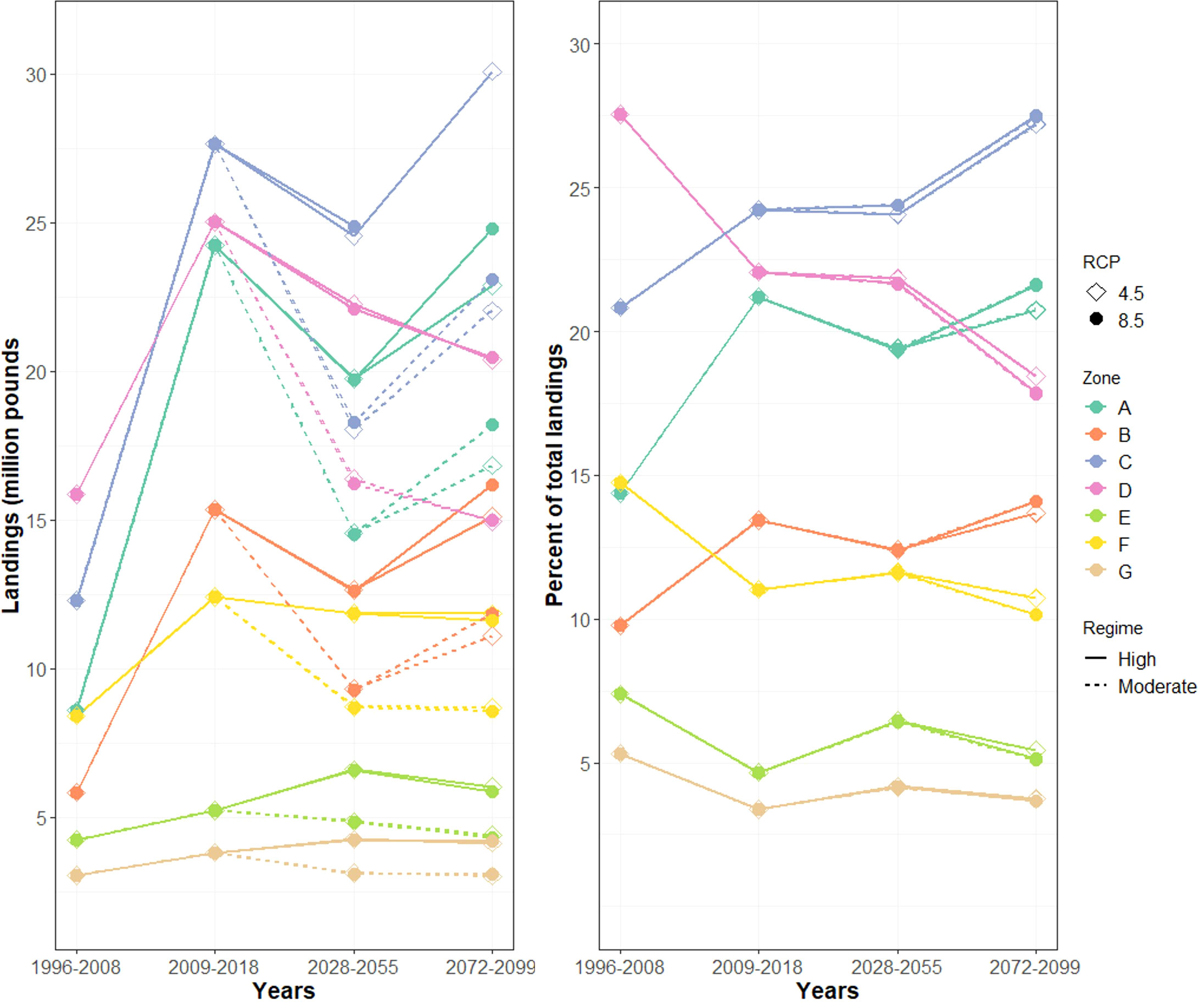
Figure 11 Left: Total interpolated landings from the Landings-HSI model for historical (1978-2005), baseline (2004-2017), and forecasted (2028-2055; 2072-2099) time periods and RCP 4.5 and 8.5 scenarios. Right: Percent of total interpolated landings from the Landings-HSI model for historical (1978-2005), baseline (2004-2017), and forecasted (2028-2055; 2072-2099) time periods and RCP 4.5 and 8.5 scenarios.

4 Discussion

The model’s ability to differentiate between a moderate and high abundance regime allows for an analysis of changes in the distribution of future lobster landings given different climate and abundance regime scenarios. Lobster abundances have historically increased significantly from a low abundance regime to a moderate abundance regime, dubbed the “lobster boom.” Unfortunately, the model cannot hindcast reliably to a low abundance regime before 1996. However, seasonal HSI does not change drastically between low and moderate abundance regimes. This suggests that the lobster boom and initial increase in lobster abundances may be due to other factors beyond just climate-driven habitat, such as a conservation focused management and a decrease in predators (Zhang and Chen, 2007; Zhang et al., 2012; Mazur et al., 2019). The model can, however, hindcast much more reliably to a moderate (1996-2008) and high (2009-2018) abundance regime. Furthermore, seasonal HSI increased drastically more from a moderate to high abundance regime. This suggests that the most recent shift in lobster abundances is more influenced by climate-driven habitat. This is further supported by the collapse of the Atlantic cod fishery in 1993 which vastly reduced predation (Pershing et al., 2015; Meng et al., 2016) and the fact that recruitment and conservation focused management have been long established in the fishery by this point in time (Atlantic States Marine Fisheries Commission (ASMFC) American Lobster Stock Assessment Review Panel, 2020).

Despite expected decreases in total landings, lobster landings in all zones are still likely to be higher than historical levels (Goode et al., 2019). It is interesting to note the differences in patterns of changes of proportional landings between regions. Downeast (Zones A, B, and C) landings are expected to decrease, then increase again to current levels of landings. Midcoast (Zones D and E) appear to split in different directions of change, with Zone D landings decreasing consistently while Zone E landings increases, then decreases. Southcoast (Zones F and G) landings seem less affected by changes in climate-driven habitat. It appears that the initial decrease in landings for the Downeast region in the near future may be due to the decreases in spring HSI for the same area. The following increase in landings for the far future in Downeast zones may be then due to the much higher increase in fall HSI for the far future. This is further supported by the greater increase in landings for RCP 8.5 scenarios which also see greater increases in HSI for far future Downeast zones. This suggests that seasonal climate may play a greater role in total lobster landings than previously thought.

These findings are somewhat inconsistent with previous studies that suggest a northeast shift of fishing effort and lobster habitat distributions (Tanaka and Chen, 2016; Boenish and Chen, 2017; Rheuban et al., 2017). However, these studies do not differentiate between seasons, zones, or inshore and offshore regions. Similar works that examine the seasonal habitat suitability of American lobster for a much larger area including the inshore GoM suggest an inverse seasonal relationship from this study where spring habitat suitability increases more and fall habitat suitability does not (Mazur et al., 2020; Tanaka et al., 2020). However, recent work with bioclimate models in the GoM shows that including non-stationarity differences between localized regions, especially between eastern and western GoM, improved HSI distribution estimates (Behan et al., 2021; Behan et al., 2022). The fine spatial scale of the inshore and zone focus of our study may allow our model to capture details about inshore spatial processes absent from models with larger study areas and on coarse spatial scales. Additionally, the inclusion of seasonality may highlight important trends that are absent on a yearly scale. The addition of offshore environment data cannot be directly compared to historical near-shore fishery landings data and is beyond the scope of this study. These findings are more consistent with recent work that suggests a decrease in favorable lobster conditions in inshore Downeast regions (Zones A, B, and C), but an expansion of favorable conditions more offshore in the same regions (Goode et al., 2019; Hodgdon et al., 2021).The results of our study highlight the importance of considering a fine spatial and temporal scale in studying the impacts of climate changes on fisheries.

There are multiple factors related to climate that may influence the change in future landings for the inshore GoM area. Lobster fishery landings are known to be related to juvenile lobster abundance and lobster larvae settlement in the past (Steneck and Wilson, 2001; Goode et al., 2019);. Bottom temperature and salinity have a significant influence on lobster reproduction, larval settlement, and growth (Incze and Wahle, 1991; Steneck and Wilson, 2001; Oppenheim et al., 2019). Rising temperatures have been shown to increase growth and may increase the dispersal of lobster larvae, but reduce survival (Waller et al., 2016; Quinn et al., 2022);. Particle modeling of lobster larvae shows that the distribution of larvae is highly dependent on the Gulf of Maine Coastal Current (GMCC), and recruitment seeds directly to regions southwest along the coast (Xue et al., 2007). Assuming the relationship between lobster landings and larvae settlement stays true, lobster fishery landings may shift toward deeper and offshore waters as suitable habitat for larvae shift in a similar direction (Goode et al., 2019; Oppenheim et al., 2019). This phenomenon is already observed in southern New England, where lobster larvae settlement, distribution, and commercial landings have all shifted offshore as inshore habitats become too warm (Casey et al., 2022). Another cause may be that phenology of local lobster migrations are shifting earlier and lasting longer (Mills et al., 2013; Le Bris et al., 2018; Staudinger et al., 2019). Because lobster recruitment is highly seasonal, changes in climate in either spring or fall may affect reproductive success of lobsters (Oppenheim et al., 2019). There have been some notable changes in the hydrographic, biogeochemical, and acidity of the GoM since 1998 including a decline in phytoplankton primary production (Balch et al., 2022). This reinforces the difference in landings between current and previous abundance regimes. Seasonal variability and changes to currents are inherent within forecasted environmental parameters, which allows our model to capture some effects of climate change in a complex multidimensional environmental scale. However, further change in oceanographic conditions is likely to affect fishery landings.

These findings have clear implications for the long-term management of the Maine lobster fishery. As a highly localized fishery, understanding the distribution and projection of landings along the coast can inform policies that strengthen existing infrastructure to optimize fishery productivity. Additionally, these findings can help inform policies to build economic resilience in areas with projected decreased landings, which can take forms in alternative fisheries or sources of income, mobility, exit strategies, or greater fishery capacity. As the Maine lobster fishery is highly heterogenous, understanding the differences in behavior and response of the fishery to climate change can provide a much greater insight to the distributional and relative impacts of climate change to the fishery and dependent coastal communities (Le Bris et al., 2018; Greenan et al., 2019; McClenachan et al., 2020).

It is important to recognize several limitations in our model. Firstly, the survey used may not be able to capture the full habitat range of American lobster as lobsters are known to favor complex, rocky habitat which is often not properly sampled by trawling, and thus may have bias toward soft bottom habitat (Lawton and Lavalli, 1995). However, we did not have access to unbiased survey data or habitat and abundance data over rocky substrate. Additionally, the substrate data available was on a far coarser scale and would not be informative to our fine-scale spatial analysis. As such, we do not include substrate in our model and analysis, but is noted that substrate can play an important role in lobster habitat. Future studies should utilize a finer scale substrate dataset, or incorporate varying suvey data if available. Secondly, despite our fine spatial scale, our temporal scale is lacking. Although we assume yearly landings reflect seasonal biological processes, modeling seasonal landings dynamics may improve our understanding of the effects of habitat on fishery landings. Additionally, our assumptions and findings are limited to near-shore areas only and may not reflect far offshore processes such as in Tanaka et al. (2020) and Mazur et al. (2020). While the importance of non-staionarity effects and the near-shore nature of the has been etablshed, this analysis cannot extend to areas beyond the spatial boundary of this study. As such, we highlight a need for similar, updated fine scale analysis of offshore ecological change and offshore fishery landings. Thirdly, we implicitly assume that the relationship between habitat suitability and fishery landings, and thus fishery behavior, is stationary. However, realized fishery behavior (fishing effort, fishing mortality, bait input) are subject to socio-economic, political, and climate changes and can have far reaching community impacts (Martin, 2006). Thus, we highlight the need for a more in-depth examination of fishery behavior data to fully understand the socio-economic implications for climate change effects in the GoM.

This study serves as a case study example for connecting fishery processes to environmental parameters through the use of a bioclimate envelope model and fishery landings. This is important for understanding the direct effects of climate change on fisheries. We emphasize the fine-scale spatial nature of our study and the resulting details which are often lost in many ocean habitat or fishery models. A similar concept can be applied to other fisheries and other habitats, with consideration for important key variables in other systems. While most other fishery models use exclusively fishery independent data, we use this study to highlight a combination of fishery data and fishery independent survey data may provide important insights to connecting climate science to fishery processes. Expanding on models such as this may allow for the linking of ecological models with fishery behavior data (fishing effort, input, and strategies), which may serve as a basis for a bio-economic model to examine distributional effects of climate change at both an ecological and human dimension. This can further help fishery dependent coastal communities in favor of long-term sustainability through adaptation and resilience strategies to climate change in the fishery.

Data availability statement

Publicly available datasets were analyzed in this study. This data can be found here: Maine Department of Marine Resources; https://www.maine.gov/dmr/fisheries/commercial/landings-program/historical-data – Landings Data; https://www.maine.gov/dmr/science/fisheries-monitoring-assessment/maine-new-hampshire-inshore-trawl-survey – Trawl Survey Data University of Massachusetts Dartmouth School for Marine Science and Technology; http://fvcom.smast.umassd.edu/fvcom/– FVCOM environmental data IPCC Climate Data – NOAA Climate Change Web Portal; https://psl.noaa.gov/ipcc/ocn/.

Author contributions

JK: Methodology, Software, Formal analysis, Investigation, Data Creation, Writing – original Draft, Visualization. CH: Methodology, Software, Writing – Review & Editing. KE: Writing – Review & Editing, Funding acquisition. YC: Conceptualization, Supervision, Project administration, Writing – Review & Editing. All authors contributed to the article and approved the submitted version.

Funding

This study is funded by the Coastal and Ocean Climate Applications (COCA) grant #2741085 from the National Oceanic and Atmospheric Administration (NOAA) and the USDA National Institute of Food and Agriculture under Hatch projects # ME022202.

Acknowledgments

The authors would like to thank the members and alumni of the Chen lab at the University of Maine and Stony Brook University for their feedback and input for this manuscript. In particular, we thank Jamie Behan for her extensive work on data extrapolation and model building code.In addition, we would like to thank the Maine DMR for providing the necessary data and their collaboration on this project. We also thank the Chen lab at the University of Massachussetrs, Dartmouth for providing FVCOM environmental data. Finally, we thank Bori B. Cha for his continual support of the lead author.

Conflict of interest

The authors declare that the research was conducted in the absence of any commercial or financial relationships that could be construed as a potential conflict of interest.

Publisher’s note

All claims expressed in this article are solely those of the authors and do not necessarily represent those of their affiliated organizations, or those of the publisher, the editors and the reviewers. Any product that may be evaluated in this article, or claim that may be made by its manufacturer, is not guaranteed or endorsed by the publisher.

Supplementary material

The Supplementary Material for this article can be found online at: https://www.frontiersin.org/articles/10.3389/fmars.2023.1171269/full#supplementary-material

References

Acheson J. M. (1988). The lobster gangs of Maine (Hanover, NH: The New England University Press).

Google Scholar

Acheson J., Stockwell. T., Wilson J. A. (2000). “Evolution of the Maine lobster Co-management law. ” Maine Policy Rev. Available at: 9.2, : 52–: 562. https://digitalcommons.library.umaine.edu/mpr/vol9/iss2/7

Google Scholar

Akima H., Gebhardt A. (2016). “Akima: interpolation of irregularly and regularly spaced data,” in R package version 0.6-2. https://cran.rproject.org/web/packages/akima/akima.pdf

Google Scholar

Atlantic States Marine Fisheries Commission (ASMFC) American Lobster Stock Assessment Review Panel (2020). American Lobster benchmark stock assessment and peer review report (Massachusetts: Woods Hole), 506.

Google Scholar

Balch W. M., Drapeau D. T., Bowler B. C., Record N. R., Bates N. R., Pinkham S., et al. (2022). Changing hydrographic, biogeochemical, and acidification properties in the gulf of Maine as measured by the gulf of Maine north Atlantic time series, GNATS, between 1998 and 2018. J. Geophys. Res.: Biogeosci. 127, e2022JG006790. doi: 10.1029/2022JG006790

PubMed Abstract | CrossRef Full Text | Google Scholar

Behan J. T., Hodgdon C. T., Chen Y. (2022). Scale-dependent assumptions influence habitat suitability estimates for the American lobster (Homarus americanus): implications for a changing gulf of Maine. Ecol. Model. 470. doi: 10.1016/j.ecolmodel.2022.110030

CrossRef Full Text | Google Scholar

Behan J. T., Li B., Chen Y. (2021). Examining scale dependent environmental effects on American lobster (Homarus americanus) spatial distribution in a changing gulf of Maine. Front. Mar. Sci. 8. doi: 10.3389/fmars.2021.680541

CrossRef Full Text | Google Scholar

Boenish R., Chen Y. (2017). Spatiotemporal dynamics of effective fishing effort in the American lobster ( homarus americanus ) fishery along the coast of Maine Vol. 199 (USA: Fisheries Research). doi: 10.1016/j.fishres.2017.11.001

CrossRef Full Text | Google Scholar

Brown S. K., Buja K. R., Steven H. Jury S. H., Monaco M. E., Banner A. (2000). Habitat suitability index models for eight fish and invertebrate species in casco and sheepscot bays, Maine. North Am. J. Fisheries Manage. 20, 408–435. doi: 10.1577/1548-8675(2000)0202.3.CO;2

CrossRef Full Text | Google Scholar

Casey F., Churchill J. H., Cowles G. W., Pugh T. L., Wahle R. A., Stokesbury K. D. E., et al. (2022). The impact of ocean warming on juvenile American lobster recruitment off southeastern Massachusetts. Fisheries Oceanog. 1–16. doi: 10.1111/fog.12625

CrossRef Full Text | Google Scholar

Chen Y., Wilson C., Scheirer K., Couture D., Wilson J. (2005). Spatial dynamics of the lobster fishery and oil spills in the gulf of Maine, a risk analysis of oil spills on the lobster fishery (MOSAC/DEP/Sea Grant Report).

Google Scholar

Cheung W. W. L., Jones M. C., Reygondeau G., Stock C. A., Lam V. W. Y., Frolicher T. L. (2016). Structural uncertainty in projecting global fisheries catches under climate change (Ecological Modelling). doi: 10.1016/j.ecolmodel.2015.12.2018

CrossRef Full Text | Google Scholar

Cushing D. H. (1982). Climate and fisheries (NY. Academic Press Inc: New York).

Google Scholar

Donihue M. (2018). Lobsters to dollars: the economic impact of the lobster distribution supply chain in Maine (Waterville , ME: Colby College).

Google Scholar

Franklin J. (2010). Mapping species distributions: spatial inference and prediction. Eds. Usher M., Saunders D., Peet R., Dobson A. (New York, NY: Cambridge University Press).

Google Scholar

Goode A. G., Brady D. C., Steneck R. S., Wahle R. A. (2019). The brighter side of climate change: how local oceanography amplified a lobster boom in the gulf of Maine. Glob Change Biol. 25, 3906–3917. doi: 10.1111/gcb.14778

CrossRef Full Text | Google Scholar

Grabowski J. H., Clesceri E. J., Baukus A., Gaudette J., Weber M., Yund P. O. (2010). Use of herring bait to farm lobsters in the gulf of Maine. PloS One 5, e10188. doi: 10.1371/journal.pone.0010188

CrossRef Full Text | Google Scholar

Greenan B. J. W., Shackell N. L., Ferguson K., Greyson P., Cogswell A., Brickman D., et al. (2019). Climate change vulnerability of American lobster fishing communities in Atlantic Canada. Front. Mar. Sci. 6. doi: 10.3389/fmars.2019.00579

CrossRef Full Text | Google Scholar

Guisan A., Edwards T. C., Hastie T. (2002). Generalized linear and generalized additive models in studies of species distributions: setting the scene. Ecol. Modell. 157, 89–100. doi: 10.1016/S0304-3800(02)00204-1

CrossRef Full Text | Google Scholar

Gulf of Maine Research Institute (2008) Taking the pulse of the lobster industry : a socioeconomic survey of new England lobster fishermen. Available at: www.gmri.org/upload/files/gmri_lobster_report_lores.pdf.

Google Scholar

Hijmans R. J., van Etten J. (2012). “Raster: geographic analysis and modeling with raster data,” in R package version 2.0-12. Available at: http://CRAN.R-project.org/package=raster.

Google Scholar

Hodgdon C. T., Mazur M. D., Friedland K. D., Willse N., Chen Y. (2021). Consequences of model assumptions when projecting habitat suitability: a caution of forecasting under uncertainties. ICES J. Mar. Sci. 78, 2092–2108. doi: 10.1093/icesjms/fsab101

CrossRef Full Text | Google Scholar

Incze L. S., Wahle R. A. (1991). Recruitment from pelagic to early benthic phase in lobsters, Homarus americanus. Mar. Ecol. Prog. Series 79, 77–97.

Google Scholar

Jewett L., Romanou A. (2017). Ocean acidification and other ocean changes. in climate science special report: fourth national climate assessment, volume I. Eds. Wuebbles D. J., Fahey D. W., Hibbard K. A., Dokken D. J., Stewart B. C., Maycock T. K. (U.S. Global Change Research Program), 364–392. doi: 10.7930/J0QV3JQB

CrossRef Full Text | Google Scholar

Kleisner K. M., Fogarty M. J., McGee. S., Hare J. A., Moret S., Perretti C. T., et al. (2017). Marine species distribution shifts on the u. s. northeast continental shelf under continued ocean warming. Prog. Oceanog. 153, 24–36. doi: 10.1016/j.pocean.2017.04.001

CrossRef Full Text | Google Scholar

Lawton P., Lavalli K. L. (1995). “Chapter 4 - postlarval, juvenile, adolescent, and adult ecology,” in Biology of the lobster (New York, NY: Academic Press), 47–88. doi: 10.1016/B978-012247570-2/50026-8

CrossRef Full Text | Google Scholar

Le Bris A., Mills K. E., Wahle R. A., Chen Y., Alexander M. A., Allyn A. J., et al. (2018). Climate vulnerability and resilience in the most valuable north American fishery. PNAS 115 (8), 1831–1836. doi: 10.1073/pnas.1711122115

CrossRef Full Text | Google Scholar

Lehodey P., Alheit J., Barange M., Baumgartner T., Beaugrand G., Drinkwater K., et al. (2006). Climate variability, fish, and fisheries. J. Climate 19 (20), 5009–5030. doi: 10.1175/JCLI3898.1

CrossRef Full Text | Google Scholar

Li B., Tanaka K., Chen Y., Brady D. C., Thomas A. C. (2017). Assessing the quality of bottom water temperatures from the finite-volume community ocean model (FVCOM) in the Northwest Atlantic shelf region. J. Mar. Syst 173, 21–30. doi: 10.1016/j.jmarsys.2017.04.001

CrossRef Full Text | Google Scholar

Maine Lobstermen’s Community Alliance (MLCA) (2021) All about lobster: 2.3: lobstering season and licensing. Available at: https://mlcalliance.org/all-about-lobster/lobster-2-3-season-and-licensing/.

Google Scholar

Maine Department of Marine Resources (MEDMR) (2020). Historical Maine Fisheries Landings Data [online]. Maine Department Mar. Resour. https://bit.ly/2rV0yzf.

Google Scholar

Martin S. (2006). “The impact of ‘Community' on fisheries management in the U.S. Northeast." Geoforum 37 (2), 169–184. doi: 10.1016/j.geoforum.2005.05.004

CrossRef Full Text | Google Scholar

Mazur M. D., Friedland K. D., McManus M. C., Goode A. G. (2020). Dynamic changes in American lobster suitable habitat distribution on the northeast U.S. shelf linked to oceanographic conditions. Fish Oceanogr 29, 349–365. doi: 10.1111/fog.12476

CrossRef Full Text | Google Scholar

Mazur M. D., Li B., Chang J., Chen. Y. (2019). Contributions of a conservation measure that protects the spawning stock to drastic increases in the gulf of Maine American lobster fishery. Mar. Ecol. Prog. Ser. 631, 127–139. doi: 10.3354/meps13141

CrossRef Full Text | Google Scholar

McClenachan L., Scyphers S., Grabowski J. K. (2020). Views from the dock: warming waters, adaptation, and the future of maine’s lobster fishery. Ambio 49, 144–155. doi: 10.1007/s13280-019-01156-3

CrossRef Full Text | Google Scholar

Meng K. C., Oremus K. L., Gaines S. D. (2016). New England cod collapse and the climate. PloS One 11 (7), e0158487. doi: 10.1371/journal.pone.0158487

CrossRef Full Text | Google Scholar

Mills K., Pershing A. J., Brown C. J., Chen Y., Chiang F., Holland D. S., et al. (2013). Fisheries management in a changing climate: lessons from the 2012 ocean heat wave in the Northwest Atlantic. Oceanography 26 (2), 191–195. doi: 10.5670/oceanog.2013.27

CrossRef Full Text | Google Scholar

Morris L., Ball D. (2006). Habitat suitability modelling of economically important fish species with commercial fisheries data. e ICES J. Mar. Sci. 63, 1590e1603. doi: 10.1016/j.icesjms.2006.06.008

CrossRef Full Text | Google Scholar

NOAA, Fisheries (2013). “Fish stock assessment 101 series: part 3–ecosystem factors and assessments,” in Population assessments: fish stocks (NOAA). Available at: https://www.fisheries.noaa.gov/topic/population-assessments.

Google Scholar

Oppenheim N. G., Wahle R. A., Brady D. C., Goode A. G., Pershing A. J. (2019). The cresting wave: larval settlement and ocean temperatures predict change in the American lobster harvest. Ecol. Appl. 29 (8), e02006. doi: 10.1002/eap.2006

CrossRef Full Text | Google Scholar

Pershing A. J., Alexander M. A., Hernandez C. A., Kerr L. A., Le Bris A., Mills K. E., et al. (2015). Slow adaptation in the face of rapid warming leads to collapse of the gulf of Maine cod fishery. Science 250, Issue 6262, 809–812. doi: 10.1126/science.aac9819

CrossRef Full Text | Google Scholar

Quinn B. K., Chasse J., Rochette R. (2022). Impact of the use of different temperature-dependent larval development functions on estimates of potential large-scale connectivity of American lobster. Fisheries Oceanog. 31, 554–569. doi: 10.1111/fog.12606

CrossRef Full Text | Google Scholar

Rheuban J. E., Kavanaugh M. T., Doney S. C. (2017). Implications of future northwest Atlantic bottom temperatures on the American lobster (Homarus americanus) fishery. J. Geophys. Res.: Oceans 122, 9387–9398. doi: 10.1002/2017JC012949

CrossRef Full Text | Google Scholar

Rowden A. A., Anderson O. F., Georgian S. E., Bowden D. A., Clark M. R., Pallentin A., et al. (2017). High-resolution habitat suitability models for the conservation and management of vulnerable marine ecosystems on the Louisville seamount chain, south pacific ocean. Front. Mar. Sci. 4. doi: 10.3389/fmars.2017.00335

CrossRef Full Text | Google Scholar

Schuetz J., Mills K., Allyn A., Stamieszkin K., Bris A., Pershing A. (2019). Complex patterns of temperature sensitivity, not ecological traits, dictate diverse species responses to climate change. Ecography 42 (1), 111–124. doi: 10.1111/ecog.03823

CrossRef Full Text | Google Scholar

Sherman S., Stepanek K., Sowles J. (2005). Maine–New Hampshire inshore groundfish trawl survey: procedures and protocols. W. Boothbay Harbor 42.

Google Scholar

Staudinger M. D., Mills K. E., Stamieszkin K., Record N.R., Hudak C.A., Allyn A., et al. (2019). It's about time: a synthesis of changing phenology in the gulf of Maine ecosystem. Fish Oceanogr. 28, 532–566. doi: 10.1111/fog.12429

CrossRef Full Text | Google Scholar

Steneck R. S., Wilson C. J. (2001). Large-Scale and long-term, spatial and temporal patterns in demography and landings of the American lobster, homarus americanus, in Maine. Marine and Freshwater Research. 52 (8), 1303–1319. doi: 10.1071/MF01173

CrossRef Full Text | Google Scholar

Tanaka K. R., Cao J., Shank B. V., Truesdell S. B., Mazur M. D., Xu L., et al. (2019). A model-based approach to incorporate environmental variability into assessment of a commercial fishery: a case study with the American lobster fishery in the gulf of Maine and georges bank. – ICES J. Mar. Sci. 76, 884–896. doi: 10.1093/icesjms/fsz024

CrossRef Full Text | Google Scholar

Tanaka K. R., Chen Y. (2016). Modelling spatiotemporal variability of the bioclimate envelope homarus americanus in the coastal waters of Maine and new Hampshire. Fisheries Res 177, 137–152. doi: 10.1016/j.fishres.2016.01.010

CrossRef Full Text | Google Scholar

Tanaka K. R., Torre M. P., Saba V. S., Stock C. A., Chen Y. (2020). An ensemble high-resolution projection of changes in the future habitat of American lobster and sea scallop in the northeast US continental shelf. Divers. Distrib 26, 987–1001. doi: 10.1111/ddi.13069

CrossRef Full Text | Google Scholar

Waller J. (2016). “Linking rising pCO2 and temperature to the larval development, physiology and gene expression of the American lobster (Homarus americanus)" (Electronic Theses and Dissertations), 2527. Available at: https://digitalcommons.library.umaine.edu/etd/2527.

Google Scholar

Xue Y., Guan L., Tanaka K., Zengguang L., Chen Y., Ren Y. (2017). Evaluating effets of rescaling and weighting data on habitat suitability odeling. Fisheries Res. 188 (2017), 84–94. doi: 10.1016/j.fishres.2016.12.001

CrossRef Full Text | Google Scholar

Xue H., Incze L., Xu D., Wolff N., Pettigrew N. (2007). Connectivity of lobster populations in the coastal gulf of maine. part I: circulation and larval transport potential. Ecol. Modelling. 210 (2008), 193–211. doi: 10.1016/j.ecolmodel.2007.07.024

CrossRef Full Text | Google Scholar

Zhang Y., Chen Y. (2007). Modeling and evaluating ecosystem in 1980s and 1990s for American lobster (Homarus americanus) in the gulf of Maine. Ecol. Modeling 203, 475–489. doi: 10.1016/j.ecolmodel.2006.12.019

CrossRef Full Text | Google Scholar

Zhang Y., Li Y., Chen Y. (2012). Modeling the dynamics of ecosystem for the American lobster in the gulf of Maine. Aquat. Ecol. 46, 451–464. doi: 10.1007/s10452-012-9414-z

CrossRef Full Text | Google Scholar