Oceanic and ecological response to native Typhoons Cempaka and Lupit (2021) along the northern South China Sea continental shelf: comparison and evaluation of global and regional Operational Oceanography Forecasting Systems

1 Introduction

The northern South China Sea (SCS) continental shelf is located next to the Guangdong Province and includes the Guangdong–Hongkong–Macau Greater Bay Area waters with a depth of 0–200 m. It covers numerous islands, winding shorelines, and a complex topography (Figure 1A). Its dynamic processes are not only forced by the East Asian Monsoon (Wyrtki, 1961; Qu, 2000) but also significantly affected by the Kuroshio intrusion from the Luzon Strait (Farris and Wimbush, 1996; Nan et al., 2013). In addition, several estuaries along the northern SCS shelf dramatically affect the regional marine systems through runoff discharge. The most representative is the Pearl River Estuary (PRE, Figure 1A), the second-largest river in China and the 13th-largest river in the world, in terms of runoff discharge. The annual average runoff discharge of the PRE is 10,524 m³ s⁻¹, of which 80% occurs during April–September with a maximum in July, making an important contribution to the physical and ecological environment in and near the PRE (Zhao, 1990).

FIGURE 1

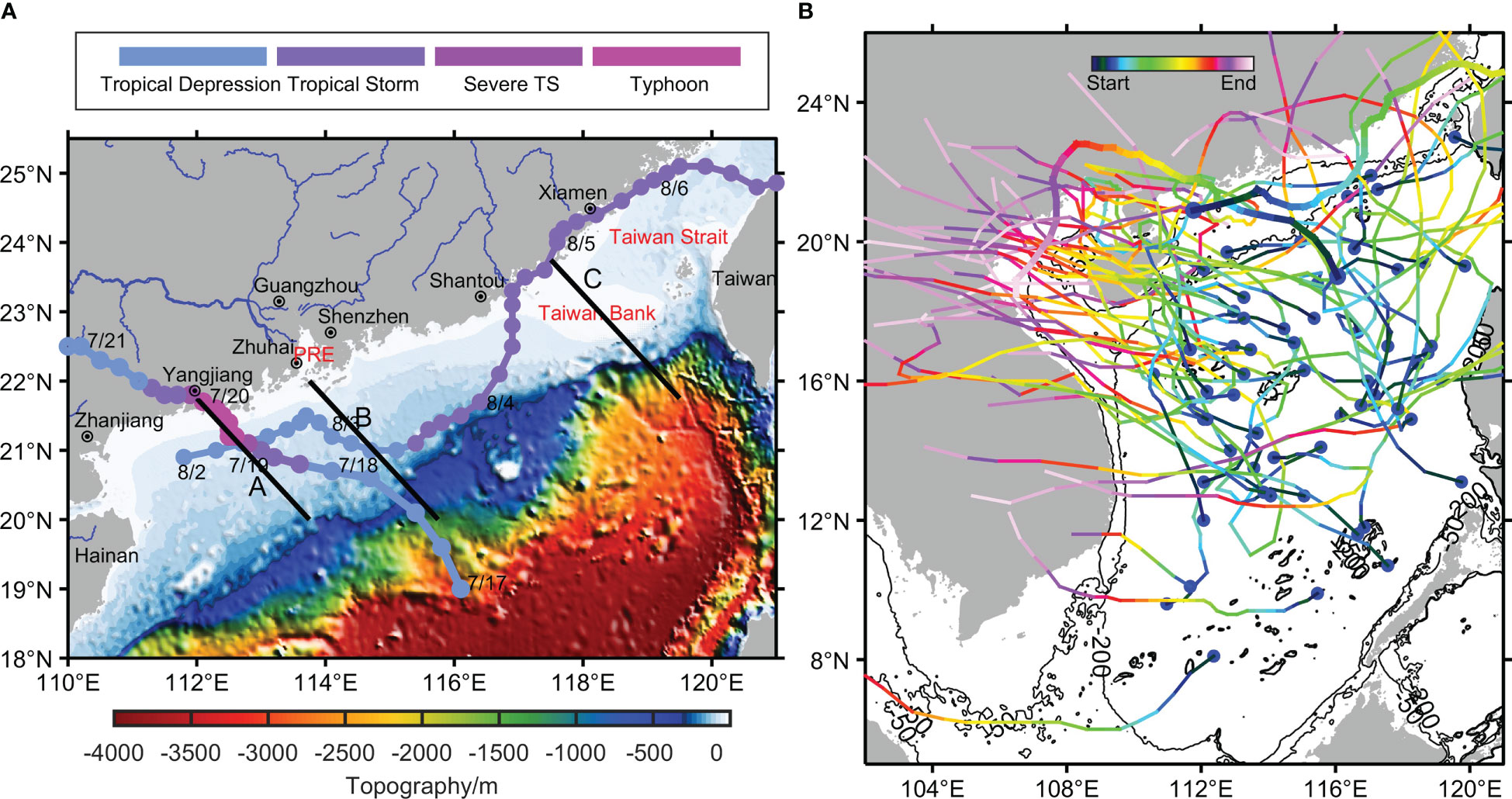
Figure 1 Intensity and path of Typhoons Cempaka and Lupit in the Northern SCS (A) and the trajectories of typhoons generated in the SCS during 2000–2021 (B). The black lines in (A) labeled A, B, and C are three sections across the continental shelf used to study the response of vertical structure in Section 3.5, and the blue lines are river courses. The Pearl River Estuary is marked as PRE.

Typhoons (also referred to as tropical cyclones) are one of the most destructive natural disasters on Earth. They are classified using the Saffir–Simpson intensity scale (Saffir, 1973; Simpson, 1974), ranging from category 1 (64–82 knots or 33–42 m s⁻¹) to category 5 (>137 knots or 70 m s⁻¹). Typhoons frequently occur in the Northwest Pacific and SCS (Chen et al., 2015). An annual average of 10.3 typhoons are active in the SCS (Wang et al., 2007), and they occasionally impact the northern SCS continental shelf (Figure 1B), causing profound physical and ecological changes in the upper ocean (Lin et al., 2003a; Lin et al., 2003b; Wu and Li, 2018; Qiu et al., 2019). Due to strong vertical mixing or upwelling induced by typhoons, subsurface cold water is transported upward to lower the sea surface temperature (SST). SST cooling ranges from 1 to 9°C in the open ocean, varying with typhoons’ intensity and translational speed (Lin et al., 2003a; Black and Dickey, 2008; Zhu et al., 2016; Yue et al., 2018). This cooling usually produces a cold wake along the track, on the right side in the Northern Hemisphere or the left side in the Southern Hemisphere (Leipper, 1967; Mrvaljevic et al., 2013). However, the SST response to a typhoon in coastal waters and on the continental shelf differs from that in the open sea because of local environmental conditions, such as complex topography and shoreline blocking (Lai et al., 2013). For example, typhoon-induced maximum SST drop can occur on the left of the typhoon path (Bingham, 2007; Liang and Ge, 2014), and the SST even increases after a typhoon passes the continental shelf (Xie et al., 2017). The SST recovers slowly via the subsequent air–sea heat exchange and oceanic processes, within a few days to a few weeks after a typhoon passes (Price et al., 2008; Wu and Li, 2018).

Typhoons can also stimulate phytoplankton bloom, which is the most significant biological characteristic after a typhoon passes (Wu et al., 2007; Zhao et al., 2008; Feng et al., 2022). Phytoplankton bloom, as measured by chlorophyll a (Chla) enhancement, occurs when nutrients from the subsurface or bottom are entrained to the euphotic zone by strong vertical mixing and upwelling or extra nutrients from river discharge. Chla enhancement has been confirmed in many individual cases and varies with different typhoons. For example, Typhoon Kai-Tak in 2000 triggered a 30-fold increase (Lin et al., 2003b), and Typhoon Damrey in 2004 resulted in a Chla bloom of approximately 4 mg m⁻³ in the offshore areas (Zheng and Tang, 2007). In addition, Chla enhancement occurs not only at the surface but also in the subsurface just above the thermocline, as reported by Hung et al. (2010).

Based on decades of typhoon data, researches have pointed out the association of Chla enhancement with water depth, typhoon’s intensity, and translational speed (Chen et al., 2017; Wang, 2020; Li and Tang, 2022). By comparing the response to typhoons for areas with three different water depths, Chen et al. (2017) found an increase in depth-integrated Chla, mainly in the coastal waters and continental shelf. Wang (2020) demonstrated Chla responses to slow-translation-speed typhoons in the SCS, mostly near coastal waters. Furthermore, a recent study revealed that both weak and slow-moving as well as strong and fast-moving typhoons were characterized by maximum Chla bloom with an increase of 0.23 mg m⁻³ on the continental shelf, whereas strong and slow-moving typhoons induce a larger Chla enhancement with an increase of 0.14 mg m⁻³ in the open sea (Li and Tang, 2022).

The above studies demonstrate the differences in typhoon-induced SST and Chla variations on the continental shelf from those in the open sea. However, although numerous studies have been performed on the impact of strong typhoons on the marine environment in the past decades, only a few have focused on their response to weak, slow-moving typhoons on the continental shelf. The two typhoon events, Typhoon Cempaka and Typhoon Lupit, discussed in this article have several characteristics. First, they were generated or strengthened on the continental shelf. Typhoon Cempaka originated on July 17, 2021 over the northern SCS slope and developed into a category 1 typhoon after entering the western Guangdong shelf and landed in Yangjiang on July 20. Typhoon Lupit was formed on August 2, 2021 in the coastal waters near Zhanjiang, quite close to the coast. It then migrated along the northern SCS shelf, and landing in Shantou on August 5 (Figure 1). Their trajectories changed, and they landed quickly. For example, Lupit’s track was opposite to the conventional native typhoon moving northwestward (Figure 1B), making it difficult to be forecasted (Zeng et al., 2022). Second, the maximum wind speeds (mean translation speeds) of Cempaka and Lupit in the northern SCS were 38 m s⁻¹ and 23 m s⁻¹ (1.9 m s⁻¹ and 2.6 m s⁻¹), respectively, as recorded by the Chinese Meteorological Administration (CMA). This suggests that they were weak and slow-moving, as mentioned by Zhao et al. (2008). Third, Cempaka (Lupit) brought heavy rainfall with a lasting and wide influence on Guangdong and Guangxi (Guangdong, Hong Kong, and Fujian).

In past decades, intensive studies have investigated SST and Chla in response to typhoons using multi-platforms like satellite observations (Lin et al., 2003a; Lin et al., 2003b; Yang et al., 2010; Wang, 2020) and in situ observations (Zhao et al., 2009; Liu et al., 2013; Qiu et al., 2019), as well as Bio-Argo (Chacko, 2017; Roy Chowdhury et al., 2022). Nevertheless, extreme weather conditions make field observation data difficult to obtain during most typhoon periods. In addition, the available satellite observation data are scarce because of heavy rainfall and cloud coverage during the typhoon period (Chang et al., 2008). For example, 50% of Chla data were unavailable (Wang, 2020), and the timing of maximum SST cooling might be inaccurate (Sun and Oey, 2015). Such non-uniform sampling in time and space often causes errors when quantifying the variations in SST and Chla during the typhoon period.

Therefore, numerical modeling is increasingly important in typhoon prediction and disaster assessment because it can untangle three-dimensional physical and ecological variations during extreme weather conditions. For example, we can further understand the fine-scale of circulation movement and temperature beneath typhoons (Sui et al., 2022) and chlorophyll change (Subrahmanyam et al., 2002). Moreover, changes in vertical structures, such as the warming of the subsurface layer, that cannot be captured by satellites can also be discovered by numerical modeling (Zhang et al., 2018). However, some undeniable model biases always exist compared to observations. Thus, inter-comparison and evaluation of different models with observations are necessary to decrease model errors and improve the forecast accuracy of marine changes as typhoons pass. Accurate predictions can reduce or prevent disasters, and have significant social and economic impacts in ensuring the safety of people’s lives and property.

The rest of this study is organized as follows: the typhoon, in situ, satellite data used in this study, and the regional and global Operational oceanography Forecasting Systems (OFS) are introduced in Section 2. Section 3 presents the results of the comparison, evaluation, and discussion between regional and global OFSs and in situ observations. Finally, Section 4 summarizes the conclusions of this paper.

2 Data, model, and method

2.1 Typhoon data

Data from successive typhoons Cempaka and Lupit were downloaded from the CMA (tcdata.typhoon.org.cn) (Lu et al., 2021). The records comprised several location time series, including the longitudes and latitudes of the typhoons’ centers, their maximum sustained wind speeds 10 m above the mean sea level, their central atmospheric pressures, and their statuses every 6 h or 3 h.

2.2 In situ data

Two summer cruises funded by the Southern Marine Science and Engineering Guangdong Laboratory (Zhuhai) were conducted in and near the PRE from July 27 to August 9, 2021, and August 2–8, 2022. There were 40 stations measured in 2021, among those labeled as red-filled circles in Figure 2 over the inner and western PRE observed before Typhoon Lupit (before August 3), while those labeled as purple-filled circles over the outside and eastern PRE sampled after Typhoon Lupit (August 6–8). The 28 sampling stations in 2022 coincided with some of those in 2021, but no observations occurred in bays on two sides of the PRE. Profiles of temperature, salinity, and depth were measured by a Conductivity–Temperature–Depth sensor (SBE 911 plus, SeaBird Scientific Inc.). Chla and turbidity were observed by a fluorimeter and a turbidity sensor at each station, respectively. Inorganic nutrient concentrations (nitrate) at the surface and bottom layers were analyzed by an Automated Flow Injection Analyzer 2000. The temperature and Chla at stations A1, A4, B3, B6, C2, and C5 were employed to verify the profile structures from the forecasting systems because those stations are quite close to the 1/4° grid point of biogeochemical products of MO. In addition, profiles before (A1, B3, and A4) and after (B6, C2, and C5) Lupit were used to compare and evaluate the forecasting systems with in situ observations during the pre- and post-typhoon periods.

FIGURE 2

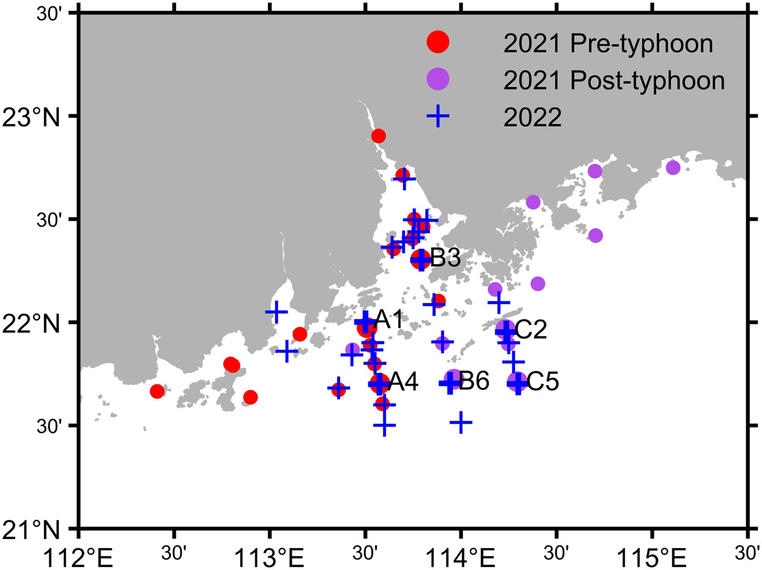
Figure 2 Location of sampling stations in and around the PRE in 2021 and 2022. The red- and purple-filled circles are the stations in before and after typhoon periods in 2021, respectively, and the blue “+” represents the stations in 2022. Stations A1, A4, B3, B6, C2, and C5 are used in this article.

2.3 Operational Forecasting Systems

2.3.1 Global Mercator Ocean Operational Forecasting System

The high-resolution global analysis and forecasting system GLO12v3 (previously called PSY4V3R1) was developed and maintained by Mercator Ocean (MO) in France and has operated as the MyOcean project since October 2016. The upgraded version, known as GLO12v4, has been available since November 2022 from Copernicus Marine Environment Monitoring Service, which produced weekly 14-day hindcasts and daily 10-day forecasts. The configuration is based on the tripolar ORCA12 grid type in version 3.6 of the NEMO ocean model (Madec et al., 2017) with a 1/12° horizontal resolution, corresponding to 9 km at the equator, 7 km at mid-latitudes, and 2 km toward the Ross and Weddell seas. The vertical resolution is 1 m at the surface, decreasing to 450 m at the bottom, with a total of 50 layers and 22 layers within the upper 100 m.

The sea surface atmospheric forcing comes from the European Centre for Medium-Range Weather Forecasts (ECMWF) Integrated Forecast System (IFS) at a 1/10° and 3 h resolution. Using a reduced-order Kalman filter method derived from a SEEK filter (Brasseur and Verron, 2006), multivariate data assimilation of oceanic observations, including in situ temperature and salinity (T/S) from Coriolis/Ifremer, along-track MSLA from AVISO, and intermediate resolution (0.25°×0.25°) SST product from NOAA, is performed with the SAM2 software (Lellouche et al., 2013; Lellouche et al., 2018). The biogeochemical module of MO is based on PISCES 3.6 as a part of the NEMO modeling platform (Aumont et al., 2015). The model is forced offline by the daily physical forecasts from MO and assimilates sea surface Chla data observed by the CMEMS-OCTAC satellite through the SAM2 Mercator Assimilation System filter. The horizontal resolution has a regular grid at 1/4°, with 50 vertical layers on the global ocean.

2.3.2 Regional SCS Operational Forecasting System

This study's regional high-resolution simulated results are from the SCS numerical ocean model, modified from the South China Sea Operational Oceanography Forecasting System (SCSOFSv2, Zhu et al., 2022). SCSOFSv2 is built on the Regional Ocean Modeling System (ROMS). The model’s boundaries were extended southward and eastward to cover a larger domain (4.5°S–28.3°N, 99°145°E) than the SCS. The horizontal resolution varies from 1/12° in the south and east boundaries to 1/30° in the SCS, with 50 layers in the vertical direction. When compared with SCSOFSv2, the open boundary conditions were changed from Simple Ocean Data Assimilation (SODA, Carton et al., 2018) version 3.3.1 and 3.3.2 monthly averages to SODA3.4.2 with a 5-day average during 1990–2020 and PSY4V3R1 with a daily average during 2021–2022. The surface atmospheric forcing replaces the 6-h Climate Forecast System Reanalysis (CFSR, Saha et al., 2010) for 1990–2011 and the Climate Forecast System version 2 (CFSv2, Saha et al., 2014) for 2011–2018 with the fifth-generation ECMWF Reanalysis (ERA5, Hersbach et al., 2020).

The other model configurations are the same as SCSOFSv2, except that the “Multi-source Ocean data Online Assimilation System” (MOOAS, Zhu et al., 2022) is excluded. This study uses the Carbon, Silicate, and Nitrogen Ecosystem (CoSiNE) model for biogeochemical stimulation, which is coupled online with ROMS. Fifteen state variables are considered: four nutrients (ammonium, nitrate, silicate, and phosphate), two phytoplankton groups (picophytoplankton and diatoms), two zooplankton groups (microzooplankton and mesozooplankton), two types of Chla, two types of detritus for simulating sinking and suspending, dissolved oxygen, total alkalinity, and total carbon dioxide. More detailed information can be found in Chai et al. (2002), Xiu and Chai (2014), and Zhang et al. (2023).

2.4 Satellite and reanalysis data

The Group for High-Resolution SST (GHRSST, Donlon et al., 2007) is a merged high temporal and spatial resolution SST product. Operational SST product at a 1 km spatial resolution is available from GHRSST. The input SST data consist of infrared (IR) sensors (e.g., AVHRR, METOP, MODIS, and AATSR), Geostationary Satellites (GOES, MTSAT, and SEVIRI/MSG), and microwave sensors (e.g., AMSR-E and TMI) with spatial resolutions of 1, 5, and 25 km, respectively. The field SST observations from ships, moorings, surface drifters, and profiling floats are also used. All the SST products are delivered with additional fields such as quality flags, standard deviation, and bias. More details about GHRSST products are available at http://www.ghrsst.org.

The daily and monthly satellite-derived sea surface Chla during Typhoons Cempaka and Lupit are provided by version 4.2 of the Ocean Colour Climate Change Initiative (OC-CCI), available online at https://esa-oceancolor-cci.org. The spatial resolution of OC-CCI is 4 km (Sathyendranath et al., 2019). OC-CCI Chla measurements integrate four distinct ocean color sensors: NASA-SeaWiFS, NASA-MODIS-Aqua, NASA-MERIS, and ESA-MERIS. Data are processed to be merged from these different platforms using the POLYMER v4.1 algorithm (MERIS) and SeaDAS v7.5 12gen tool (SeaWiFS, MODIS, and VIIRS) atmospheric-correction models. The OC-CCI Chla is well-validated with in situ observations in the global ocean (Valente et al., 2019) and used in the regional study (Guo et al., 2017).

2.5 SST anomalies and Chla changes induced by typhoons

The range of typhoon-induced SST cooling and phytoplankton blooms varies with typhoons' intensity and translational speed. For example, phytoplankton blooms were distributed in a region measuring 200 km across and 600 km along the typhoon trajectory in the Northwest tropical Pacific (Shibano et al., 2011). Typhoon-induced surface changes in Chla were observed within 300 km from its center, with major changes generally found within 100 km of the trajectory (Yang et al., 2010). Compared with previous research, Typhoons Cempaka and Lupit were relatively weak and moved only in the northern SCS shelf. Hence, this study focuses on the changes within 100 km of the typhoon center.

Oceanic responses to the typhoons were evaluated with SST anomalies (SSTA), obtained by removing the 2007–2021 average from the corresponding day at each pixel using Equation (1), referring to the study of Wang (2020):

$\begin{array}{ll}SST{A}_n\left(p,t\right)=SS{T}_n\left(p,t\right)-SS{T}_n{\left(p,t^{\prime }\right)}_{clim}& (1)\end{array}$

where, SSTA_n(p, t) are typhoon-induced SSTA at location n with respect to pixel p and time t. The pixel was less than 100 km from a typhoon center, and the date period was from 15 days before to 15 days after (-15–15 day) the typhoon’s arrival, SST_n(p, t) are the original time series, and SST_n(p, t’) _clim are the corresponding climatological averages for day t′ of a year at pixel p.

SSTA and Chla were spatially averaged at a daily interval to obtain a time series of typhoon-induced SSTA changes (SSTA_n(t)) and Chla changes (Chla_n(t)) at each typhoon location n and time t using Equations (2) and (3):

$\begin{array}{ll}SST{A}_n\left(t\right)=\frac{1}{N}{\sum }_{i=1}^{p}SST{A}_n\left(p,t\right)& (2)\end{array}$

$\begin{array}{ll}Chl{a}_n\left(t\right)=\frac{1}{N}{\sum }_{i=1}^{p}Chl{a}_n\left(p,t\right)& (3)\end{array}$

Finally, all Cempaka's and Lupit's locations with 3- or 6-h intervals are averaged to obtain the variations in SSTA and Chla from 15 days before to 15 days after the typhoon's arrival.

3 Results and discussion

3.1 Model validation

First, we verified the physical and biogeochemical results of SCSOFSv2 and MO. Zhu et al. (2016) comprehensively compared and verified the SCSOFS version 1 and MO results. They found that SCSOFS (MO) performed better in simulating the temperature and salinity structures (ocean circulations and the SST), and the SCSOFS simulation was better than MO in SST fronts and SST cooling during Typhoon Tembin compared with previous studies and satellite data. The domain-averaged monthly mean root-mean-square errors (RMSE) in SST and sea level anomaly simulated by SCSOFSv2 decreased from 1.21°C to 0.52°C and from 21.6 cm to 8.5 cm (Zhu et al., 2022), differing from the previous version. In general, both SCSOFSv2 and MO can provide science-based forecast of physical products that have been well-verified, so the validation of physical results is not repeated here. The reader is referred to two previous articles (Zhu et al., 2016; Zhu et al., 2022) for more verification details.

Both SCSOFSv2 and MO can correctly reproduce the sea surface Chla distribution pattern compared with satellite observations in July and August 2021 (Figure 3). High Chla (>0.5 mg m⁻³) is spread in the PRE, coastal waters, Taiwan Strait, and Taiwan Bank, whereas Chla is below 0.2 mg m⁻³ on the continental shelf and open sea (Figures 3A–F). Satellite observations and simulated Chla show a large difference, ranging from 0.2 to 2 mg m⁻³ on coastal waters and the continental shelf (Figures 3G–J). SCSOFSv2 Chla is lower than the observations in the coastal waters, the eastern Leizhou Peninsula and the eastern Guangdong shelf in July, but higher than the observations in the PRE-western Guangdong shelf in July and the PRE-eastern Guangdong shelf in August (Figures 3G, H). MO Chla is lower than the observations in coastal waters and the eastern Guangdong shelf in August and higher than the offshore observations of the PRE, Taiwan Bank, and Taiwan Strait (Figures 3I, J). These differences can be attributed to several reasons, such as the accuracy of reproducing mixing and upwelling events, runoff discharge, tide and wave processes, suspended and resuspended sediments, and the high uncertainties of satellite chlorophyll observations in coastal regions. In the open sea, SCSOFSv2 (MO) Chla is lower (higher) than the observations in both July and August (Figures 3G–J).

FIGURE 3

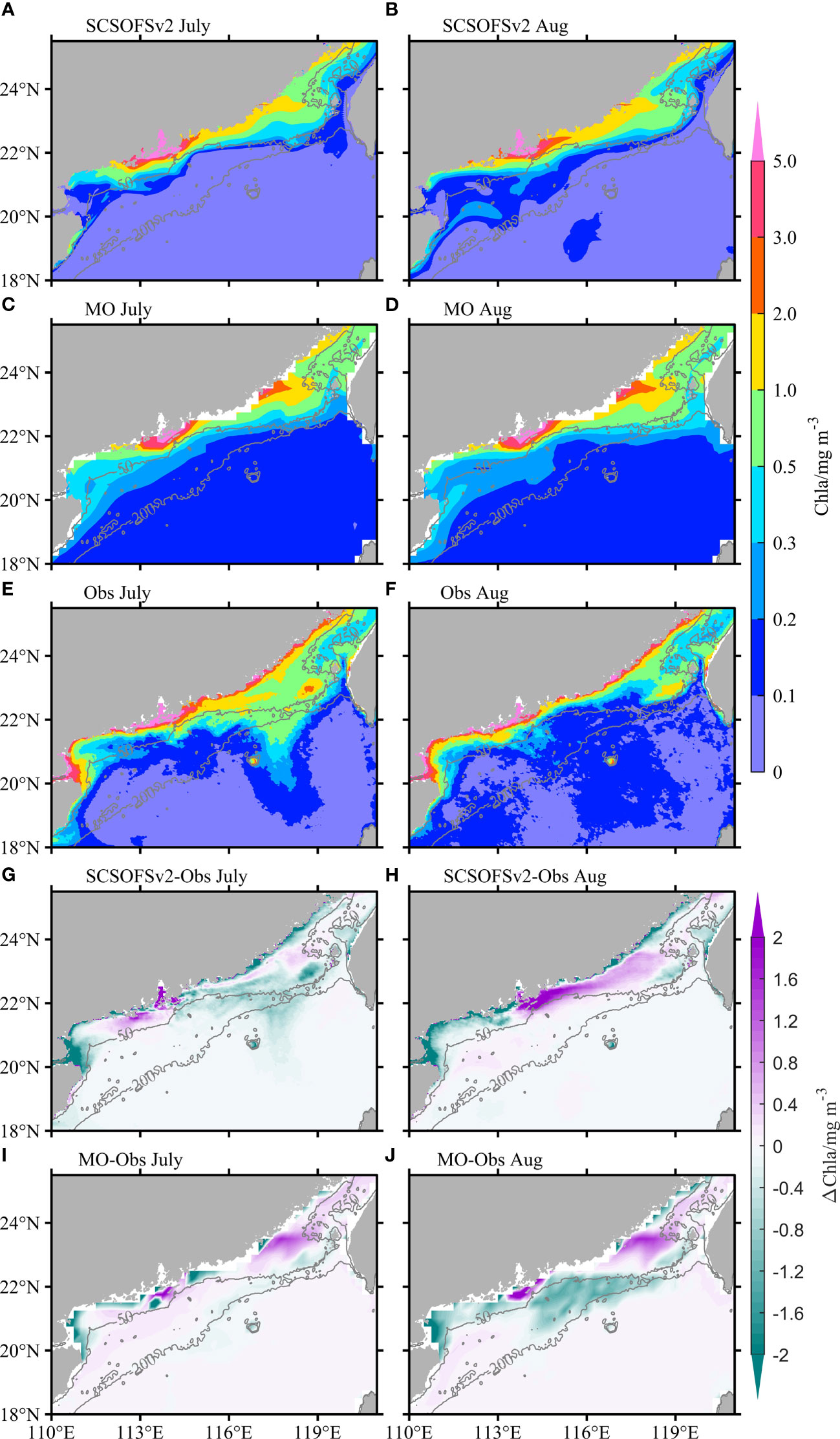
Figure 3 SCSOFSv2, MO, and observed sea surface Chla (A–F) and corresponding differences (G–J) in July (left) and August (right) of 2021. Observed monthly mean Chla is provided by OC-CCI version 4.2. The gray lines are 50 m and 200 m isobaths.

The validation is further assessed on the shelf region and open sea. The validation results with correlation coefficients and RMSEs are shown in Figure S1. This figure shows well-simulated results on the shelf with a high correlation coefficient between 0.59 and 0.72 at a 99% confidence level (CL) between simulated and observed Chla. The high background values (0.1 to over 15 mg m⁻³) there induce a large Chla RMSEs from 0.61 to 0.69 mg m⁻³ (Figures S1A, B). By contrast, correlation coefficients between the model and observations range from 0.21 to 0.45 at 95% CL in the open sea, and the small background values (generally below 0.1 mg m⁻³) result in low RMSEs ranging from 0.03 to 0.078 mg m⁻³ (Figures S1C, D). In general, Chla simulated by SCSOFSv2 and MO can reproduce the Chla distribution, and each has its respective merits.

3.2 In situ observations in the PRE

The PRE is a major estuary situated at the Guangdong coastal waters with China's second-largest freshwater discharge (Zhao, 1990). Typhoons Cempaka and Lupit were closed to the PRE, inducing profound oceanic variations, such as the SST and near-inertial oscillations in the coastal waters at Jitimen (Chen et al., 2022). Here, the 2021 in situ temperature, Chla, and NO₃ profiles are used to evaluate and compare the SCSOFSv2 and MO simulations during Lupit. In addition, the profiles sampled in the same period in 2022, without active typhoons, are used to highlight the variations induced by Lupit.

The observed temperature profile exhibits a little difference at A1 between 2021 and 2022, and it is lower in 2022 than in 2021 at B3, whereas it is 2–4°C lower in 2021 than that in 2022 at A4, B6, C2, and C5 (Figure 4, upper panel). In addition, the vertical gradient in temperature and the thermocline in 2021 at B6, C2, and C5 as Lupit passed is significantly weaker than that during the pre-typhoon period in 2021 at B3 and in 2022 at B6, C2, and C5. This difference reveals the profound effect of typhoon-induced mixing on the vertical temperature structure at these stations. SCSOFSv2 and MO temperatures are consistent with the observed temperatures (Figure 4, upper panel, and Figure S2A). The upper layer simulation agrees well with the observation with an approximate error of 0.5°C at the surface, and the error of SCSOFSv2 is greater than that of MO below 10 m. The maximum error depth of MO is at 6 m, whereas SCSOFSv2 appears at 33 m (Figure S3A). The correlation coefficients between the SCSOFSv2 and MO profiles and in situ observations are 0.93 and 0.95 at 99% CL, and the RMSEs are 1.24 °C and 0.84 °C, respectively (Figure S2A and Table 1). This suggests a comparatively better MO simulation of the temperature structures than SCSOFSv2 in the PRE.

FIGURE 4

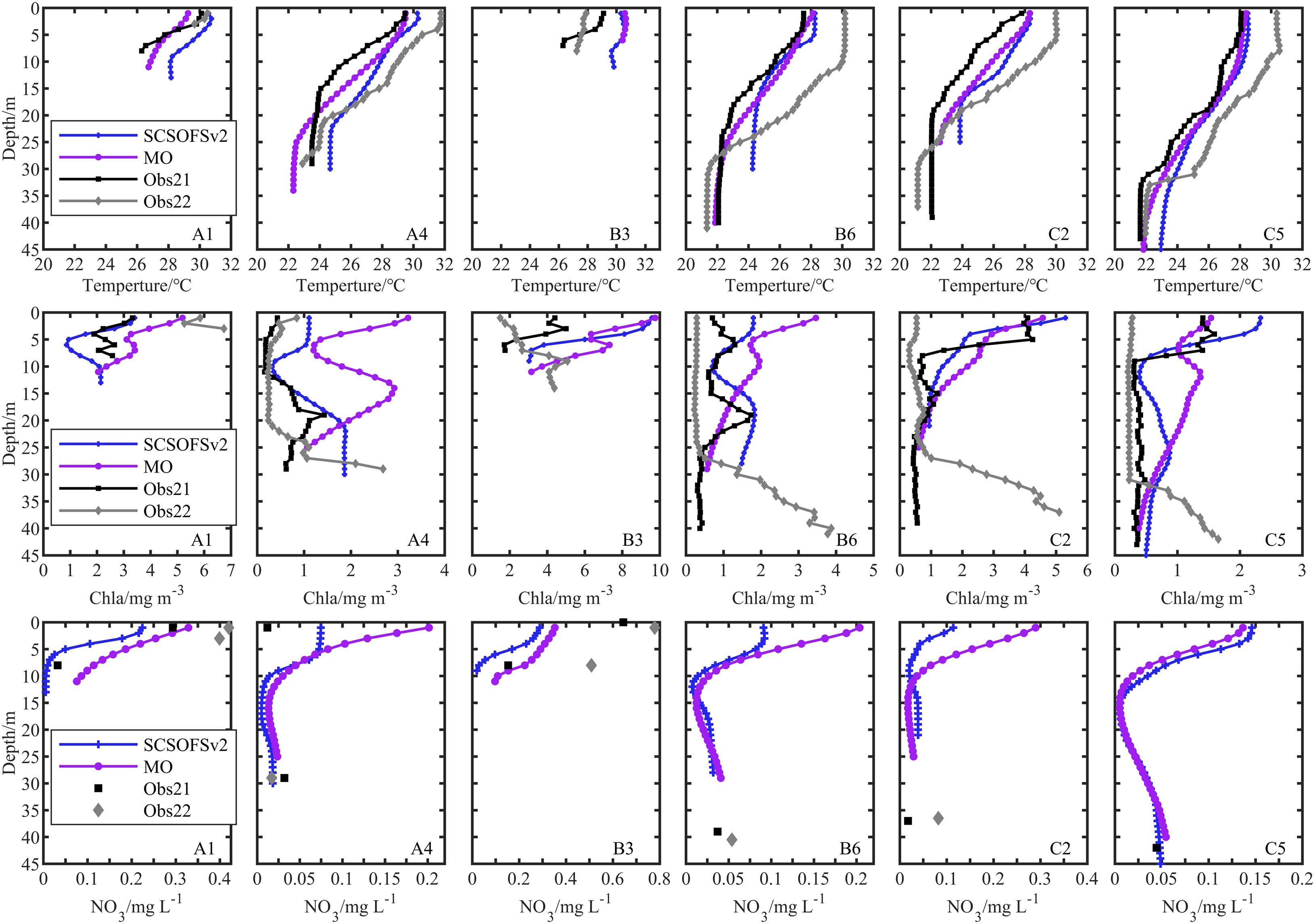
Figure 4 Temperature (upper panel), Chla (middle panel), and NO₃ (bottom panel) profiles at A1, A4, B3, B6, C2, and C5. Profiles simulated by SCSOFSv2 and MO are interpolated to 1-m intervals to coincide with the observations. It is noted that the tick labels of the x-axis in the middle and bottom panels vary with the different stations.

TABLE 1

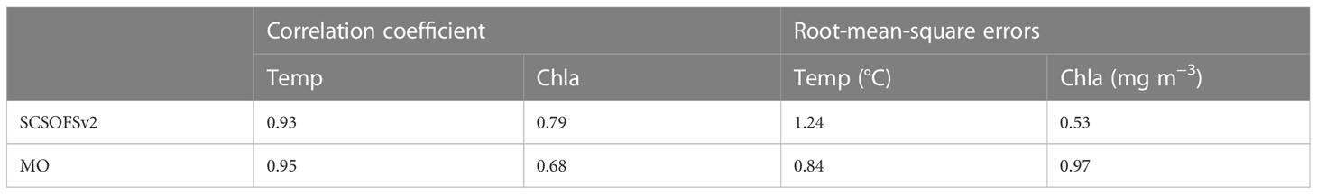
Table 1 Correlation coefficient and root-mean-square errors between simulated and observed temperature and Chla at A1, A4, B3, B6, C2, and C5.

Observed Chla is much higher in 2022 than in 2021 at A1, whereas the upper Chla at A4 in 2022 is the same as that in 2021, but the bottom Chla is higher than the surface layer in both 2021 and 2022. Similarly, observed low and high Chla dominate the upper and bottom layers at B3, B6, C2, and C5 in 2022, respectively (Figure 4, middle panel). A previous study found that surface nutrient loadings, along with runoff discharge, rapidly decreased seaward. This was because of both phytoplankton uptake and diffusion by seawater, which had a limited impact on phytoplankton growth in the offshore waters at A4, B6, C2, and C5 compared with that in the coastal and estuarine areas at A1 and B3 (Song et al., 2011). In addition, the depth of the Chla maximum (DCM) did not appear in the subsurface layer, possibly due to the low turbidity (Figure S4) of seawater in 2022. This suggests that more light transmission into the bottom layer benefits phytoplankton photosynthesis, leading to a significant Chla increase at the bottom layer. By contrast, the Chla profiles at B6, C2, and C5, observed after Lupit’s arrival in 2021, featured high values on the surface but low values at the bottom layer, displaying an apparent discrepancy with the 2022 observations. This is because Lupit-induced strong mixing or upwelling uplifted bottom nutrients to the surface, resulting in Chla enhancement at the surface (Wu et al., 2007; Zhao et al., 2009; Feng et al., 2022).

The SCSOFSv2 and MO simulations are overall similar to the structures observed in 2021. SCSOFSv2 Chla is much closer to the observations at the upper layer of A1, A4, and B6. The upper simulation at A1 is especially consistent with the observations, whereas the upper Chla simulated by MO agrees more with the observations at C2 and C5. In the near-bottom layer, the SCSOFSv2 and MO simulations coincide with the observations, except for A4 and B6, where SCSOFSv2 is larger than the observations (Figure 4, middle panel). Generally, the surface layer exhibits the largest Chla error, approximately 1.5 mg m^-3, whereas the SCSOFSv2 error is lower overall than for MO below the subsurface layer (Figure S3B). The correlation coefficient between SCSOFSv2 and observations at the six stations is 0.79 at 99% CL, and the RMSE is 0.53 mg m⁻³, which is better than the MO simulation having a correlation coefficient of 0.68 at 99% CL and the RMSE at about 0.97 mg m⁻³ (Figure S2B and Table 1).

NO₃ profile variations are shown in the bottom panel of Figure 4. Surface NO₃ at coastal stations A1 and B3 is larger than that at the bottom in both 2021 and 2022, opposite to offshore station A4 in 2021. Bottom NO₃ at A4 in 2021 is higher than in 2022, whereas bottom NO₃ at B6 and C2 in 2021 is lower than in 2022, proving that the decrease of bottom NO₃ is because of Lupit-induced upward transport. The bottom NO₃ simulations of both profiles are very close to the observations. However, the surface NO₃ simulations reveal a clear difference from the observations. Surface NO₃ from SCSOFSv2 and MO are lower by approximately 0.07 mg L⁻¹ and higher by 0.04 mg L⁻¹ than the observation at A1, respectively, and are 0.06 mg L⁻¹ and 0.19 mg L⁻¹ higher than the observation at A4, respectively (Figure 4, bottom panel).

3.3 Response of SST

SST cooling is one of the predominant characteristics after a typhoon’s arrival (Lin et al., 2003a; Black and Dickey, 2008; Mrvaljevic et al., 2013; Yue et al., 2018). Figure 5 shows the SST difference compared to the previous days of July 20, July 24, August 4, and August 9, during the Cempaka and Lupit periods. A clear SST cooling center is observed in the SCSOFSv2 and MO simulations, but it is not apparent in GHRSST when Cempaka landed in Yangjiang on July 20 (Figures 5A–C). Unlike the SST drop in most sea areas, both the simulated and observed SSTs in the western Guangdong shelf increased by 0.5–1.0°C (Figures 5D–F) on July 24, which provided energy for the subsequent Typhoon Lupit. Lupit migrated to the northeastward along the continental shelf and landed in Shantou on August 5. The SST decreased significantly in the northern SCS on August 4 compared to the previous day. The SCSOFSv2 SST decrease in the Shantou nearshore was larger than that for MO and GHRSST, whereas SST changes were more consistent with MO and GHRSST in the other regions (Figures 5G–I). After Lupit’s arrival, SST recovered on August 9. SCSOFSv2 and MO SST increased in most areas of the northern SCS, and the MO SST rise was especially pronounced, exceeding 1.5°C around the Hainan Inlands. However, GHRSST increases only occurred in the central part of the northern SCS, but continued to fall in the surrounding regions (Figures 5J–L).

FIGURE 5

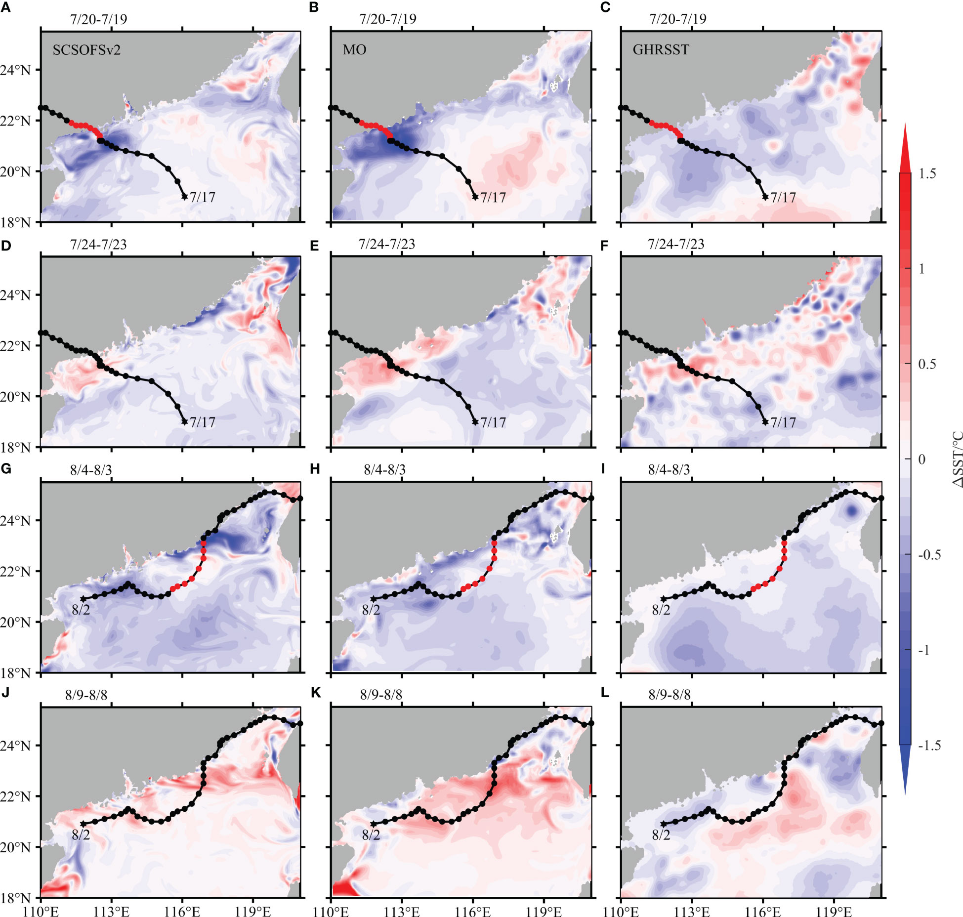
Figure 5 Variations of the SST difference (∆SST) compared to the previous days of July 20 (A–C), July 24 (D–F), August 4 (G–I), and August 9 (J–L) during the typhoon period. The first, second, and third columns are the maps from SCSOFSv2, MO, and GHRSST, respectively. The black line represents the typhoon path, with red dots labeled as the typhoon’s centers on the present day, and the asterisk indicates the place of typhoon genesis at the start time.

The variations of SSTA 15 days before and after (-15–15 day) the typhoon’s arrival are calculated to analyze the SST response to Cempaka and Lupit quantitatively. Cempaka- and Lupit-induced SSTA changes are vastly different (Figure 6). SSTA increased from -12 day to -5 day, and peaked at about 1.2°C at five days before Cempaka’s arrival. As Cempaka approached, the SSTA dramatically decreased with a smaller positive anomaly. The GHRSST anomaly decreased to a minimum of approximately 0.52°C two days after the passage of Cempaka, but both SCSOFSv2 and MO SSTA dropped to approximate minima of 0.27°C and 0°C, respectively, one day after the passage of Cempaka, followed by simulated and observed SSTA recovery to 0.6–0.8°C within 8–9 days (Figure 6A). Before Lupit’s arrival, SSTA was between 0.3 and 0.6°C, with no notable SST rise. SCSOFSv2 and MO SSTA declined from -7 day to -6 day, whereas GHRSST declined starting five days before Lupit’s arrival. The SSTA shifted from positive to negative after the passage of Lupit. The minimum GHRSST anomaly was about −0.43°C, four days after Lupit’s arrival, consistent with previous studies that reported the SST reached a minimum four days after a typhoon’s arrival (Chang et al., 2008). SCSOFSv2 and MO SSTA fell to minimum values about −0.75°C and −0.92°C, respectively, two days and one day after Lupit’s arrival. Both simulated and observed SSTA recovered to the climatological condition 15 days after Lupit’s arrival (Figure 6B). These observations indicate the release of redundant heat on the continental shelf through these two consecutive typhoon events, to regulate the warmer SSTA to a normal condition.

FIGURE 6

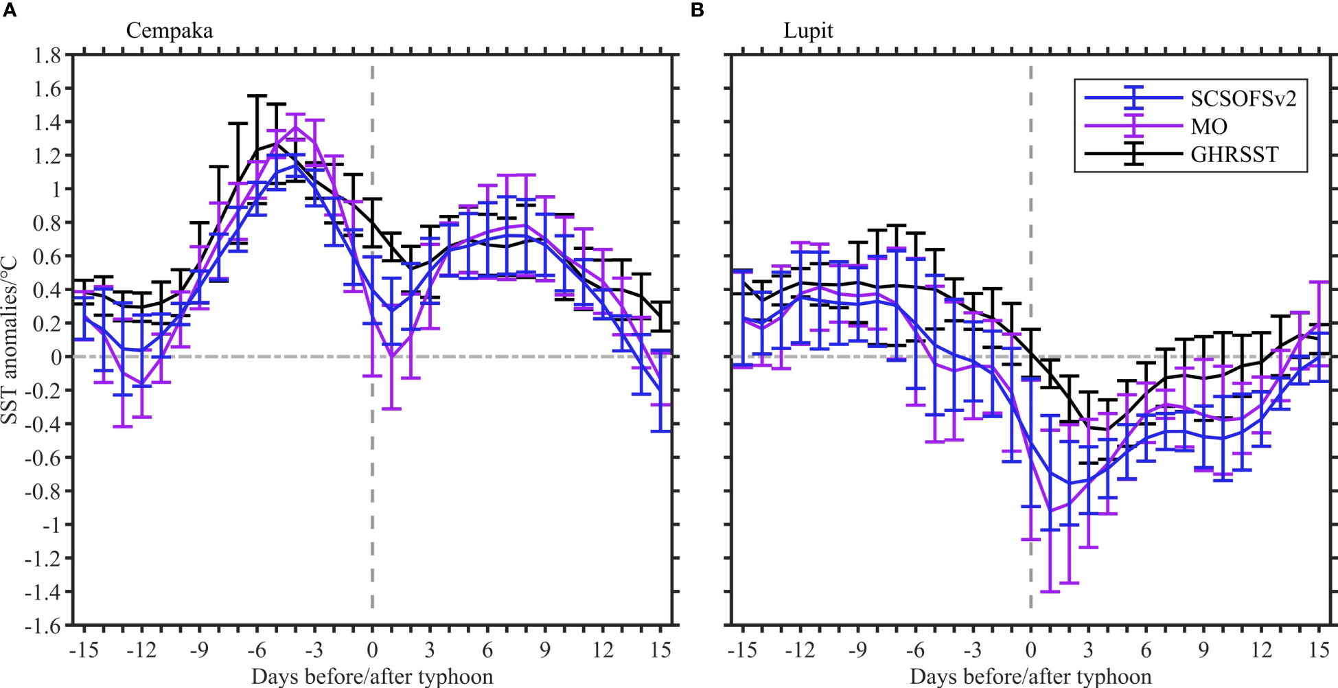
Figure 6 Daily variations of SSTA from 15 days before to 15 days after Cempaka (A) and Lupit (B). The blue, purple and black lines indicate SCSOFSv2, MO and GHRSST, respectively.

The above simulations also exhibit that both SCSOFSv2 and MO SSTA accurately reveal the actual variations compared with the observations. However, there are still two differences between the models and the observations. On the one hand, the timing of the maximum SST drop is 1 day and 2–3 days ahead of the observations during the Cempaka and Lupit periods, respectively. On the other hand, the SST cooling amplitudes are larger than the observations. SCSOFSv2 SSTA is closer to the observation, but MO SSTA is lower than the observation. The correlation coefficients between SCSOFSv2 SSTA and GHRSST anomalies during Cempaka and Lupit are 0.85 and 0.86 at 99% CL, respectively, which are higher than for the MO results. Meanwhile, the SCSOFSv2 SSTA RMSEs are 0.28°C and 0.34°C for the two typhoons, respectively, which are lower than for the MO results (Table 2). Therefore, the SSTA variation of SCSOFSv2 is more consistent with the observation than that of MO, which agrees with a previous comparison (Zhu et al., 2016).

TABLE 2

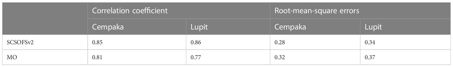
Table 2 Correlation coefficient and root-mean-square errors between simulated and observed SSTA from 15 days before to 15 days after Cempaka and Lupit.

3.4 Response of sea surface Chla

Sea surface Chla enhancement is another significant feature after a typhoon passes (Lin et al., 2003b; Chen et al., 2017; Wang, 2020). Both SCSOFSv2 and MO Chla reflect this variation well. Chla was below 0.2 mg m⁻³ on the western Guangdong shelf, and below 0.5 mg m⁻³ even in the coastal waters when Cempaka was generated on July 17 (Figures 7A–C). By contrast, after Cempaka’s arrival on July 23, high Chla levels extended from the PRE to the western of Zhanjiang coastal waters, increasing from 0.1–0.5 mg m⁻³ on July 17 to 0.2–5 mg m⁻³ on July 23 (Figures 7D, E). Satellite observation revealed a striking Chla enhancement July 23 on the western Guangdong shelf (Figure 7F), which verified the model’s Chla increase. Cyclonic wind during the Cempaka period (Figures S5A, B), when compared to before the typhoon passage, induced the extension of the river plume to the western Guangdong shelf (Figures S6C, D), which was consistent with the areas of Chla bloom. However, the observed Chla bloom along Cempaka’s track was larger than the model's because the ERA5 maximum wind speed driving SCSOFSv2 and MO is considerably smaller than the forecast from the CAM and the Cross-Calibrated Multi-Platform (CCMP) dataset (Figures S5A, B). Therefore, the ERA5 wind stirs a weaker nutrient mixing in SCSOFSv2 and MO during the Cempaka period, resulting in a relatively smaller Chla bloom than in the satellite observation.

FIGURE 7

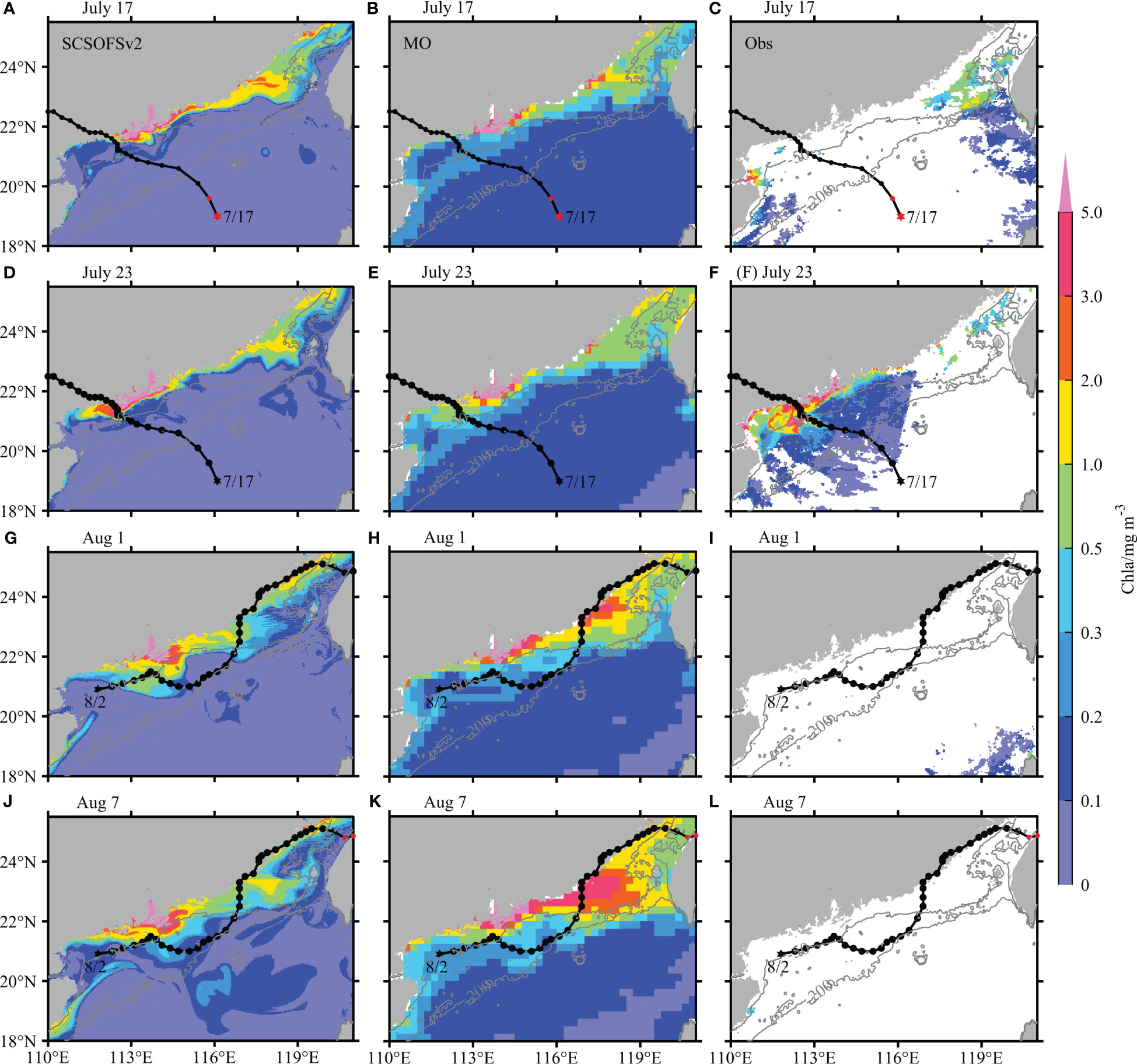
Figure 7 Variations of Chla before and after Cempaka and Lupit on July 17 (A–C), July 23 (D–F), August 1 (G–I), and August 7 (J–L). The first, second, and third columns are the maps from SCSOFSv2, MO, and observations provided by OC-CCI, respectively. The black line represents the typhoon path with red dots labeled as the typhoon’s centers on the present day, and the asterisk indicates the place of typhoon genesis at the start time. The gray lines are 50 m and 200 m isobaths.

Before the formation of Lupit on August 1 , high simulated Chla was distributed in and near the PRE, the eastern Guangdong coastal waters, and the Taiwan Strait (Figures 7G, H). High Chla extended seaward from coastal waters to the continental shelf after the passage of Lupit. Chla enhancement was most remarkable in the Taiwan Bank, increasing by 0.5–1.0 (0.5–2.5) mg m⁻³ from SCSOFSv2 (MO) compared with that on August 1 (Figures 7J, K). This indicates that Lupit was weak and slow-moving but still capable of causing Chla bloom along the continental shelf. As Lupit passed, the river plume extended to the outer PRE on August 4, which was quite different from the pattern on August 1 (Figures S6E–H) that resulted in Chla bloom. However, the southwest wind strengthened in the northern SCS during the Lupit period August 3–7, when compared to August 2, to produce a long-lasting vertical mixing and stronger upwelling along the continental shelf (Figure S7), uplifting more nutrients to stimulate a phytoplankton bloom and also Chla enhancement. Recent research has also found that slow-moving typhoons induce the most pronounced Chla increase on the continental shelf, consistent with that caused by strong and fast-moving typhoons (Li and Tang, 2022). Heavy rainfall and cloud coverage blocked the satellite observation of Chla during the Lupit period in the northern SCS (Figures 7I, L), so it cannot be used to verify the simulation results. Hence, it is necessary to predict and study the ecological response to typhoons by numerical modeling, because only a few observation data are available during the typhoon period (Chang et al., 2008).

To further evaluate typhoon-induced Chla bloom, Figure 8 shows changes in Chla averaged over a 100-km range at each typhoon’s center with the corresponding locations’ means from 15 days before to 15 days after Cempaka and Lupit. Cempaka migrated across the continental shelf from the slope and then landed in Yangjiang. Chla displays two change characteristics. First, a pronounced Chla enhancement occurs after Cempaka crosses the continental shelf (Figures 8A, B). The mean Chla increase predicted by SCSOFSv2 (MO) is about 0.64 (0.41) mg m⁻³, and SCSOFSv2 Chla bloom is higher than that for MO (Figure 8C). Second, the bloom timing of Chla is faster in coastal waters than on the continental shelf, in which SCSOFS (MO) Chla bloom occurred after four (three) and 2–3 (1–2) days on the continental shelf and coastal waters, respectively. Averaged Chla reached a maximum 3 (2) days after Cempaka passed. During the Lupit period, variations of SCSOFSv2 and MO Chla on the western Guangdong shelf and near the PRE were similar. Cempaka caused Chla bloom from 12 to 8 days before Lupit near the PRE (Figures 8D, E). However, variations in SCSOFSv2 Chla on the eastern Guangdong shelf and in the waters around Taiwan Island were too weak to reveal typhoon-induced Chla bloom (Figure 8D). MO Chla bloom occurred in the above region, especially in the eastern Guangdong coastal waters. MO Chla increased to a maximum (>3.0 mg m⁻³) two days after Lupit’s arrival, which was about two times the level before its arrival, and then dropped sharply (Figure 8E). MO mean Chla increased by 0.41 mg m⁻³, almost equal to the Chla increase induced by Cempaka (Figures 8C, F).

FIGURE 8

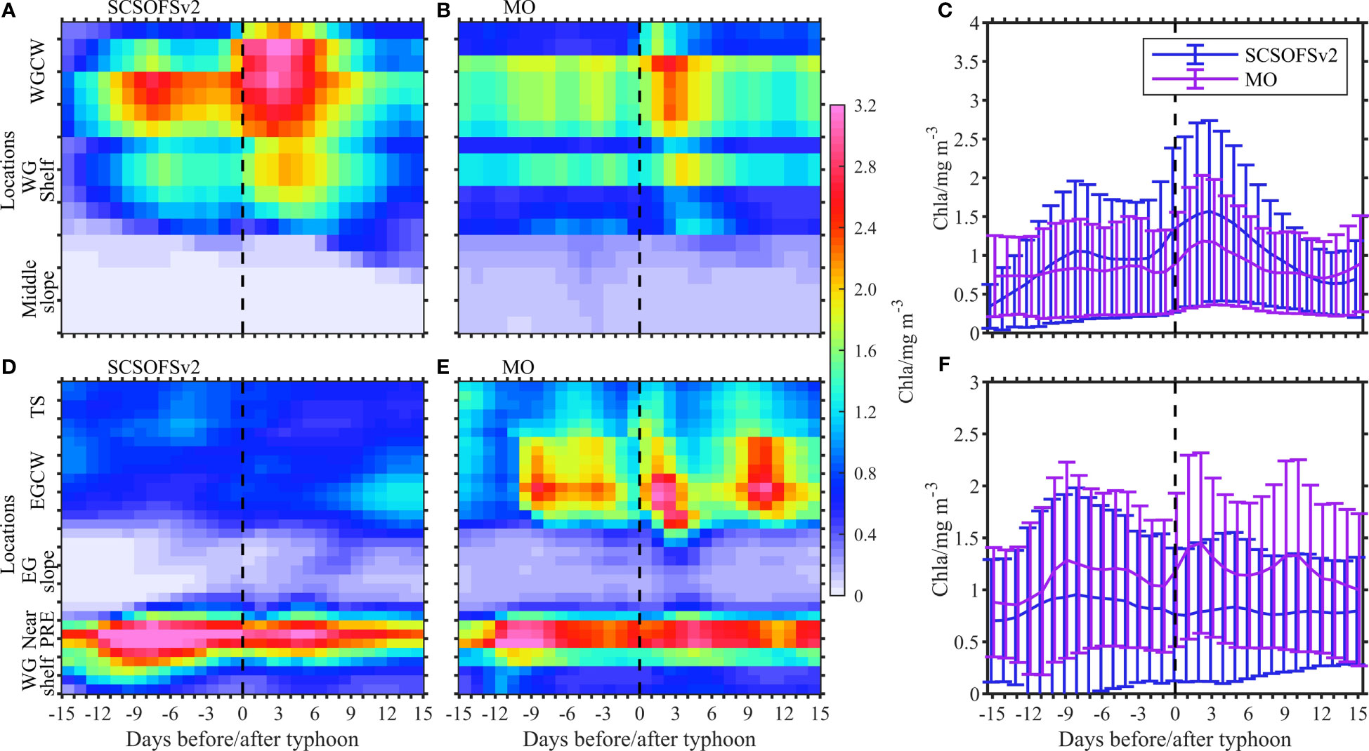
Figure 8 Variations of Chla averaged by a 100-km range of typhoons’ center from 15 days before to 15 days after Cempaka from SCSOFSv2 (A), MO (B) and Lupit from SCSOFSv2 (D), MO (E) with corresponding locations’ means during Cempaka (C) and Lupit (F) from SCSOFSv2 (blue line), MO (purple line). The geographic location is labeled in the y-axis, in which WG, EG, WGCW, and EGCW denote the western and eastern Guangdong, and the western and eastern Guangdong coastal waters, respectively. PRE and TS are the Pearl River Estuary and the Taiwan Strait, respectively.

In general, the Cempaka-induced maximum Chla represented by SCSOFSv2 and MO and the Lupit-induced maximum Chla represented by MO were observed 2–3 days after the typhoon passed. This was 2 days ahead of the average (4–5 days) on the SCS shelf (Li and Tang, 2022), and several days ahead of the timing in the open sea, such as 6 days induced by Typhoon Linfa (Chen and Tang, 2012) and 13 days induced by Typhoon Nangka (Qiu et al., 2019). In addition, Cempaka- and Lupit-induced Chla bloom was significantly stronger than the approximate mean increase of 0.18 mg m⁻³ on the SCS shelf and 0.07 mg m⁻³ in the open sea, respectively (Li and Tang, 2022). The following two aspects can explain these differences. First, typhoons can stir and mix summer stratification in more vulnerable shallower waters (Chen et al., 2017). Second, slow-moving typhoons may produce a long-lasting mixing and upwelling to transport more subsurface or bottom nutrients to the surface on the continental shelf, stimulating a faster and stronger Chla enhancement (Zhao et al., 2008). Conversely, the oceanic response to typhoons in the open sea is longer than that on the continental shelf, and nutrient transportation from the bottom to the surface induced by wind is limited (Chen et al., 2009). Hence, Chla bloom is relatively weak in the open sea as reported by Li and Tang (2022).

3.5 Response of vertical structure

This study emphasizes the oceanic and ecological responses to typhoons. Accordingly, we have selected three sections across the western Guangdong shelf, the PRE and its outer shelf, and the eastern Guangdong shelf, respectively, marked as Sections A, B, and C in Figure 1A. These sections are used to analyze the variations of temperature, Chla, and NO₃ structures during the typhoon period.

3.5.1 Temperature structure

Section A reflects the changes in temperature before and after Cemkapa’s arrival, in which temperature cooling occurred on the surface layer and subsurface layers (Figures 9A, C). The upper temperature at Section A was greater than 30°C, with a maximum exceeding 32°C on July 17, whereas it dropped to less than 30°C after the typhoon passed. Isotherms were uplifted toward the surface, indicating the upward movement of the cold bottom water. Upwelling of the cold bottom water was most significant in the middle western Guangdong shelf after Cempaka passed (Figure 9A). Section A crossed the center of Cempaka, and changes in temperature at Section B were weak in comparison, with a clear decrease in the surface temperature, although the upwelling of cold water was quite limited (Figure 9C). Both sections revealed the uplifting of isotherms toward the surface, with a striking decrease in the upper temperature (Figures 9B, D, E). These isotherms became more vertical in the Taiwan Bank after Lupit passed (Figure 9E), suggesting that Lupit-induced strong mixing broke the original upwelling process. Overall, changes in the two models are consistent with each other. A large difference is that the bottom temperature of SCSOFSv2 is higher on the shelf than that for MO similar to the high bottom temperature error in the PRE (Figure S3A).

FIGURE 9

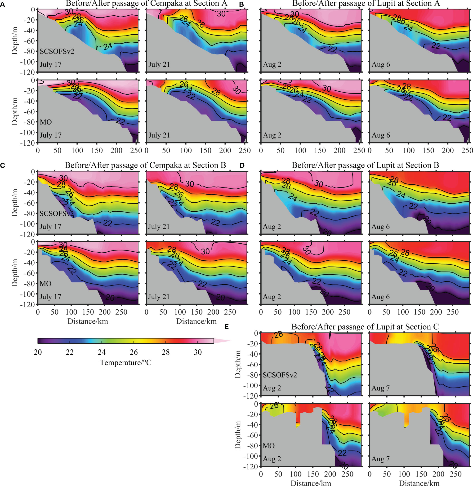
Figure 9 Temperature variations at Section A (A, B), Section B (C, D), and Section C (E) on the continental shelf during before and after Cempaka and Lupit. Data provided by SCSOFSv2 or MO is labeled on the first map of each row and the date has been marked on each map. The black lines represent isotherms with 2°C interval.

3.5.2 Chla structure

Chla changes are revealed in Sections A and B, before and after Cempaka’s arrival (Figures 10A, C). Compared with July 17, high surface Chla extended from the nearshore to the shelf about 100–150 km away from the coastline, and vertical Chla also increased on July 23 after Cempaka passed (Figure 10A). High Chla was observed at Section B in and near the PRE, and subsurface Chla also increased on July 25 on the continental shelf (Figure 10C). However, Cempaka’s impact was quite limited in Section C, where the typhoon center was hundreds of kilometers away, so the change in this region is not analyzed here.

FIGURE 10

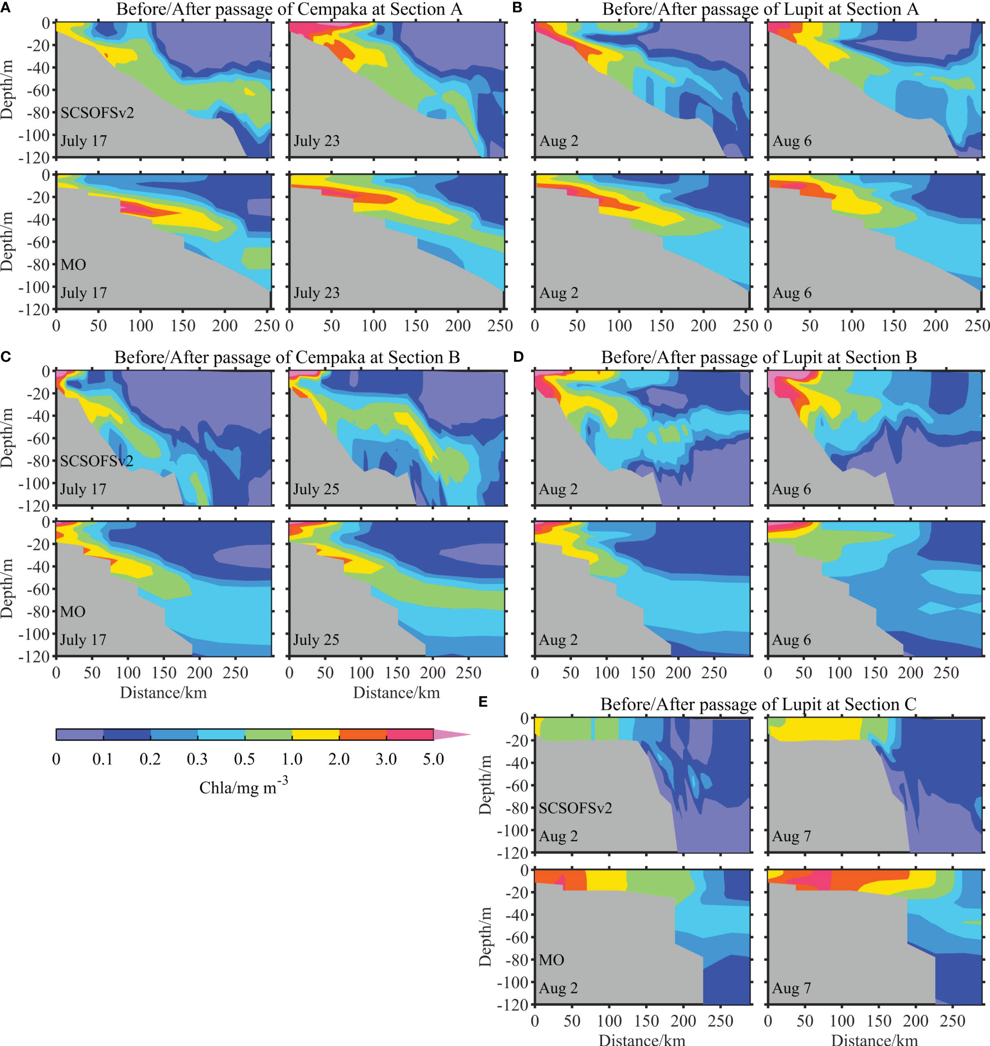
Figure 10 Chla variations at Section A (A, B), Section B (C, D), and Section C (E) on the continental shelf during before and after Cempaka and Lupit. Data provided by SCSOFSv2 or MO is labelled in the first map of each row and the date has been marked in each map.

During the Lupit period, the Chla change was striking in the three sections from west to east. Compared with August 2, nearshore surface Chla at Sections A and B peaked on August 6. Surface Chla simulated by SCSOFSv2 and MO extended seaward, and upper Chla increased from 0.1–0.2 mg m⁻³ to 0.2–0.5 mg m⁻³ on the continental shelf (Figures 10B, D). In Section C, both SCSOFS and MO Chla bloom occurred from coastal waters to the Taiwan Bank and even to the open sea on 7 August, 1–2 days after Lupit’s arrival (Figure 10E).

3.5.3 NO₃ structure

Chla enhancement is inseparable from the supply of nutrients such as nitrate (NO₃) and phosphate (Wu et al., 2007; Herbeck et al., 2011; Qiu et al., 2019). In this study, we chose NO₃ as the representative nutrient to analyze the vertical changes for which N was considered as the limiting nutrient for primary productivity in the northern SCS (Chen, 2005; Liu et al., 2010). Compared with July 17, NO₃ increased significantly in the nearshore at Section A on July 23 and Section B on July 25 after the passage of Cempaka. The SCSOFSv2 and MO NO₃ levels surpassed 0.1 mg L⁻¹ Sections A and B in the nearshore waters, respectively (Figures 11A, C). In addition, high NO₃ uplifted from the bottom to the subsurface to a certain extent. For example, SCSOFSv2 NO₃ was transported from the bottom to the middle layer, and the range of low NO₃ (<0.005 mg L⁻¹) simulated by MO at the middle and upper layers was compressed after Cempaka’s arrival (Figures 11A, C).

FIGURE 11

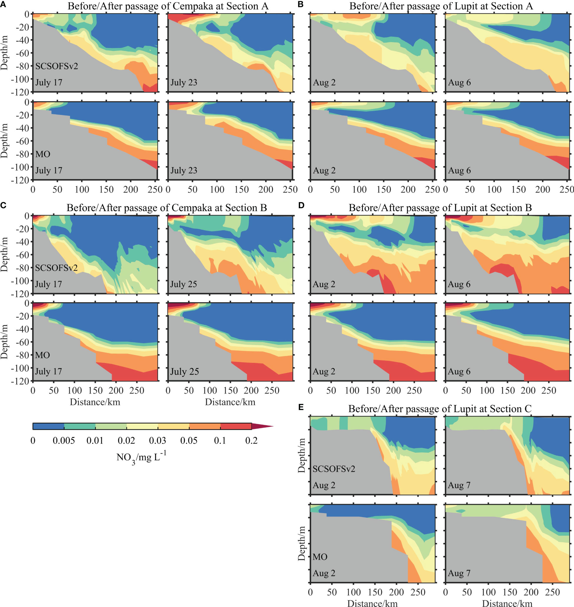
Figure 11 NO₃ variations at Section A (A, B), Section B (C, D), and Section C (E) on the continental shelf during before and after Cempaka and Lupit. Data provided by SCSOFSv2 or MO is labelled in the first map of each row and the date has been marked in each map.

During the Lupit period, NO₃ at each section changed significantly. Compared with August 2, the change in NO₃ was weaker in the coastal waters at Section A but showed a clear upward mixing to reduce the range of low NO₃ in the upper and middle layers on August 6 (Figure 11B). Surface NO₃ extended from the coast to the continental shelf, whereas the bottom NO₃ on the continental shelf was uplifted at Section B (Figure 11D). NO₃ crossing the Taiwan Bank at Section C increased from 0–0.02 mg L⁻¹ before Lupit to 0.01–0.03 mg L⁻¹ after Lupit (Figure 11E).

Different Chla bloom processes were generally discovered on the coastal waters and continental shelf (Zheng and Tang, 2007; Liu et al., 2013). Both Cempaka and Lupit brought heavy rainfall in coastal waters, consequently increasing the nutrient-carrying discharge. These extra nutrients stimulated the growth of phytoplankton with Chla bloom (Zhao et al., 2009; Herbeck et al., 2011). Previous studies pointed out that discharge contributes to Chla bloom in the estuary and nearshore waters, whereas its impact was relatively limited on the continental shelf (Song et al., 2011; Liu et al., 2013). However, both results from SCSOFSv2 and MO revealed that the high surface NO₃ extended from coastal waters to the continental shelf 50–150 km away from the coastline and was not completely connected with the high bottom NO₃ (Figure 11). Therefore, high surface NO₃ on the continental shelf diffuses from coastal waters, indicating that the nutrients brought by runoff discharge also contribute to surface Chla bloom on the continental shelf. In addition, nutrients are transported upward due to vertical mixing or upwelling caused by a typhoon leading to Chla bloom in the middle and upper layers of the outer continental shelf near the slope (Zheng and Tang, 2007; Zhao et al., 2009). It is worth noting that the bottom NO₃ in the Taiwan Bank is low before Lupit’s arrival. Previous observations confirmed that a typhoon passing the eastern Guangdong shelf strengthened the transport of cold bottom water from the slope to the nearshore (Pan et al., 2012). This means that nutrients are uplifted along the continental slope with the cold bottom water after a typhoon passes. Subsequently, NO₃ concentration increases in the water column through vertical mixing, consistent with the spread of SCSOFSv2 and MO NO₃ from the open sea to the slope at Section C (Figure 11E). Eventually, increased NO₃ supports Chla enhancement (Figure 10E).

4 Conclusion

Based on the data provided by SCSOFSv2, MO, and observations, this study focuses on the oceanic and ecological response to native typhoons Cempaka and Lupit, generated on the northern SCS continental shelf during July and August 2021. Both SCSOFSv2 and MO simulate SST cooling and Chla bloom induced by these two typhoons, with results that agree well with the observations.

In the PRE, correlation coefficients of temperature profiles between SCSOFSv2 and MO and the observations are 0.93 and 0.95 at 99% CL, and RMSEs are 1.24°C and 0.84°C, respectively. The MO simulation exhibits a lower error than SCSOFSv2. However, SCSOFSv2 Chla profiles in the PRE are better than MO compared to the observations, with a higher correlation coefficient and lower RMSE. By contrast, correlation coefficients between SCSOFSv2 (MO) SSTA and GHRSST anomalies are 0.85 and 0.86 (0.81 and 0.77) at 99% CL, and the RMSEs are is 0.28°C and 0.34°C (0.32°C and 0.37°C) during the Cempaka and Lupit periods, respectively. SCSOFSv2 SST changes are more consistent with the observations. The maximum SST drop simulated by SCSOFSv2 and MO is often 2–3 days earlier than the observation, and the cooling amplitude is larger than that of GHRSST. Surface Chla enhancement is the other significant feature besides the SST decrease after typhoons pass that can be reflected by the model and scarce satellite observations. The timing of Chla bloom simulated by SCSOFSv2 (MO) occurred after four (three) days and 2–3 (1–2) days with average Chla reaching a maximum three (two) days after typhoons passed the continental shelf and coastal waters, respectively. Cempaka- and Lupit-induced Chla blooms were higher than the average increase by 0.18 mg m⁻³ and also faster than the average time (4–5 days) on the SCS shelf.

Typhoon-induced vertical variations of Chla and NO₃ suggest different Chla bloom processes in coastal waters from the continental shelf. In the coastal waters, runoff discharge brings extra nutrients to stimulate phytoplankton growth with Chla bloom. The model results show that the discharge impact can extend from coastal waters to 50–150 km from the coastline. On the continental shelf, nutrients are uplifted due to the vertical mixing or upwelling caused by strong winds to support Chla enhancement in the upper and middle layers. In the Taiwan Bank, nutrients are transported from the open sea along the continental slope with the cold bottom water, then NO₃ in the water column is lifted through vertical mixing, eventually triggering Chla enhancement.

The SCSOFSv2 and MO results compared and evaluated with in situ and satellite observations reveal some differences in the SST and Chla timing and amplitude variations between SCOFSv2, MO, and observation on the continental shelf, especially in coastal waters. Some recommendations are provided as follows to further improve the performance of SCSOFS and MO during typhoon periods. First, both models should consider strong tides and waves to improve vertical mixing on the bottom and surface boundary layers in coastal waters. Second, both 1/12° and 1/30° horizontal resolutions are still insufficient to resolve the dynamic processes of the PRE. Hence, much higher-resolution coastal ocean models should be built using nesting or downscaling methods. Finally, observed data with much higher resolution should be obtained and assimilated into the numerical models.

Data availability statement

The raw data supporting the conclusions of this article will be made available by the authors, without undue reservation.

Author contributions

SG was responsible for data analysis and manuscript writing. XZ ran the physical part of SCSOFSv2 and designed the paper. XJ performed the biogeochemical part of SCSOFSv2 and analyzed model results. HJ and HW helped review, polish, and comment on the paper's contents. SZ and DW helped with analyzing the water samples. All authors revised the manuscript. All authors contributed to the article and approved the submitted version.

Funding

This work was supported and sponsored by the project of Southern Marine Science and Engineering Guangdong Laboratory (Zhuhai) (No. SML2020SP008), the National Natural Science Foundation of China (No. 42176029), and the Key Laboratory of Space Ocean Remote Sensing and Application (Ministry of Natural Resources) Open Research program (No. 202101001).

Acknowledgments

The authors appreciate the professional suggestions and comments from reviewers. We also thank all scientific researchers and crew for their contributions to the in situ observations during the Great Bay summer cruises in 2021 and 2022.

Conflict of interest

The authors declare that the research was conducted in the absence of any commercial or financial relationships that could be construed as a potential conflict of interest.

Publisher’s note

All claims expressed in this article are solely those of the authors and do not necessarily represent those of their affiliated organizations, or those of the publisher, the editors and the reviewers. Any product that may be evaluated in this article, or claim that may be made by its manufacturer, is not guaranteed or endorsed by the publisher.

Supplementary material

The Supplementary Material for this article can be found online at: https://www.frontiersin.org/articles/10.3389/fmars.2023.1175263/full#supplementary-material

References

Aumont O., Ethé C., Tagliabue A., Bopp L., Gehlen M. (2015). PISCES-v2: an ocean biogeochemical model for carbon and ecosystem studies. Geosci. Model. Dev. 8, 2465–2513. doi: 10.5194/gmd-8-2465-2015

CrossRef Full Text | Google Scholar

Bingham F. (2007). Physical response of the coastal ocean to hurricane Isabel near landfall. Ocean Sci. 3, 159–171. doi: 10.5194/os-3-159-2007

CrossRef Full Text | Google Scholar

Black W. J., Dickey T. D. (2008). Observations and analyses of upper ocean responses to tropical storms and hurricanes in the vicinity of Bermuda. J. Geophys. Res. Oceans 113, C08009. doi: 10.1029/2007JC004358

CrossRef Full Text | Google Scholar

Brasseur P., Verron J. (2006). The SEEK filter method for data assimilation in oceanography: a synthesis. Ocean Dynam. 56, 650–661. doi: 10.1007/s10236-006-0080-3

CrossRef Full Text | Google Scholar

Carton J. A., Chepurin G. A., Chen L. (2018). SODA3: a new ocean climate reanalysis. J. Clim. 31, 6967–6983. doi: 10.1175/JCLI-D-18-0149.1

CrossRef Full Text | Google Scholar

Chacko N. (2017). Chlorophyll bloom in response to tropical cyclone hudhud in the bay of Bengal: bio-argo subsurface observations. Pt. I: Oceanogr. Res. Papers 124, 66–72. doi: 10.1016/j.dsr.2017.04.010

CrossRef Full Text | Google Scholar

Chai F., Dugdale R. C., Peng T. H., Wilkerson F. P., Barber R. T. (2002). One-dimensional ecosystem model of the equatorial pacific upwelling system. part I: model development and silicon and nitrogen cycle. Deep Sea Res. II: Top. Stud. Oceanogr. 49, 2713–2745, 49, 2713-2745. doi: 10.1016/S0967-0645(02)00055-3

CrossRef Full Text | Google Scholar

Chang Y., Liao H. T., Lee M. A., Chan J. W., Shieh W. J., Lee K. T., et al. (2008). Multisatellite observation on upwelling after the passage of typhoon hai-tang in the southern East China Sea. Geophys. Res. Lett. 35, L03612. doi: 10.1029/2007GL032858

CrossRef Full Text | Google Scholar

Chen Y.-L. (2005). Spatial and seasonal variations of nitrate-based new production and primary production in the south China Sea. Deep Sea. Res. Pt. I: Oceanogr. Res. Papers 52, 319–340. doi: 10.1016/j.dsr.2004.11.001

CrossRef Full Text | Google Scholar

Chen Y.-L., Chen H.-Y., Jan S., Tuo S.-H. (2009). Phytoplankton productivity enhancement and assemblage change in the upstream kuroshio after typhoons. Mar. Ecol. Prog. Ser. 385, 111–126. doi: 10.3354/meps08053

CrossRef Full Text | Google Scholar

Chen D., He L., Liu F., Yin K. (2017). Effects of typhoon events on chlorophyll and carbon fixation in different regions of the East China Sea. Estuar. Coast. Shelf Sci. 194, 229–239. doi: 10.1016/j.ecss.2017.06.026

CrossRef Full Text | Google Scholar

Chen X., Pan D., Bai Y., He X., Arthur Chen C. T., Kang Y., et al. (2015). Estimation of typhoon-enhanced primary production in the south China Sea: a comparison with the Western north pacific. Cont. Shelf Res. 111, 286–293. doi: 10.1016/j.csr.2015.10.003

CrossRef Full Text | Google Scholar

Chen X. W., Qiu C. H., Zhang H., Liu D., Shi H., Ma Y. G., et al. (2022). Response to typhoons in coastal waters at jitimen in zhujiang river estuary. Oceanol. Et Limnol. Sinica. 53, 872–881. doi: 10.11693/hyhz20220100001(In Chinese)

CrossRef Full Text | Google Scholar

Chen Y., Tang D. (2012). Eddy-feature phytoplankton bloom induced by a tropical cyclone in the south China Sea. Int. J. Remote Sens. 33, 7444–7457. doi: 10.1080/01431161.2012.685976

CrossRef Full Text | Google Scholar

Donlon C., Robinson I., Casey K. S., Vazquez-Cuervo J., Armstrong E., Arino O., et al. (2007). The global ocean data assimilation experiment high-resolution Sea surface temperature pilot project. B. Am. Meteorol. Soc 88, 1197–1214. doi: 10.1175/bams-88-8-1197

CrossRef Full Text | Google Scholar

Farris A., Wimbush M. (1996). Wind-induced kuroshio intrusion into the south China Sea. J. Oceanogr. 52, 771–784. doi: 10.1007/BF02239465

CrossRef Full Text | Google Scholar

Feng Y., Huang J., Du Y., Balaguru K., Ma W., Feng Q., et al. (2022). Drivers of phytoplankton variability in and near the pearl river estuary, south China Sea during typhoon Hato, (2017): a numerical study. J. Geophys. Res. Biogeo. 127, e2022JG006924. doi: 10.1029/2022JG006924

CrossRef Full Text | Google Scholar

Guo L., Xiu P., Chai F., Xue H., Wang D., Sun J. (2017). Enhanced chlorophyll concentrations induced by kuroshio intrusion fronts in the northern south China Sea. Geophys. Res. Lett. 44, 11565–11572. doi: 10.1002/2017GL075336

CrossRef Full Text | Google Scholar

Herbeck L. S., Unger D., Krumme U., Liu S. M., Jennerjahn T. C. (2011). Typhoon-induced precipitation impact on nutrient and suspended matter deepdynamics of a tropical estuary affected by human activities in hainan, China. Estuar. Coast. Shelf Sci. 93, 375–388. doi: 10.1016/j.ecss.2011.05.004

CrossRef Full Text | Google Scholar

Hersbach H., Bell B., Berrisford P., Hirahara S., Horányi A., Muñoz Sabater J., et al. (2020). The ERA5 global reanalysis.Q. J. R. Meteor. Soc 146, 1999–2049. doi: 10.1002/qj.3803

CrossRef Full Text | Google Scholar

Hung C. C., Gong G. C., Chou W.-C., Chung C. C., Lee M.-A., Chang Y., et al. (2010). The effect of typhoon on particulate organic carbon flux in the southern East China Sea. Biogeosciences 7, 3007–3018. doi: 10.5194/bg-7-3007-2010

CrossRef Full Text | Google Scholar

Lai Q. Z., Wu L. G., Shie C. L. (2013). Sea Surface temperature response to typhoon Morakot, (2009) and the influence on its activity. J. Trop. Meteorol. 29, 221–234. doi: 10.3969/j.issn.1004-4965.2013.02.006(In Chinese)

CrossRef Full Text | Google Scholar

Leipper D. F. (1967). Observed ocean conditions and hurricane hild. J. Atmos. Sci. 24, 182–186. doi: 10.1175/1520-0469(1967)024<0182:OOCAHH>2.0.CO;2

CrossRef Full Text | Google Scholar

Lellouche J.-M., Greiner E., Le Galloudec O., Garric G., Regnier C., Drevillon M., et al. (2018). Recent updates to the Copernicus marine service global ocean monitoring and forecasting realtime1/12° high-resolution system. Ocean Sci. 14, 1093–1126. doi: 10.5194/os-14-1093-2018

CrossRef Full Text | Google Scholar

Lellouche J. M., Le Galloudec O., Drévillon M., Régnier C., Greiner E., Garric G., et al. (2013). Evaluation of global monitoring and forecasting systems at Mercator océan. Ocean Sci. 9, 57–81. doi: 10.5194/os-9-57-2013

CrossRef Full Text | Google Scholar

Li Y., Tang D. (2022). Tropical cyclone wind pump induced chlorophyll-a enhancement in the south China Sea: a comparison of the open sea and continental shelf. Front. Mar. Sci. 9. doi: 10.3389/fmars.2022.1039824

PubMed Abstract | CrossRef Full Text | Google Scholar

Liang X. H., Ge L. L. (2014). Analysis of impacts of typhoons on sea surface temperature of coastal region of jiangsu province. J. Aquac. 35, 37–42. doi: 10.3969/j.issn.1004-2091.2014.10.008. (In Chinese).

CrossRef Full Text | Google Scholar

Lin I., Liu W. T., Wu C. C., Chiang J. C. H., Sui C. H. (2003a). Satellite observations of modulation of surface winds by typhoon-induced upper ocean cooling. Geophys. Res. Lett. 30, 1131. doi: 10.1029/2002GL015674

CrossRef Full Text | Google Scholar

Lin I., Liu W. T., Wu C. C., Wong G. T. F., Hu C., Chen Z., et al. (2003b). New evidence for enhanced ocean primary production triggered by tropical cyclone. Geophys. Res. Lett. 30, 1718. doi: 10.1029/2003GL017141

CrossRef Full Text | Google Scholar

Liu H., Hu Z., Huang L., Huang H., Chen Z., Song X., et al. (2013). Biological response to typhoon in northern south China Sea: a case study of “Koppu”. Cont. Shelf Res. 68, 123–132. doi: 10.1016/j.csr.2013.08.009

CrossRef Full Text | Google Scholar

Liu Q., Zhang J., Huang Z., Huang N. (2010). The stable isotope geochemical characteristics of dissolved inorganic carbon in northern south China Sea. Chin. J. Geochem. 29, 287–292. doi: 10.1007/s11631-010-0458-2

CrossRef Full Text | Google Scholar

Lu X., Yu H., Ying M., Zhao B., Zhang S., Lin L., et al. (2021). Western North pacific tropical cyclone database created by the China meteorological administration. Adv. Atmos. Sci. 38, 690–699. doi: 10.1007/s00376-020-0211-7

CrossRef Full Text | Google Scholar

Madec G., Bourdallé-Badie R., Bouttier P. A., Bricaud C., Bruciaferri D., Calvert D., et al. (2017). NEMO ocean engine (Version v3.6), notes Du pôle de modélisation de l’institut Pierre-simon Laplace (IPSL) (Zenodo). doi: 10.5281/zenodo.1472492

CrossRef Full Text | Google Scholar

Mrvaljevic R. K., Black P. G., Centurioni L. R., Chang Y.-T., D’Asaro E. A., Jayne S. R., et al. (2013). Observations of the cold wake of typhoon Fanapi, (2010). Geophys. Res. Lett. 40, 316–321. doi: 10.1029/2012GL054282

CrossRef Full Text | Google Scholar

Nan F., Xue H., Chai F., Wang D., Yu F., Shi M., et al. (2013). Weakening of the kuroshio intrusion into the south China Sea over the past two decades. J. Clim. 26, 8097–8110. doi: 10.1175/jcli-d-12-00315.1

CrossRef Full Text | Google Scholar

Pan A., Guo X., Xu J., Huang J., Wan X. (2012). Responses of guangdong coastal upwelling to the summertime typhoons of 2006. Sci. China Earth Sci. 55, 495–506. doi: 10.1007/s11430-011-4321-z

CrossRef Full Text | Google Scholar

Price J. F., Morzel J., Niiler P. P. (2008). Warming of SST in the cool wake of a moving hurricane. J. Geophys. Res. Oceans 113, C07010. doi: 10.1029/2007JC004393

CrossRef Full Text | Google Scholar

Qiu D., Zhong Y., Chen Y., Tan Y., Song X., Huang L. (2019). Short-term phytoplankton dynamics during typhoon season in and near the pearl river estuary, south China Sea. J. Geophys. Res. Biogeo. 124, 274–292. doi: 10.1029/2018JG004672

CrossRef Full Text | Google Scholar

Qu T. (2000). Upper-layer circulation in the south China Sea. J. Phys. Oceanogr. 30, 1450–1460. doi: 10.1175/1520-0485(2000)030<1450:ULCITS>2.0.CO;2

CrossRef Full Text | Google Scholar

Roy Chowdhury R., Prasanna Kumar S., Chakraborty A. (2022). A study on the physical and biogeochemical responses of the bay of Bengal due to cyclone madi. J. Oper. Oceanogr. 15, 104–125. doi: 10.1080/1755876X.2020.1817659

CrossRef Full Text | Google Scholar

Saffir H. S. (1973). Hurricane wind and storm surge. Military Eng. 423, 4–5.

Google Scholar

Saha S., Moorthi S., Pan H.-L., Wu X., Wang J., Nadiga S., et al. (2010). The NCEP climate forecast system reanalysis. B. Am. Meteorol. Soc 91, 1015–1058. doi: 10.1175/jcli-d-12-00823.1

CrossRef Full Text | Google Scholar

Saha S., Moorthi S., Wu X., Wang J., Nadiga S., Tripp P., et al. (2014). The NCEP climate forecast system version 2. J. Clim. 27, 2185–2208. doi: 10.1175/jcli-d-12-00823.1

CrossRef Full Text | Google Scholar

Sathyendranath S., Brewin R. J. W., Brockmann C., Brotas V., Calton B., Chuprin A., et al. (2019). An ocean-colour time series for use in climate studies: the experience of the ocean-colour climate change initiative (OC-CCI). Sensors-Basel 19, 4285. doi: 10.3390/s19194285

PubMed Abstract | CrossRef Full Text | Google Scholar

Shibano R., Yamanaka Y., Okada N., Chuda T., Suzuki S. I., Niino H., et al. (2011). Responses of marine ecosystem to typhoon passages in the western subtropical north pacific. Geophys. Res. Lett. 38, L18608. doi: 10.1029/2011GL048717

CrossRef Full Text | Google Scholar

Simpson R. H. (1974). The hurricane disaster potential scale. Weatherwise 27, 169–186. doi: 10.1080/00431672.1974.9931702

CrossRef Full Text | Google Scholar

Song X., Huang L., Zhang J., Yin K., Liu S., Tan Y., et al. (2011). Chemometric study of spatial variations of environmental and ecological characteristics in the zhujiang river (Pearl river) estuary and adjacent waters. Aata Oceanol. Sin. 30, 60. doi: 10.1007/s13131-011-0137-0

CrossRef Full Text | Google Scholar

Subrahmanyam B., Rao K. H., Srinivasa Rao N., Murty V. S. N., Sharp R. J. (2002). Influence of a tropical cyclone on chlorophyll-a concentration in the Arabian Sea. Geophys. Res. Lett. 29, 22-1-22–4. doi: 10.1029/2002GL015892

CrossRef Full Text | Google Scholar

Sui Y., Sheng J., Tang D., Xing J. (2022). Study of storm-induced changes in circulation and temperature over the northern south China Sea during typhoon linfa. Cont. Shelf Res. 249, 104866. doi: 10.1016/j.csr.2022.104866

CrossRef Full Text | Google Scholar

Sun J., Oey L. Y. (2015). The influence of the ocean on typhoon Nuri, (2008). Monthly Weather Rev. 143 (11), 4493–4513. doi: 10.1175/MWR-D-15-0029.1

CrossRef Full Text | Google Scholar

Valente A., Sathyendranath S., Brotas V., Groom S., Grant M., Taberner M., et al. (2019). A compilation of global bio-optical in situ data for ocean-colour satellite applications – version two. Earth Syst. Sci. Data 11, 1037–1068. doi: 10.5194/essd-11-1037-2019

CrossRef Full Text | Google Scholar

Wang Y. (2020). Composite of typhoon-induced Sea surface temperature and chlorophyll-a responses in the south China Sea. J. Geophys. Res. Oceans 125, e2020JC016243. doi: 10.1029/2020JC016243

CrossRef Full Text | Google Scholar

Wang G., Su J., Ding Y., Chen D. (2007). Tropical cyclone genesis over the south China sea. J. Mar. Syst. 68, 318–326. doi: 10.1016/j.jmarsys.2006.12.002

CrossRef Full Text | Google Scholar

Wu R., Li C. (2018). Upper ocean response to the passage of two sequential typhoons. Deep Sea. Res. Pt. I: Oceanogr. Res. Papers 132, 68–79. doi: 10.1016/j.dsr.2017.12.006

CrossRef Full Text | Google Scholar

Wu Y., Platt T., Tang C. C. L., Sathyendranath S. (2007). Short-term changes in chlorophyll distribution in response to a moving storm: a modelling study. Mar. Ecol. Prog. Ser. 335, 57–68. doi: 10.3354/meps335057

CrossRef Full Text | Google Scholar

Wyrtki K. (1961). Scientific results of marine investigation of the south China Sea and gulf of Thailand. Naga Rep. 2, 37–38.

Google Scholar

Xie L. L., He C. F., Li M. M., Tian J. J., Jing Z. Y. (2017). Response of sea surface temperature to typhoon passages over the upwelling zone east of hainan island. Adv. Mar. Sci. 35, 8–19. doi: 10.3969/j.issn.1671-6647.2017.01.002(In Chinese)

CrossRef Full Text | Google Scholar

Xiu P., Chai F. (2014). Connections between physical, optical and biogeochemical processes in the pacific ocean. Prog. Oceanogr. 122, 30–53. doi: 10.1016/j.pocean.2013.11.008

CrossRef Full Text | Google Scholar

Yang Y. J., Sun L., Liu Q., Xian T., Fu Y. F. (2010). The biophysical responses of the upper ocean to the typhoons namtheun and malou in 2004. Int. J. Remote Sens. 31, 4559–4568. doi: 10.1080/01431161.2010.485140

CrossRef Full Text | Google Scholar

Yue X., Zhang B., Liu G., Li X., Zhang H., He Y. (2018). Upper ocean response to typhoon kalmaegi and sarika in the south China Sea from multiple-satellite observations and numerical simulations. Remote Sens. 10, 348. doi: 10.3390/rs10020348

CrossRef Full Text | Google Scholar

Zeng J. Y., Lin J. G., Yu Y., Chen Q. P., Yin S. Y. (2022). An analysis on the track and intensity characteristics and forecast deviation of typhoon 2109 “Lupit”. Mar. Forecasts 39, 10–24. doi: 10.11737/j.issn.1003-0239.2022.03.002(In Chinese)

CrossRef Full Text | Google Scholar

Zhang H., Wu R., Chen D., Liu X., He H., Tang Y., et al. (2018). Net modulation of upper ocean thermal structure by typhoon Kalmaegi, (2014). J. Geophys. Res. Oceans. 122, 7154–7171. doi: 10.1029/2018JC014119

CrossRef Full Text | Google Scholar

Zhang M., Zhu X., Ji X., Zhang A., Zheng J. (2023). Controlling factor analysis of oceanic surface pCO2 in the south China Sea using a three- dimensional high resolution biogeochemical model. Front. Mar. Sci. 10. doi: 10.3389/fmars.2023.1155979

CrossRef Full Text | Google Scholar

Zhao H. (1990). The evolution of the pearl river estuary. Beijing: Ocean Press, pp. 116–147.

Google Scholar

Zhao H., Tang D., Wang Y. (2008). Comparison of phytoplankton blooms triggered by two typhoons with different intensities and translation speeds in the south China Sea. Mar. Ecol. Prog. Ser. 365, 57–65. doi: 10.3354/meps07488

CrossRef Full Text | Google Scholar

Zhao H., Tang D., Wang D. (2009). Phytoplankton blooms near the pearl river estuary induced by typhoon nuri. J. Geophys. Res. Oceans 114, C12027. doi: 10.1029/2009JC005384

CrossRef Full Text | Google Scholar

Zheng G., Tang D. (2007). Offshore and nearshore chlorophyll increases induced by typhoon winds and subsequent terrestrial rainwater runoff. Mar. Ecol. Prog. Ser. 333, 61–74. doi: 10.3354/meps333061

CrossRef Full Text | Google Scholar

Zhu X., Wang H., Liu G., Régnier C., Kuang X., Wang D., et al. (2016). Comparison and validation of global and regional ocean forecasting systems for the south China Sea. Nat. Hazards Earth Syst. Sci. 16, 1639–1655. doi: 10.5194/nhess-16-1639-2016

CrossRef Full Text | Google Scholar

Zhu X., Zu Z., Ren S., Zhang M., Zhang Y., Wang H., et al. (2022). Improvements in the regional south China Sea operational oceanography forecasting system (SCSOFSv2). Geosci. Model. Dev. 15, 995–1015. doi: 10.5194/gmd-15-995-2022

CrossRef Full Text | Google Scholar