Estimating thermohaline structures in the tropical Indian Ocean from surface parameters using an improved CNN model

1 Introduction

Ocean temperature and salinity are two of the most important parameters of seawater, playing an important role in regulating the transfer of heat (Johnson and Lyman, 2020), freshwater (Hall et al., 2008), and carbon (Smith et al., 2009) between the ocean and atmosphere (Watson et al., 2020). Changes in ocean temperature and salinity have significant impacts on ocean circulation, marine ecosystems, and the Earth’s climate system (Levitus et al., 2001; Sprintall et al., 2014). Accurately estimating the ocean subsurface thermal structure (OSTS) and ocean subsurface salinity structure (OSSS) is therefore important for understanding ocean dynamics, climate variability and predicting future climate scenarios. The tropical Indian Ocean is an important region for studying climate change as it has a significant impact on the regional and global climate (Luo et al., 2012; Cai et al., 2021). The ocean thermohaline structure in the tropical Indian Ocean exerts a significant influence on ocean circulation, climate variability and hydrological cycle by affecting the Earth’s energy budget, evaporation, and precipitation processes (Trenberth and Caron, 2001; Bao et al., 2019). Therefore, accurate estimation of the thermohaline structure in the tropical Indian Ocean is important for predicting the regional and global impacts of climate change on marine ecosystems, ocean circulation, and weather patterns (Schott et al., 2009; Ateweberhan and McClanahan, 2010).

The estimation of the OSTS and OSSS in the tropical Indian Ocean has traditionally relied on numerical simulation, data assimilation, and dynamical modeling techniques (Rao and Sivakumar, 2003; Liu et al., 2005; Rahaman et al., 2014; Yan et al., 2015). Although these traditional methods have achieved some successes, they are computationally intensive and require significant resources due to the complexity of the thermodynamic processes governed by a set of equations. Thus, an accurate and efficient approach to estimate OSTS and OSSS using acceptable computational resources is essential and remains an active research area.

Recent advances in remote sensing technology have brought about a revolution in ocean observations, providing continuous and widespread sampling of some sea surface parameters, such as sea surface salinity (SSS), sea surface height (SSH), and sea surface temperature (SST). Some earlier studies have demonstrated that many oceanic subsurface phenomena can be retrieved from surface manifestations using satellite observations, motivating exploration of the potential for estimating OSTS and OSSS from sea surface data (Khedouri et al., 1983; Fiedler, 1988; Ali et al., 2004; Klemas and Yan, 2014). Various approaches have been employed, such as statistical relationships (Khedouri et al., 1983; Yan et al., 2020), linear and geographically weighted regression models (Guinehut et al., 2012), empirical orthogonal functions (DeWitt, 1987; Maes and Behringer, 2000), and parametric models (Chu et al., 2000). For example, Maes and Behringer (2000) used the empirical orthogonal function (EOF) methodology to reconstruct subsurface salinity structure by utilizing sea level anomaly and SST data. Watts et al. (2001) utilized a gravest empirical mode (GEM) to reconstruct the temperature and salinity structures at various depths in the southern Australian region. This method has also been utilized in the Southern Ocean (Meijers et al., 2011). Guinehut et al. (2012) employed a linear regression model to reconstruct global temperature and salinity fields using sea surface data and in situ measurements with enhanced resolution. Despite their success, each method has its strengths and limitations. Therefore, researchers continue to explore new and innovative ways to retrieve the ocean interior structure using sea surface data.

Recently, the application of machine learning techniques in the ocean and atmosphere has received widespread attention, providing valuable insights to understand the intricate physical and dynamic processes between the ocean and the atmosphere (Reichstein et al., 2019). Among the various applications of machine learning, the estimation of the OSTS and OSSS has emerged as a prominent research area. In this regard, extensive efforts have been made to reconstruct ocean interior structures using machine learning techniques. For example, Ali et al. (2004) proposed a novel approach utilizing artificial neural networks (ANN) to reconstruct the temperature structure from sea surface data, including SSS, SST, net radiation, wind stress, and net heat flux. Wu et al. (2012) combined the self-organizing map neural network (SOM) algorithm with multiple satellite measurements to estimate subsurface temperature structure in the North Atlantic, showing that their model outperformed traditional methods and highlighting the potential of machine learning techniques in oceanography. Bao et al. (2019) proposed a generalized regression neural network with the fruit fly optimization algorithm (FOAGRNN) to reconstruct the three-dimensional salinity field in the Pacific Ocean via sea surface salinity data. Su et al. (2015; 2018a; 2018b, and 2021) successfully estimated OSTS using machine learning approaches such as support vector machine (SVM), Random Forest, light gradient boosting machine (LightGBM) and CNN. Meng et al. (2021) developed a CNN based deep neural network model to reconstruct the subsurface temperature anomalies and subsurface salinity anomalies in the Pacific Ocean and simultaneously enhance their resolution. Most recently, Pauthenet et al. (2022) presented a novel method for estimating the temperature and salinity structures in the Gulf Stream in combination with physical constraints.

While machine learning has emerged as a valuable tool for estimating ocean structure from sea surface data, pure machine learning models treat all input features equally, regardless of their relevance to the task at hand. This may result in the inclusion of irrelevant or noisy features, leading to a decrease in the model’s overall accuracy. Furthermore, these models may struggle to capture complex patterns or relationships in large or high-dimensional datasets. Recently, Li et al. (2022) demonstrated that the integration of various attention mechanisms into current deep learning-based ocean remote sensing models is a promising direction for the design and advancement of such models. Other studies have also incorporated the attention mechanism in their approach to ocean remote sensing processing. For example, Xie et al. (2022) utilized a combination of the U-net deep learning model and the attention mechanism to reconstruct a high-resolution subsurface temperature field in the South China Sea from satellite observations. The results revealed that the U-net model with the attention mechanism achieved superior performance compared to the pure U-net model, XGBoost machine learning model, and classical multiple linear regression model with the same inputs. In this study, we propose a novel model based on the Convolutional Block Attention Module-Convolutional Neural Network (CBAM-CNN) to estimate the OSTS and OSSS in the tropical Indian Ocean using satellite observations.

The rest of the study is organized as follows: Section 2 describes the data and methods, Section 3 presents the results, and Section 4 provides a summary and discussion.

2 Data and methods

2.1 Data

In this study, we use a range of sea surface data obtained from satellite observations to simultaneously estimate the OSTS and OSSS in the tropical Indian Ocean. Based on previous studies and analyses, we select SST, SSS, SSHA, and sea surface wind (SSW), which is separated into the eastward component sea surface wind (ESSW) and the northward component sea surface wind (NSSW), in combination with geographic information such as longitude (LON) and latitude (LAT), as independent input variables for the model (Qi et al., 2022). The SST data are obtained from the National Oceanic and Atmospheric Administration (NOAA), which combines AMSR, AVHRR, and in-situ observations with a spatial resolution of 1° latitude × 1° longitude (Reynolds et al., 2002). We also obtain SSS data from the Soil Moisture and Ocean Salinity (SMOS) Level-3 SSS product with a spatial resolution of 0.25° latitude × 0.25° longitude (Boutin et al., 2018), and SSHA data from the Archiving, Validation, and Interpretation of Satellite Oceanographic (AVISO) data center with a spatial resolution of 0.25° latitude × 0.25° longitude (Hauser et al., 2020). Additionally, we utilize SSW data from the Cross-Calibrated Multi-Platform (CCMP) product, which has a high-resolution of 0.25° latitude × 0.25° longitude (Atlas et al., 2011). To train and evaluate the performance of the models, we also utilize the Roemmich-Gilson Argo Climatology (RG-Argo) gridded data, with a horizontal resolution of 1° × 1°, and covers the period from January 2004 to the present (Roemmich and Gilson, 2009).

To ensure consistency and accuracy in the model, we process all the data into monthly averages, and interpolate them onto a grid with a resolution of 1° latitude × 1° longitude, with the same temporal and spatial coverage of the tropical Indian Ocean (35°E–120°E and 30°S–30°N). Any data points with missing parameters within the tropical Indian Ocean are excluded. Additionally, to expedite model convergence during the training process, all remote sensing data and Argo measurements are normalized by utilizing the data’s mean and standard deviation before training. Table 1 provides a summary of the data used in this study.

TABLE 1

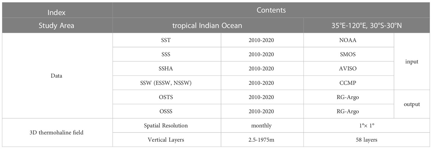
Table 1 Summary of data used in this study.

2.2 Methods

Recently, more and more deep learning models has used the attention mechanism, and it has also been an important development trend to add various attention mechanisms to deep learning models on ocean remote sensing (Li et al., 2022). In this study, we present an improved CNN model that incorporates the Convolutional Block Attention Module (CBAM) into the standard CNN architecture. The details of models used in this study are described in the following sections.

2.2.1 CNN and CBAM

CNN is a deep learning algorithm that has been extensively used in a variety of fields. In the geoscience community, CNN has gained widespread attention and has been successful in several applications (Ham et al., 2019; Meng et al., 2021). One of the key advantages of CNN is its ability to consider the spatial relationship between input data, making it particularly well-suited for geospatial data (Bolton and Zanna, 2019; Zheng et al., 2020). The ability of CNN to share weights also allows for efficient processing of high-dimensional data and automated feature extraction, making it a useful tool for estimating OSTS and OSSS accurately. However, the complex architecture of CNN can also lead to slow model parameter updates and difficulty in capturing the relationship between global and local information. A schematic of the CNN model used in this study is presented in Figure 1A.

FIGURE 1

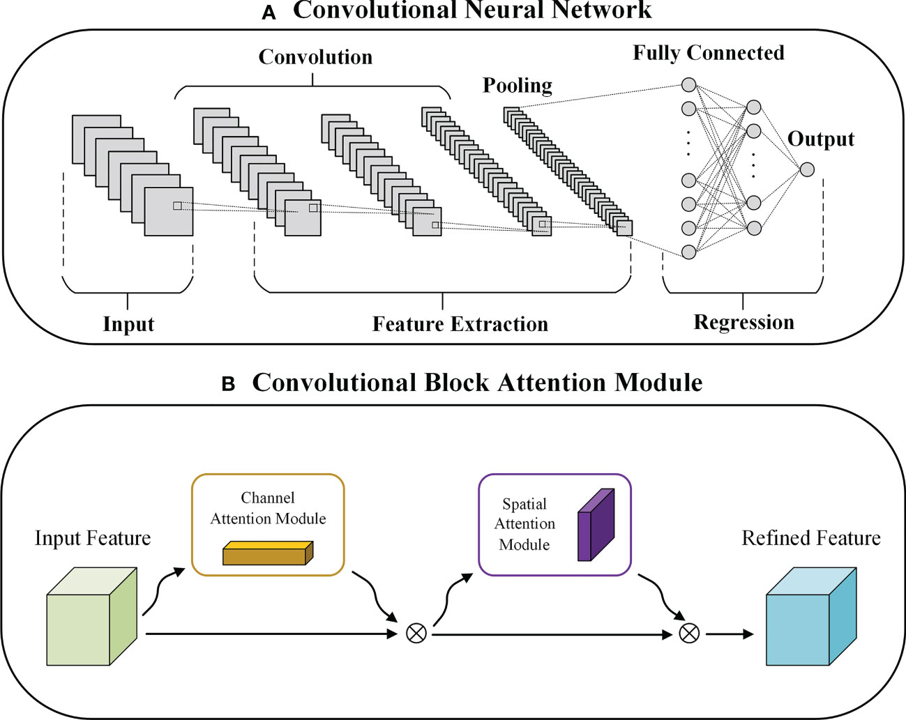
Figure 1 Structure of (A) CNN model and (B) CBAM module.

CBAM is a powerful attention mechanism that can enhance the performance of CNNs in computer vision tasks. It was developed by Woo et al. (2018), which consists of two modules, the Channel Attention Module (CAM) and the Spatial Attention Module (SAM) and can extract feature information from both the spatial and channel dimensions of the input data. As a lightweight architecture, CBAM can be seamlessly integrated into CNN-based models, making it an attractive option for improving the performance of deep learning models. In Figure 1B, the CBAM module is depicted, demonstrating its ability to enhance the performance of the CNN model.

2.2.2 CBAM-CNN

The CBAM-CNN model is an improved model of the CNN model, specifically designed to enhance the accuracy of estimating OSTS and OSSS from ocean surface parameters. By incorporating both the CAM and SAM, the CBAM-CNN model is capable of assigning weights to sea surface parameters along the channel and spatial dimensions, thus enabling it to focus its attention on key variables and informative features while excluding irrelevant factors. This attention mechanism significantly improves the model’s accuracy in estimating OSTS and OSSS and enhances its ability to generalize. The sequential utilization of CAM and SAM in the CBAM-CNN model allows for the efficient extraction of spatial and channel-wise feature information, leading to more accurate predictions. As shown in Figure 2, the CBAM-CNN model is composed of convolutional layers, a CBAM module, fully connected layers, an activation layer, and a global average pooling layer. The CBAM module is inserted after the convolutional and activation layers, and the Exponential Linear Unit (ELU) is used as the activation function, improving the model’s robustness and convergence speed by reducing the vanishing gradient effect (Clevert et al., 2015). To prevent overfitting, as well as exploding or vanishing gradients, we use Batch Normalization (BN) and Dropout algorithms after the convolutional and fully connected layers. We also employ the early stopping algorithm, which selects the best-performing model on the validation dataset, to prevent overfitting during training. Additionally, to optimize the training process, we include a global average pooling layer to reduce computational complexity.

FIGURE 2

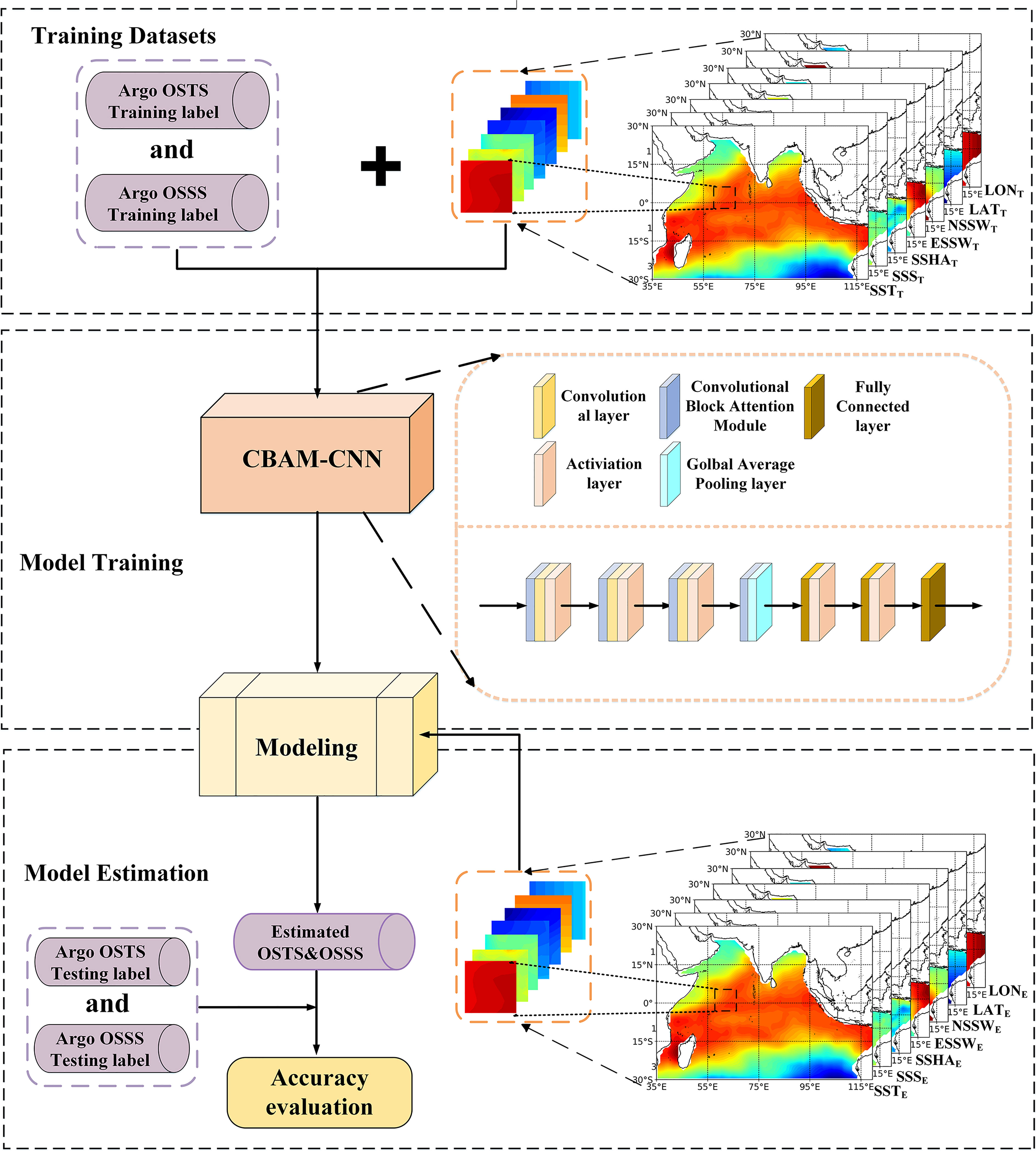
Figure 2 Flowchart of the CBAM-CNN model for estimating ocean subsurface thermohaline structure in the tropical Indian Ocean.

The CBAM-CNN model developed in this study consists of two primary steps for estimating the OSTS and OSSS in the tropical Indian Ocean. Firstly, we select the ocean surface parameters, including SST, SSS, SSHA, SSW, and geographic information (LON and LAT) as input data for the CBAM-CNN model, while the Argo data are used as training and testing labels. Secondly, we train and evaluate the model using the selected input and label data. Specifically, we input the training data from January 2010 through December 2019 into the CBAM-CNN model and randomly select 80% of the data for training and the remaining 20% for validation. Finally, we evaluate the performance of the CBAM-CNN model using data from 2020, based on the root mean square error (RMSE), normalized root mean square error (NRMSE), and determination coefficient (R²). Here, the RMSE is used as a metric to quantify the discrepancy between the predicted and observed values. It is calculated by taking the square root of the average of the squared differences between the predicted and observed values. The model’s performance is evaluated to determine its ability to accurately estimate OSTS and OSSS in the tropical Indian Ocean.

Optimizing the model parameters is a critical step in machine learning, as it directly impacts the performance of the models. In this study, we utilize the random search method to obtain the optimal combination of parameters for our models. The best combination of parameters for our models is presented in Table 2, which details the optimal values of hyperparameters for the CBAM-CNN model.

TABLE 2

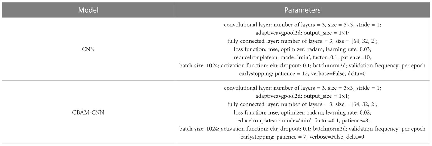
Table 2 Optimal combination of parameters of CBAM-CNN and CNN.

3 Results

3.1 Validation of satellite-derived SST and SSS

To ensure accurate predictions of OSTS and OSSS in the tropical Indian Ocean, it is essential to evaluate the accuracy of input data to machine learning models. Previous studies have highlighted the importance of SST and SSS for OSTS and OSSS estimation (Ali et al., 2004; Pauthenet et al., 2022). Therefore, in this study, we compare them to Argo-observed data. Figure 3 presents a spatial comparison of long-term annual mean of satellite-derived data and Argo-observed data. The satellite-derived data’s spatial distribution is highly consistent with the Argo-observed data in terms of both overall pattern and main features. For example, both the Argo data and satellite-derived data show that a thermal ridge run along the equator up to 60°E and thereafter sloping southwestwards west of 60°E. The northern tropical Indian Ocean has higher SSTs than the southern tropical Indian Ocean. Argo data identifies a region of high SSTs in the southwest region of the Arabian Sea, and satellite-derived SST reproduces this feature. The SST discrepancies are mainly between -0.1 and 0.25°C (Figure 3C). Similarly, the SSS data from satellite and Argo observations display good consistency and similar spatial distribution features. They both indicate that the maximum SSS (>36 psu) occurs in the northern Arabian Sea, while the minimum (<33 psu) occurs in the Bay of Bengal. The SSS discrepancies are concentrated between -0.1 psu and 0.1 psu (Figure 3F). Although slight discrepancies exist, these comparisons confirm the accuracy of satellite remote sensing data and provide reliable support for further research.

FIGURE 3

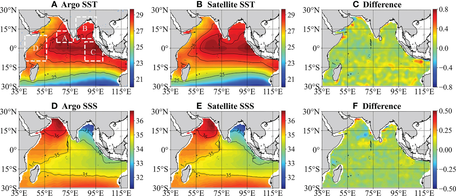
Figure 3 Long-term annual mean SST and SSS from Argo (left panel: A, D) and satellite observations (middle panel: B, E), as well as the differences between the two (right panel: C, F) in the tropical Indian Ocean from January 2010 to December 2020. Boxes (A–D) represent four boxes used in this study. Box A (64.5°E~76.5°E and 4.5°N~13.5°N), Box B (79.5°E~95.5°E and 7.5°N~23.5°N), Box C (87°E~105°E and 10°S~5°N), and Box D (40°E~55°E and 10°S~10°N).

3.2 Comparison of the CBAM-CNN model with CNN model

In this section, we compare the performance of the CBAM-CNN model and CNN model for estimating the OSTS and OSSS in the tropical Indian Ocean using data from 2020. Figure 4 illustrates the vertical distributions of RMSE and R² for both models. The results indicate that the overall RMSE values for OSTS increase from the surface to a maximum value near 100 m depth, before decreasing with depth. Conversely, the overall R² values show an opposite trend, decreasing from the surface to 100 m depth before gradually increasing and reaching their maximum around 1200 m before decreasing again. The same pattern is observed for OSSS, where the RMSE initially increase and then decrease, and the R² first decrease and then rapidly increase before reaching its maximum around 1200 m and then gradually decreasing with depth. The results indicate that the accuracy of OSTS and OSSS estimation decreases at depths of approximately 100-150 m, possibly due to the presence of a thermocline layer, which makes it challenging to accurately estimate the OSTS and OSSS. In contrast, it is evident that the CBAM-CNN model outperforms the original CNN model, as demonstrated by the smaller RMSE and larger R² values (as shown in Figure 4).

FIGURE 4

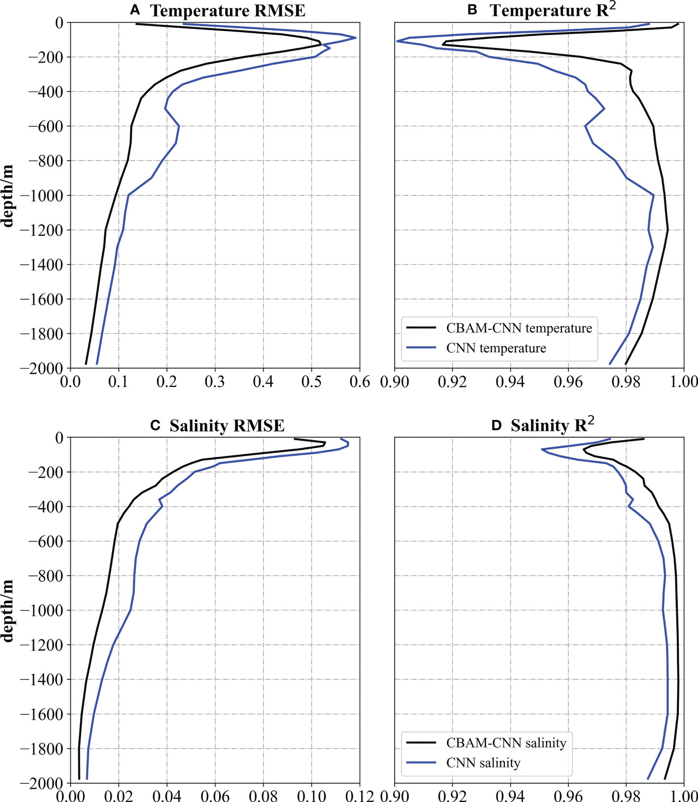
Figure 4 Comparison of the CBAM-CNN model (black line) with CNN model (blue line) for OSTS and OSSS estimation at different depths based on (A, C) RMSE (°C) and (B, D) R² in 2020.

To further compare the performance of the CBAM-CNN model and CNN model for estimating OSTS and SSS, we analyze the vertical averaged RMSE of the estimated temperature and salinity profiles in the tropical Indian Ocean. Figure 5 displays the spatial distribution of RMSE, and reveals that the CBAM-CNN model outperforms the CNN model. For example, in the southern tropical Indian Ocean (south of 15°S) and in the southeastern Arabian Sea, the RMSE of OSTS estimated by the CBAM-CNN model is significantly lower than that of the CNN model (Figures 5A, B). Likewise, the RMSE of OSSS estimated by the CBAM-CNN model is generally lower than that of the CNN model across most regions. For example, in the northern Bay of Bengal, the CBAM-CNN model demonstrates superior performance compared to the CNN model, as evidenced by the RMSE of OSSS estimates (Figures 5C, D). This superiority of the CBAM-CNN model can be attributed to its enhanced ability to capture spatial attention and represent complex oceanographic processes. Overall, these results demonstrate the CBAM-CNN model’s capabilities in accurately estimating OSTS and OSSS in the tropical Indian Ocean.

FIGURE 5

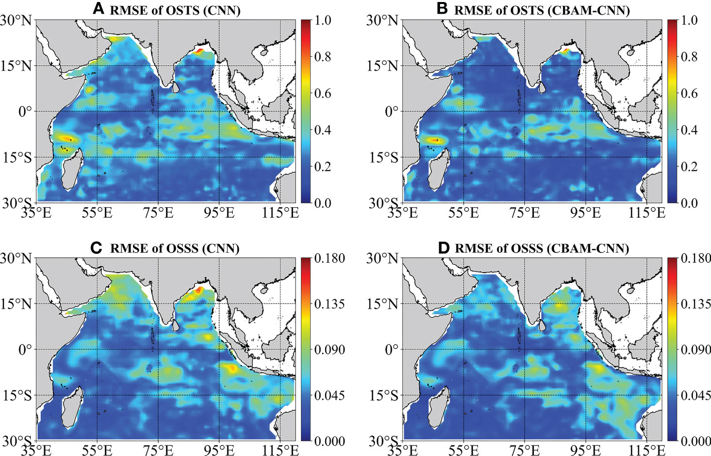
Figure 5 Spatial distribution of vertical averaged temperature and salinity RMSE in 2020: (A) CNN and (B) CBAM-CNN models for OSTS, (C) CNN and (D) CBAM-CNN models for OSSS.

3.3 Evaluation of the CBAM-CNN model

In this section, we conduct a comprehensive evaluation of the performance of the CBAM-CNN model from multiple perspectives. The annual average OSTS and OSSS estimated by the CBAM-CNN model at six different depths (50 m, 100 m, 500 m, 1000 m, 1500 m, and 1900 m) in 2020 are shown in Figures 6, 7. The differences between the Argo data and the CBAM-CNN estimated data (the difference between Argo and CBAM-CNN model data) are used to evaluate the performance of the CBAM-CNN model. Figure 6 shows the spatial distribution of the CBAM-CNN estimated OSTS and demonstrates a high level of agreement with the Argo-derived OSTS at different depths. The CBAM-CNN model accurately captures prominent temperature features using sea surface data in the tropical Indian Ocean. At 50 m depth, both the CBAM-CNN model and Argo data reveal a higher temperature in the northern tropical Indian Ocean than in the southern region, with the highest temperature observed in the equatorial eastern Indian Ocean. The temperature gradually decreases from the equator towards the south, and a prominent temperature front appears near 20°S. The temperature differences in most regions range from -0.5°C to 0.5°C (Figure 6C). The CBAM-CNN model also demonstrates good agreement with Argo observations for OSTS estimation at a depth of 100 m. However, the differences at this depth are slightly larger than those at 50 m, ranging from −0.6°C to 0.6°C. Notably, relatively large differences are observed in the region between the equator and 10°S, which may be attributed to the presence of the thermocline layer and the impact of upwelling. As the depth increases, the temperature becomes more stable, and the differences between the temperature values derived from Argo data and the CBAM-CNN model estimation below 500 m are relatively small, ranging from -0.1°C to 0.1°C. Overall, these results demonstrate the high accuracy of the CBAM-CNN model in estimating OSTS in the tropical Indian Ocean.

FIGURE 6

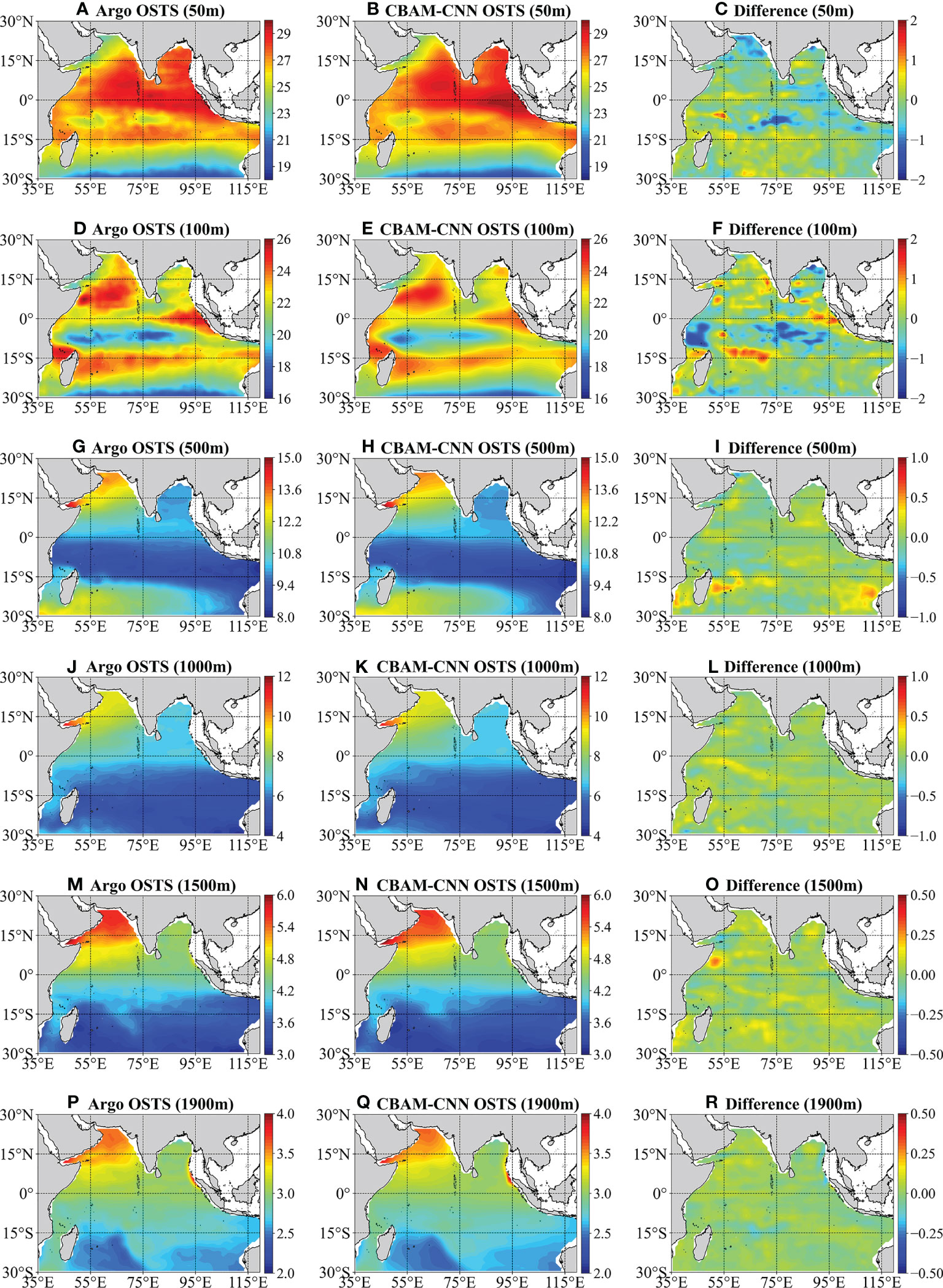
Figure 6 Annual average OSTS from Argo observation (left panel) and CBAM-CNN estimation (middle panel) and their differences (Argo minus CBAM-CNN, right panel) at different depths (50 m, 100 m, 500 m, 1000 m, 1500 m, 1900 m) in 2020.

FIGURE 7

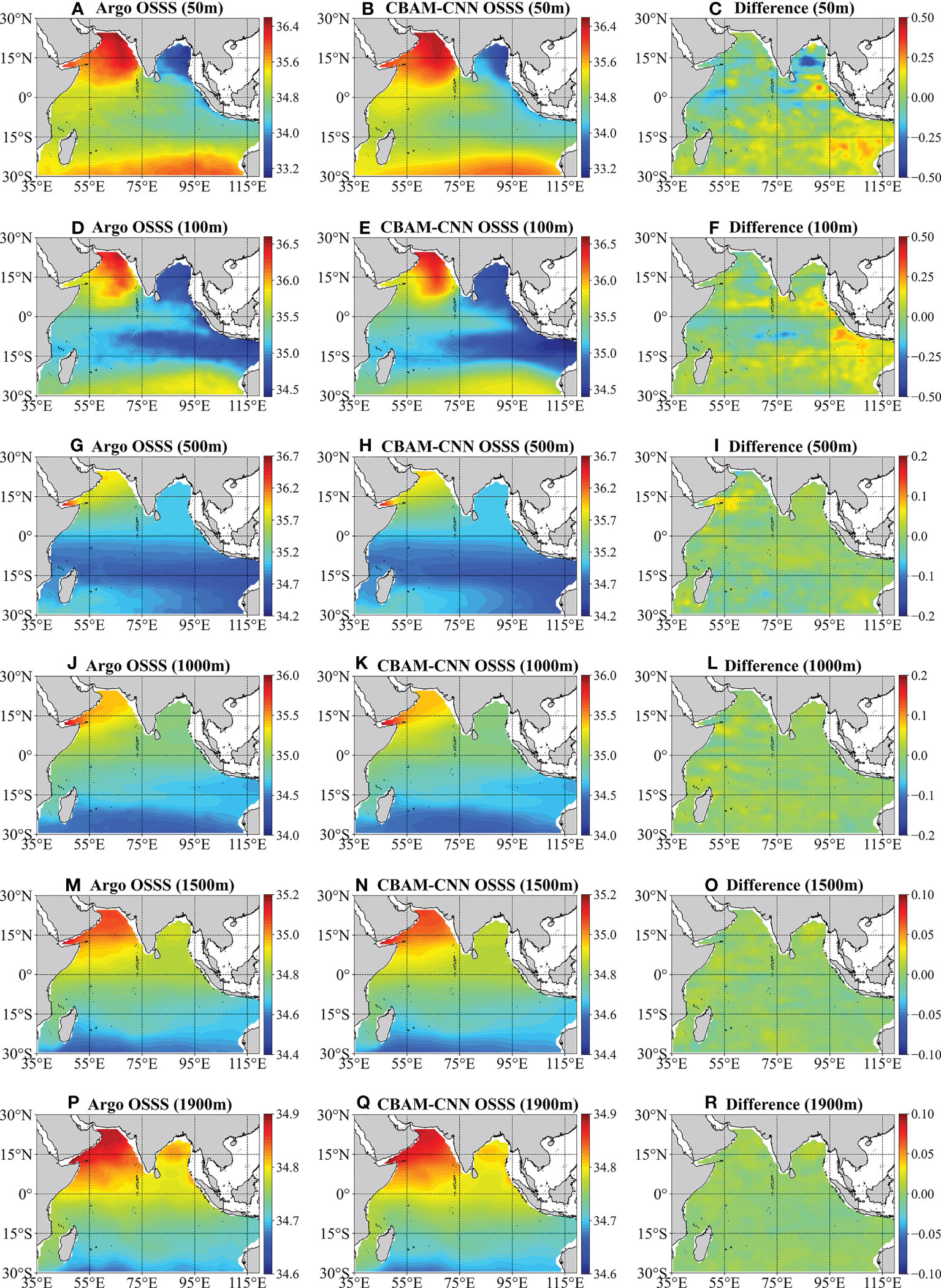
Figure 7 Same as Figure 6, but for OSSS.

Likewise, the CBAM-CNN model also exhibits good consistency with Argo observations for OSSS estimation, effectively reproducing the distribution characteristics of OSSS without significant differences observed between the CBAM-CNN estimated OSSS and the Argo-derived OSSS (Figure 7). In the upper ocean (50 m and 100 m), the differences of salinity in most regions range from -0.24 psu to 0.24 psu. As the depth increases, the OSSS becomes more stable, with the differences between the CBAM-CNN model estimated salinity and Argo-derived salinity are lower than 0.1 psu. These results confirm the effectiveness of the CBAM-CNN model in estimating OSSS in the tropical Indian Ocean. A more comprehensive evaluation of the CBAM-CNN model is presented in the subsequent section.

To comprehensively evaluate the performance of the CBAM-CNN model, we compare its estimated temperature and salinity profiles with Argo profiles in 2020 in four representative regions: Boxes A, B, C, and D (Figures 8, 9). Taking into consideration the spatial distribution characteristics of temperature and salinity, we carefully select four representative boxes, Boxes A, B, C, and D, as shown in Figure 3A. Box A (64.5°E~76.5°E and 4.5°N~ 13.5°N) is located in the SEAS area that have considerable influence on the marine ecosystem, Indian monsoon, and climate variability, Box B (79.5°E~95.5°E and 7.5°N~23.5°N) is situated in the BOB region where it has high rainfall and cyclonic activity, Box C (87°E~105°E and 10°S~5°N) is situated in the EEIO, which is influenced by the Walker circulation and the Indian Ocean Dipole (IOD), and Box D (40°E~55°E and 10°S~10°N) is located in the western equatorial Indian Ocean (WEIO), which is the western pole of the IOD and is an upwelling region where the Indian Ocean monsoon prevails. This selection allows us to comprehensively evaluate the performance of the CBAM-CNN model in capturing the complex features of temperature and salinity in these regions.

FIGURE 8

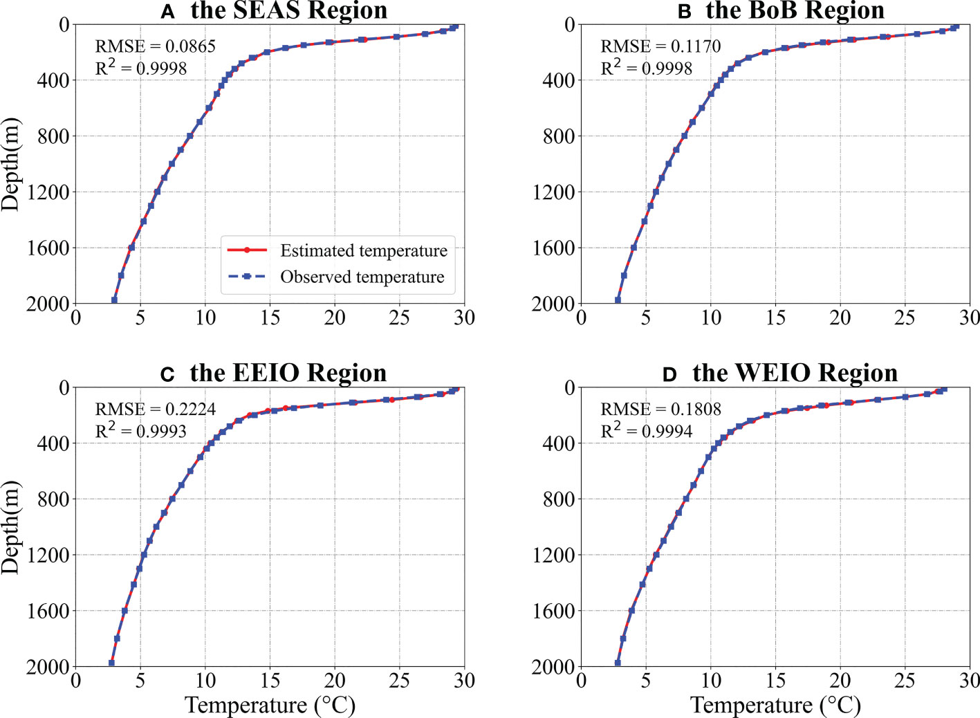
Figure 8 Comparison of area-averaged temperature profiles [(A–D) Boxes A-D] at different depths by the CBAM-CNN model estimated (red dotted line) and Argo observed (blue star line).

FIGURE 9

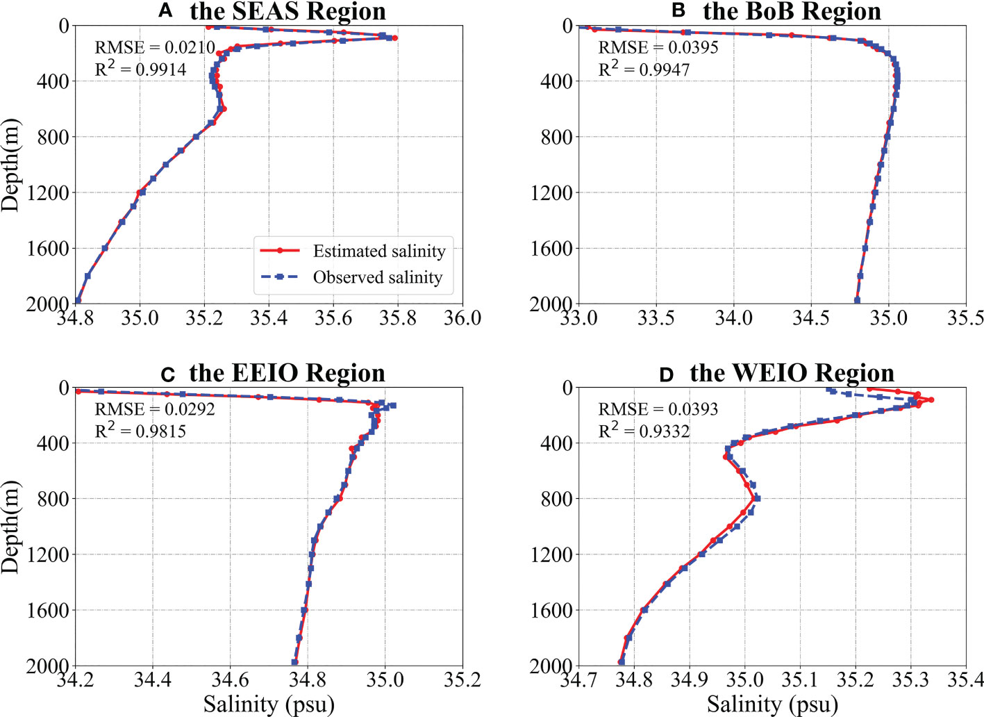
Figure 9 Same as Figure 8, but for salinity.

The comparison of estimated temperature profiles by the CBAM-CNN model with the Argo profiles in these four regions shows that the estimated temperature profiles are in good agreement with the Argo profiles (Figure 8). The vertical mean RMSE and R² values for each box are 0.0865°C and 0.9998 for Box A, 0.1170°C and 0.9998 for Box B, 0.2224°C and 0.9993 for Box C, and 0.1808°C and 0.9994 for Box D, respectively. These results suggest that the CBAM-CNN model can accurately reconstructs the vertical temperature profiles compared to the Argo observation data. Moreover, the CBAM-CNN model exhibits excellent performance in estimating OSSS (Figure 9). For example, the salinity profiles derived from Argo observations show two maxima in the WEIO, which the CBAM-CNN model accurately captures. The RMSE values between the Argo observations and the CBAM-CNN model are less than 0.04 psu, while the R² values exceed 0.93. These findings emphasize the CBAM-CNN model’s ability to reproduce the temperature and salinity profiles with high accuracy compared to the Argo observations.

As discussed above, the CBAM-CNN model demonstrates strong performance in estimating annual mean OSTS and OSSS in the tropical Indian Ocean. However, it remains unclear how well the model performs in different seasons. To address this question, we conduct a quantitative evaluation of the model’s accuracy in estimating OSTS and OSSS across seasons, specifically February, May, August, and November of 2020 representing winter, spring, summer, and autumn respectively. Firstly, we present correlation density scatterplots between the CBAM-CNN estimated temperature (salinity) and the Argo measured temperature (salinity) in different seasons, as depicted in Figure 10 (Figure 11). The plots illustrate that most data points are evenly distributed along the equal value lines, indicating a strong correlation between the estimated and observed OSTS and OSSS in the tropical Indian Ocean. Moreover, the RMSE and R² values between the Argo-observed temperature (salinity) and the CBAM-CNN estimated temperature (salinity) are calculated, with values of 0.5707°C (0.0823 psu) and 0.9948 (0.9613) in February, 0.5506°C (0.0818 psu) and 0.9952 (0.9620) in May, 0.5546°C (0.0760 psu) and 0.9946 (0.9677) in August, and 0.5424°C (0.0811 psu) and 0.9950 (0.9633) in November. These results indicate that the CBAM-CNN model has reliable and accurate seasonal performance in estimating OSTS and OSSS in the tropical Indian Ocean.

FIGURE 10

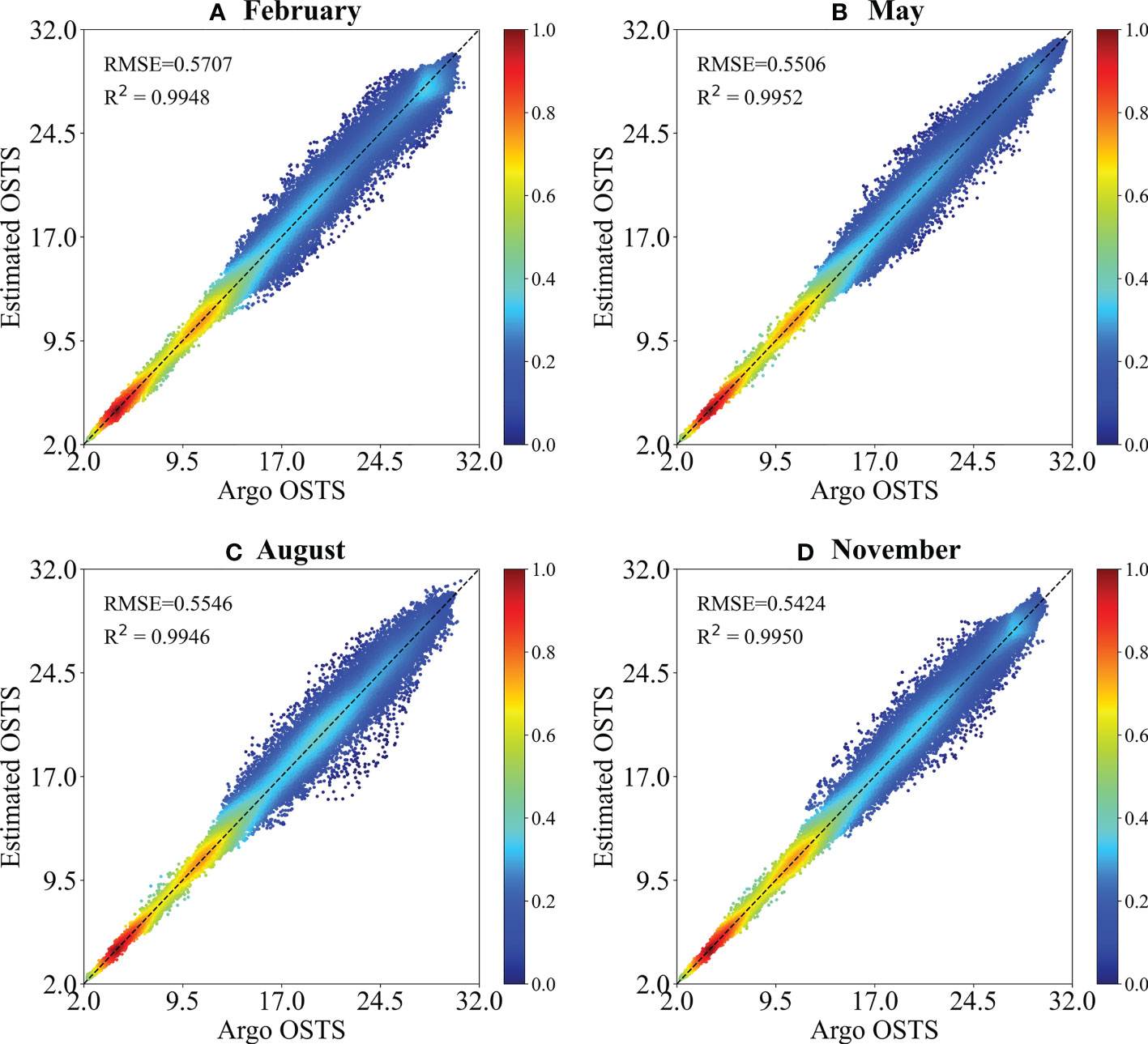
Figure 10 Scatter plots of temperature from Argo observation and CBAM-CNN model estimation in (A) February, (B) May, (C) August, and (D) November in 2020.

FIGURE 11

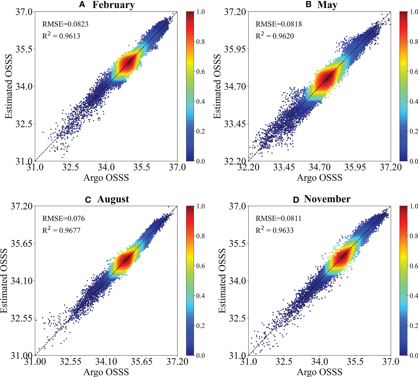
Figure 11 Same as Figure 10, but for salinity.

We also evaluate the seasonal performance of the CBAM-CNN model at different depths. To make the model accuracy at different depths comparable, we normalize the RMSE values (NRMSE) by dividing the RMSE with the standard deviation of the Argo temperature and salinity values at that depth. The vertical distribution of the NRMSE and R² at different depths for different seasons is presented in Figure 12. The results indicate that the CBAM-CNN model performs well overall. For both OSTS and OSSS estimation, the NRMSE values show an increasing trend followed by a decreasing trend, and then increasing again with depth. The maximum NRMSE values for OSTS estimation are observed around 70 m in February and 100 m in May, while the maximum NRMSE values for August and November occur at 150 m. Similarly, the maximum NRMSE values for OSSS estimation are observed around 70 m in February, May, and November, and at 100 m in August. Notably, the trend of R² for both temperature and salinity is opposite and symmetrical to the trend of their respective NRMSE. The high NRMSE values observed at depths ranging from 70 to 150 m for OSTS and OSSS estimation may be related to the complex and dynamic processes of the upper ocean, as well as the potential disturbance caused by the mixing layer and thermocline and halocline.

FIGURE 12

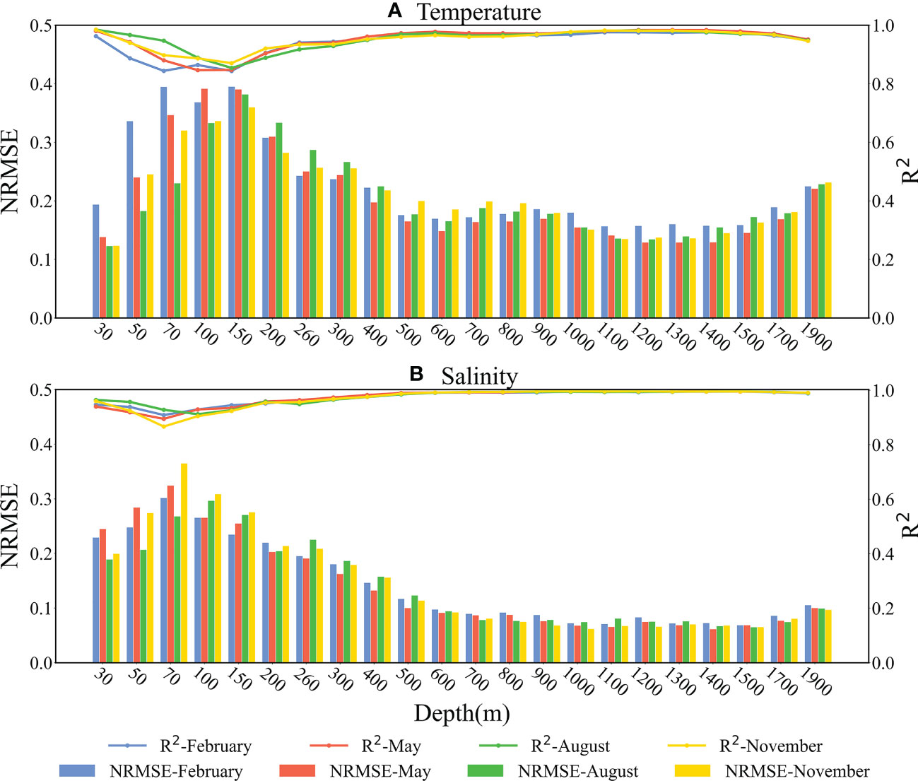
Figure 12 Seasonal performance of the CBAM-CNN model for ocean subsurface thermohaline structures estimation at different depths in the tropical Indian Ocean in 2020. Blue indicates February (winter), red indicates May (spring), green indicates August (summer), yellow indicates November(autumn), the histograms display the NRMSE, and the lines display R². (A) for temperature, (B) for salinity.

The seasonal performance of the CBAM-CNN model varies, as seen from the NRMSE and R² values for OSTS and OSSS estimation in different seasons. The vertical average NRMSE (R²) values for OSTS estimation are 0.2259 (0.9428), 0.2064 (0.9507), 0.2071 (0.9522), and 0.2110 (0.9510) for February, May, August, and November, respectively. The highest NRMSE is observed in February, and the lowest NRMSE in May, which may be attributed to changes in the monsoonal circulation system. During the winter months, the northeast monsoon winds in the tropical Indian Ocean can lead to strong upwelling of deeper layers of the ocean, which can result in large temperature variations and pose a challenge for accurate temperature estimation by the CBAM-CNN model. Conversely, during the spring months, ocean temperature tends to be more stable, with less variability, facilitating easier temperature estimation. For OSSS estimation, the vertical average NRMSE (R²) values are 0.1427 (0.9741), 0.1406 (0.9733), 0.1396 (0.9748), and 0.1451 (0.9706) for February, May, August, and November, respectively. These results suggest that the CBAM-CNN model performs better in estimating OSSS during the spring and summer seasons. In summary, the CBAM-CNN model exhibits high accuracy in estimating OSTS and OSSS for different seasons, demonstrating its robustness for the tropical Indian Ocean.

To evaluate the impact of sea surface parameters on the performance of the CBAM-CNN model, we calculate the Pearson correlation coefficients between SST, SSS, SSHA, ESSW, and NSSW with OSTS and OSSS at different depths (50 m, 100 m, 500 m, and 1000 m). By calculating the absolute value of the Pearson’s correlation coefficients, we can compare the magnitude of the correlation coefficients. Our results, presented in Figure 13, the influence of sea surface variables on temperature and salinity estimates decreases as depth increases. This suggests that sea surface variables play a more significant role in the upper ocean, especially in the shallow layers. The results show that the SST and SSHA are the two most significant factors for estimating OSTS (Figure 13A), with correlation coefficients of 0.58 and 0.44, respectively, at 50 m depth. Conversely, SSS, NSSW, and ESSW exhibit relatively weak correlations with OSTS, with most coefficients less than 0.21. In the case of OSSS estimation, SSS and SSHA are the two most influential factors (Figure 13B). Other parameters, such as SST, ESSW, and NSSW although less strongly correlated, should not be neglected, as they also affect estimation of the OSSS. Their exact role in estimation of OSTS and OSSS requires further investigation. Analyses show that the sea surface variables selected by us are effective variables for estimating the OSTS and OSSS.

FIGURE 13

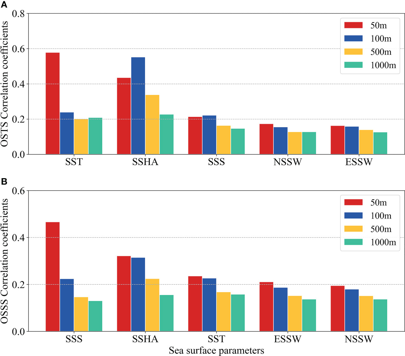
Figure 13 Correlation coefficients between the sea surface parameters (SST, SSS, SSHA, NSSW, and ESSW) and the Argo-observed (A) OSTS and (B) OSSS at 50 m (red), 100 m (blue), 500 m (golden), and 1000 m (green) from January 2010 to December 2020.

4 Summary and discussion

Accurately estimating ocean subsurface thermohaline structures is critical to understanding ocean dynamics and climate change. In this study, we propose a neural network model based on CBAM-CNN to estimate both OSTS and OSSS in the tropical Indian Ocean using sea surface data. The CBAM-CNN model integrates the attention mechanism in CNN architecture, enhancing its ability to capture spatial attention and represent complex oceanographic processes. We compare the performance of the CBAM-CNN model with the original CNN model for estimating OSTS and OSSS in the tropical Indian Ocean. The results demonstrate that the CBAM-CNN model outperforms the original CNN model, as evidenced by smaller RMSE and larger R² values. The CBAM-CNN model accurately estimates the OSTS and OSSS at different depths, with overall high accuracy across the tropical Indian Ocean. This superior performance can be attributed to the CBAM-CNN model’s enhanced ability to capture spatial attention and represent complex oceanographic processes. The study also evaluates the performance of the CBAM-CNN model from multiple perspectives, including spatial distributions, vertical profiles, and seasonal variations.

We also compare the estimated OSTS and OSSS with Argo-derived data at different depths, and the results show that the CBAM-CNN model performs well and effectively reconstructs most observed OSTS and OSSS features. Most of the observed OSTS and OSSS features can be effectively reconstructed using sea surface data via the CBAM-CNN model. Furthermore, we compare the CBAM-CNN estimated temperature and salinity profiles with the Argo profiles in four representative regions. The results demonstrate that the CBAM-CNN model accurately captures the prominent features of temperature and salinity in the tropical Indian Ocean. However, the accuracy of OSTS and OSSS estimation decreases at depths of approximately 100-150 m due to the presence of a thermocline layer, which makes accurate estimation challenging. Nonetheless, the CBAM-CNN model performs well overall and could accurately estimate OSTS and OSSS at depths below 500 m. Additionally, we evaluate the impact of sea surface parameters on the performance of the CBAM-CNN model, showing that sea surface variables play a more significant role in the upper ocean, especially in the shallow layers. SST and SSHA are the two most significant factors for estimating OSTS, whereas SSS and SSHA are the two most influential factors for OSSS estimation. Our results show that the CBAM-CNN model performs well across all four seasons, indicating that the model has a good seasonal applicability for OSTS and OSSS estimation in the tropical Indian Ocean.

In conclusion, the proposed CBAM-CNN model exhibits superior performance compared to the CNN model for estimating OSTS and OSSS in the tropical Indian Ocean. The model demonstrates high accuracy in estimating OSTS and OSSS at different depths and during different seasons. The findings of this study have implications for the understanding of oceanographic processes in the tropical Indian Ocean and provide insights for further development of oceanographic models. Nevertheless, as a statistical tool, the CBAM-CNN model has limitations in estimating extreme anomaly events. In future studies, we will employ more advanced machine learning methods and incorporate oceanic dynamic mechanisms to further enhance the estimation accuracy. Furthermore, the application of this model can be extended to cover vast oceanic regions, thus enabling precise estimations of OSTS and OSSS, and facilitating practical applications such as sound propagation, MLD estimation, and ocean disaster prediction. Additionally, the model can be further utilized to estimate other critical oceanic parameters such as velocity fields and ocean density, thus presenting an extensive area for exploration in future studies.

Data availability statement

The original contributions presented in the study are included in the article/supplementary material. Further inquiries can be directed to the corresponding authors.

Author contributions

JQ and BX contributed to the conception and design of the study. JQ, BX, and GS contributed to the methodology and modelling. JQ and BX performed the dataset analyses and visualization, with contributions from DL, JC, and BY. JQ, BX, and GS prepared the manuscript draft. All authors contributed to manuscript revision, read, and approved the submitted version.

Funding

The study was supported through the National Natural Science Foundation of China (42176010), the National Key Research and Development Program of China (2022YFF0801400), the Laoshan Laboratory (LSKJ202202400), and the Natural Science Foundation of Shandong Province, China (ZR2021MD022).

Acknowledgments

The SST data was obtained from http://apdrc.soest.hawaii.edu/dods/public_data/NOAA_SST/OISST. The SSS data was obtained from https://www.catds.fr/Products. The SSHA data was obtained from https://www.aviso.altimetry.fr/en/data/products. The SSW data was obtained from the https://www.remss.com/measurements/ccmp/. The Argo gridded data product was obtained from https://argo.ucsd.edu/data/argo-data-products/.

Conflict of interest

The authors declare that the research was conducted in the absence of any commercial or financial relationships that could be construed as a potential conflict of interest.

Publisher’s note

All claims expressed in this article are solely those of the authors and do not necessarily represent those of their affiliated organizations, or those of the publisher, the editors and the reviewers. Any product that may be evaluated in this article, or claim that may be made by its manufacturer, is not guaranteed or endorsed by the publisher.

References

Ali M., Swain D., Weller R. (2004). Estimation of ocean subsurface thermal structure from surface parameters: a neural network approach. Geophysical Res. Lett. 31 (20). doi: 10.1029/2004GL021192

CrossRef Full Text | Google Scholar

Ateweberhan M., McClanahan T. R. (2010). Relationship between historical sea-surface temperature variability and climate change-induced coral mortality in the western Indian ocean. Mar. pollut. Bull. 60 (7), 964–970. doi: 10.1016/j.marpolbul.2010.03.033

PubMed Abstract | CrossRef Full Text | Google Scholar

Atlas R., Hoffman R. N., Ardizzone J., Leidner S. M., Jusem J. C., Smith D. K., et al. (2011). A cross-calibrated, multiplatform ocean surface wind velocity product for meteorological and oceanographic applications. Bull. Am. Meteorological Soc. 92 (2), 157–174. doi: 10.1175/2010BAMS2946.1

CrossRef Full Text | Google Scholar

Bao S., Zhang R., Wang H., Yan H., Yu Y., Chen J. (2019). Salinity profile estimation in the pacific ocean from satellite surface salinity observations. J. Atmospheric Oceanic Technol. 36 (1), 53–68. doi: 10.1175/JTECH-D-17-0226.1

CrossRef Full Text | Google Scholar

Bolton T., Zanna L. (2019). Applications of deep learning to ocean data inference and subgrid parameterization. J. Adv. Modeling Earth Syst. 11 (1), 376–399. doi: 10.1029/2018MS001472

CrossRef Full Text | Google Scholar

Boutin J., Vergely J.-L., Marchand S., d’Amico F., Hasson A., Kolodziejczyk N., et al. (2018). New SMOS Sea surface salinity with reduced systematic errors and improved variability. Remote Sens. Environ. 214, 115–134. doi: 10.1016/j.rse.2018.05.022

CrossRef Full Text | Google Scholar

Cai W., Yang K., Wu L., Huang G., Santoso A., Ng B., et al. (2021). Opposite response of strong and moderate positive Indian ocean dipole to global warming. Nat. Climate Change 11 (1), 27–32. doi: 10.1038/s41558-020-00943-1

CrossRef Full Text | Google Scholar

Chu P. C., Fan C., Liu W. T. (2000). Determination of vertical thermal structure from sea surface temperature. J. Atmospheric Oceanic Technol. 17 (7), 971–979. doi: 10.1175/1520-0426(2000)017<0971:DOVTSF>2.0.CO;2

CrossRef Full Text | Google Scholar

Clevert D.-A., Unterthiner T., Hochreiter S. (2015). Fast and accurate deep network learning by exponential linear units (elus). arXiv preprint arXiv:1511.07289. doi: 10.48550/arXiv.1511.07289

CrossRef Full Text | Google Scholar

DeWitt P. (1987). Model decomposition of the monthly gulf steam/Kuroshio temperature fields. NOO Tech. Rep. 298.

Google Scholar

Fiedler P. C. (1988). Surface manifestations of subsurface thermal structure in the California current. J. Geophysical Research: Oceans 93 (C5), 4975–4983. doi: 10.1029/JC093iC05p04975

CrossRef Full Text | Google Scholar

Guinehut S., Dhomps A.-L., Larnicol G., Le Traon P.-Y. (2012). High resolution 3-d temperature and salinity fields derived from in situ and satellite observations. Ocean Sci. 8 (5), 845–857. doi: 10.5194/os-8-845-2012

CrossRef Full Text | Google Scholar

Hall N. D., Stuntz B. B., Abrams R. H. (2008). Climate change and freshwater resources. Natural Resour. Environ. 22 (3), 30–35.

Google Scholar

Ham Y.-G., Kim J.-H., Luo J.-J. (2019). Deep learning for multi-year ENSO forecasts. Nature 573 (7775), 568–572. doi: 10.5281/zenodo.3244463

PubMed Abstract | CrossRef Full Text | Google Scholar

Hauser D., Tourain C., Hermozo L., Alraddawi D., Aouf L., Chapron B., et al. (2020). New observations from the SWIM radar on-board CFOSAT: instrument validation and ocean wave measurement assessment. IEEE Trans. Geosci. Remote Sens. 59 (1), 5–26. doi: 10.1109/TGRS.2020.2994372

CrossRef Full Text | Google Scholar

Johnson G. C., Lyman J. M. (2020). Warming trends increasingly dominate global ocean. Nat. Climate Change 10 (8), 757–761. doi: 10.1038/s41558-020-0822-0

CrossRef Full Text | Google Scholar

Khedouri E., Szczechowski C., Cheney R. (1983). “Potential oceanographic applications of satellite altimetry for inferring subsurface thermal structure,” in Proceedings OCEANS’83 (San Francisco, CA, USA: IEEE), 274–280. doi: 10.1109/OCEANS.1983.1152138

CrossRef Full Text | Google Scholar

Klemas V., Yan X.-H. (2014). Subsurface and deeper ocean remote sensing from satellites: an overview and new results. Prog. oceanography 122, 1–9. doi: 10.1016/j.pocean.2013.11.010

CrossRef Full Text | Google Scholar

Levitus S., Antonov J. I., Wang J., Delworth T. L., Dixon K. W., Broccoli A. J. (2001). Anthropogenic warming of earth’s climate system. Science 292 (5515), 267–270. doi: 10.1126/science.1058154

PubMed Abstract | CrossRef Full Text | Google Scholar

Li X., Zhou Y., Wang F. (2022). Advanced information mining from ocean remote sensing imagery with deep learning. J. Remote Sensing. doi: 10.34133/2022/9849645

CrossRef Full Text | Google Scholar

Liu Y., Zhang R., Yin Y., Niu T. (2005). The application of ARGO data to the global ocean data assimilation operational system of NCC. Acta METEOROLOGICA SINICA-ENGLISH EDITION- 19 (3), 355.

Google Scholar

Luo J.-J., Sasaki W., Masumoto Y. (2012). Indian Ocean warming modulates pacific climate change. Proc. Natl. Acad. Sci. 109 (46), 18701–18706. doi: 10.1073/pnas.1210239109

CrossRef Full Text | Google Scholar

Maes C., Behringer D. (2000). Using satellite-derived sea level and temperature profiles for determining the salinity variability: a new approach. J. Geophysical Research: Oceans 105 (C4), 8537–8547. doi: 10.1029/1999JC900279

CrossRef Full Text | Google Scholar

Meijers A., Bindoff N., Rintoul S. (2011). Estimating the four-dimensional structure of the southern ocean using satellite altimetry. J. Atmospheric Oceanic Technol. 28 (4), 548–568. doi: 10.1175/2010JTECHO790.1

CrossRef Full Text | Google Scholar

Meng L., Yan C., Zhuang W., Zhang W., Geng X., Yan X.-H. (2021). Reconstructing high-resolution ocean subsurface and interior temperature and salinity anomalies from satellite observations. IEEE Trans. Geosci. Remote Sens. 60, 1–14. doi: 10.1109/TGRS.2021.3109979

CrossRef Full Text | Google Scholar

Pauthenet E., Bachelot L., Balem K., Maze G., Tréguier A. M., Roquet F., et al (2022). Four-dimensional temperature, salinity and mixed-layer depth in the Gulf Stream, reconstructed from remote-sensing and in situ observations with neural networks. Ocean Sci. 18 (4), 1221–1244. doi: 10.5194/os-18-1221-2022

CrossRef Full Text | Google Scholar

Qi J., Liu C., Chi J., Li D., Gao L., Yin B. (2022). An ensemble-based machine learning model for estimation of subsurface thermal structure in the south China Sea. Remote Sens. 14 (13), 3207. doi: 10.3390/rs14133207

CrossRef Full Text | Google Scholar

Rahaman H., Ravichandran M., Sengupta D., Harrison M. J., Griffies S. M. (2014). Development of a regional model for the north Indian ocean. Ocean Model. 75, 1–19. doi: 10.1016/j.ocemod.2013.12.005

CrossRef Full Text | Google Scholar

Rao R., Sivakumar R. (2003). Seasonal variability of sea surface salinity and salt budget of the mixed layer of the north Indian ocean. J. Geophysical Research: Oceans 108 (C1), 9–1-9-14. doi: 10.1029/2001JC000907

CrossRef Full Text | Google Scholar

Reichstein M., Camps-Valls G., Stevens B., Jung M., Denzler J., Carvalhais N. (2019). Deep learning and process understanding for data-driven earth system science. Nature 566 (7743), 195–204. doi: 10.1038/s41586-019-0912-1

PubMed Abstract | CrossRef Full Text | Google Scholar

Reynolds R. W., Rayner N. A., Smith T. M., Stokes D. C., Wang W. (2002). An improved in situ and satellite SST analysis for climate. J. Climate 15 (13), 1609–1625. doi: 10.1175/1520-0442(2002)015<1609:AIISAS>2.0.CO;2

CrossRef Full Text | Google Scholar

Roemmich D., Gilson J. (2009). The 2004–2008 mean and annual cycle of temperature, salinity, and steric height in the global ocean from the argo program. Prog. oceanography 82 (2), 81–100. doi: 10.1016/j.pocean.2009.03.004

CrossRef Full Text | Google Scholar

Schott F. A., Xie S. P., McCreary J. J. P. (2009). Indian Ocean circulation and climate variability. Rev. Geophysics 47 (1). doi: 10.1029/2007RG000245

CrossRef Full Text | Google Scholar

Smith K. Jr., Ruhl H., Bett B., Billett D., Lampitt R., Kaufmann R. (2009). Climate, carbon cycling, and deep-ocean ecosystems. Proc. Natl. Acad. Sci. 106 (46), 19211–19218. doi: 10.1073/pnas.0908322106

CrossRef Full Text | Google Scholar

Sprintall J., Gordon A. L., Koch-Larrouy A., Lee T., Potemra J. T., Pujiana K., et al. (2014). The Indonesian seas and their role in the coupled ocean–climate system. Nat. Geosci. 7 (7), 487–492. doi: 10.1038/ngeo2188

CrossRef Full Text | Google Scholar

Su H., Huang L., Li W., Yang X., Yan X. H. (2018a). Retrieving ocean subsurface temperature using a satellite-based geographically weighted regression model. J. Geophysical Research: Oceans 123 (8), 5180–5193. doi: 10.1029/2018JC014246

CrossRef Full Text | Google Scholar

Su H., Li W., Yan X. H. (2018b). Retrieving temperature anomaly in the global subsurface and deeper ocean from satellite observations. J. Geophysical Research: Oceans 123 (1), 399–410. doi: 10.1002/2017JC013631

CrossRef Full Text | Google Scholar

Su H., Wang A., Zhang T., Qin T., Du X., Yan X.-H. (2021). Super-resolution of subsurface temperature field from remote sensing observations based on machine learning. Int. J. Appl. Earth Observation Geoinformation 102, 102440. doi: 10.1016/j.jag.2021.102440

CrossRef Full Text | Google Scholar

Su H., Wu X., Yan X.-H., Kidwell A. (2015). Estimation of subsurface temperature anomaly in the Indian ocean during recent global surface warming hiatus from satellite measurements: a support vector machine approach. Remote Sens. Environ. 160, 63–71. doi: 10.1016/j.rse.2015.01.001

CrossRef Full Text | Google Scholar

Trenberth K. E., Caron J. M. (2001). Estimates of meridional atmosphere and ocean heat transports. J. Climate 14 (16), 3433–3443. doi: 10.1175/1520-0442(2001)014<3433:EOMAAO>2.0.CO;2

CrossRef Full Text | Google Scholar

Watson A. J., Schuster U., Shutler J. D., Holding T., Ashton I. G., Landschützer P., et al. (2020). Revised estimates of ocean-atmosphere CO2 flux are consistent with ocean carbon inventory. Nat. Commun. 11 (1), 4422. doi: 10.1038/s41467-020-18203-3

PubMed Abstract | CrossRef Full Text | Google Scholar

Watts D. R., Sun C., Rintoul S. (2001). A two-dimensional gravest empirical mode determined from hydrographic observations in the subantarctic front. J. Phys. Oceanography 31 (8), 2186–2209. doi: 10.1175/1520-0485(2001)031<2186:ATDGEM>2.0.CO;2

CrossRef Full Text | Google Scholar

Woo S., Park J., Lee J.-Y., Kweon I. S. (2018). “Cbam: convolutional block attention module,” in Proceedings of the European conference on computer vision (ECCV), (Munich, Germany: Springer), 3–19.

Google Scholar

Wu X., Yan X.-H., Jo Y.-H., Liu W. T. (2012). Estimation of subsurface temperature anomaly in the north Atlantic using a self-organizing map neural network. J. Atmospheric Oceanic Technol. 29 (11), 1675–1688. doi: 10.1175/JTECH-D-12-00013.1

CrossRef Full Text | Google Scholar

Xie H., Xu Q., Cheng Y., Yin X., Jia Y. (2022). Reconstruction of subsurface temperature field in the south China Sea from satellite observations based on an attention U-net model. IEEE Trans. Geosci. Remote Sens. 60, 1–19. doi: 10.1109/TGRS.2022.3200545

CrossRef Full Text | Google Scholar

Yan H., Wang H., Zhang R., Chen J., Bao S., Wang G. (2020). A dynamical-statistical approach to retrieve the ocean interior structure from surface data: SQG-mEOF-R. J. Geophysical Research: Oceans 125 (2), e2019JC015840. doi: 10.1029/2019JC015840

CrossRef Full Text | Google Scholar

Yan C., Zhu J., Xie J. (2015). An ocean data assimilation system in the Indian ocean and west pacific ocean. Adv. Atmospheric Sci. 32, 1460–1472. doi: 10.1007/s00376-015-4121-z

CrossRef Full Text | Google Scholar

Zheng G., Li X., Zhang R. H., Liu B. (2020). Purely satellite data–driven deep learning forecast of complicated tropical instability waves. Sci. Adv. 6 (29), eaba1482. doi: 10.1126/sciadv.aba1482

PubMed Abstract | CrossRef Full Text | Google Scholar