An advanced towed CTD chain for physical-biological high resolution in situ upper ocean measurements

Submesoscale eddies, fronts, and filaments are ubiquitous in the upper ocean and play an important role in biogeochemical and mixing processes as well as in the energy budget. To capture the high spatial variability of submesoscale processes, it is desirable to simultaneously resolve the vertical and horizontal gradients of hydrographic properties on scales of 10 m to 10 km. We present a revised towed CTD chain, for rapid quasi-synoptic in situ measurements of submesoscale oceanographic features, that is lighter, more robust and scientifically more useful than previous towed CTD chains. This new instrument provides a horizontal resolution of $\mathcal{O}$(1 m) and can be towed at speeds of up to 5 ms^-1 for measurements of the upper 100 m of the water column while providing a reasonable vertical resolution of $\mathcal{O}$(1 m – 10 m). Individual CTD probes are equipped with temperature, conductivity, pressure and either rapid response dissolved oxygen or fluorescence sensors at multiple depths, enabling both hydrographic and biogeochemical studies at high resolution. A flexible probe hardware allows either real-time data collection or internal data logging for offline post-processing. Finally, we outline the necessary post-processing steps and provide data examples. With the presented data examples we show and conclude that the advanced towed CTD chain is a flexible and lightweight take on the towed CTD chain concept. It can easily be adapted to scientific needs and provides high quality very high resolution oceanographic data.

1 Introduction

Submesoscale processes such as eddies, fronts and filaments play an important role in the transport of energy and nutrients, as well as for primary production, both in the coastal and open ocean (Mahadevan, 2016; McWilliams, 2016; Calil et al., 2021; Chrysagi et al., 2021). However, resolving submesoscale phenomena in situ remains challenging (Lévy et al., 2012; Lévy et al., 2018). Here, we present first results using a revised towed Conductivity-Temperature-Depth Instrument (CTD) chain that provides both, physical and biological in situ data in real-time. It allows significant flexibility with respect to the use of different research vessels, vertical resolution and sensor choice compared to previous towed CTD chains (Richardson and Hubbard, 1959; Mobley et al., 1976; Sellschopp, 1997; Adams et al., 2017).

The targeted highly dynamic features with scales between $\mathcal{O}$(1 m) to $\mathcal{O}$(10 km) are ubiquitous in the upper 100 m of the water column (McWilliams and Molemaker, 2011; Adams et al., 2017). For almost three decades, increased scientific effort has been undertaken to highlight and understand their importance, e.g. (Spall, 1995; Mahadevan and Tandon, 2006; Capet et al., 2008; Thomas et al., 2008; Lévy et al., 2012; Mahadevan, 2016; Lévy et al., 2018). Intense surface density gradients are usually associated with large vertical velocities, that may affect the air-sea as well as mixed-layer and thermocline property exchange of gases, nutrients, phytoplankton, and pollutants (Baschek, 2002; Baschek et al., 2006; Baschek and Jenkins, 2009; Osiński et al., 2010; Mahadevan, 2016).

Submesoscale processes are usually characterized by $\mathcal{O}$(1) Rossby and Richardson numbers (Thomas et al., 2008), meaning that these are regions where non-linear processes play as important a role as the Earth’s rotation and that horizontal buoyancy gradients may be as important as stratification, thus potentially inducing mixing. Despite an abundance of model-focused studies on submesoscale dynamics (Spall, 1995; Capet et al., 2008; Fox-Kemper and Ferrari, 2008; Lévy et al., 2012; Mahadevan, 2016; Calil et al., 2021), there remains an observational gap for hydrographic and especially biogeochemical in situ data, resolving energetic coupled physical-biological processes down to $\mathcal{O}$(10 m) scale (Lévy et al., 2012; Lévy et al., 2018). Consequently, there is an urgent need for improved upper ocean in situ sampling methods and instruments, not only for the observational quantification of these processes, but also to validate and parameterize model predictions (Lévy et al., 2012; McWilliams, 2016). Our towed instrument chain aims to fill the observational gap on horizontal scales between $\mathcal{O}$(1 m) to $\mathcal{O}$(10 km).

While sampling various hydrographic and biogeochemical parameters close to the surface is generally possible with relatively high resolution using pumped vessel-mounted underway systems at the submesoscale range, e.g. Lips et al. (2006); Rudnick and Klinke (2007); Petersen et al. (2018), it is more difficult to extend those measurements down to the mixed layer depth and beyond. Similarly, surface currents may be detected at high spatial and temporal resolution with radar (Lund et al., 2018), horizontal currents and acoustic backscatter over depth using established instruments such as Acoustic Doppler Current Profilers (ADCP) (Rowe and Young, 1979) or echo sounders, e.g. (Farmer et al., 1995; Farmer and Armi, 1999; Tedford et al., 2009; Velasco et al., 2018). Extending hydrographic and biogeochemical data sampling to depth – and thus complementing acoustic and underway surface measurements – requires the in situ presence of instruments, either placed at multiple depths simultaneously or tow-yoed while steaming. Examples for such complementary setups with towed instrument chains are Sellschopp et al. (2002) and Körtzinger et al. (2020).

A variety of ship towed equipment has been developed to sample submesoscale features. These can be roughly clustered in three categories. As a first group, there are tow-yoing or undulating instruments collecting data in a sawtooth pattern such as the SeaSOAR (Pollard, 1986; Ferrari and Rudnick, 2000; Pidcock et al., 2010), the Triaxus (D’Asaro et al., 2011) or the Scanfish (Brown et al., 1997; Baschek et al., 2017). The second group of instruments repeatedly collects vertical profiles while the vessel is steaming at speed, such as the underway CTD (uCTD) (Rudnick and Klinke, 2007), the Moving Vessel Profiler (Furlong et al., 1997), or the ecoCTD (Dever et al., 2020). Technically, the Expendable Bathythermograph (XBT) is also part of this group, but we do not consider it here, because it is neither reusable nor does it offer a full CTD data set. In the third group are towed thermistor and CTD chains, with multiple sensors at different depths that are towed by the vessel and allow high-resolution in situ data acquisition. Studies cited above confirm that all instruments have sampled submesoscale features such as eddies and fronts in several areas of the world ocean. In addition to the ship towed instruments we focus on, other instruments and platforms, such as autonomous underwater vehicles have also been used to sample submesoscale features, e.g. Salm et al. (2023); Carpenter et al. (2020). Despite the large set of established instruments available, providing a sampling resolution that is comparable to modelled high-resolution hydrographic and biogeochemical data sets remains challenging (Lévy et al., 2012; McWilliams, 2016).

Ship-towed undulating devices such as SeaSoar (Pollard, 1986; Pidcock et al., 2010), Triaxus (D’Asaro et al., 2011; Floeter et al., 2017) have limited horizontal resolution, given by operating depth, climb rates, ship speed and potentially sensor sampling rate. They usually require heavy ship-board equipment and therefore full-size research vessels. Instruments such as the underway CTD (Rudnick and Klinke, 2007) or the ecoCTD (Dever et al., 2020) are more lightweight than the aforementioned systems, but are limited in horizontal resolution by their drop- and recovery-rate for each cast, as well as vessel speed. Both groups of instruments are limited in their spatial resolution because they rely on a single sampling CTD instrument. Previous available instrument chains enabled data collection at several depths simultaneously, but were limited in sensor choice (Richardson and Hubbard, 1959; Mobley et al., 1976) and required heavy machinery to be deployed and recovered (Sellschopp, 1997; Sellschopp et al., 2006; Andrew et al., 2010).

These shortcomings of available instruments and the need to resolve horizontal features on the $\mathcal{O}$(10 m) have driven our efforts to develop an advanced towed CTD chain. Our goal is to provide a flexible, robust, lightweight and easy-to-use towed CTD chain for studies in areas where strong submesoscale dynamics create large spatial variability, such as ocean fronts and eddies, or in coastal upwelling regions and estuaries where fine-scale processes are relevant. We took the established concept of a towed CTD chain like in Sellschopp (1997), combined it with the developments towards a lightweight stand-alone CTD chain by Baschek (personal communication, 2018) and developed it further towards the current state of technology. Compared to existing towed CTD chains with multiple stand-alone probes, our towed chain is flexible in terms of number of attached CTD probes, see Figure 1 for a system overview. In addition, probes may be equipped with – among others – fast oxygen and fluorescence sensors to study the fine-scale patchiness of phytoplankton blooms in situ (Omta et al., 2008; Mahadevan, 2016; Lévy et al., 2018). Because our towed instrument chain offers standard CTD sensors plus one additional sensor we call the sensor packages CTD+ probes. The system is an array of individual CTD instruments, hence we refer to our towed CTD chain as the Towed Instrument Array, hereafter called TIA. Using standalone CTD+ probes provides two possible modes of TIA operation. The TIA can either sample and display data in real-time using a deck-unit (Real-Time Mode, RTM), thus being very useful in scenarios requiring adaptive sampling strategies, or it is used in a much simpler and lighter memory logging version (Memory Mode, MM). Both versions do not require a large vessel for deployment or underway measurements and are simple to set up and operate.

FIGURE 1

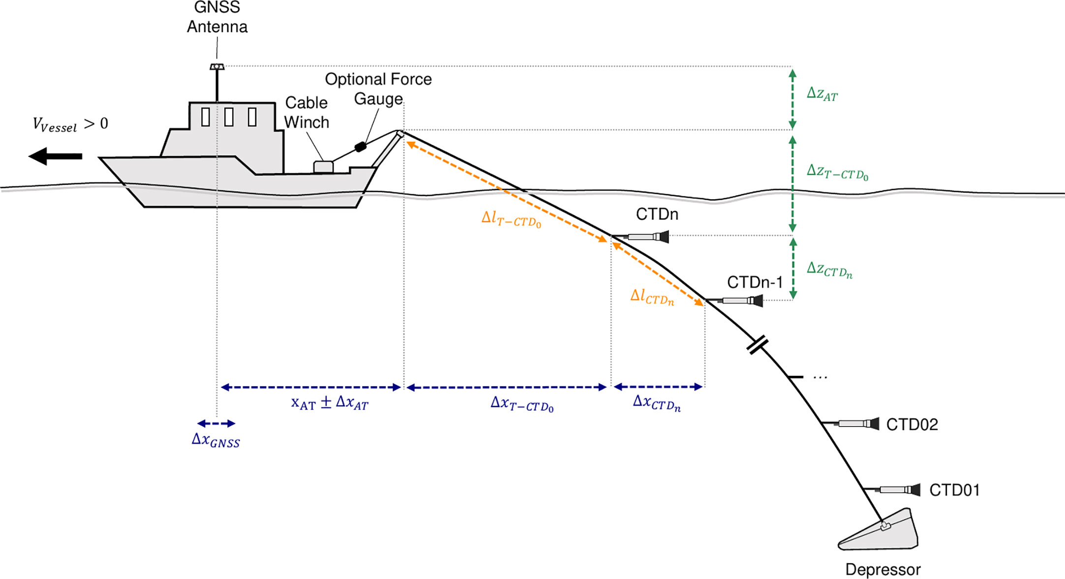
Figure 1 Schematic of the TIA system and its components in a typical configuration. Required distances for data processing are added for reference.

2 Materials and methods

2.1 TIA technology

2.1.1 TIA CTD+ probes

The TIA uses a modified version of Sea & Sun Technologies CTD48mc¹ standard CTD probe assembly. One CTD48mc unit holds all necessary power, sampling and communication electronics inside a cylindrical titanium housing of 48 mm diameter and about 450 mm length (Figure 2A). All probes are equipped with a Sea & Sun Technology GmbH PT100 sensor for temperature, a Sea & Sun Technology GmbH OEM 7-pole conductivity cell (Ginzkey, 1977)² and an OEM pressure sensor (Keller 7LD PA)³ . The fourth sensor slot can be equipped with one additional sensor for oxygen, turbidity, pH, redox (OPR), or fluorometers. Table 1 lists the sensors’ properties.

FIGURE 2

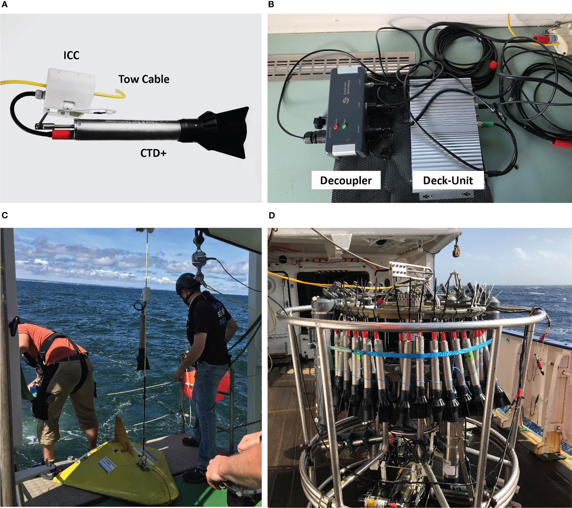
Figure 2 The main components of a TIA. (A) CTD+ probe equipped with an inductive coupling clamp (ICC) mounted to the tow cable. (B) Set up of Deck-Unit and Decoupler for real-time communication with TIA’s CTD+ probes. (C) RTM TIA right before deployment on RV Ludwig Prandtl, one CTD+ probe is mounted right above the V-Fin depressor to provide real-time readings of approximate depressor depth. (D) A typical set up for cross calibrating TIA CTD+ probes against an external CTD on RV Meteor. Photograph in panel (A) courtesy of Sea & Sun Technology GmbH, panels (B-D) are own work.

TABLE 1

Table 1 Sensor data sheet values for standard TIA sensors.

In addition to the sensors, each CTD+ probe is equipped with an accurate Real Time Clock (RTC) and three standard 18650 rechargeable Lithium-Ion batteries resulting in a nominal capacity of about 12 Wh. The battery capacity allows for safe planning of more than 24 h continuous sampling at maximum sampling rate. Longer deployments of more than 36 h have been recorded successfully. Between deployments, the batteries are recharged using the TIA charging stations (see section 2.1.5) without opening the pressure tubes. An internal charge controller supervises the charging process and protects the batteries from potentially harmful operating conditions.

The CTD+ probes achieve a maximum sampling rate of about 7 Hz, depending on sensor configuration. This translates to a nominal horizontal resolution as small as 0.36 m at a typical cruise speed of 5 kn for individual readings. For practical data use, some averaging might be necessary to improve data reliability, effectively limiting horizontal resolution to be $\mathcal{O}$(1 m).

All CTD+ probes are equipped with a communications modem for the optional transfer of sampled data via the inductive coupling clamps – see section 2.1.3 – and the tow cable to the topside decoupler for real time data evaluation by the operator. The modem equipment may be switched off for MM deployments to save power. Independent from operating mode, collected data is continuously stored on internal permanent storage for later download and evaluation. A wet-mateable 8 pin connector at the connector endcap of each probe facilitates data download and battery charging. Because individual probes provide their own internal battery, memory, and all necessary sampling logic, operation of the TIA is resistant to single hardware failure.

2.1.2 Tow cable and depressor

In contrast to previous tow chains, contemporary materials allow the use of very thin cables with considerable breaking strengths while still having a well isolated copper core inside for data transmission in RTM. A typical TIA cable has a diameter of about 7 mm and consists of a copper core, electric insulation, inner polyurethane coating, Aramid fibre braid, and an outer polyurethane coating (see the yellow cable in Figure 2A). If used in MM only, the TIA can be operated with an even thinner rope such as Dyneema^® SK78 12 strand rope with 4 to 6 mm diameter.

To counter the drag forces acting on the tow rope or cable, a V-fin type depressor is used at the lower end of the tow cable. The weight and size of the depressor is determined by the desired depth, cable type, cable length and boat type. Generally, a larger depressor reaches deeper. In addition, if the depressor is large enough, it may carry one of the CTD+ probes and – in RTM – provide information of current maximum depth of the TIA via the deck-unit. A force gauge maybe installed to monitor acting forces on the TIA in real-time, see section 2.2 for further details and data examples.

2.1.3 Optional inductive data transmission

Many of the concepts used for the optional inductive data transmission in RTM-TIA deployments are described in Sellschopp (1997) and are developed further to let RTM-TIA benefit from technological advances and allow for greater flexibility in terms of setup and sensor placement.

Flexible placement of CTD+ probes along the tow cable is achieved by Sea & Sun Technology GmbH’s self-tightening clamp. The clamp integrates a ferrite core for inductive data transmission on the cable. Hence, the clamps are called Inductive Coupling Clamp (ICC). For the clamp to work, it is crucial to maintain the ability to open the ferrite core while mounting the clamp to the cable. Figures 2A, C show a CTD+ equipped with an ICC and mounted to the tow cable, in Figure 2B the use of an ICC as interface between decoupler and tow cable is partially shown in the upper right. While the ICC is a key component in RTM-TIA deployments, it is not necessary to use it in MM deployments. Instead, low-cost lockable carabiners and rope slings may be used.

Data transmission is realized in a multipeer network architecture consisting of several CTD+ probes and the topside interface, the deck-unit. The deck-unit manages the data traffic in this network. CTD+ probes collect data continuously and send data blocks at programmable intervals. Using a timed and blocked data transmission scheme keeps the networking overhead small and avoids packet collision.

The CTD+ probes sample at a maximum of about 7 Hz and save all samples internally for later download in both operating modes. Real-time data transmission is, however, limited to a 1 Hz subset for TIAs with 15 CTD+ probes due to bandwidth limitations. Yet, this subset offers enough resolution to observe submesoscale features in real-time during data collection providing insight into the water column to quickly adapt vessel course for tracking submesoscale features. Tweaking the data transmission payload and transmission intervals facilitates adding more probes to RTM-TIAs. For MM configurations, there is no theoretical limit of probes, except for excessive drag. It is also possible to add additional memory CTD+ probes to RTM-TIA configurations to enhance vertical resolution in post-processing.

Since the tow cable only has a single copper conductor, the electric loop has to be closed through the seawater. A small bare metal electrode (A_s ≈ 60 cm²) connected to the lower end of the copper conductor next to the depressor is sufficient. The top electrode may also be a small bare metal part towed through the water or, on steel-hull vessels, the hull of the towing vessel can be used. Either way, the topside electrode must be connected to the top end of the tow cable passing the data signal decoupling electronics, that consist of a modified ICC and another modem. Figure 2B shows the deck-unit and decoupling equipment.

2.1.4 Optional deck-unit and data visualisation

A deck-unit completes the set of instrumentation of a RTM-TIA system (Figure 2B). The deck-unit serves as the interface between the TIA operator and CTD+ probes. It enables real-time communication and setup of the individual probes via the tow cable while RTM-TIA is deployed. Communication via the tow cable is limited to the transfer of collected data subsets and – for simplicity – a very limited set of commands for the CTD+ probes. Next, the deck-unit is used as an interface to connect required ancillary inputs to the TIA system such as Global Navigation Satellite System (GNSS) receivers. Finally, the computer in the deck-unit processes the incoming data and runs a webserver providing real-time data visualisation. The data visualisation of the RTM-TIA is therefore easily accessible via the vessel’s Ethernet network at any network enabled workspace. The deck-unit itself must be placed somewhere close to the tow cable and decoupler, see Figure 2B.

2.1.5 Charging stations

After deployment, the CTD+ probes need to be recharged and raw data should be downloaded from the probes’ memories. Charging many individual probes and downloading data after a deployment requires to connect each probe to a suitable charger using the wet mateable connectors. To simplify this process, Sea & Sun Technology GmbH developed charging stations for automatically charging six CTD+ probes at a time. Complete charging takes about 6 to 8 hours for fully depleted batteries. Meanwhile, the charging stations automatically download the full resolution data sets from the probes’ memories to their internal storage. The charging stations keep track of the files they have already downloaded and automatically apply a naming scheme with the unique probe ID and a timestamp to the files for easy file identification. By default, the charging stations will not erase files from the internal probe memory, thus creating an additional copy of the raw data.

The charging stations are accessible via Ethernet and provide a web interface to supervise battery charging and data transfer. The mass storage of the charging stations may be mounted as a samba network share on any client PC, making further data transfer a simple and efficient task. All actions applied to the collected data sets hereafter are considered as post-processing and will be described in the section 2.3.3 below.

2.1.6 Time synchronisation

The TIA uses stand-alone CTD+ probes with integrated RTCs. Therefore, a reliable and accurate time synchronisation between all probes prior to deployment is mandatory. To have the same time synchronisation process for both operating modes, RTM and MM, the charging stations are set up to synchronise all connected CTD+ probes’ RTCs with a central time source using Network Time Protocol (NTP).

The probes’ internal RTCs are stable with a typical drift of about 0.5 s d⁻¹. Setting time via the charging stations once prior to deployments is hence considered sufficient, given the overall system accuracy. See section 2.4.5.

2.1.7 Winch

A winch is not strictly necessary for deployment and recovery of a TIA, but it simplifies the process. Almost any kind of winch is feasible, for example small friction winches have been used successfully during the Tara Ocean Foundations Mission Microbiomes⁴ and the Madeira Island Wakes experiment presented below.

TIAs flexibility in terms of the winch is made possible by the strict lightweight design and the detachable CTD+ sensors. This means, that the only requirement the winch must fulfil is to have enough power to handle the forces acting on the system. Because data transmission in RTM-TIAs is done via contactless inductive coupling, there is neither the need for a slip ring on the winch, nor for an accurate cable reeling in the winche’s drum.

2.1.8 Safety considerations

Towing a cable with a depressor through the water bears the risk of hitting floating objects, fishing nets or the seafloor at speed. To prevent loss of the instrument as well as damage to the towing vessel, we use simple, low-cost weak-links of known breaking strength to connect the top end of the tow cable to the vessel. The weak-link must be placed outside the vessel to avoid potential injuries of people by cable lashing in case of a failure. On the TIA end of the weak-link, we place a pickup buoy equipped with GNSS sender and flashlight for recovery of the instrument.

The breaking strength of the weak link is adjusted to match a maximum of 0.5 times the breaking strength of the main TIA cable or, if the towing vessel is small, as low as possible to save the boat from damage. As a rule of thumb, we used 300 daN weaklinks for a 120 m TIA in coastal areas with rigid-hulled inflatable boats and 700 to 1000 daN weak-links on full size research vessels for about 500 m of cable with a breaking strength of about 2000 daN.

Care must be taken during recovery of the depressor under adverse weather conditions, as excessive kiting of the depressor is potentially dangerous. Yet, a TIA reduces many risks inherently involved during deployment and recovery of earlier towed CTD chain instruments by avoiding the need for heavy machinery and mandatory manual guidance of fins, cables and fairings through pulleys, see the report of Andrew et al. (2010) for details.

2.2 Tow mechanics

Governed by the acting forces, an instrument chain of given length l towed through the water with v_vessel > 0 will adjust to a characteristic convex shape over depth z at force equilibrium (Deschner et al., 2023). Simultaneously, a considerable horizontal distance x emerges between towing point and depressor (Figure 1). Because the TIAs flexible design allows many different configurations, the chain shape and the acting forces during a TIA operation should be reliably estimated in advance. As a tool, we apply a TIA model put forward by Deschner et al. (2023), that is based on pendulum theory using Lagrange mechanics. It simulates TIA sensor depths impinged by the dominant forces under different operation scenarios and helps to choose appropriate cable and depressor types for the desired tasks. The TIA configuration employed in the M160 cruise serves as a prominent example of the model capabilities. It had the longest cable length (480 m) to date with 21 attached CTD+ probes operated in RTM. The model computes the characteristic convex shape of the cable and agrees well with the sensor positions.

Figure 3A shows a selection of different TIA setups used with cable lengths between 125 m and 480 m and demonstrates sizeable dependencies of chain shape from sensor placement, vessel speed and depressor type. Figure 3B illustrates the rather small variation between different methods of TIA shape approximations. It is interesting to note that the positions of the CTD+ probes nicely follow the curve of a tractrix, the theoretical solution for a curve along which an object moves under the influence of friction, when pulled on a horizontal plane. The tractrix fit results are added to Figure 3B (red, dash-dot) together with chain shapes computed using Pythagoras’ theorem (gray, dashed) and output from two runs with the TIA simulation of Deschner et al. (2023). For the TIA simulation, n_k is the added number of computing nodes between the probes (n_p). All data from M160 shown in Figure 3 have been collected during relatively stable flight conditions on 13th December 2019 between 14:30 and 15:10 UTC, see the gray shaded area in Figure 4. A detailed discussion of the potential Probe Location Error for each shape approximation is given in section 2.4.3.

FIGURE 3

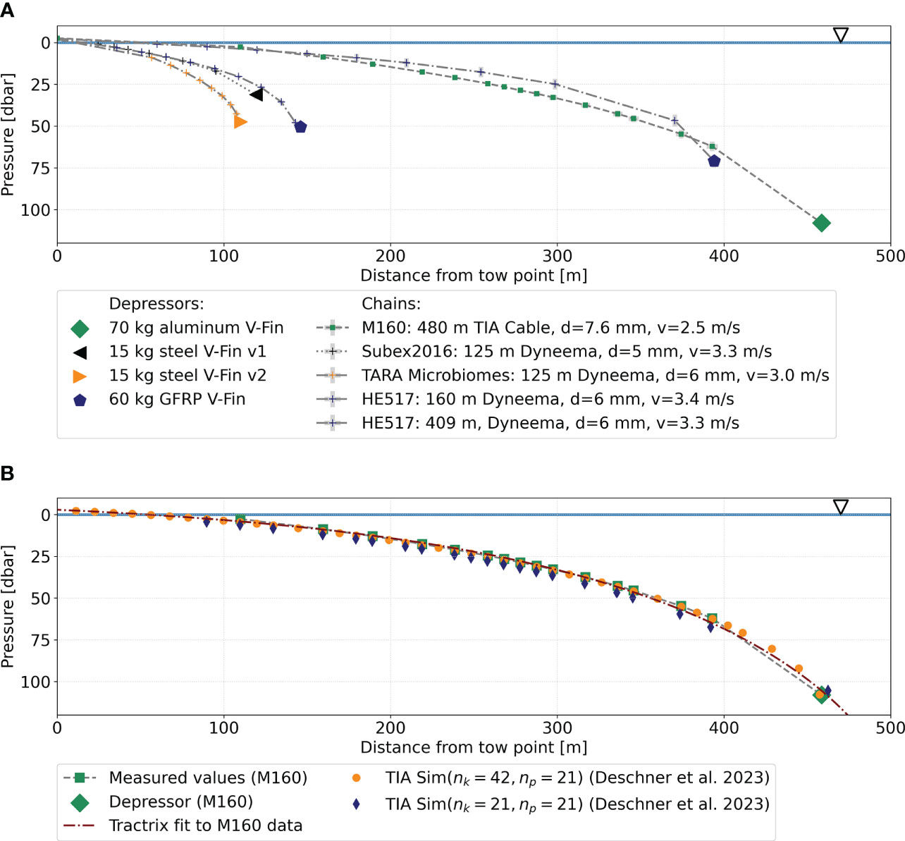
Figure 3 Panel (A) Approximations of tow chain shapes during towing at constant speed from different setups and deployments. Coloured marks along the linearly interpolated cable shape show depth averages of the individual CTD+ probes at their positions on the cable. Larger symbols indicate different depressor types. Panel (B) illustrates three different ways of approximating the real TIA shape. The aspect ratio of the plots is set to one to visualise the horizontal displacement of the TIA behind the vessel compared to reached depths.

FIGURE 4

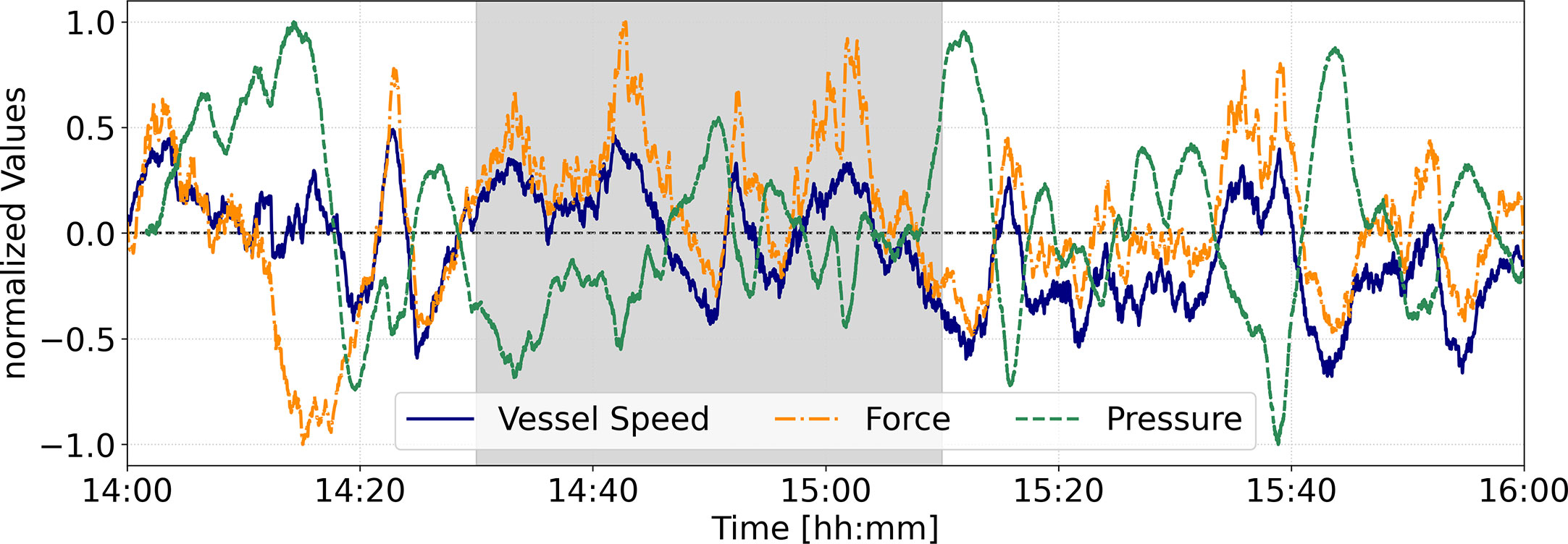
Figure 4 A section of Vessel Speed (SOG) (blue, solid), deepest CTM pressure (green, dashed) and tow point force (orange, dash-dotted) obtained during cruise M160 with a 480 m long TIA and a 70 kg V-fin depressor on a straight track. All values are normalized across the section. Pressure data is shifted by about 99 s to the right with respect to speed data to better visualize correlation. Vessel speed and force data correlate well with force shifted by 3.7 s to the left. The gray shaded area indicates the example subset used in Figure 3.

During the M160 cruise, we operated the TIA with an additional force gauge at the tow point to gain a better understanding of the induced forces acting on the TIA due to vessel motion (Figure 2C). The data example in Figure 4 has been collected on a straight track on 13th December 2019 between 14:00 and 16:00 UTC. We observed acting forces in the range of 154 to 435 daN with a mean of 313 ± 49daN, which is well below the breaking strength of the weak link at 1000 daN and the cable itself with 2000 daN, speed over ground (SOG) during the transect was 2.6 m s^-1 ± 0.4 m s^-1 while the pressure of the deepest probe was 109.4 dbar ± 5.6 dbar. Figure 4 shows normalised time series of force, pressure and SOG during the transect illustrating dependencies between vessel speed, instrument depth and acting forces.

A correlation analysis using Pearson’s product-moment correlation method revealed that the signals for force, SOG and pressure are shifted in time with respect to each other. Correlation between force and SOG is maximal for a shift of -3.7 s with a correlation coefficient of 0.64 s, while pressure and SOG correlate best at a 98.8 s shift with a correlation coefficient of -0.48. Figure 4 is already corrected for the computed time shifts to better visualize the correlation between the signals. These observations imply a relatively long settling time of the TIA after changes in vessel speed until it again reaches force equilibrium and stable depths of the probes. The observed time t_eq for reaching force equilibrium after speed changes agrees well with the computations of Deschner et al. (2023), see their section 3.4 and their Figure 16.

From our data, tows deeper than about 110 m seem not to be possible at a tow speed larger than 2.5 ms^-1 with the described setup and equipment. Future TIA setups may, however, well overcome this limitation by using stronger cables and more efficient depressors. For comparison, typical measured forces for smaller MM TIA configurations with 120 m of rope and a smaller 15 kg depressor, are in the range of 150 to 300 daN.

2.3 TIA data acquisition

2.3.1 Preparations

The TIA is an arrangement of several independent instruments sampling autonomously. Nevertheless, a TIA data set is supposed to represent a quasi-2-d vertical section of the water column comprised of n individual horizontal profiles. Consequently, individual CTD+ probes must be aligned well in time and space. The sensors must be both calibrated against a known standard and among each other in order to provide comparable readings and a reliable quasi-2-d information, refer to section 2.4.4 for numbers and details. Collecting high quality raw data with TIA therefore requires careful pre-deployment preparations

By design, TIA allows complete flexibility to place CTD+ probes along the cable. At the same time, having the accurate probe’s locations along the cable is crucial for posterior data geo-referencing and data interpretation. Placing the probes at the best location, needs a priori knowledge about target area, sampling depths, survey speed, number n of probes and the length of the TIA. The CTD+ probe depths z or p correspond to distances l along the cable. Following our best practice, probe locations along the cable are marked with a cumulative accuracy of ± 1 cm. Together with offsets along the vessel’s fore-aft, starboard, and vertical axis individual probe locations are later referenced to the GNSS antenna (Figure 1).

2.3.2 Collecting data

Each CTD+ sensor is calibrated at the probe manufacturer’s facilities prior to and after each cruise; each probe is delivered with a calibration protocol. During cruises, a cross-calibration or intercalibration cast with all of the individual CTD+ probes before each deployment against an external reference CTD and against each other is highly recommended to achieve sufficient inter-sensor precision (section 2.4.4).

Deploying the TIA requires at least two people. The general procedure is as follows:

1. The vessel maintains a speed < 2 kn to avoid hitting the hull or propeller of the vessel. If conditions allow, stopping the vessel might be an option.

2. The depressor is lowered into the water until it runs stable. If one probe is mounted directly to the depressor in RTM, the communication can now be tested using the deck-unit.

3. The TIA cable is lowered step by step and all probes are mounted to the cable/rope according to the prepared marks on the cable/rope.

4. Optional for RTM TIAs: Once all probes are on the cable and in the water, the communication is checked.

5. The cable is lowered further to the desired length and the weak link and recovery buoy are mounted.

6. The vessel picks up the desired speed.

In both operating modes – RTM and MM – the CTD+ probes collect and store data internally in the same manner. In RTM, the deck-unit further offers the option to supervise the data collection in real-time. A subset of the collected data is received at regular intervals and the deck-unit merges the ocean state parameters with external GNSS data to provide various plots, see previous sections 2.1.3 and 2.1.4 for more details.

After recovering the TIA, binary raw data are downloaded from the CTD+ probes using the charging stations. The first processing step converts them into physical units using intercalibration functions and constants from the probe’s provider with text-files as output. The conversion also includes computation of dependent quantities such as practical salinity, potential density and others that use water pressure, temperature and conductivity as input. Currently, we still use the EOS-80 standard algorithms (Fofonoff and Millard, 1983) for raw data conversion and quality control routines, because when the development of the instrument and software toolboxes started in 2009, TEOS-10 (McDougall and Barker, 2011) was not yet available. The migration to full TEOS-10 support is straightforward and will be available in the next release of the raw data conversion software and TIA processing package.

At this stage TIA data text-files for each probe comprise time series with timestamps provided by the probes’ internal RTCs. For geo-referencing, one has to exploit another set of files containing logged NMEA0183 telegrams from an extra on-board GNSS receiver. The NMEA files must include at least the Recommended Minimum Navigation Information (RMC). Alternatively, using the NMEA telegrams GGA⁵ and ZDA⁶ in conjunction is an option. Both the TIA data text-files and corresponding NMEA files are used during post-processing.

2.3.3 Data processing

In the previous sections, we described the TIA as a system consisting of a number of individual CTD+ probes. However, our main intention is to allow quasi-2-d interpretations of TIA data. Consequently, post-processing of TIA data sets is split into two major task packages each consisting of several subtasks. Figure 5 provides an illustration of this workflow:

1. CTD processing package: Quality checks of the collected data for each probe independently.

2. TIA processing package: Internal consistency check of the TIA data set regarding RTC timestamps, horizontal positioning, ocean state data; geo-referencing of the TIA data set; creating output files for quasi-2-d ocean state analyses.

FIGURE 5

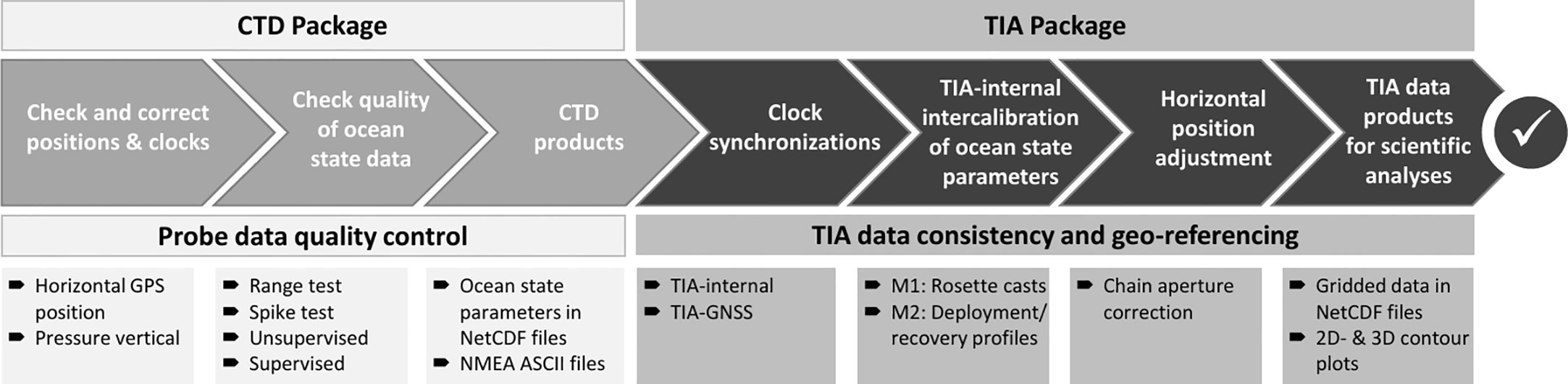
Figure 5 Flow chart of the post-processing steps applied to TIA data sets before scientific usage.

In the CTD processing package, all CTD data have to pass filters:

● for each time, a reliable horizontal position fix must exist

● for each time, a reliable proxy for the vertical position, i.e. pressure, must exist

● a range test (plausibility test) with user defined lower and upper limits

● an outlier removal procedure with user defined window sizes, for both data values and time

Data that do not pass a filter, are flagged according to the rules of the SeaDataNet Quality Control Standards used in the COSYNA observing system (Baschek et al., 2017; SeaDataNet, 2017), ranging from good over bad to not existent. Data regarded as bad or not existent are not considered in subsequent filters or data processing. The quality flags of the directly measured parameters are also transferred to the dependent variables derived from them. After the filters are applied automatically, the results are visually inspected. Flags can be undone, accepted or added. Visual inspection is of foremost importance for parameters that detect particle densities, namely Chl-A fluorescence, as these exhibit significant natural fluctuations towards high extremes. This double checking also helps to detect and flag unrecoverable human errors such as not removing protective caps on sensors.

As output of the CTD processing package, meta data, data, quality flags and documentations of applied flags are stored in netCDF-files comprising global and variable attributes. To meet the FAIR principles (Wilkinson et al., 2016) the output data format obeys the netCDF Climate and Forecast (CF) Metadata Conventions⁷ adopted by Hereon in the Binding Regulations for Storing Data as netCDF Files⁸.

The TIA processing package merges the individual TIA CTD+ ocean state data and the GNSS files into a comprehensive set of files jointly gridded along UTC timestamps. This package includes essential tasks to achieve data consistencies within the TIA data set, that fulfill the specified accuracies and precisions in timing, geo-location and sensor calibration. Refer to section 2.4 for details. The TIA processing package allows to skip these tasks or to generate data sets with or without further corrections.

2.3.3.1 Clock synchronisation

To achieve consistent $\mathcal{O}$(1m) horizontal positioning between all CTD+ probes within the TIA, their RTCs have to run synchronously within $\mathcal{O}$(1s) for typical towing speeds of 2.5 ms^-1. This requirement is essential for the subsequent post-processing steps and therefore checked in the first place. Corrections for offsets and drift, require at least two synchronised timestamps common to all CTD+ probes. Exact synchronisation of the CTD+ RTCs is essential for subsequent post-processing tasks. Hence, the first step of the TIA processing package is to check whether the on-board clock synchronisation has achieved $\mathcal{O}$(1s) precision. This and further corrections for offsets and drift, require at least two synchronised time stamps common to all CTD+ probes probes, assuming constant clock drifts over time. If these timestamps are only provided by the internal RTCs of the CTD+ probes, a second step for synchronising the CTD+ clocks with GNSS time is performed.

2.3.3.2 TIA internal intercalibration of ocean state parameters

The filters applied in the CTD processing package cannot detect or correct any data inconsistencies between the individual CTD+ probes. Depending on available intercalibration casts, at least one of two distinct intercalibration methods is applied. In section 2.4.4, we describe the two methods in detail and outline the effects and limitations of intercalibration. Intercalibration provides intercalibration tables with correction values for each directly measured parameter and CTD+ probe. The derived ocean state variables are re-computed using the intercalibration tables.

2.3.3.3 Horizontal TIA shape correction

In section 2.2 we described the characteristic shape of the TIA imposing considerable, horizontal distances Δx between vessel and CTD+ probes, compare sketch in Figure 1. The horizontal distances for each probe depend on the placement along the cable Δl of each probe. To transform the series of horizontal profiles of each CTD+ into consistent vertical profiles, the probes’ distances in relation to a horizontal reference point, e.g. the GNSS location of the vessel, are compensated through an alignment of each data series in time. We call this step Horizontal TIA Shape Correction (HTSC). The corresponding time lags of the data records are computed by the fraction of the horizontal distances of the CTD+ probes $\text{Δ}{x}_{AT}+\text{Δ}{x}_{T-CT{D}_0}+{\displaystyle \sum _{i=0}^{i=n}\text{Δ}{x}_{CT{D}_i}}$ over the ship speed v_vessel(t). Using HTSC assumes a non-changing water column over the time period of the largest occurring time lag, refer to section 2.4.3 for more details and numbers. The HTSC is carried out at each timestamp independently to reflect TIA’s dynamic flight conditions as good as possible.

2.3.3.4 Output products

For subsequent analyses, the data of all probes are interpolated to a joint time grid with the timestamps of the slowest data collection rate. The quality flags are set accordingly. Then all probe data is geo-referenced using HTSC. Finally, the gridded and geo-referenced data are stored in a new set of netCDF files for subsequent scientific analyses. They contain data values, their quality flags, and meta data such as the clock synchronisation, intercalibration parameters and HTSC correction data. This allows to reverse previous TIA processing package processing steps, if needed. The files have the joint, horizontally TIA shape corrected time grid as abscissa and the depths as ordinate. However, no interpolation and gridding with respect to the water depth is done: the creation of 2-dimensional data arrays is regarded as part of the subsequent scientific analysis. For this reason, all data examples shown in section 4 are scatter plots of the TIA data set.

A full TIA data set stores all data, i.e. the binary raw data, converted CTD+ text-data files and two sets of netCDF-files with meta data. The first being the output of the CTD processing package, the second of the TIA processing package. All post-processing steps are thus documented. Please note that in contrast to the CTD processing package, the TIA processing package processing steps change data values beyond the quality flagging.

Processing a day of TIA data requires about half a day of post-processing work including file preparations and documentations files.

2.4 Error considerations

In the following, the main sources of errors and uncertainties of the TIA are estimated. Take note, that for TIA it is difficult to completely distinguish between errors and uncertainties as they are intertwined. Hence, we refer to their product as errors. The list is not complete as error sources and magnitudes depend much on the particular setup. As an example, we refer to data collected during the M160 cruise as this was the most complex TIA setup to date.

2.4.1 Time

Synchronising all CTD+ clocks within $\mathcal{O}$(1 s) is the most crucial part in TIA data collection, in order to resolve the shape and the location of submesoscale features. As mentioned in section 2.1.6, TIAs probes are equipped with RTCs to provide accurate timing with a typical drift of less than 0.5 s d^-1. Synchronisation is done using a GNSS timeserver via Network Time Protocol directly before and after each deployment. The remaining uncertainty of probe RTC timing is ideally only determined by the Network Time Protocol time sync jitter that is $\mathcal{O}$(10 ms). Compared to the sampling times of $\mathcal{O}$(100 ms) or the crossing of individual submesoscale features, timing is considered to be accurate. For typical cruise speeds of about 2.5 m s^-1, the absolute maximum combined timing errors theoretically translate to horizontal errors of less than 0.2 m after drift corrections.

Compared to the requirements for correctly measuring of the gradients at the edges of the submesoscale features, the P, T and C sensors have response times that are a factor of 10 lower than the required $\mathcal{O}$(1 s), as listed in in Table 1. For Chl-A, vendor provided response times are < 1 s for the Turner Cyclops-7F sensor and < 0.6 s for the Turner C-Fluor sensor. The < 2 s response time for the O₂-sensor seem to be just at the limit to reliably record the sharp edges of submesoscale features. However, visual inspection of strong O₂-gradients did not reveal noticeable differences in the timing of temperature and O₂-patterns.

2.4.2 Depth

Each CTD+ probe is equipped with pressure, temperature, and conductivity sensors. Depth (z) is computed from those using the EOS-80 equations, see Fofonoff and Millard (1983), their section 4, pages 25ff. for details. The concrete implementation uses the function seawater.eos80.dpth from python package seawater⁹. Its overall accuracy depends on the pressure reading as well as the density profile above the sampling location. The density profile of the water column above is in turn derived from the salinity measured with sensors located above on the chain. The pressure sensors of the CTD+ probes have a measurement range of 0 to 200 dbar with a typical accuracy of <0.15 % FS, translating into an error of typically <0.3 dbar. The error magnitude in z introduced by reconstructing the density profiles from the limited number of CTD+ probes in the vertical must be estimated case by case. Due to the horizontal distances between the CTD+ probes imposed by TIAs shape, a density profile can only be correctly reconstructed after all CTD+ probes have passed a certain location and under the assumption of a non-changing water column during that time, see next section 2.4.3 for numbers and details. The number of interpolation points is limited by the number of CTD+ probes used and separated by depths on the order of $\mathcal{O}$(1–10 m). For the M160 cruise, estimation of differences in depth between equating water pressure in dbar with depth in m calculated from the EOS-80 pressure to depth conversion yielded an absolute error less than 0.5 m down to 110 m sampling depth. In this case, a linear interpolation between the measurements may reproduce the real profiles quite well as computed from the example transect shown in in Figure 6. This might be different in the presence of strong pycnoclines and emphasizes the need for case by case investigation.

FIGURE 6

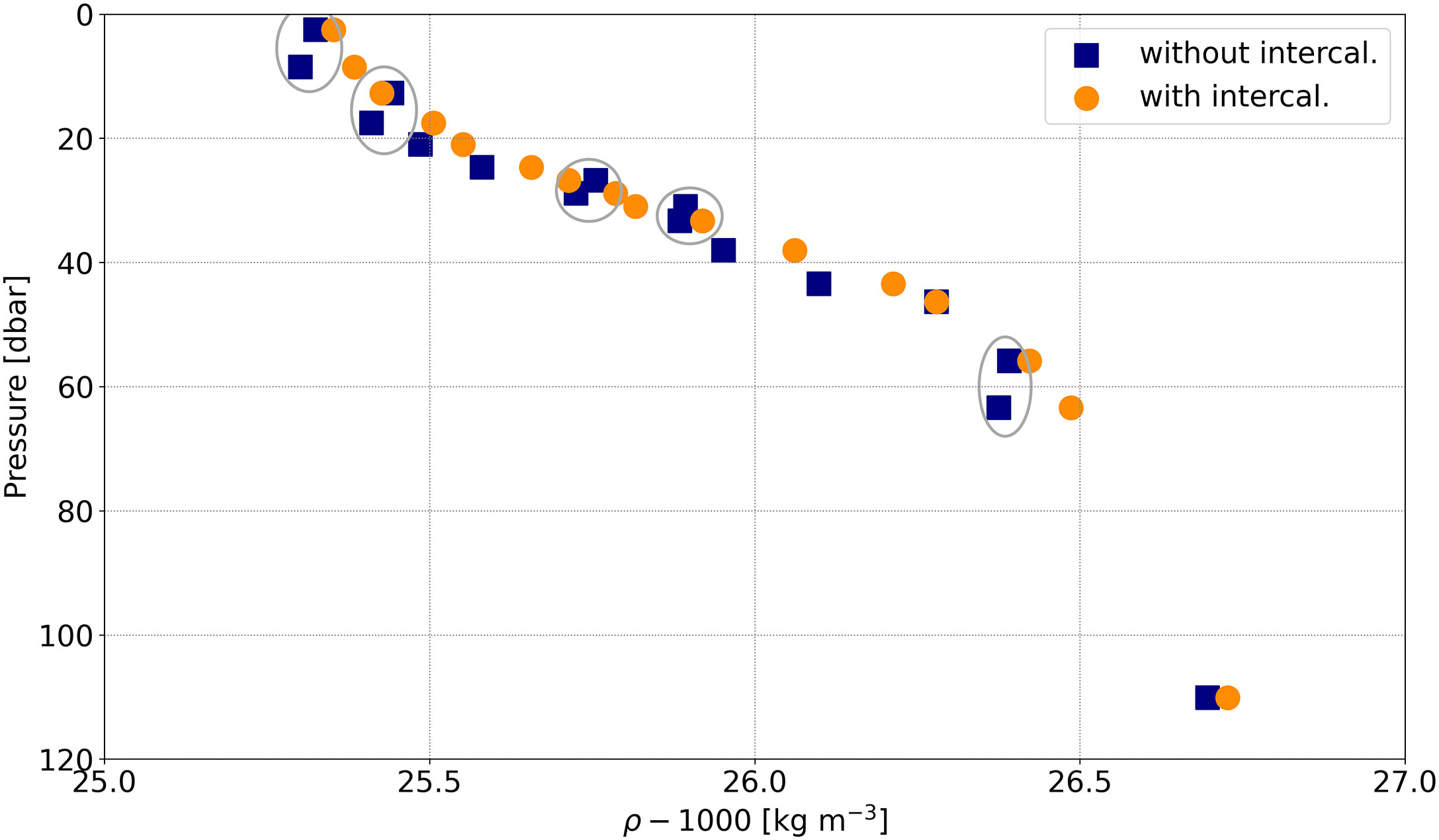
Figure 6 Potential density profile, computed as an average over a 9 km part of a transect collected on December 13, 2019 southwest of the Cape Verde island Fogo. Blue squares represent the data before, orange dots after intercalibration. Gray ellipses indicate cases before intercalibration where water densities seem to be locally increased.

2.4.3 Geo-reference

The accuracy of geo-referencing of TIA data depends on numerous factors. Figure 1 shows the involved auxiliary instruments and the offsets necessary to compute a geo-location for each sample. There are two types of errors: The first one affects the average position of the whole TIA in space, the second the position of the CTD+ probes relative to each other.

A GNSS receiver is used as the base for geo-referencing. GNSS inherent errors are of the first type and depend on its operation mode. In coastal areas or with stable internet connection, it is possible to receive GNSS correction signals from a Beacon, a known base station (RTK-fixed) or via network (Networked Transport of RTCM via Internet Protocol, NTRIP). Without the correction signals, the accuracy deteriorates from ± 1 cm to GNSS stand-alone accuracy of ± 5 – 10 m (Kaplan and Hegarty, 2006). The errors introduced by the GNSS system in use influence all TIA data the same way. Since the GNSS error is considered to be random, its effect may be mitigated by averaging or filtering.

In addition, the distance between GNSS antenna and tow point must be measured. Its components are Δx_AT and Δz_AT. A possible cross-ship component Δy of this distance is neglected. The result is usually accurate to few cm and may be neglected as it affects all TIA probes in the same way. All GNSS related errors also depend on vessel motion as the GNSS antenna may move differently in space than the tow point. We do, however, not consider those errors.

The second type of errors involves the different horizontal positions of the CTD+ probes along the cable relative to a joint reference position, dictated by the characteristic shape of the TIA. For quantification, the distances l along the tow cable between tow point and each CTD+ probe and their depths are needed, $\text{Δ}{l}_{T-CT{D}_0}$ and $\text{Δ}{l}_{CT{D}_n}$ in Figure 1.

In our TIA survey configurations, the sum of all horizontal distances between the uppermost and the deepest probe of the TIA chain ranges from 20 m for our shortest to more than 350 m for our longest chain, see Figures 1, 3. Thus, at a typical survey speed of 2.5 ms^-1, the timestamp at a fixed specific horizontal position may differ by 8 – 140 s.

Manually measuring all distances l along the TIA cable sequentially, i.e. as an incremental measure, increases the uncertainty in l with each added probe. Given, that we measure each interval in l with an accuracy of ± 1 mm, we estimate the sum of the incremental errors to be on order of ± 1 cm at the utmost probe location l_n. The measurements for l do not take potential cable stretching into account.

In our processing workflow, we compute the horizontal distances of the CTD+ probes to the position of the GNSS antenna under the assumptions of (1) neglecting the stretching of the cable as typical stretching values for Aramid or Kevlar fibres are < 1% (Sanborn et al., 2015), and (2) approximating the shape of the cable between two neighboured CTD+ probes as a straight line. This uses Pythagoras’ theorem with the measured values for pressure (p) or depth (z) and probe distance along the cable (l), leading to a minor overestimation of the horizontal distances δ_x, see Figure 7. Both assumptions introduce a Probe Location Error (PLE) ${\delta }_l=\sqrt{{\delta }_x^2+{\delta }_y^2}$, with the error δ_y along depth. Values with δ_x < 0 are shifted towards the vessel and δ_y < 0 towards larger depths.

To quantify the PLE, we analyze the smallest distances δ_l according to Deschner et al. (2023) and a tractrix fit related to (2). The TIA simulation has been computed twice: A high-resolution run with n_k = 42 m, n_p = 21 and a lower resolution run with n_k = n_p = 21. n_p is the number of simulated probes, n_k is the number of nodes dividing the straight lines between the probes into smaller subsections. The resolution n_k = 42 is chosen according to solutions, where the positions of each probe converge to the real shape of the TIA. The drag- and depressor forces acting on the TIA (case n_k = 42) are varied until the measured maximum depth of ∼108 m is reached. The same variables are used for both simulations. Additionally, a tractrix is fitted to the measured M160 data points and δ_l is computed for both.

The orange dashed line in Figure 7 outlines the accuracy of the model results concerning the M160 data. The greatest PLE is less than 2 m for the first two CTD+ probes where all following CTD+ probes are closer than 1 m to the M160 data. In comparison, the fitted tractrix (red, dash-dotted) deviates strongest for the first two CTD+ probes (squares) and the PLE decreases with distance. The subfigure in Figure 7 reveals, that the modeled results (orange squares) deviate more in the vertical and the fitted data (red squares) more in the horizontal. The M160 data are fixed in depth and assumption (2) hence leads to a PLE in the horizontal. The simulation computes the positions in equilibrium with regard to the applied forces. Therefore, the deviations correspond to both directions but are astonishingly small. The starred line in Figure 7 shows the PLEs between the two model runs.

FIGURE 7

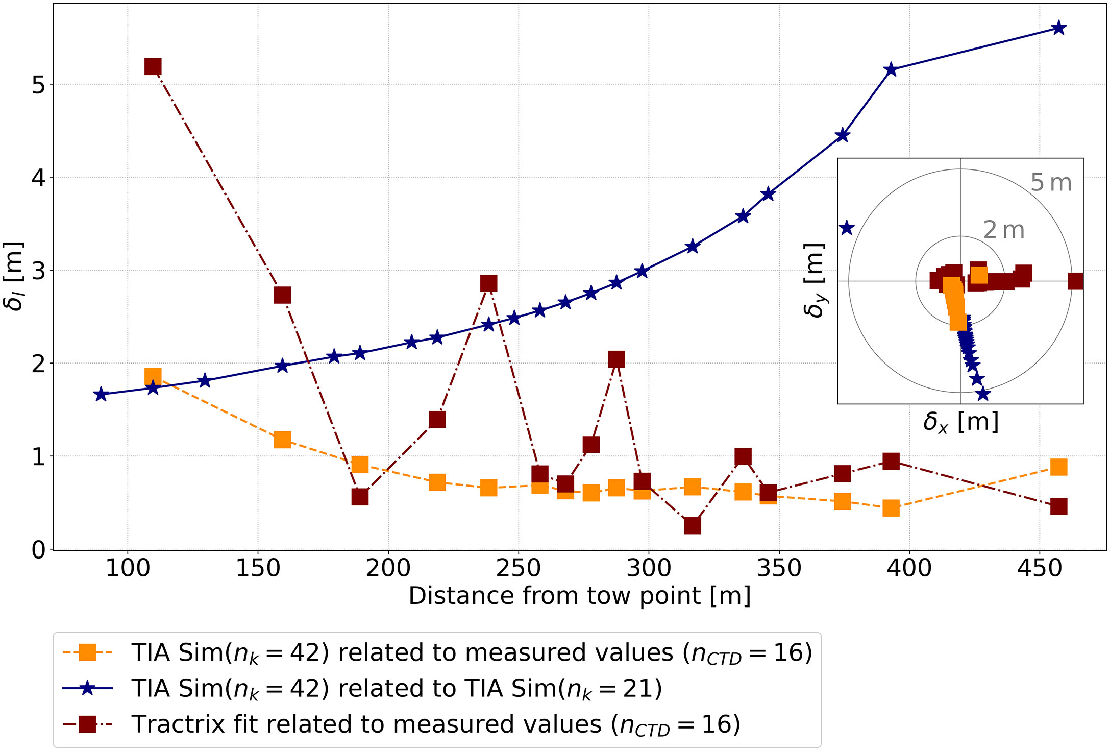
Figure 7 The dashed line shows the norm of the PLE of the high-resolution model results compared to the M160 configuration to be <2 m. The PLE between the tractrix fit and the M160 configuration is <5.5 m. Hence, a theoretical PLE to estimate assumption (2) in section 4.4.3 can be computed (stars) and we find the maximum error of ∼5.5 m for the last CTD+. This is of the same order as assumed by (1) in section 2.4.3. The subplot decomposes the PLE into its Cartesian components.

If the high-resolution results were the converged real solution then assumption (2) leads to a theoretical PLE increasing with distance, with the maximum PLE δ_l ~ 5.5 m. It is of the same order as expected from assumption (1), they seem to cancel each other nearly out, and are below the proposed 10 m scale necessary to resolve the submesoscale features.

An error contribution by sideway displacement of the TIA due to cross-currents and ship yaw is unknown, but for a 480 m TIA and a displacement angle of 10° we find ∼5 m at most. Significant positioning errors occur during and after turns of the vessel. Chapman (1984) and Grosenbaugh (2007) indicated that the computation of a proper geo-location for turns is not simple to do. Using TIA data collected during and after turns is therefore not recommended. The TIA package provides tools to manually cut or flag those data.

2.4.4 Ocean state parameters

The TIA measures the parameters pressure (P), temperature (T), and conductivity (C) at all CTD+ probe positions. Oxygen saturation (O₂) as well as Chl-A are measured alternately at preselected positions along the tow chain. The inter-sensor precision of the sensors is a peculiarly sensitive issue of a TIA, as, in contrast to profiling or undulating devices, the vertical variations of the parameters are derived from numerous independently operating sensors. The accuracies of the measurements rely on the laboratory calibration coefficients of the providers, but need to be checked for each survey, as the sensor response may change with time due to sensor drift. Lab calibrations prior and after each cruise allow principally to estimate the sensor drift, under the assumption of drift being linear over time. Sensor drift correction is, however, not yet implemented into the TIA package due to time constraints and prioritization of other correction measures.

For Chl-A, one has to keep in mind that sensor calibration was done with lab samples that have a response different to phytoplankton in the ocean, which in turn depends on the existing species and on the sensor type. Please note that TIA operations usually prohibit the collection of in situ water samples for calibration.

As listed in Table 1 the vendor provided accuracies for P, T and C are near or even below 1 ‰. However, transect data collected during the M160 cruise revealed intriguing examples that further intercalibration of the TIA CTD+ T and C sensors was needed. Figure 6 displays the vertical profile of potential sea water density ρ averaged horizontally over a 9 km long part of the transect also shown and discussed in section 4.1. The averaging proves the necessity for intercalibration by revealing the systematic nature of sensor errors. The 9 km track was chosen for TIA’s stable flight conditions. The vertical profile shows gradients of about 0.035 kg m⁻³ m⁻¹. Over most parts of the TIA, the typical probe distances in depth are about 5 m, corresponding to ρ differences of 0.175 kg m⁻³ or 7 ‰. The laboratory calibration coefficients of the providers lead to seemingly increasing ρ with depth wrongly suggesting gravitationally unstable conditions at the depths around some probes, highlighted with gray ellipses at about 5, 15, 28, 32, and 60 dbar in Figure 6.

Higher degrees of TIA internal precision were achieved by two ways of ancillary in-situ sensor intercalibration. The optimal method is to collect extra vertical intercalibration cast data with all probes attached to a single frame at the same height as shown in Figure 2D. We call this Intercalibration Method 1 (M1). A similar but smaller setup might be used on smaller vessels. If other calibrated CTD systems independent of TIA are operated on the vessel, the arrangement should include a joint reference CTD on the vessel.

In case M1 is not possible, one may correlate data taken at the same depth during the deployment and recovery phase of the TIA operation instead. This is Intercalibration Method 2 (M2) and has some disadvantages. For instance, due to the changing water bodies during the deployment/recovery of TIA, which can take up to 15 min for long TIA setups. M2 works, but is not as accurate as M1.

For the M160 cruise, the required level of precision was achieved using M1 when possible and M2 in all other cases. The example in Figure 6 illustrates nicely that it is not sufficient to rely on laboratory calibration only. Having intercalibration profiles should receive adequate attention during cruise planning.

2.4.5 Summary of error sources

Data processing is mandatory for TIA data sets in order to achieve consistent and accurate data sets. The panels in Figure 8 illustrate nicely the results of the minimum required processing steps CTD+ clock synchronisation, HTSC, and intercalibration for a potential density (σ = ρ -1000 kg m^-3) data set recorded during the M160 cruise. Figure 8 shows a subset of the example transect presented in section 4.1, the same subset is used for Figure 6. All panels use the same colormap and axes.

FIGURE 8

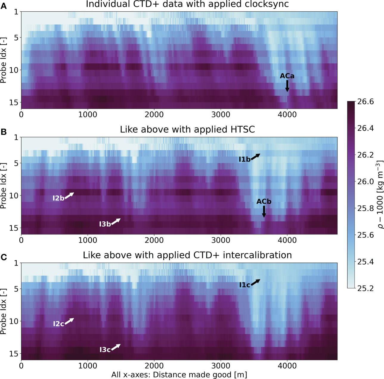
Figure 8 An illustration of data quality improvements after application of certain post-processing steps. Panel (A) shows individual raw CTD+ data with applied clock synchronisation. Panel (B) shows the same data set with additional htsc, i.e. all samples are referenced to the same geo-location, effectively providing a set of vertical profiles over distance, observe the markers labelled with AC for an illustration. Panel (C) illustrates the need for CTD+ intercalibration and the effect it has on the data set. Layers of a seemingly unstable density profile could be removed as highlighted by markers labelled with I.

Figure 8A shows the raw time series data of the individual CTD+ probes after RTC sync. (B) is data set (A) with applied HTSC. Note, that the tilted features in panel (A) are removed in panels (B) and (C), as well as the horizontal shift of roughly 350 m between markers ACa and ACb. The size of the shift is different for each probe and depends on probe position and force equilibrium. Comparison with the calculated TIA shapes in Figure 3B reveals the shift size to be reasonable. Figure 8C is data set (B) improved by intercalibration, i.e. with all corrections the TIA package provides. While in panel (B), some CTD+ data sets give the false impression of gravitationally unstable layered water columns, for instance at markers I1b, I2b, I3b, panel (C) shows the effect of proper intercalibration, identifying observations in panel (B) as artefacts (compare Figure 6). While at marker I2c an offset is still perceptible, the other two examples I1c, I3c show good agreement with the surrounding probes after intercalibration.

As a summary we provide Table 2 with an overview of the potential errors of TIA and appropriate correction measures. Table 2 lists also the orders of magnitude of required accuracy/precision to correctly resolve submesoscale features. The listed requirements result from the formulated goal to resolve horizontal features down to $\mathcal{O}$(1 m) as outlined in the introduction.

TABLE 2

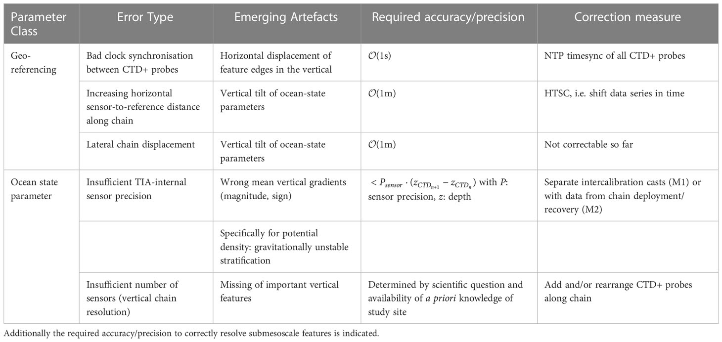
Table 2 A summary of potential error sources for TIA measurements and potential correction measures.

3 An idealized comparison of ship towed instruments for submesoscale observations

To obtain an estimation of the capabilities and limitations of the TIA in terms of sampling resolution, an idealized simulation illustrates how different types of instruments would sample a density gradient as shown in Figure 9A with operating parameters listed in Table 3. For this comparison, we take the corrected density profile shown in Figure 6, repeat it indefinitely and place an isopycnal gradient. The gradient is an idealized version of the isopycnal gradient shown in Figure 10B close to the 2 km mark, with a vertical displacement of 40 m over a distance of 500 m.

FIGURE 9

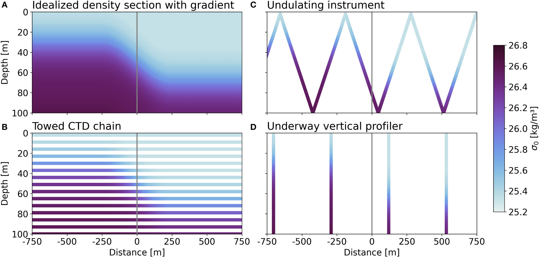
Figure 9 Illustration of sampling patterns from three different kinds of idealized ship towed instruments. Panel (A) shows an idealized density section with a gradient over depth at distance 0 m all three instruments are sampling. Panels (B-D) show the samples the different instruments would measure using the operating parameters given in Table 3. All plots are scatter plots without using any kind of interpolation. Simulation of density gradients across a sharp front obtained with different types of instruments. The centered gray line in all panels indicates where the center of the front is in the model. The constructed sampling data includes a gradient in density (A).

FIGURE 10

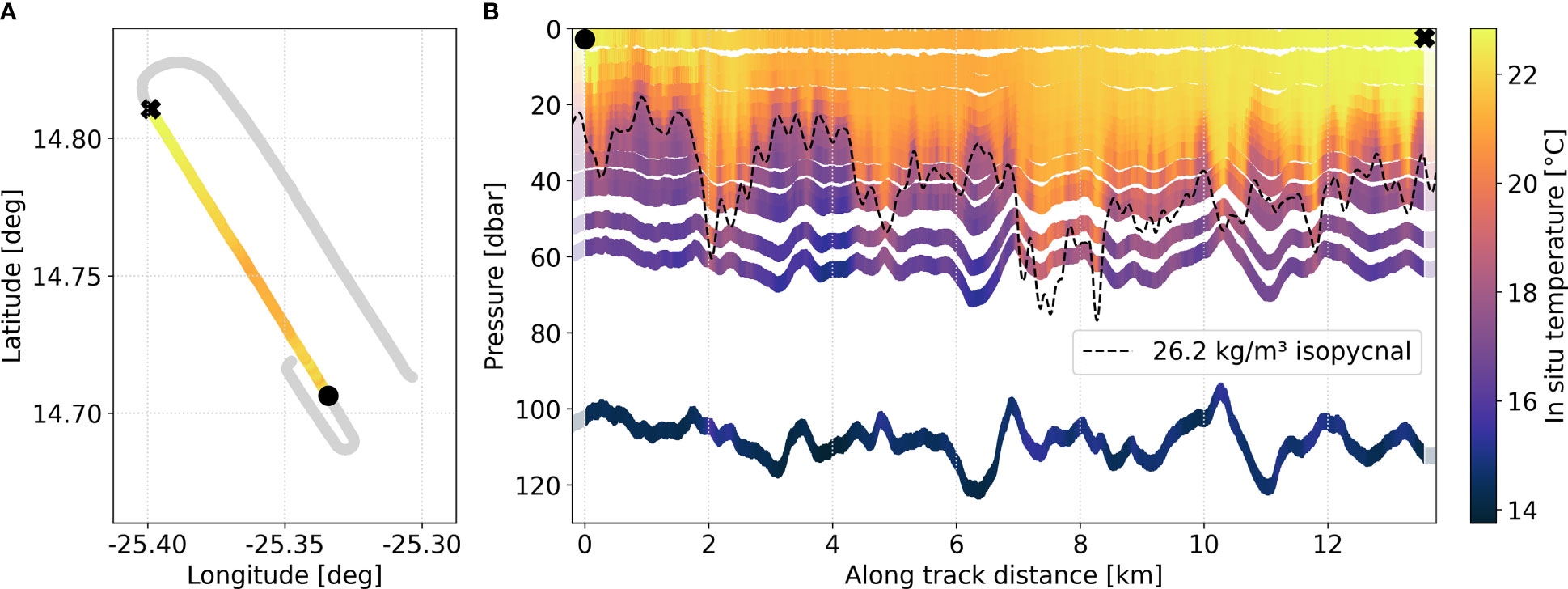
Figure 10 Example transect taken during cruise M160 on RV Meteor on December 13, 2019 south west of Cape Verde archipelago. Panel (A) shows the shiptrack of the whole TIA data set in gray with a color overlay for the topmost temperature readings. The black dot marks the beginning, the cross the end of the transect. Panel (B) shows the same transect data over depth for all probes. Both panels share the same colorbar.

As noted before, the TIA is one of several instruments used for in situ sampling of upper ocean submesoscale features that we have grouped into undulating, vertical profiling and towed chain instruments. Because the three groups have their intrinsic advantages and disadvantages, we include the undulating and vertical profiling instruments into our idealized comparison. We select one instrument from each group to simulate realistic operating parameters. We choose the SeaSOAR with operating parameters as in Pollard (1986) to represent undulating instruments. The uCTD (Rudnick and Klinke, 2007) represents the group of underway vertical profilers and our simulated TIA is set up similarly as we used it during the M160 cruise on the German research vessel Meteor (Körtzinger et al., 2020). The three instruments are towed virtually through the density field to mimic data collection according to their respective operating parameters, see Table 3 for a full list. All three instruments are set up to sample as fast as possible: The simulated uCTD does not take time for tail spooling or other handling into account, thus representing an optimised deployment in terms of horizontal spacing of the profiles. For the SeaSOAR, we increased the CTD sampling rate to more contemporary 10 Hz. Other parameters for the simulation include an assumed vessel speed of 3 m s⁻¹ and a profiling depth of 100 m for all instruments. We note that both, the SeaSOAR and the uCTD, can easily reach much greater depths than TIA. Despite this limitation given by TIAs operating depth, we consider the comparison to be valid, because both other instrument types could be used for similar upper ocean or coastal ocean studies like the presented TIA.

TABLE 3

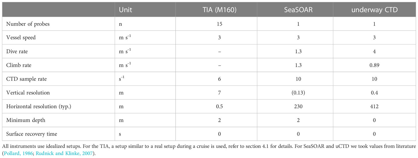
Table 3 Operating parameters for the three instruments simulated for the comparison study.

We simulate the data collection with the three virtual instruments throughout the idealized density field from left to right. The sampling patterns and individual samples are plotted in Figures 9B–D. Data collection for all instruments starts well before the plotted section, meaning that the relative locations of the undulating and vertical profiles in relation to the center of the density gradient are arbitrary. The code for the comparison scripts is available at Zenodo (Kock et al., 2023) and may be used to redo the comparison with different parameters.

Panels (B)-(D) show TIAs higher sampling density and better sample distribution across the model section when compared to the other two instrument types. While TIA lacks a vertical resolution below 1 m, it provides about 3 to 4 orders of magnitude higher horizontal resolution, see Table 3 for numbers. The results for undulating instrument and vertical profiler therefore depend much more on the horizontal location of the profile relative to the gradient. Panel (B) illustrates how TIA data sets are in fact a collection of very high resolution horizontal profiles collected at several depths simultaneously. Each of the horizontal profiles might be analysed individually enabling several isobar following studies like in Rudnick and Ferrari (1999) and Ferrari and Rudnick (2000) in one pass.

This idealized comparison shows the distinct strengths and weaknesses of the three instrument types in terms of sampling patterns. While the TIA might be the ideal instrument to resolve horizontal features across several length scales it does not provide the detailed information on vertical gradients like the other two instruments. On the other hand, undulating and underway vertical profiling instruments do not resolve the very fine-scale horizontal part of the submesoscale, i.e. less than $\mathcal{O}$(100 m). In conclusion, the choice of the correct instruments depends much on the scientific question and is beyond the scope of this article.

4 Example results

4.1 MOSES Eddy Study II - M160

This data set was collected during the MOSES¹⁰ (Weber et al., 2021) Eddy Study II cruise on German RV Meteor on December 13, 2019 southeast of Cape Verde islands Brava and Fogo (Körtzinger et al., 2020). The cruise identifier is M160. The TIA was set up in RTM with a total of 21 CTD+ probes with a non-uniform vertical spacing with enhanced vertical resolution in the first 60 m of the water column. One probe was installed directly on the V-fin depressor to obtain readings of the total depth of the 480 m long TIA. The CTD+ probes used during M160 were prototypes with firmware problems only identified during the field work, and fixed thereafter. Five of those CTD+ probes unfortunately did not record any data or data was unrecoverable. The final data set is reduced to 16 CTD+ probes.

The cruise track was determined with airborne remote sensing of the water temperature using an infrared camera mounted to a motor glider. The transect cuts through part of a mesoscale eddy forming in the lee of the islands. The aim was to measure submesoscale instabilities forming within that eddy. Infrared imagery indicated the location and extent of a submesoscale cold water filament of about 5 km width. Figure 10 shows the cruise track plotted with a superimposed color track indicating the topmost CTD+ in situ temperature readings during a 14 km long crossing of the cold filament. Crossing the whole filament revealed two very fine-scale frontal zones at km 3 and km 8, respectively. The colormap is the same for both panels.

The TIA was towed with a speed over ground of about 2.5 ms^-1 using a tow chain cable of 7.6 mm diameter and a 70 kg V-fin aluminum depressor¹¹. Variations in depth are caused by sea state and vessel speed variations. The sea state was an estimated 3 to 4 with moderate swell. The transect shown was taken roughly between 14:30 and 16:00 UTC.

With this setup, the TIA is able to resolve features with horizontal scales of $\mathcal{O}$(10 m) revealing an abundance of fine-scale vertical excursions of warm, less dense water along the transect as indicated by the 26.2 kg m⁻³ isopycnal in Figure 10B. While the depth of the isopycnal varies between 20 m and 75 m across the transect, at km 7, the horizontal density gradient reaches 0.6 kg m⁻³ over a distance of only 250 m. The strong gradients seem to be characteristic for the submesoscale dynamics within the mesoscale eddy. Furthermore, TIA reveals the presence and vertical structure of a colder and denser filament about 5 km wide, between along track km 3 and 8 in Figure 10B, confirming the findings of the motor glider in-situ. A mixed layer depth of about 30 to 80 m is characteristic for this region in December (de Boyer Montégut et al., 2004).

4.2 Mission microbiomes

The TIA was also used in many legs of the Mission Microbiomes covering many different regions of the Atlantic Ocean onboard the Schooner Tara as part of the AtlantECO project¹². Here, we briefly present an example of the data collected during the Amazon River plume experiment in order to highlight TIA’s capabilities in detecting the river plume structure. A detailed analysis of TIA data from the entire Microbiomes cruise will be part of upcoming articles after Microbiomes has finished.

On Tara, a 125 m MM version with 9 CTD+ probes, equally spaced over depth was used. Deployment and recovery was done with a small electric capstan-style winch. All CTD+ sensors used during Microbiomes had received major firmware upgrades after the M160 cruise (section 4.1) and did not have time synchronisation issues or other unpredictable problems anymore. With the upgrades, the TIA proved to be a highly reliable instrument over more than one year, with only a single CTD+ probe failing in late 2022.

Tara cruised at a speed of around 3 m s⁻¹ with the TIA reaching a stable depth of about 50 m. Sensor spacing was about 4 m between 10 and 50 m depth. On Tara, the TIA has been used heavily during transits and successfully collected data for 20 transect with single transects as long as 467 km over a time span of 40 h without problems.

Figure 11A shows a part of a transect collected with Tara in late August 2021 crossing filaments transporting fresher waters of the Amazon River plume. The TIA successfully sampled variations across scales from $\mathcal{O}$(100 km) down to $\mathcal{O}$(100 m) essentially covering both mesoscale and submesoscale in one pass. In Figure 11B we can easily identify the Amazon River plume by its lower haline water on top of more haline ocean water. We can further see the vertical and horizontal extent of the river plume filament. Close to the 50 km mark, we observe strong salinity fluctuations at a depth of about 22 m of much smaller horizontal size than the general stratification created by the river plume implying the presence of mixing processes at the interface between fresher river water and sea water. The interactions of Amazon River plume and North Brazil Current system are analysed in detail in Olivier et al. (2022).

FIGURE 11

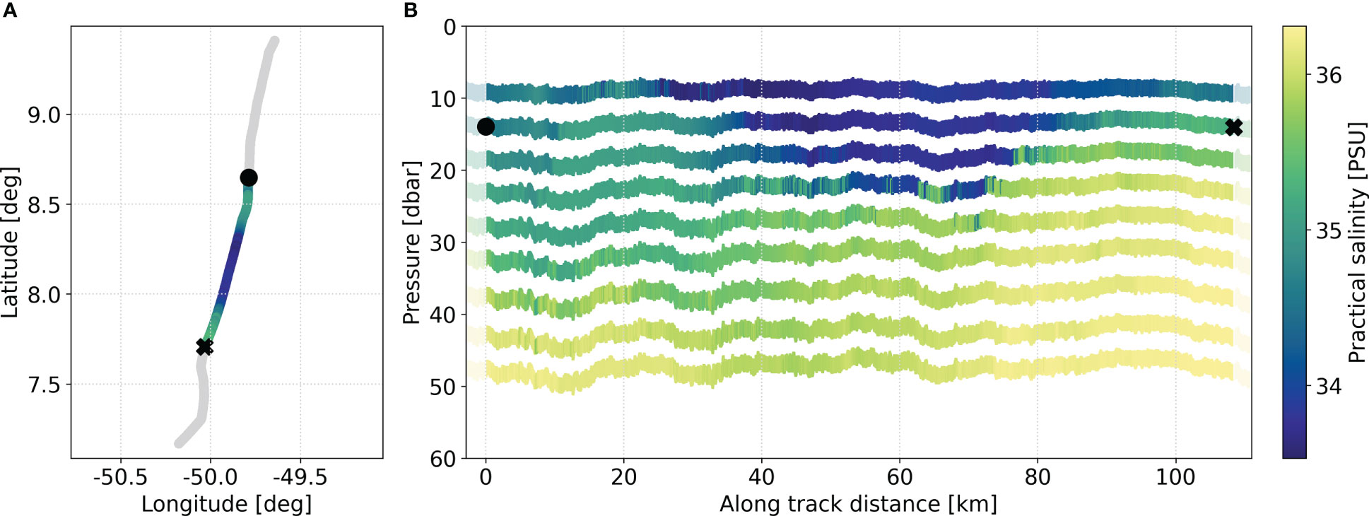
Figure 11 Example data set collected with Schooner Tara during the Mission Microbiomes of the Tara Ocean Foundation in August 2021. Panel (A) shows the shiptrack of the transect with a color overlay of practical salinity readings from the shallowest CTD+ of the TIA. The black circle and cross mark start and end of the transect subsection shown in Panel (B). Panel (B) shows the practical salinity readings for each CTD+ over distance and depth. Both panels share the same colorbar.

4.3 Madeira Island Wakes experiment

As a third example of TIAs flexibility and capabilities, we show a transect of dissolved oxygen data collected on 11th August 2022 south-west off the Portuguese island Madeira near the city of Calheta. The cruise aimed at studying the warm island wake forming during summer caused by Madeiras topology and dominant winds, e.g. Azevedo et al. (2021); Caldeira et al. (2002). During the cruise, Multi-scale Ultra-high Resolution (MUR) (JPL MUR MEaSUREs Project, 2015) satellite sea-surface temperature images showed an incoming cyclonic eddy with a cold water core potentially rich in dissolved oxygen. Because the coastal area near Calheta is used for both, traditional and aquaculture fishing, cold, oxygen enriched waters are of particular interest to local stakeholders.

A 125 m long RTM TIA was installed on the 13 m long motor yacht Dori. A total of 12 equally depth spaced CTD+ probes were used, 6 of them equipped with fast dissolved oxygen sensors, the other 6 were equipped with fluorometers providing Chl-A concentration estimates. For deployment and recovery, a Northlift LH700 hydraulic hauler winch¹³ was used together with a manually operated cable drum to store TIAs cable.

We set out with TIA to measure the water properties of the eddy from outside the rim towards the cold core. This was, however, not possible due to the small boat and increasingly adverse weather conditions combined with considerable cross-sea swells. For safety reasons, the course was changed back towards the calmer area inside the island wake. Nonetheless, TIA collected an interesting data set revealing oxygen (O₂) richer waters transported at least at the rim of the eddy. Figure 12 shows the ship track in panel (A) and the O₂ concentration data collected with TIA in panel (B). O₂ concentrations were computed from O₂ saturation readings using the TEOS-10 python gsw¹⁴ package version 3.6.16 (McDougall and Barker, 2011). The function gsw.O2_sol_SP_pt has been used to be in line the EOS-80 standard used for other TIA data in this paper. The colour of the ship track represents the oxygen readings at about 29 m depth as indicated by the red markers in panel (B). During the whole transect, the ship’s speed over ground was about 1.7 m s⁻¹.

FIGURE 12

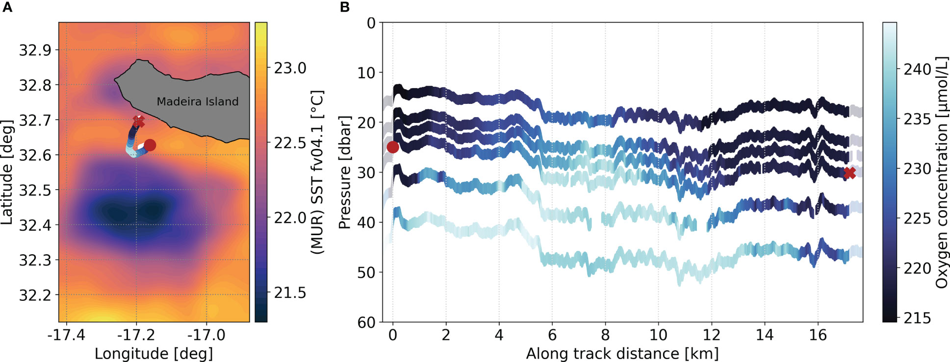
Figure 12 Oxygen concentration data collected with the TIA off Madeira Island, Portugal. A 125 m RTM TIA was operated on the 13 m motor yacht Dori. The ship track in panel (A) shows the oxygen concentrations in about 29 m depth, see also red markers in the data plot in panel (B). Gaps in the data plot indicate were data has been filtered out in post-processing due to insufficient data quality. The transect shown passes the edge of an incoming cyclonic eddy as indicated by the underlying sea surface temperature (MUR SST) data in panel (A). SST data is at 09:00 UTC, while TIA data has been collected between 11:04 and 13:50 UTC.

Panel (B) of Figure 12 proves TIAs capabilities to resolve submesoscale horizontal O₂-variability while providing an overview of the vertical structure of O₂-distribution, even with this reduced set of only 6 CTD+ probes. Given that oxygen is a key ocean health indicator, this shows that TIA is a suitable equipment to monitor the health of the upper ocean marine ecosystem.

5 Summary and conclusions

The Towed Instrument Array has been successfully developed to fill an observational gap in high resolution studies of the upper ocean and coastal areas. The TIA proved to be a lightweight, flexible and highly customisable instrument, suitable for a wide range of studies and vessels. We demonstrate the ability of the TIA to achieve horizontal resolutions of $\mathcal{O}$(10 m) up to $\mathcal{O}$(100 km) to resolve the submesoscale range and larger scale features appropriately. Based on the knowledge of the vertical hydrographic structure optimized vertical resolutions from less than 1 m to several 10 m can be adjusted flexibly. Given the equipment set-up, TIA’s main advantage with regards to submesoscale dynamics is to resolve horizontal buoyancy gradients. TIA’s measurements may be used concomitantly with ADCP measurements in order to estimate thermal-wind imbalance, as the difference between the vertical shear of the total velocity and the horizontal buoyancy gradient, thus providing the ageostrophic vertical shear.

The largest presented TIA setup can cover depths of about 100 m (section 4.1). With the recent availability of the TIA model (Deschner et al., 2023), forces and power requirements can be calculated in advance and drastically improve TIA setup considerations. Therefore we expect larger and deeper reaching TIA setups to emerge.

Design choices made for the TIA proved to be robust and reliable throughout several deployments with different setups, both in Real Time data-transmission Mode and Memory Mode. Both, the thin, high tensile strength, single conductor tow cable (RTM) or the Dyneema^® ropes (MM) contributed minor drag and therefore require small depressors to reach adequate depths. Standalone CTD+ probes with internal power supply can sample more than 24 h with one charge at about 6 to 7 Hz sample rate, providing enough battery capacity for long transects. Given a second set of CTD+ probes for exchange, continued sampling is possible within less than 1 h setup time. Data transmission via inductive coupling works reliably and provides real-time plots of the water column, suitable for adaptive sampling scenarios. With the TIA we introduce new types of sensors to the towed instrument chain concept, such as rapid, optical oxygen sensors or a variety of fluorometers. Other sensor types are technically possible, for example pH or turbidity sensors, and thus broadening the field of possible applications to study physical, chemical and biological interactions at high resolution in situ. Future technological improvements of the TIA could include an active depressor and higher data transmission rates in Real Time data-transmission Mode. An active depressor is under current development and will allow the TIA to follow the sea-floor, keep a steady depth or even to undulate. Additional work is needed to make the real-time data visualisation for adaptive sampling scenarios more user-friendly.

Together with the TIA, a software toolbox for data processing and quality control has been developed. Because the TIA combines numerous independent CTD+ probes operating on a vertical scale of about 100 m, the measurements need to have a high level of consistency between the probes. We show TIAs ability to reach and surpass required levels of accuracy and inter-sensor precision. Based on the work by Deschner et al. (2023) we could prove TIAs geo-reference accuracy to be well below the desired range of $\mathcal{O}$(10 m) even for long setups. That assures the correct positioning of the edges of submesoscale features at an accuracy of less than $\mathcal{O}$(10 m) and prevents the introduction of vertical artefacts in the ocean state variables. While the TIA processing package is working and usable, further efforts are needed to translate the MATLAB legacy code into a more accessible toolbox in an open language, add further processing functions like the sensor drift correction and migrate conversion functions to the TEOS-10 standard.

In section 4.2 we show an example where the TIA was used in Memory Mode by personnel without any previous experience with the system. Due to COVID19 restrictions, it was not possible for us to meet with and train the people on Tara, yet we reliably obtained a high quality TIA data set over the course more than one year, parts of which are published in Calil et al. (2023). The section 4.3 proves the usability of RTM-TIA on small boats with a low cost, minimalist winch setup. The examples provide proof that the presented TIA is simple, flexible, and robust enough, to be shipped to and used by scientific working groups around the globe potentially resulting in a much better understanding of the submesoscale processes in the upper ocean.

Data availability statement

The datasets presented in this study can be found in online repositories. The names of the repository/repositories and accession number(s) can be found below: Underlying datasets and scripts at Zenodo: https://doi.org/10.5281/zenodo.7708432, the dataset for Mission Microbiomes at Pangaea: https://doi.pangaea.de/10.1594/PANGAEA.953830.

Ethics statement

Written informed consent was obtained from the individual(s) for the publication of any potentially identifiable images or data included in this article.

Author contributions

TK wrote substantial parts of the manuscript and designed and coded the majority of the presented data evaluation studies and plots. BB built the first lightweight and modernized TIA prototype and initiated TIAs development. FW, TK, GS, SCD, MH, and BB were involved in instrument development and testing. RR, MH, PHRC, and TK designed, coded and tested the described TIA data processing packages, MH and RR curated all TIA data shown in the example results section using the TIA processing package. RR, SCD, and TK contributed substantial parts to the Tow Mechanics and Error Considerations sections. BB, PHRC, TK, and MH conceptualized and conducted the field work required for TIA development and example results section. BB and PHRC drove TIAs development by providing a variety of scientific use cases and acquiring funding. All authors contributed to the article and approved the submitted version.

Funding

The TIA development into the presented version was funded by the Helmholtz Association via the Helmholtz large investment initiative called ACROSS (2013-2017) and its successor MOSES (2017-2022), the Modular Observation Solutions for Earth Systems. Open access publication fees are funded by the library of Helmholtz-Zentrum Hereon.

Acknowledgments

We acknowledge the vast development efforts performed by Sea & Sun Technology GmbH that extended beyond the TIA development contract and thank Prof. Heinz Schelwat for his unlimited support. The Tara crew thankfully proved the concept of the TIA being eligible for vessels of opportunity. We gratefully acknowledge their efforts collecting high resolution data in remote locations. We like to thank especially Josep M. Erta, Guillaume Bourdin, and Thomas Linkowski for collecting and providing data. We thank Daniele Iudicone and Stéphane Pesant for taking the TIA to AtlantECO Mission Microbiomes. We acknowledge the efforts undertaken by our colleagues at OOM-ARDITI Madeira and the crew of DORI enabling the collection of the Madeira Island wake data set in 2022. MUR SST data were provided by JPL under support by NASA MEaSUREs program. Finally we like to acknowledge helpful contributions to the manuscript provided by Dr. Jana Hinners.

Conflict of interest

Author SCD declares that he was employed at the company Sea & Sun Technology GmbH during the time of instrument development. SCD declares no ongoing dependence with Sea & Sun Technology GmbH after changing to University of Kiel and therefore declares no conflict of interest during the time of writing. Authors FW and GS declare that they were employed at the company Sea & Sun Technology GmbH during the time of instrument development and writing of this paper. Sea & Sun Technology GmbH has been contracted by Helmholtz-Zentrum Hereon to develop the Towed Instrument Array.

The remaining authors declare that the research was conducted in the absence of any commercial or financial relationships that could be construed as a potential conflict of interest.

Publisher’s note

All claims expressed in this article are solely those of the authors and do not necessarily represent those of their affiliated organizations, or those of the publisher, the editors and the reviewers. Any product that may be evaluated in this article, or claim that may be made by its manufacturer, is not guaranteed or endorsed by the publisher.

Abbreviations

ADCP, Acoustic Doppler Current Profiler; Chl-A, Chlorophyll-A fluorescence; CTD, Conductivity-Temperature-Depth Instrument; GNSS, Global Navigation Satellite System; HTSC, Horizontal TIA Shape Correction; ICC, Inductive Coupling Clamp; M1, Intercalibration Method 1; M2, Intercalibration Method 2; MM, Memory Mode; NTP, Network Time Protocol; PLE, Probe Location Error; RTC, Real Time Clock; RTM, Real Time data-transmission Mode; SOG, Speed Over Ground; TIA, Towed Instrument Array; uCTD, underway CTD.

Footnotes

1. ^ https://www.sea-sun-tech.com/product/multiparameter-probe-ctd48-mc.
2. ^ www.amt-gmbh.com.
3. ^ see www.sea-sun-tech.com for data sheets.
4. ^ Mission Microbiomes is part of the AtlantECO Project funded by grant agreement No. 862923 of the European Union Horizon 2020 research and innovation programme, www.atlanteco.eu, https://fondationtaraocean.org/en/expedition/mission-microbiomes/.
5. ^ GGA - Global Positioning System Fix Data, Time, Position and fix related data.
6. ^ ZDA - Time and Date - UTC, day, month, year and local time zone.
7. ^ http://cfconventions.org/index.html.
8. ^ https://hereon-coast.atlassian.net/wiki/spaces/MG/overview.
9. ^ https://pythonhosted.org/seawater/eos80.html.
10. ^ Modular Observation Solutions for Earth Systems - https://www.helmholtz-klima.de/moses-modular-observation-solutions-earth-systems.
11. ^ https://www.hydrobios.de/en.
12. ^ http://www.atlanteco.eu.
13. ^ https://www.northlift.com/hydraulic-hauler-lh700.
14. ^ https://doi.org/10.5281/zenodo.5214122.

References

Adams K. A., Hosegood P., Taylor J. R., Sall J.-B., Bachman S., Torres R., et al. (2017). Frontal circulation and submesoscale variability during the formation of a southern ocean mesoscale eddy. J. Phys. Oceanogr. 47, 17. doi: 10.1175/JPO-D-16-0266.1

CrossRef Full Text | Google Scholar

Andrew R. K., Mercer J. A., Bell B. M., Ganse A. A., Buck L., Wen T., et al. (2010). “PhilSea10 APL-UW cruise report: 5–29 may 2010,” in Technical cruise reports APL-UW TR 1001 (Seattle, Washington: Applied Physics Laboratory, University of Washington).

Google Scholar

Azevedo C. C., Camargo C. M. L., Alves J., Caldeira R. M. A. (2021). Convection and heat transfer in island (Warm) wakes. J. Phys. Oceanogr. 51, 1187–1203. doi: 10.1175/JPO-D-20-0103.1

CrossRef Full Text | Google Scholar

Baschek B. (2002). Air-Sea gas exchange in tidal fronts (Canada: School of Earth and Ocean Sciences - University of Victoria).

Google Scholar

Baschek B., Farmer D. M., Garrett C. (2006). Tidal fronts and their role in air-sea gas exchange. J. Mar. Res. 64, 483–515. doi: 10.1357/002224006778715766

CrossRef Full Text | Google Scholar

Baschek B., Jenkins W. J. (2009). Gas ventilation of the saguenay fjord by an energetic tidal front. Atmosphere-Ocean 47, 308–318. doi: 10.3137/OC314.2009

CrossRef Full Text | Google Scholar

Baschek B., Schroeder F., Brix H., Riethmüller R., Badewien T. H., Breitbach G., et al. (2017). The coastal observing system for northern and Arctic seas (COSYNA). Ocean Sci. 13, 379–410. doi: 10.5194/os-13-379-2017

CrossRef Full Text | Google Scholar

Brown J., Brander K., Fernand L., Hill A. E. (1997). Scanfish: high performance towed undulator. Oceanographic Literature Rev. 5, 523.

Google Scholar

Caldeira R. M. A., Groom S., Miller P., Pilgrim D., Nezlin N. P. (2002). Sea-Surface signatures of the island mass effect phenomena around Madeira island, northeast Atlantic. Remote Sens. Environ. 80, 336–360. doi: 10.1016/S0034-4257(01)00316-9

CrossRef Full Text | Google Scholar

Calil P., Riethmüller R., Kock T., Heineke M., Iudicone D., Pesant S., et al. (2023). Data of towed instrument array (TIA) during the mission microbiomes with the RV Tara on two transects in Amazon plume region (Geesthacht, Germany: Helmholtz-Zentrum). doi: 10.1594/PANGAEA.953830

CrossRef Full Text | Google Scholar

Calil P. H. R., Suzuki N., Baschek B., da Silveira I. C. A. (2021). Filaments, fronts and eddies in the cabo frio coastal upwelling system, Brazil. Fluids 6, 54. doi: 10.3390/fluids6020054

CrossRef Full Text | Google Scholar

Capet X., McWilliams J. C., Molemaker M. J., Shchepein A. F. (2008). Mesoscale to submesoscale transition in the California current system. part I: flow structure, eddy flux, and observational tests. J. Phys. Oceanogr. 38, 29–43. doi: 10.1175/2007JPO3671.1

CrossRef Full Text | Google Scholar

Carpenter J. R., Rodrigues A., Schultze L. K. P., Merckelbach L. M., Suzuki N., Baschek B., et al. (2020). Shear instability and turbulence within a submesoscale front following a storm. Geophysical Res. Lett. 47, e2020GL090365. doi: 10.1029/2020GL090365

CrossRef Full Text | Google Scholar

Chapman D. A. (1984). Towed cable behaviour during ship turning manoeuvers. Ocean Eng. 11, 327–361. doi: 10.1016/0029-8018(84)90010-6

CrossRef Full Text | Google Scholar

Chrysagi E., Umlauf L., Holtermann P., Klingbeil K., Burchard H. (2021). High-resolution simulations of submesoscale processes in the Baltic Sea: the role of storm events. J. Geophys. Res. Oceans 126. doi: 10.1029/2020JC016411

CrossRef Full Text | Google Scholar

D’Asaro E., Lee C., Rainville L., Harcourt R., Thomas L. (2011). Enhanced turbulence and energy dissipation at ocean fronts. Science 332, 318–322. doi: 10.1126/science.1201515

PubMed Abstract | CrossRef Full Text | Google Scholar

de Boyer Montégut C., Madec G., Fischer A. S., Lazar A., Iudicone D. (2004). Mixed layer depth over the global ocean: an examination of profile data and a profile-based climatology. J. Geophys. Res. Oceans 109. doi: 10.1029/2004JC002378

CrossRef Full Text | Google Scholar

Deschner S. C., Kock T., Schelwat H., Baschek B. (2023). Submerged marine towed instrument array: a theoretical investigation using Lagrange mechanics. Ocean Eng. 267, 113201. doi: 10.1016/j.oceaneng.2022.113201

CrossRef Full Text | Google Scholar

Dever M., Freilich M., Farrar J. T., Hodges B., Lanagan T., Baron A. J., et al. (2020). EcoCTD for profiling oceanic physical–biological properties from an underway ship. J. Atmos Oceanic Technol. 37, 825–840. doi: 10.1175/JTECH-D-19-0145.1

CrossRef Full Text | Google Scholar

Farmer D., Armi L. (1999). Stratified flow over topography: the role of small-scale entrainment and mixing in flow establishment. Proc. R. Soc London Ser. A 455, 3221–3258. doi: 10.1098/rspa.1999.0448

CrossRef Full Text | Google Scholar

Farmer D. M., D’asaro E. A., Trevorrow M. V., Dairiki G. T. (1995). Three-dimensional structure in a tidal convergence front. Continental Shelf Res. 15, 1649–1673. doi: 10.1016/0278-4343(94)00084-Z

CrossRef Full Text | Google Scholar

Ferrari R., Rudnick D. L. (2000). Thermohaline variability in the upper ocean. J. Geophysical Research: Oceans 105, 16857–16883. doi: 10.1029/2000JC900057

CrossRef Full Text | Google Scholar

Floeter J., van Beusekom J. E. E., Auch D., Callies U., Carpenter J., Dudeck T., et al. (2017). Pelagic effects of offshore wind farm foundations in the stratified north Sea. Prog. Oceanography 156, 154–173. doi: 10.1016/j.pocean.2017.07

CrossRef Full Text | Google Scholar

Fofonoff N., Millard R. (1983). “Algorithms for computation of fundamental properties of seawater. endorsed by Unesco/SCOR/ICES/IAPSO joint panel on oceanographic tables and standards and SCOR working group 51,” in Unesco technical papers in marine science, no. 44 (Paris, France: UNESCO).

Google Scholar

Fox-Kemper B., Ferrari R. (2008). Parameterization of mixed layer eddies. part II: prognosis and impact. J. Phys. Oceanography 38, 1166–1179. doi: 10.1175/2007JPO3788.1

CrossRef Full Text | Google Scholar

Furlong A., Beanlands B., Chin-Yee M. (1997)Moving vessel profiler (MVP) real time near vertical data profiles at 12 knots (Accessed Oceans ‘97. MTS/IEEE Conference Proceedings).

Google Scholar

Ginzkey L. (1977). Der leitfähigkeitssensor der kieler multisonde für in situ-messungen der spezifischen elektrischen leitfähigkeit (Kiel, Germany: Christian-Albrechts-Universität zu Kiel).

Google Scholar

Grosenbaugh M. A. (2007). Transient behavior of towed cable systems during ship turning maneuvers. Ocean Eng. 34, 1532–1542. doi: 10.1016/j.oceaneng.2007.01.002

CrossRef Full Text | Google Scholar

JPL MUR MEaSUREs Project (2015). GHRSST level 4 MUR global foundation Sea surface temperature analysis (v4.1) (California, USA: NASA physical oceanography DAAC).

Google Scholar

Kaplan E. D., Hegarty C. (2006). Understanding GPS: principles and applications. 2nd ed (Boston: Artech House).

Google Scholar

Kock T., Baschek B., Wobbe F., Heineke M., Riethmüller R., Deschner S. C., et al. (2023). Dataset and scripts for reproducing figures and analyses used in “An advanced towed CTD chain for physical-biological high resolution in situ ocean surface measurements. doi: 10.5281/zenodo.7708432

PubMed Abstract | CrossRef Full Text | Google Scholar

Körtzinger A., Andrae A., Baschek B., Becker K., Behr H.-D., Blandfort D., et al. (2020). Eddy study to understand physical-Chemical-Biological coupling and the biological carbon pump as a function of eddy type off West Africa, cruise no. M160, 23.11.2019 - 20.12.2019, mindelo (Cabo Verde) - mindelo (Cabo Verde) (Bonn: Gutachterpanel Forschungsschiffe). doi: 10.2312/cr_m

CrossRef Full Text | Google Scholar

Lévy M., Ferrari R., Franks P. J. S., Martin A. P., Rivière P. (2012). Bringing physics to life at the submesoscale: FRONTIER. Geophys. Res. Lett. 39. doi: 10.1029/2012GL052756

PubMed Abstract | CrossRef Full Text | Google Scholar

Lévy M., Franks P. J. S., Smith K. S. (2018). The role of submesoscale currents in structuring marine ecosystems. Nat. Commun. 9, 4758. doi: 10.1038/s41467-018-07059-3

PubMed Abstract | CrossRef Full Text | Google Scholar

Lips I., Lips U., Fleming V., Kaitala S., Jaanus A. (2006). Use of ferrybox measurements for the Baltic Sea environment assessment (IEEE). Environmental Research, Engineering and Management 3 (41), 7. doi: 10.1109/BALTIC.2006.7266159

CrossRef Full Text | Google Scholar

Lund B., Haus B. K., Horstmann J., Graber H. C., Carrasco R., Laxague N. J. M., et al. (2018). Near-surface current mapping by shipboard marine X-band radar: a validation. J. Atmospheric Oceanic Technol. 35, 1077–1090. doi: 10.1175/JTECH-D-17-0154.1

CrossRef Full Text | Google Scholar

Mahadevan A. (2016). The impact of submesoscale physics on primary productivity of plankton. Annu. Rev. Mar. Sci. 8, 161–184. doi: 10.1146/annurev-marine-010814-015912

CrossRef Full Text | Google Scholar

Mahadevan A., Tandon A. (2006). An analysis of mechanisms for submesoscale vertical motion at ocean fronts. Ocean Model. 14, 241–256. doi: 10.1016/j.ocemod.2006.05.006

CrossRef Full Text | Google Scholar

McDougall T. J., Barker P. M. (2011). Getting started with TEOS-10 and the Gibbs seawater (GSW) oceanographic toolbox (Maryland USA: SCOR/IAPSO WG127), ISBN: ISBN 978-0-646-55621-5.

Google Scholar

McWilliams J. C. (2016). Submesoscale currents in the ocean. Proc. R. Soc A 472, 20160117. doi: 10.1098/rspa.2016.0117

CrossRef Full Text | Google Scholar

McWilliams J. C., Molemaker M. J. (2011). Baroclinic frontal arrest: a sequel to unstable frontogenesis. J. Phys. Oceanography 41, 601–619. doi: 10.1175/2010JPO4493.1

CrossRef Full Text | Google Scholar

Mobley F., Sadilek A., Gundersdorf C., Speranza D. (1976). A new thermistor chain for underwater temperature measurement. OCEANS 76, 529–536. doi: 10.1109/OCEANS.1976.1154280

CrossRef Full Text | Google Scholar

Olivier L., Reverdin G., Boutin J., Laxenaire R., Iudicone D., Pesant S., et al. (2022). Late summer northwestward Amazon plume pathway under the action of the north Brazil current rings (Washington D.C.: AGU JGR oceans).

Google Scholar

Omta A. W., Kooijman S. A. L. M., Dijkstra H. A. (2008). Critical turbulence revisited: the impact of submesoscale vertical mixing on plankton patchiness. J. Mar. Res. 66, 61–85. doi: 10.1357/002224008784815766

CrossRef Full Text | Google Scholar

Osiński R., Rak D., Walczowski W., Piechura J. (2010). Baroclinic rossby radius of deformation in the southern Baltic Sea. OCEANOLOGIA 52, 417–429. doi: 10.5697/oc.52-3.417

CrossRef Full Text | Google Scholar

Petersen W., Reinke S., Breitbach G., Petschatnikov M., Wehde H., Thomas H. (2018). FerryBox data in the north Sea from 2002 to 2005. Earth System Sci. Data 10, 1729–1734. doi: 10.5194/essd-10-1729-2018

CrossRef Full Text | Google Scholar

Pidcock R., Srokosz M., Allen J., Hartman M., Painter S., Mowlem M., et al. (2010). A novel integration of an ultraviolet nitrate sensor on board a towed vehicle for mapping open-ocean submesoscale nitrate variability. J. Atmospheric Oceanic Technol. 27, 1410–1416. doi: 10.1175/2010JTECHO780.1

CrossRef Full Text | Google Scholar

Pollard R. (1986). Frontal surveys with a towed profiling conductivity/temperature/depth measurement package (SeaSoar). Nature 323, 433–435. doi: 10.1038/323433a0

CrossRef Full Text | Google Scholar

Richardson W. S., Hubbard C. J. (1959). The contouring temperature recorder. Deep Sea Res. 6, 239–244. doi: 10.1016/0146-6313(59)90078-4

CrossRef Full Text | Google Scholar

Rowe F., Young J. (1979). An ocean current profiler using Doppler sonar. OCEANS 79, 292–297. doi: 10.1109/OCEANS.1979.1151265

CrossRef Full Text | Google Scholar

Rudnick D. L., Ferrari R. (1999). Compensation of horizontal temperature and salinity gradients in the ocean mixed layer. Science 283, 526–529. doi: 10.1126/science.283.5401.526

PubMed Abstract | CrossRef Full Text | Google Scholar

Rudnick D. L., Klinke J. (2007). The underway conductivity–Temperature–Depth instrument. J. Atmospheric Oceanic Technol. 24, 1910–1923. doi: 10.1175/JTECH2100.1

CrossRef Full Text | Google Scholar

Salm K., Liblik T., Lips U. (2023). Submesoscale variability in a mesoscale front captured by a glider mission in the gulf of Finland, Baltic Sea. Front. Mar. Sci. 10. doi: 10.3389/fmars.2023.984246

CrossRef Full Text | Google Scholar

Sanborn B., DiLeonardi A. M., Weerasooriya T. (2015). Tensile properties of dyneema SK76 single fibers at multiple loading rates using a direct gripping method. J. Dynamic Behav. Mater. 1, 4–14. doi: 10.1007/s40870-014-0001-3

CrossRef Full Text | Google Scholar

SeaDataNet (2017). Quality control standards for SEADATANET. (Brest, France: IFREMER)

Google Scholar

Sellschopp J. (1997). A towed CTD chain for two-dimensional high resolution hydrography. Deep Sea Res. Part I: Oceanographic Res. Papers 44, 147–165. doi: 10.1016/S0967-0637(96)00087-8

CrossRef Full Text | Google Scholar

Sellschopp J., Arneborg L., Knoll M., Fiekas V., Gerdes F., Burchard H., et al. (2006). Direct observations of a medium-intensity inflow into the Batic Sea. Continental Shelf Res. 26, 2393–2414. doi: 10.1016/j.csr.2006.07.004

CrossRef Full Text | Google Scholar

Sellschopp J., Nielsen P., Siderius M. (2002). “Combination of acoustics with high resolution oceanography,” in Impact of littoral environmental variability of acoustic predictions and sonar performance. Eds. Pace N. G., Jensen F. B. (Dordrecht: Springer Netherlands), 19–26. doi: 10.1007/978-94-010-0626-2_3

CrossRef Full Text | Google Scholar

Spall M. A. (1995). Frontogenesis, subduction, and cross-front exchange at upper ocean fronts. J. Geophys. Res. 100, 2543. doi: 10.1029/94JC02860

CrossRef Full Text | Google Scholar

Tedford E. W., Carpenter J. R., Pawlowicz R., Pieters R., Lawrence G. A. (2009). Observation and analysis of shear instability in the Fraser river estuary. J. Geophysical Research: Oceans 114. doi: 10.1029/2009JC005313

CrossRef Full Text | Google Scholar

Thomas L. N., Tandon A., Mahadevan A. (2008). Submesoscale processes and dynamics. Gephysical Monograph Ser. 177, 22. doi: 10.1029/177GM04

CrossRef Full Text | Google Scholar

Velasco D. W., Nylund S., Pettersen T. (2018). “Combined current profiling and biological echosounding results from a single ADCP,” in 2018 OCEANS - MTS/IEEE Kobe techno-oceans (OTO) (Kobe: IEEE), 1–5. doi: 10.1109/OCEANSKOBE.2018.8559356

CrossRef Full Text | Google Scholar

Weber U., Attinger S., Baschek B., Boike J., Borchardt D., Brix H., et al. (2021). MOSES: a novel observation system to monitor dynamic events across earth compartments. Bull. Am. Meteorol Soc. -1, 1–23. doi: 10.1175/BAMS-D-20-0158.1

CrossRef Full Text | Google Scholar

Wilkinson M. D., Dumontier M., Aalbersberg I. J., Appleton G., Axton M., Baak A., et al. (2016). The FAIR guiding principles for scientific data management and stewardship. Sci. Data 3, 160018. doi: 10.1038/sdata.2016.18

PubMed Abstract | CrossRef Full Text | Google Scholar