Calibration of fish counts in video surveys: a case study from the Southeast Reef Fish Survey

Introduction

Estimating the abundance of marine fish or invertebrates over large spatial or temporal scales is typically accomplished with data from scientific surveys, and these abundance estimates or indices are critically informative inputs to stock assessments (Dennis et al., 2015; Maunder and Piner, 2015). A wide variety of sampling gears have been used by scientific surveys to estimate fish abundance (Murphy and Jenkins, 2010; Goethel et al., 2022). Trawls are typically used on unconsolidated sediments and can often be used to estimate absolute abundance or density of fish given the known area sampled (Kimura and Somerton, 2006). On untrawlable habitats like natural or artificial reefs, numerous gears have been used but the resulting abundance estimates are often relative (i.e., indices of abundance) because estimating the area over which sampling occurs is challenging (Maunder and Punt, 2004; Bacheler et al., 2022a). It is nearly universally assumed that indices of abundance from survey data vary in proportion to the actual abundance of the population; in other words, catchability (i.e., the efficiency of a sampling gear) is nearly always assumed to be constant over space and time, even though its absolute value is generally unknown (Hangsleben et al., 2013).

There are several reasons why catchability of a survey gear may not be constant over time. Catchability is often considered to be the product of availability (i.e., proportion of the stock occurring in the survey area) and gear efficiency (i.e., the proportion of animals caught or detected that are available to the gear; Arreguín-Sánchez (1996)). Changes in the spatial footprint of a survey or seasonal or diurnal migrations of a species of interest influence that species’ availability to the survey (Aguzzi and Company, 2010). Moreover, environmental variability can influence the efficiency of sampling gears (Bacheler et al., 2014; Bacheler and Shertzer, 2020), which, if left unaccounted for, will be confounded with temporal trends in abundance (Tyre et al., 2003). Another reason why catchability can vary in a survey is due to changes in gears, vessels, or sampling characteristics over time (Pelletier, 1998; Cadigan and Dowden, 2010; Thorson and Ward, 2014). These changes may be unavoidable (e.g., when a survey vessel or outdated equipment needs to be replaced), while other changes may be discretionary (e.g., due to improved performance or ease of use of new gears). Regardless, any of these changes require calibration between the old and new sampling methodologies because any change in gears or vessels can influence the relative catch rates (Pelletier, 1998; Kimura and Somerton, 2006).

Over the last few decades, underwater video has become a common tool for indexing the abundance and distribution of fish species in many places throughout the world (Mallet and Pelletier, 2014; Whitmarsh et al., 2017; Bacheler and Ballenger, 2018). Underwater video has evolved into a valuable sampling gear that can be standardized to provide indices of abundance for a wide variety of pelagic and demersal fish species (Priede and Merrett, 1996; Heagney et al., 2007; Brooks et al., 2011; Santana-Garcon et al., 2014; Bacheler and Ballenger, 2018). Some video surveys use unbaited cameras while others are baited, and different fish communities may be sampled based on bait choices (Harvey et al., 2007; Dorman et al., 2012).

While improvements have been made to most sampling gears over time, underwater video cameras have evolved particularly dramatically over the last half century (Mallet and Pelletier, 2014). The original cameras used to quantify fish species diversity and abundance were large (~ 1 m high, 0.5 m in diameter), low quality, and needed a connection to a power supply on land or ship (Kumpf and Lowenstein, 1962; Myrberg et al., 1969). Nowadays, underwater video cameras are small, cheap, reliable, fully digital, record in high definition, and have small and long-lasting batteries (Struthers et al., 2015). Just as changes to trawl nets or the vessels dragging them influence the catchability of fish, the improvements of video cameras over time likely improved the sightability of fish (i.e., ability to see fish that are present). Even within the advanced underwater video cameras available today, there is enormous variability in video size, shape, color, quality, and light sensitivity that can influence the sightability of fish. Despite the vast changes in video cameras over time and the fact that numerous fishery-independent surveys use video cameras, there are few published examples where fish counts have been calibrated between cameras (but note that calibrations commonly occur when measuring fish length; Harvey and Shortis, 1998; Balletti et al., 2014; Letessier et al., 2015; Shafait et al., 2017).

Here, we describe a calibration study that was undertaken to account for a camera change in the Southeast Reef Fish Survey (SERFS), a large-scale fishery-independent trap and video survey that provides key relative abundance data for many reef-associated fish species along the southeast United States Atlantic coast (hereafter, SEUS) between North Carolina and Florida. There were four objectives of our work. The first objective was to describe the statistical design and methodological approach of our calibration experiment with paired camera given the paucity of examples in the literature. Our second objective was to estimate species-specific calibration factors for multiple economically important reef fish species in the SEUS. Our third objective was to consider alternatives to species-specific calibrations when sample sizes were limited, for instance, by borrowing information from related or unrelated species. The fourth objective was to evaluate two approaches for applying calibration factors between video cameras: calibrating the data before inclusion in a standardization model or after standardization has occurred (i.e., calibrating the index itself). Through this case study, we describe the importance of video calibrations, detail the lessons learned from our video calibration experiment, and provide guidance to researchers around the world on how to calibrate for changes in video sampling gears.

Materials and methods

Objective 1: calibration experiment design

Video data for this study were provided by SERFS, a regional-scale trap and video survey occurring in the SEUS. SERFS is made up of three groups that sample reef fish species collaboratively using identical methods. The first group is the Marine Resources Monitoring, Assessment, and Prediction program, housed at the South Carolina Department of Natural Resources, which has been funded by the National Marine Fisheries Service (NMFS) to sample with chevron traps in the region since 1990. The second group is the Southeast Area Monitoring and Assessment Program – South Atlantic Region reef fish complement, which has provided additional funding to South Carolina Department of Natural Resources to conduct reef fish surveys in the region since 2009. The third group is the Southeast Fishery-Independent Survey, which was created by NMFS in 2010 to work with their partners listed above to increase fishery-independent sample sizes in the SEUS and incorporate underwater video into the survey.

SERFS used a simple random sampling design to select stations for sampling each year. Approximately 2,000 stations were randomly selected for sampling each year out of a sampling frame of approximately 4,300 stations on known hardbottom reef habitat. A majority of stations sampled each year and included in our analyses were randomly selected for sampling, but some stations not selected for sampling were sampled opportunistically to increase sampling efficiency. A small number of new hardbottom sampling stations were discovered and sampled each year, and were included in our analyses if hardbottom was observed on video. Sampled stations were always separated by at least 200 m in a given year to provide independence between samples. Five research vessels have been used to carry out this work: the R/V Palmetto, R/V Savannah, NOAA Ship Nancy Foster, NOAA Ship Pisces, and NOAA Ship SRVx Sand Tiger. All video sampling occurred during daylight hours between the spring and fall each year.

For 20 years, SERFS used chevron traps alone to sample reef fish species in the SEUS. Chevron traps are large, arrowhead-shaped traps that were baited with Brevoortia spp. and soaked for ~90 min (Figure 1). Beginning in 2011, all chevron traps deployed by SERFS included two attached cameras – one placed over the trap mouth that looked outward and used to count fish and quantify seafloor habitat, and one placed over the trap nose that also looked outward, but this second camera was only used to quantify seafloor habitat in the opposite direction of the first camera. In 2011–2014, Canon Vixia HF-S200 video cameras in Gates HF-21 housings were attached over the mouth of the trap and used to count fish. In 2015, GoPro Hero 3+ cameras replaced the Canon cameras because GoPros are smaller, cheaper, higher resolution, and have a larger field of view, which we expected would increase fish counts relative to Canon cameras (Figure 2).

FIGURE 1

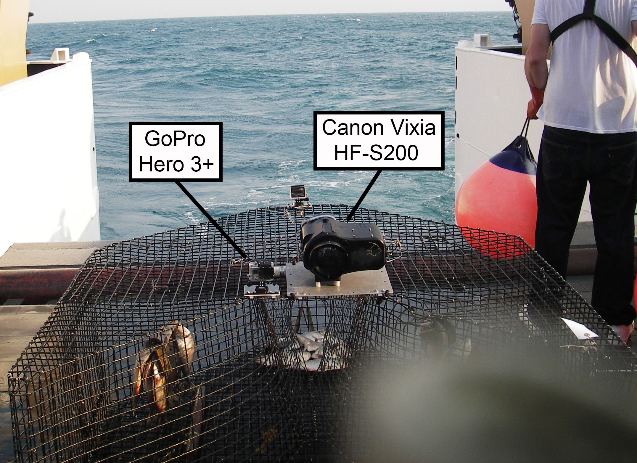
Figure 1 Side-by-side calibration experiment conducted by the Southeast Reef Fish Survey along the southeast United States Atlantic coast in 2014. Canon Vixia HF-S200 and GoPro Hero 3+ cameras were attached to baited traps side-by-side looking outward and read for fish at exactly the same times using the MeanCount approach (Schobernd et al., 2014).

FIGURE 2

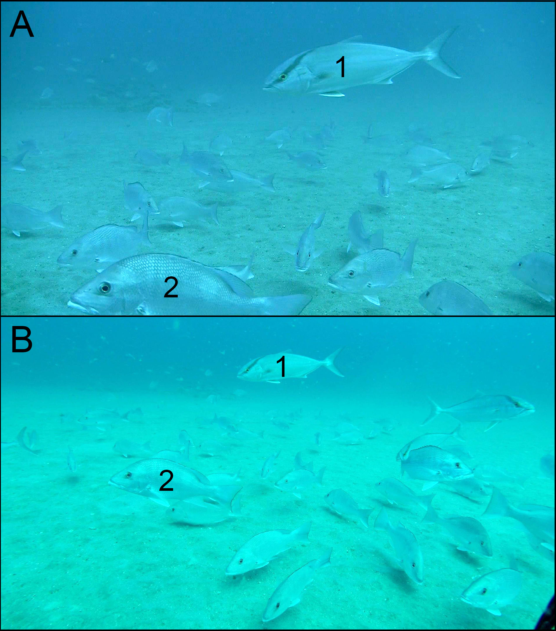
Figure 2 Differences in field of view between two underwater video cameras, paired in space and time, from a sample of the Southeast Reef Fish Survey off Jacksonville, Florida, taken in 2014. (A) Image from a Canon^® Vixia HF-S200 video camera in Gates underwater housing. (B) Image from GoPro Hero 3+ camera in stock underwater housing. Numbers are shown so readers can identify and compare the same individual fish in each image: (1) almaco jack Seriola rivoliana; (2) red snapper Lutjanus campechanus.

To address our first objective and account for this camera switch, we conducted a calibration experiment during the 2014 field season. We attached Canon Vixia HF-S200 and GoPro Hero 3+ cameras side-by-side on traps, looking outward over the trap mouth (Figures 1, 2). In addition to pairing video cameras in space, we also paired video reading in time (see below). A total of 143 chevron traps were deployed in 2014 that included both video cameras placed side-by-side over trap mouths, looking outward. Two video cameras malfunctioned, leaving 141 paired video samples that were available for reading. Of these, 54 paired samples were deemed to have sufficient numbers of priority fish species (e.g., red snapper) from cursory examinations to make complete reading of these calibration videos worthwhile.

Objective 2: estimating calibrations for reef fish species

We focused our analyses on economically-important species of reef fish species across various families that had sufficient calibration sample sizes (minimum sample size threshold: N ≥ 4). Note that two species of lionfish Pterois spp. (i.e., devil firefish Pterois miles and red lionfish Pterois volitans) exist in the SEUS and are difficult to distinguish visually (Hamner et al., 2007), so they were treated as a single species here.

All videos were read using the MeanCount approach, which was calculated as the mean number of individuals of a particular species that was observed in a series of snapshots within a video (Schobernd et al., 2014). Schobernd et al. (2014) showed that MeanCount was proportional to actual abundance using laboratory, simulation, and field data, while other common video reading metrics like MaxN (i.e., MinCount; Ellis and DeMartini, 1995) were often nonlinearly related to actual abundance (but see Campbell et al., 2018). Here, we followed SERFS video reading protocol: all species were counted on a total of 41 snapshots, starting 10 min after the trap landed on the bottom and spaced 30 seconds apart for a total of 20 min (Bacheler et al., 2020). Four video readers with extensive training in fish identification read these calibration videos, and a portion of videos from each reader were read by other readers to ensure accuracy.

Species-specific calibration factors were estimated using linear models. Linear models related the MeanCounts of a particular species on Canon cameras (MeanCount_Canon) as the response variable to the counts of that species on GoPro cameras (MeanCount_GoPro) as the predictor variable as follows:

$\begin{array}{ll}{\text{MeanCount}}_{Canon}=a+b({\text{MeanCount}}_{GoPro})& (1)\end{array}$

where a is the model intercept and b is the slope. We also provide the R² value for each model, which indicates how predictable Canon counts are from GoPro counts. Note that we are using Canon counts as the response variable and GoPro counts as the predictor variable here, implying that our slope and intercept estimates would be used to reduce GoPro counts to make them comparable to Canon counts (see Results below). Alternatively, we could have used GoPro counts as the response variable and Canon counts as the predictor variable, in which case slope and intercept estimates would be used to increase Canon counts to make them comparable to GoPro counts. Ultimately, we are interested in using these data to develop time series of relative abundance, which were robust to the direction of calibration. These and all following analyses were conducted in R (R Core Team, 2021).

Objective 3: limited sample sizes

Calibrations for species with relatively low sample sizes were in some cases poorly estimated (see Results below), so our third objective was to evaluate whether borrowing information from related or unrelated species might be warranted in some cases. Ideally, sufficient data will be collected for all species of interest during calibration experiments, but in our case, despite collecting 143 paired calibration videos, some important but rare species had quite low sample sizes.

One potential solution for estimating calibrations for species with low sample sizes is to apply an overall calibration calculated across all species. This approach would only be justified if variability among families was low. To evaluate whether this was the case, we calculated family-level calibrations for each of the family groupings in our calibration dataset, using linear models as described in Equation 1 above. Similar calibrations among families would suggest low variability among taxa and therefore an overall calibration might be substituted for species with low sample sizes. Alternatively, significant variability among families would suggest applying an overall calibration to taxa would not be valid. Note that commonly observed species will tend to drive family-level calibrations much more so than rarer species.

Another possible solution is to apply the family-level calibrations to species with low sample sizes. In this situation, there may be behavioral or anatomical similarities among species of a particular family that could justify borrowing information from related species. For families containing more than one species with sufficient calibration sample sizes, we compared family-level calibrations to those of each species within that family. Similar calibrations for species within a family might justify the use of a family-level calibration for species with insufficient sample sizes. In contrast, if there is sufficient variability in calibrations among species within a family, applying a family-level calibration to any particular species is likely not justified.

Objective 4: compare approaches to apply calibrations when developing indices of relative abundance

Our fourth objective was to evaluate two approaches for applying calibrations: calibrating the data before inclusion into a standardization model or after standardization has occurred. Calibrating at the data level would be preferable in various situations where standardization models are not being used, for example, in ecological studies or specific research projects. Alternatively, calibrating a final index of abundance is much faster and easier and would be preferable in most cases where video data are being standardized with a statistical model. It was unclear, however, if these two methods of applying calibrations provided standardized indices of abundance that are equivalent.

To evaluate this objective, we tested whether indices of abundance from two representative species varied based on how the calibrations were applied (i.e., at the data or index level). We used SERFS video data in 2011–2021 for scamp Mycteroperca phenax and red snapper Lutjanus campechanus. These species were selected because they have displayed opposite patterns in relative abundance during the 2011–2021 time frame, with red snapper increasing (SEDAR, 2021a) and scamp declining (SEDAR, 2021b).

Here we followed the standardization procedures used for SERFS video data in the stock assessments of these two species (SEDAR, 2021a; SEDAR, 2021b). The response variable was SumCount, defined as the total number of individuals (scamp or red snapper) observed across all frames of a unique video sampling event. For these analyses, SumCount was used instead of MeanCount because the negative binomial distribution operates on discrete variables (MeanCount is continuous), but we note that SumCount relates linearly to MeanCount because the number of frames per event is constant. The distribution of SumCount for most species contained a large proportion of zeros and had an extended tail of positive values. Therefore, the modeling approach applied a zero-inflated negative binomial (ZINB) formulation, in which a negative binomial sub-model describes the count data and a binomial sub-model describes the occurrence of positive versus zero counts (Zeileis et al., 2008; Zuur et al., 2009). Explanatory variables included year (y), season (t), depth (d), latitude (lat), temperature (temp), water clarity (wc), current direction (cd), biotic density (bd), and substrate composition (sc; see Bacheler et al. (2014) for details). Year was necessarily included, because for an index of abundance, the year effect is of primary interest. The other variables were included or excluded based on a step-wise backward model selection procedure, starting with the full model formulation and then removing variables that did not contribute to explaining variance in the data, based on the Akaike information criterion (AIC) and likelihood ratio tests (Zuur et al., 2009). For this procedure, the initial full model was:

$\begin{array}{ll}\begin{array}{l}SumCount=y+t+d+lat+temp+wc+cd+bd+sc |\\ y+t+d+lat+temp+wc+cd+bd+sc.\end{array}& (2)\end{array}$

In this formulation, variables to the left of the vertical bar apply to the negative binomial sub-model and variables below it apply to the binomial sub-model. The final model included only those variables that were retained after applying the model selection procedure. Model fitting used the zeroinfl function in the countreg package of R (Zeileis and Kleiber, 2017).

Uncertainty in the resulting index of abundance was computed using a bootstrap procedure with N = 1000 replicates. For each replicate, a new data set of the original size was created by drawing video observations (rows) at random with replacement. The final model configuration was fitted to each replicate data set, and resulting variability (i.e., 95% confidence intervals) in the relative abundance was computed for each year.

The calibration method was applied in two different ways, either at the index level or the data level. To calibrate at the index level, the index was first computed from the original, uncalibrated data. Then, the species-specific linear model (Equation 1) was applied to the standardized index for years 2015 and onward. To account for uncertainty in the calibration itself, parameters of the linear model were included as part of the bootstrap process described above. This was accomplished by drawing at random a new intercept and slope for each bootstrap iteration, in which each draw came from a bivariate normal distribution with means equal to the parameter point estimates and the covariance matrix as estimated by the linear regression. For both species, the point estimate of the intercept was negative, which is expected given that GoPro cameras have a wider field of view and therefore more fish should be observed on GoPros than on Canons. Thus, to preserve that feature in the bootstrap procedure, we truncated the bivariate distribution to provide only negative intercept values.

To calibrate at the data level, the data themselves were adjusted prior to fitting the models. For each positive observation of SumCount in 2015-2021 in the original data, a calibrated SumCount value was drawn from a binomial distribution, $B(n_i, p_i)$. Here, n_i is the original SumCount for observation i, and p_i was determined by the linear regression (Equation 1) as:

$\begin{array}{ll}{p}_i=(a+b{n}_i)/n_i& (3)\end{array}$

In the bootstrap process, uncertainty in the regression parameters (a and b) were incorporated using the same bivariate normal distribution as in the index-level calibration. The index was fitted to each calibrated data set, but the final index did not require any adjustment.

Results

Objective 1: calibration experiment design

A total of 27 fish species were observed and counted across the 54 calibration videos collected in 2014. The most commonly observed species on calibration videos was gray triggerfish Balistes capriscus (N = 41 videos), followed by vermilion snapper Rhomboplites aurorubens (N = 40), red snapper (N = 31), and black sea bass Centropristis striata (N = 28; Table 1). The least commonly observed species among those included in our analyses were red grouper Epinephelus morio (N = 4), mutton snapper Lutjanus analis (N = 6), and hogfish Lachnolaimus maximus (N = 8). Eleven fish species were counted on calibration videos but excluded from all analyses because they did not reach the minimum sample size threshold.

TABLE 1

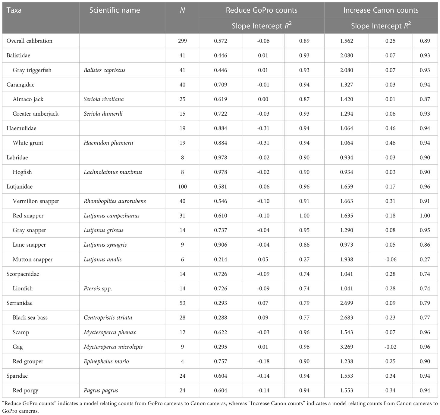
Table 1 Calibration information for the 16 reef fish species with a sample size (N) of at least 4, their associated families, and a fit across all 16 species (“overall calibration”) as part of the 2014 side-by-side calibration study by the Southeast Reef Fish Survey along the southeast United States Atlantic coast.

Objective 2: estimating calibrations for reef fish species

Sixteen species met our minimum sample size threshold of being observed on at least 4 calibration videos, and calibrations were variable among these species (Table 1; Figure 3). Slope estimates ranged from 0.214 for mutton snapper to 0.978 for hogfish, but 8 of 16 species and generally those species with the largest sample sizes had slope estimates within a fairly narrow range of 0.440 to 0.740 (Table 1). The slope of the overall model that included all 16 species was 0.572, suggesting that, on average, 42.8% fewer fish were observed on Canon compared to GoPro cameras. Species-specific model intercepts ranged from -0.31 (white grunt Haemulon plumierii) to 0.09 (black sea bass), with 11 of 16 being negative as expected given we are calibrating a camera that observed more fish (i.e., GoPro) to a camera that observed fewer fish (i.e., Canon; Table 1). All but one species-specific R² value was greater than 0.70, and 11 of 16 were at least 0.90, suggesting GoPro counts predicted Canon counts well for most species (Table 1; Figure 3).

FIGURE 3

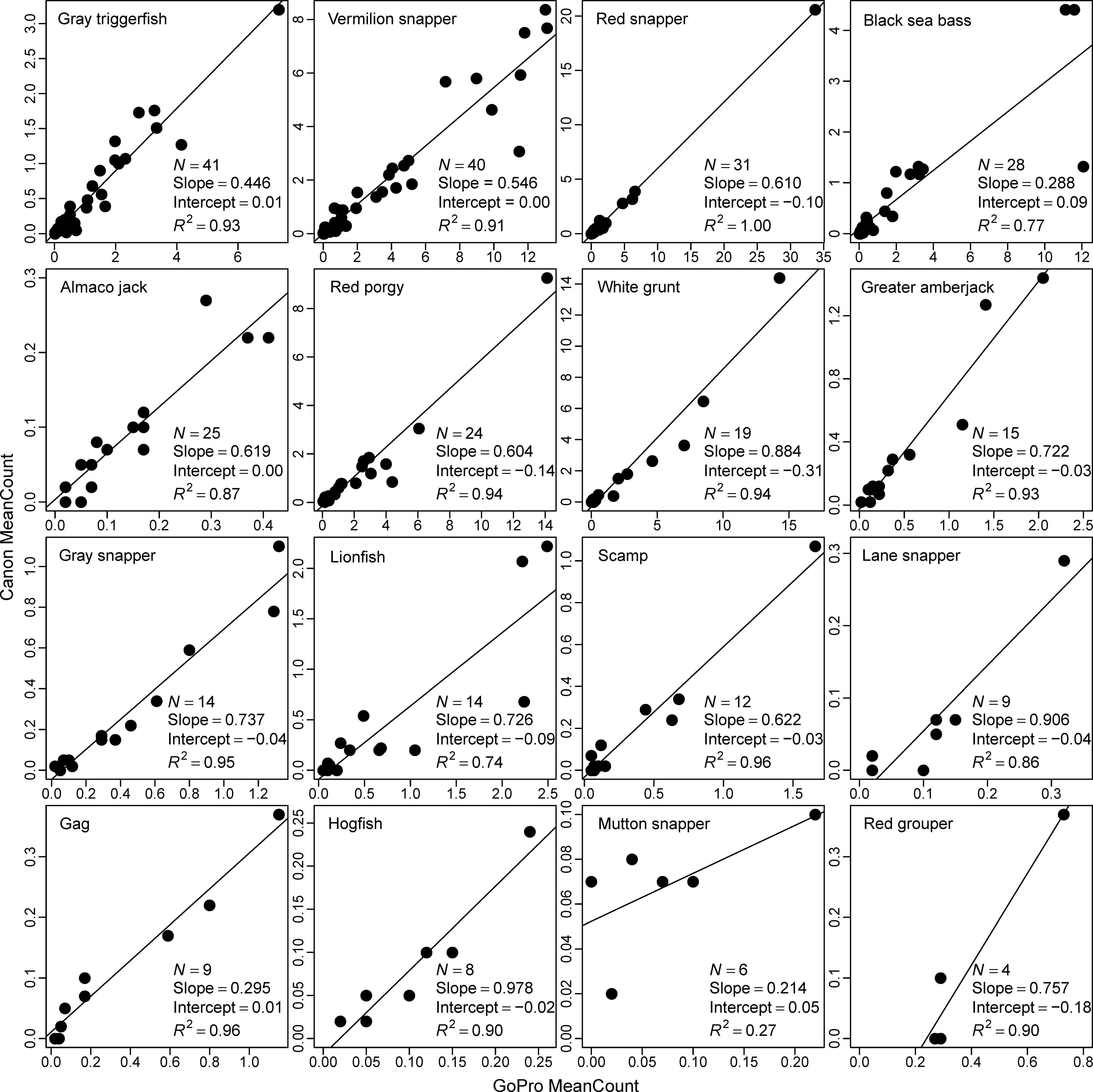
Figure 3 Species-specific calibrations of Canon^® Vixia HF-S200 and GoPro Hero 3+ cameras for 16 reef-associated fish species along the southeast United States Atlantic coast in 2014. Only species observed on at least 4 videos were included here. Slope, intercept, and the R² value were estimated using linear models.

Objective 3: limited sample sizes

The 16 species included in our analyses were represented by 8 families, and these family-level calibrations were generally similar to the species-specific calibrations of members of those families. Five of the eight families only included a single species, so in these cases, the species-level calibrations were identical to the family-level calibrations (i.e., Balistidae, Haemulidae, Labridae, Scorpaenidae, Sparidae; Table 1). The Carangidae family included two species, Lutjanidae included five species, and Serranidae included four species. Family-level slope estimates ranged from 0.293 (Serranidae) to 0.978 (Labridae), with Lutjanidae and Sparidae having slopes most closely resembling the slope of the overall model (Figure 4). Family-level intercepts ranged from -0.31 (Haemulidae) to 0.07 (Serranidae), and the intercept for Lutjanidae (-0.06) again most closely matched the intercept of the overall model (Table 1; Figure 4). The R² values for the family-level calibrations ranged from 0.74 to 0.96, with most being at least 0.90 (Table 1).

FIGURE 4

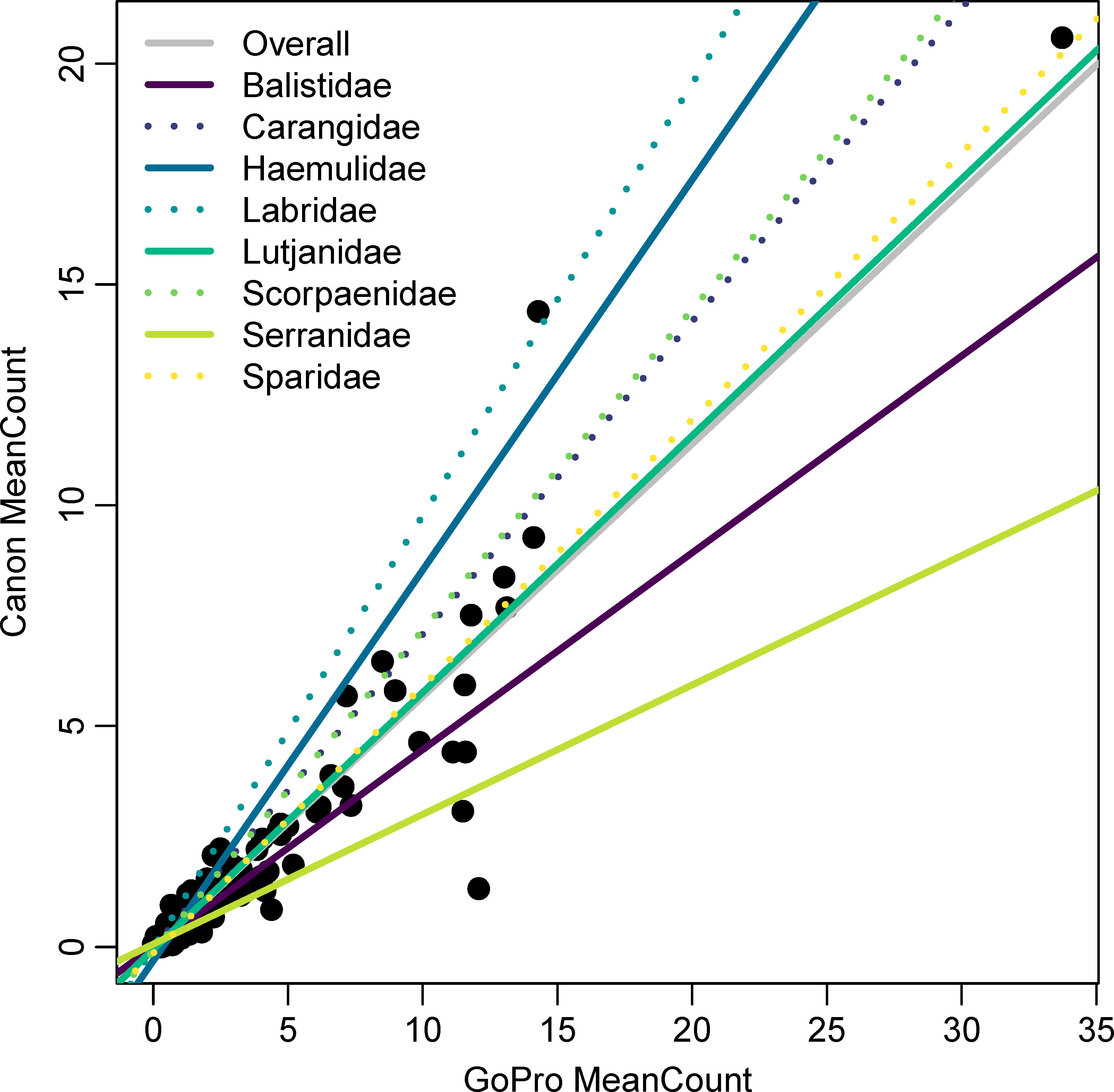
Figure 4 Family-specific calibrations between GoPro Hero 3+ and Canon Vixia HF-S200 cameras from data collected by the Southeast Reef Fish Survey along the southeast United States Atlantic coast in 2014. The overall relationship was estimated using data across all families. Trendlines were estimated using a linear model fit to data across all species within each of the eight families listed.

There were three families that contained more than one species, so calibrations from each of these families were compared to each of the species comprising these families. For Lutjanidae, the two species with the largest sample sizes (i.e., vermilion and red snapper) had calibration slope estimates that were very similar to one another (0.064 difference) and to the family-level calibration (< 0.040; Figure 5). For the remaining lutjanids, as species-specific sample sizes declined, the degree to which their slopes diverged from the family-level calibration increased, with the slope for mutton snapper (N = 4) being most different from Lutjanidae (0.367 difference; Figure 5). For Serranidae, the slope for black sea bass (0.288) and gag Mycteroperca microlepis (0.295) appeared to drive the overall family-level slope (0.293), while the slopes for scamp (0.622) and red grouper (0.757) were very different. Species in the family Carangidae had similar slopes, with the lowest being almaco jack Seriola rivoliana (0.619) and the highest being greater amberjack Seriola dumerili (0.722), with an overall family-level slope of 0.709 (Figure 5).

FIGURE 5

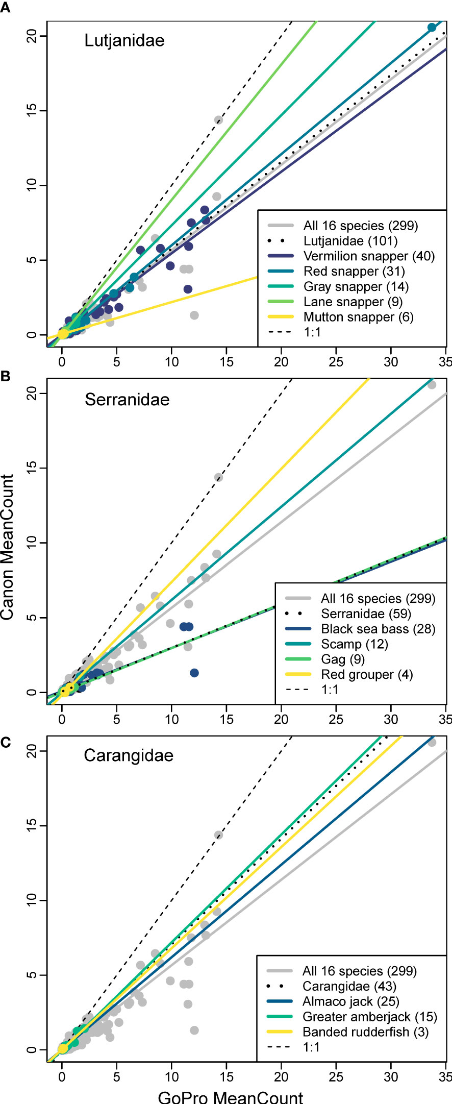
Figure 5 Calibrations between Canon Vixia HF-S200 and GoPro Hero 3+ cameras for various species within three families (A) Lutjanidae; (B) Serranidae; (C) Carangidae from data collected by the Southeast Reef Fish Survey along the southeast United States Atlantic coast in 2014. The overall calibration is shown in gray, family level calibrations are shown by black dotted lines, species’ calibrations are shown by solid colored lines, and the 1:1 relationship is indicated by thin black dashed line. Number in legend indicates sample size for each taxa.

Objective 4: determining optimal approach to apply calibrations

A total of 13,072 videos were included in the scamp and red snapper analyses used to compare two approaches for applying calibrations (Table 2). Sampling was generally consistent across years except for 2020, when no sampling occurred due to the COVID-19 pandemic (Table 2). After model selection, the final scamp negative binomial sub-model included all predictor variables except season, depth, biotic density, and substrate composition, while the scamp binomial sub-model included all variables except current direction. For red snapper, all variables were included in final models except temperature in the negative binomial sub-model and water clarity in the binomial sub-model.

TABLE 2

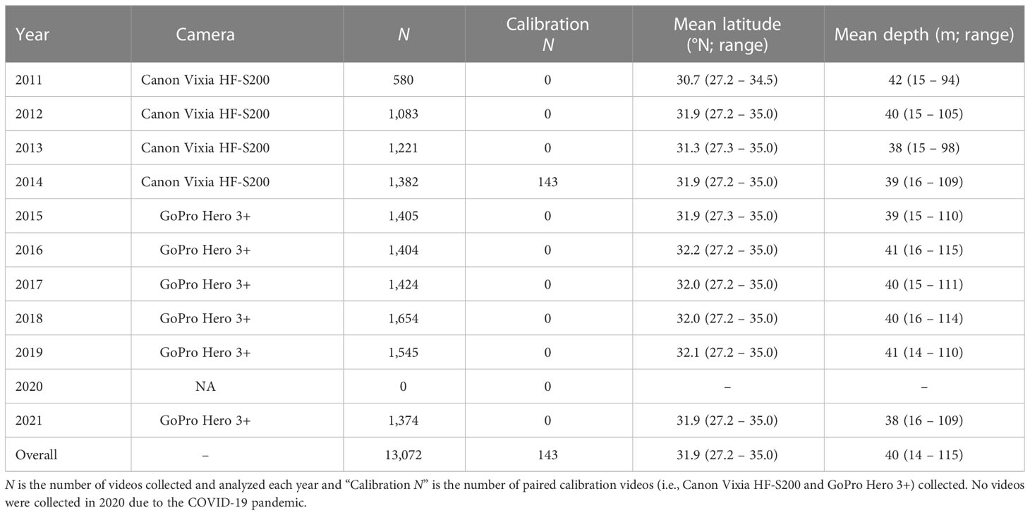
Table 2 Annual video sampling information for the Southeast Reef Fish Survey, 2011–2021, included in the analyses.

Using 2011–2021 video data from SERFS (Table 2), the nominal index of abundance for scamp declined between 2011 and 2013, increased in 2014 and 2015, and declined again from 2015 until 2021 (Figure 6). The standardized index of abundance for scamp completely removed the nominal increase that was evident between 2013 and 2014, instead declining across all years except between 2014 and 2015, when cameras were switched from Canon (2011–2014) to GoPro (2015–2021) in the survey. Calibrating the standardized scamp video index using both approaches removed the increase in relative abundance between 2014 and 2015 entirely, suggesting that increase was due to the increased video counts of scamp on GoPro cameras (relative to Canon cameras) and not an actual increase in abundance. Most importantly, calibrating scamp video data before standardization at the data level, or after standardization at the index level, had very little influence on the resulting scamp index of abundance (Figure 6).

FIGURE 6

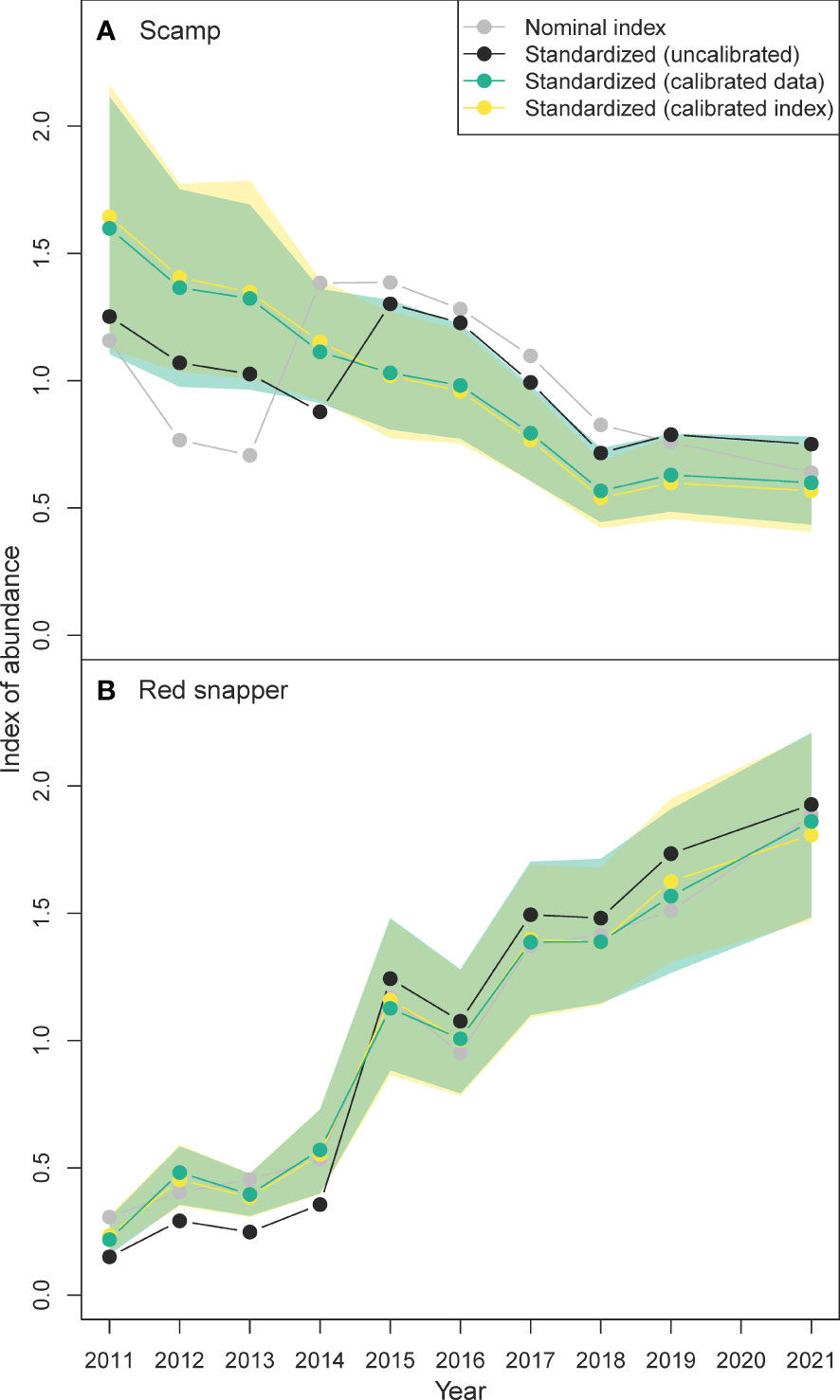
Figure 6 Indices of abundance for (A) scamp Mycteroperca phenax and (B) red snapper Lutjanus campechanus calculated four different ways: (1) a nominal index where no standardization or calibration occurred (gray filled points and line), (2) a standardized index that did not include calibration for a camera switch that occurred between 2014 and 2015 (black filled points and line), (3) a standardized index that included video data that were pre-calibrated before inclusion in a standardization model (blue-green filled points, line, and shaded 95% confidence interval), and (4) a standardized index that was post-calibrated at the index level (yellow filled points, line, and shaded 95% confidence interval). Overlapping 95% confidence intervals are shown in green.

In contrast to scamp, red snapper increased substantially over the course of the study. The nominal red snapper index of abundance increased nearly linearly in all years except between 2015 and 2016, when abundance slightly declined (Figure 6). The standardized index was somewhat different from the nominal index, being lower in 2011–2014 and slightly higher in 2015–2021. Calibration of the standardized index increased abundance in 2011–2014 and decreased abundance in 2015–2021. Consistent with the results for scamp, the standardized red snapper index of abundance was mostly unaffected by which calibration approach was used (Figure 6).

Discussion

Underwater video cameras are widely used to monitor fish abundance and biodiversity (Mallet and Pelletier, 2014), and these cameras have evolved drastically over the last few decades (Struthers et al., 2015). For any video survey, the benefits of utilizing improved technology may at some point outweigh the benefits of maintaining the original gear, yet little to no attention has been given to calibrating video cameras when switches or replacements have occurred. Calibrating different video cameras that are used in fisheries surveys or ecological studies is critical because small differences in camera lenses, sensors, and other characteristics can influence the ability of readers to identify individual fish and therefore affect fish sightability. For instance, a greater field of view of a camera will increase the volume of water sampled, but will also make all objects appear somewhat smaller and thus harder to identify. Therefore, it is critical that researchers carry out empirical calibrations using their cameras, study areas, and target species; theoretical calibrations based on the respective water volume sampled for each camera are unlikely to track closely with empirical calibration results. Video counts are assumed to reflect the true abundance of fish in a way that is not confounded by differing sightabilities of cameras, and this can only be achieved using calibration experiments.

There were substantial differences in fish count calibrations among species from Canon and GoPro cameras. There are likely three main reasons why variability in calibrations was observed among species. The first reason was sample size, whereby species with higher sample sizes had more similar calibrations than species with low sample sizes, whose calibration relationships were much more variable. The second reason was likely due to behavioral variability among species. Some reef fish species are strongly attracted to baited gears, some are indifferent, and some are wary and keep their distance. For example, most species displaying attraction to baited gears (e.g., most lutjanids, carangids, red porgy Pagrus pagrus, gray triggerfish; Bacheler et al., 2022b) had moderate calibration slopes (i.e., 40-50% fewer fish seen on Canon cameras compared to GoPro) because they could be easily viewed by cameras and differences in fields of view between cameras was the primary determinant of the calibration relationships. Black sea bass, on the other hand, were strongly attracted to bait (Bacheler et al., 2013) but highly demersal, leading GoPro cameras with a wider field of view to see individuals close to the camera and on the bottom that Canon cameras could often not see (i.e., 71% fewer individuals observed on Canon cameras). The third reason that may explain some of the variability among species could be differences in their appearance (e.g., size, shape, and color) that might make some species more readily visible and identifiable on some cameras compared to others. For instance, some distinctly shaped fish could be identified far in the background on some cameras compared to nondescript species, which could also influence calibration relationships.

A challenge with video surveys that target multiple species is that calibration factors need to be estimated for all species, but estimating calibrations for rare species can take considerable effort. We evaluated among- and within-family variability in video calibrations to determine if calibrations for related or unrelated species could be used for rare species. Results were species- and family-specific and difficult to generalize. For instance, the behavior of almaco jack, greater amberjack, and banded rudderfish Seriola zonata in family Carangidae is similar (i.e., shoaling, strong curiosity about bait and sampling gears; Campbell et al., 2021), and the resulting calibrations were likewise similar, suggesting that rarely encountered Seriola spp. could justifiably borrow a carangid family-level calibration. That was not the case for species in the family Serranidae, whose calibration slopes were highly variable. Even two species in the same genus of Serranidae like scamp and gag had very different calibration slopes (0.327 difference), suggesting that borrowing calibration information within the family Serranidae is not prudent. These results suggest the safest approach is to collect enough calibration data so that slopes can be estimated well for even the rarest species.

We showed that calibrating video data before standardization or calibrating the index after standardization had a negligible influence on the final index of abundance. This is a particularly encouraging result because it provides researchers flexibility in how to calibrate among video cameras – in some cases it may be easier to calibrate at the data level, whereas in others it is likely much easier to calibrate after index standardization. Note that when calibrating a camera seeing fewer fish to a camera seeing more fish, it is not straightforward to increase the lower camera counts to make them consistent with the higher counts when calibrating at the data level, because it is unclear how to expand when counts are zero on the original camera. To avoid that issue here when calibrating at the data level, we reduced the more recent, higher counts to make them comparable to the earlier, lower counts. In most cases, though, it would probably be preferable to calibrate the previous gear to match the newer gear even if it does not make a difference for a relative index.

Calibration is challenging because sampling gears are often not conducive to being paired in space and time. For instance, trawls are often calibrated by comparing catches from the same general water body in the same season, being pulled near one another at the same time, or being dragged on the same line in succession (Mahon and Smith, 1989; Miller, 2013; Benoit and Cadigan, 2014). Given that fish and environmental conditions are patchily distributed in space and time, often at small scales (Ciannelli et al., 2010; Bacheler et al., 2017), a large amount of residual variation is typically introduced around the estimated calibration factor when gears are not paired in space or time (Pelletier, 1998). Cameras are much more conducive to being paired, given their small size. When calibrating two cameras, we recommend pairing their deployments so that the spatial and temporal variability inherent in fish abundance and environmental conditions can be completely controlled for, and counting fish from the paired samples in exactly the same way (i.e., choosing the same sequential images to analyze). If camera systems are contained in stand-alone metal frames or landers (e.g., Cappo et al., 2004; Merritt et al., 2011; Bacheler and Shertzer, 2015; Amin et al., 2017), it will be necessary to develop a way for these different systems to be paired (i.e., attaching two landers together side-by-side) while not changing the efficiency of each gear compared to when they are deployed independently.

Indices of abundance for scamp and red snapper were improved considerably by accounting for a camera change in 2015 and using a statistical model to standardize video counts among years. Many fishery-independent surveys have used design-based estimators where average catch rates within predetermined sampling strata in a sampling design are calculated, and then an area-weighted sum of abundance in each stratum is produced (Smith, 1990). Due to some downsides of the design-based approach, it has become more common to use statistical models to control for variability in sampling or environmental conditions during the survey (e.g., Helser et al., 2004; Maunder and Punt, 2004; Bacheler and Ballenger, 2018). In our study, nominal (i.e., design-based) indices for scamp and, to a lesser extent, red snapper were different and more variable than standardized indices of abundance (i.e., model-based), the latter of which appeared able to control for environmental variability and changes in the spatial and temporal aspects of sampling among years. Nonetheless, only when the calibration between cameras was accounted for properly did the indices of abundance show smooth declining or increasing trends as expected, highlighting the importance of video calibration studies.

There were some shortcomings of our approach. First, higher calibration sample sizes would have improved calibration relationships, particularly for less commonly observed but important species like red grouper, gag, and hogfish. For instance, red grouper has been observed on 1.4% of videos collected by SERFS in recent years (Bacheler et al., 2019), so approximately 1,429 paired calibration videos would be required to attain an N = 20 for that species. If it is impossible to collect that many calibration videos, we provide a framework for potentially borrowing information from related or unrelated species. A second shortcoming is that we used linear models to relate video counts from one camera to another, when in fact relationships may be nonlinear. In preliminary analyses, we compared linear and nonlinear model fits, which were similar for most species but additional parameters were required for nonlinear models, so linear models were almost always selected by Akaike information criterion (Burnham and Anderson, 2002). Therefore, linear models were used for all comparisons. Third, we selected scamp and red snapper for application of the video calibration (Objective 4), but we cannot conclude that these examples represent all other species. We chose these species for two reasons: (1) indices of abundance were developed for these two species for recent assessments (SEDAR, 2021a; SEDAR, 2021b), and (2) they showed opposite patterns of relative abundance over time, with scamp declining and red snapper increasing, which may have affected calibrations.

Changes in sampling gears can strongly influence the catchability of fish (Arreguín-Sánchez, 1996), leading to biased spatial or temporal trends in relative abundance (Maunder and Punt, 2004). This is especially the case for underwater cameras that are now used widely to provide relative abundance information for various species of fish (Mallet and Pelletier, 2014). Video gears are rapidly evolving, getting smaller and cheaper with higher resolution (Struthers et al., 2015), yet there has been a paucity of examples where calibrations between different video sampling gears occurred. We showed that a camera switch in SERFS in 2015 resulted in much higher fish counts on the new camera compared to the old, which necessitated a calibration experiment to maintain the temporal continuity of the SERFS video survey. We recommend calibrating data from video cameras any time changes occur, and pairing video cameras to the extent possible to control for the spatial and temporal variability inherent in fish populations and environmental conditions. Following these guidelines, researchers will be able to maintain the integrity of valuable long-term video datasets despite changes in their sampling gear that occur out of necessity or by choice.

Data availability statement

The raw data supporting the conclusions of this article will be made available by the authors, without undue reservation.

Ethics statement

The animal study was reviewed and approved by U.S. Government Principles for the Utilization and Care of Vertebrate Animals Used in Testing, Research, and Training.

Author contributions

NB and ZS obtained funding for the calibration experiment, NB, ZS, and LC conceived the research project, ZS coordinated the field data collection, LC, KS, and NB analyzed data, NB and KS drafted the manuscript, and all authors contributed ideas and editorial work on the manuscript. All authors contributed to the article and approved the submitted version.

Funding

This work was funded by the National Marine Fisheries Service.

Acknowledgments

We thank SERFS staff members at the South Carolina Department of Natural Resources and the National Marine Fisheries Service, various volunteers, and the captains and crew of the research vessels for data collection. We also thank R. Cheshire and K. Craig for providing comments on earlier versions of this manuscript.

Conflict of interest

The authors declare that the research was conducted in the absence of any commercial or financial relationships that could be construed as a potential conflict of interest.

Publisher’s note

All claims expressed in this article are solely those of the authors and do not necessarily represent those of their affiliated organizations, or those of the publisher, the editors and the reviewers. Any product that may be evaluated in this article, or claim that may be made by its manufacturer, is not guaranteed or endorsed by the publisher.

Author disclaimer

Mention of trade names or commercial companies is for identification purposes only and does not imply endorsement by the National Marine Fisheries Service, NOAA. The scientific results and conclusions, as well as any views and opinions expressed herein, are those of the authors and do not necessarily reflect those of any government agency.

References

Aguzzi J., Company J. B. (2010). Chronobiology of deep-water decapod crustaceans on continental margins. Adv. Mar. Biol. 58, 155–225. doi: 10.1016/B978-0-12-381015-1.00003-4

PubMed Abstract | CrossRef Full Text | Google Scholar

Amin R., Richards B. L., Misa W. F. X. E., Taylor J. C., Miller D. R., Rollo A. K., et al. (2017). The modular optical underwater survey system. Sensors 17, 2309. doi: 10.3390/s17102309

PubMed Abstract | CrossRef Full Text | Google Scholar

Arreguín-Sánchez F. (1996). Catchability: a key parameter for fish stock assessment. Rev. Fish Biol. Fish. 6, 221–242. doi: 10.1007/BF00182344

CrossRef Full Text | Google Scholar

Bacheler N. M., Ballenger J. C. (2018). Decadal-scale decline of scamp (Mycteroperca phenax) abundance along the southeast united states Atlantic coast. Fish. Res. 204, 74–87. doi: 10.1016/j.fishres.2018.02.006

CrossRef Full Text | Google Scholar

Bacheler N. M., Berrane D. J., Mitchell W. A., Schobernd C. M., Schobernd Z. H., Teer B. Z., et al. (2014). Environmental conditions and habitat characteristics influence trap and video detection probabilities for reef fish species. Mar. Ecol. Prog. Ser. 517, 1–14. doi: 10.3354/meps11094

CrossRef Full Text | Google Scholar

Bacheler N. M., Geraldi N. R., Burton M. L., Muñoz R. C., Kellison G. T. (2017). Comparing relative abundance, lengths, and habitat of temperate reef fishes using simultaneous underwater visual census, video, and trap sampling. Mar. Ecol. Prog. Ser. 574, 141–155. doi: 10.3354/meps12172

CrossRef Full Text | Google Scholar

Bacheler N. M., Gillum Z. D., Gregalis K. C., Pickett E. P., Schobernd C. M., Schobernd Z. H., et al. (2022b). Comparison of video and traps for detecting reef fishes and quantifying species richness in the continental shelf waters of the southeast USA. Mar. Ecol. Prog. Ser. 698, 111–123. doi: 10.3354/meps14141

CrossRef Full Text | Google Scholar

Bacheler N. M., Gillum Z. D., Gregalis K. C., Schobernd C. M., Schobernd Z. H., Teer B. Z. (2020). Spatial patterns in relative abundance and habitat use of adult gray snapper off the southeastern coast of the united states. Mar. Coast. Fish. 12, 205–209. doi: 10.1002/mcf2.10118

CrossRef Full Text | Google Scholar

Bacheler N. M., Runde B. J., Shertzer K. W., Buckel J. A., Rudershausen P. J. (2022a). Fine-scale behavior of red snapper (Lutjanus campechanus) around bait: approach distances, bait plume dynamics, and effective fishing area. Can. J. Fish. Aquat. Sci. 79, 458–471. doi: 10.1139/cjfas-2021-0044

CrossRef Full Text | Google Scholar

Bacheler N. M., Schobernd Z. H., Berrane D. J., Schobernd C. M., Mitchell W. A., Geraldi N. R. (2013). When a trap is not a trap: converging entry and exit rates and their effect on trap saturation of black sea bass (Centropristis striata). ICES J. Mar. Sci. 70, 873–882. doi: 10.1093/icesjms/fst062

CrossRef Full Text | Google Scholar

Bacheler N. M., Schobernd Z. H., Gregalis K. C., Schobernd C. M., Teer B. Z., Gillum Z., et al. (2019). Patterns in fish biodiversity associated with temperate reefs on the southeastern US continental shelf. Mar. Biodiv. 49, 2411–2428. doi: 10.1007/s12526-019-00981-9

CrossRef Full Text | Google Scholar

Bacheler N. M., Shertzer K. W. (2015). Estimating relative abundance and species richness from video surveys of reef fishes. Fish. Bull. 113, 15–26. doi: 10.7755/FB.113.1.2

CrossRef Full Text | Google Scholar

Bacheler N. M., Shertzer K. W. (2020). Catchability of reef fish species in traps is strongly affected by water temperature and substrate. Mar. Ecol. Prog. Ser. 642, 179–190. doi: 10.3354/meps13337

CrossRef Full Text | Google Scholar

Balletti C., Guerra F., Tsioukas V., Vernier P. (2014). Calibration of action cameras for photogrammetric purposes. Sensors 14, 17471–17490. doi: 10.3390/s140917471

PubMed Abstract | CrossRef Full Text | Google Scholar

Benoit H. P., Cadigan N. (2014). Model-based estimation of commercial-sized snow crab (Chionoecetes opilio) abundance in the southern gulf of st. Lawrence 1980-2013, using data from two bottom trawl surveys. DFO Can. Sci. Advis. Sec. Res. Doc.

Google Scholar

Brooks E. J., Sloman K. A., Sims D. W., Danylchuk A. J. (2011). Validating the use of baited remote underwater video surveys for assessing the diversity, distribution and abundance of sharks in the Bahamas. Endanger. Species Res. 13, 231–243. doi: 10.3354/esr00331

CrossRef Full Text | Google Scholar

Burnham K. P., Anderson D. R. (2002). Model selection and multimodal inference: a practical information-theoretic approach. 2nd edn (New York: Springer).

Google Scholar

Cadigan N. G., Dowden J. J. (2010). Statistical inference about the relative efficiency of a new survey protocol, based on paired-tow survey calibration data. Fish. Bull. 108, 15–30.

Google Scholar

Campbell M. D., Huddleston A., Somerton D., Clarke M. E., Wakefield W., Murawski S., et al. (2021). Assessment of attraction and avoidance behaviors of fish in response to the proximity of transiting underwater vehicles. Fish. Bull. 119, 216–230. doi: 10.7755/FB.119.4.2

CrossRef Full Text | Google Scholar

Campbell M. D., Salisbury J., Caillouet R., Driggers W. B., Kilfoil J. (2018). Camera field-of-view and fish abundance estimation: a comparison of individual-based model output and empirical data. J. Exp. Mar. Biol. Ecol. 501, 46–53. doi: 10.1016/j.jembe.2018.01.004

CrossRef Full Text | Google Scholar

Cappo M., Speare P., Ge’ath G. (2004). Comparison of baited remote underwater video stations (BRUVS) and prawn (shrimp) trawls for assessments of fish biodiversity in inter-reefal areas of the great barrier reef marine park. J. Exp. Mar. Biol. Ecol. 302, 123–152. doi: 10.1016/j.jembe.2003.10.006

CrossRef Full Text | Google Scholar

Ciannelli L., Knutsen H., Olsen E. M., Espeland S. H., Asplin L., Jelmert A., et al. (2010). Small-scale genetic structure in a marine population in relation to water circulation and egg characteristics. Ecol. 91, 2918–2930. doi: 10.1890/09-1548.1

CrossRef Full Text | Google Scholar

Dennis D., Plagányi É., Van Putten I., Hutton T., Pascoe S. (2015). Cost benefit of fishery-independent surveys: are they worth the money? Mar. Pol. 58, 108–115. doi: 10.1016/j.marpol.2015.04.016

CrossRef Full Text | Google Scholar

Dorman S. R., Harvey E. S., Newman S. J. (2012). Bait effects in sampling coral reef fish assemblages with stereo-BRUVs. PloS One 7 (7), e41538. doi: 10.1371/journal.pone.0041538

PubMed Abstract | CrossRef Full Text | Google Scholar

Ellis D. M., DeMartini E. E. (1995). Evaluation of a video camera technique for indexing the abundances of juvenile pink snapper, Pristipomoides filamentosus, and other Hawaiian insular shelf fishes. Fish. Bull. 93, 67–77.

Google Scholar

Goethel D. R., Omori K. L., Punt A. E., Lynch P. D., Berger A. M., de Moor C. L., et al. (2022). Oceans of plenty? challenges, advancements, and future directions for the provision of evidence-based fisheries management advice. Rev. Fish Biol. Fish. doi: 10.1007/s11160-022-09726-7

CrossRef Full Text | Google Scholar

Hamner R. M., Freshwater D. W., Whitfield P. E. (2007). Mitochondrial cytochrome b analysis reveals two invasive lionfish species with strong founder effects in the western Atlantic. J. Fish Biol. 71, 214–222. doi: 10.1111/j.1095-8649.2007.01575.x

CrossRef Full Text | Google Scholar

Hangsleben M. A., Allen M. S., Gwinn D. C. (2013). Evaluation of electrofishing catch per unit effort for indexing fish abundance in Florida lakes. Trans. Am. Fish. Soc 142, 247–256. doi: 10.1080/00028487.2012.730106

CrossRef Full Text | Google Scholar

Harvey E. S., Cappo M., Butler J. J., Hall N., Kendrick G. A. (2007). Bait attraction affects the performance of remote underwater video stations in assessment of demersal fish community structure. Mar. Ecol. Prog. Ser. 350, 245–254. doi: 10.3354/meps07192

CrossRef Full Text | Google Scholar

Harvey E. S., Shortis M. (1998). Calibration stability of an underwater stereo-video system: implications for measurement accuracy and precision. Mar. Technol. Soc J. 329, 3–17.

Google Scholar

Heagney E. C., Lynch T. P., Babcock R. C., Suthers I. M. (2007). Pelagic fish assemblages assessed using mid-water baited video: standardizing fish counts using bait plume size. Mar. Ecol. Prog. Ser. 350, 255–266. doi: 10.3354/meps07193

CrossRef Full Text | Google Scholar

Helser T. E., Punt A. E., Methot R. D. (2004). A generalized linear mixed model analysis of a multi-vessel fishery resource survey. Fish. Res. 70, 251–264. doi: 10.1016/j.fishres.2004.08.007

CrossRef Full Text | Google Scholar

Kimura D. K., Somerton D. A. (2006). Review of statistical aspects of survey sampling for marine fisheries. Rev. Fish. Sci. 14, 245–283. doi: 10.1080/10641260600621761

CrossRef Full Text | Google Scholar

Kumpf H. E., Lowenstein J. M. (1962). Undersea observation station. Sea Front. 8, 198–206.

Google Scholar

Letessier T. B., Juhel J. B., Vigliola L., Meeuwig J. J. (2015). Low-cost small action cameras in stereo generates accurate underwater measurements of fish. J. Exp. Mar. Biol. Ecol. 466, 120–126. doi: 10.1016/j.jembe.2015.02.013

CrossRef Full Text | Google Scholar

Mahon R., Smith R. W. (1989). Comparison of species composition in a bottom trawl calibration experiment. J. Northw. Atl. Fish. Sci. 9, 73–79. doi: 10.2960/J.v9.a6

CrossRef Full Text | Google Scholar

Mallet D., Pelletier D. (2014). Underwater video techniques for observing coastal marine biodiversity: a review of sixty years of publications, (1952–2012). Fish. Res. 154, 44–62. doi: 10.1016/j.fishres.2014.01.019

CrossRef Full Text | Google Scholar

Maunder M. N., Piner K. R. (2015). Contemporary fisheries stock assessment: many issues still remain. ICES J. Mar. Sci. 72, 7–18. doi: 10.1093/icesjms/fsu015

CrossRef Full Text | Google Scholar

Maunder M. N., Punt A. E. (2004). Standardizing catch and effort data: a review of recent approaches. Fish. Res. 70, 141–159. doi: 10.1016/j.fishres.2004.08.002

CrossRef Full Text | Google Scholar

Merritt D., Donovan M. K., Kelley C., Waterhouse L., Parke M., Wong K., et al. (2011). BotCam: a baited camera system for nonextractive monitoring of bottomfish species. Fish. Bull. 109, 56–67.

Google Scholar

Miller T. J. (2013). A comparison of hierarchical models for relative catch efficiency based on paired-gear data for US Northwest Atlantic fish stocks. Can. J. Fish. Aquat. Sci. 70, 1306–1316. doi: 10.1139/cjfas-2013-0136

CrossRef Full Text | Google Scholar

Murphy H. M., Jenkins G. P. (2010). Observational methods used in marine spatial monitoring of fishes and associated habitats: a review. Mar. Freshw. Res. 61, 236–252. doi: 10.1071/MF09068

CrossRef Full Text | Google Scholar

Myrberg A. A., Banner A., Richard J. D. (1969). Shark attraction using a video-acoustic system. Mar. Biol. 2, 264–276. doi: 10.1007/BF00351149

CrossRef Full Text | Google Scholar

Pelletier D. (1998). Intercalibration of research survey vessels in fisheries: a review and an application. Can. J. Fish. Aquat. Sci. 55, 2672–2690. doi: 10.1139/f98-151

CrossRef Full Text | Google Scholar

Priede I. G., Merrett N. R. (1996). Estimating of abundance of abyssal demersal fishes: a comparison of data from trawls and baited cameras. J. Fish Biol. 49 (Suppl A), 207–216. doi: 10.1111/j.1095-8649.1996.tb06077.x

CrossRef Full Text | Google Scholar

R Core Team (2021). R: a language and environment for statistical computing (Vienna, Austria: R Foundation for Statistical Computing). Available at: https://www.R-project.org/.

Google Scholar

Santana-Garcon J., Braccini M., Langlois T. J., Newman S. J., McAuley R. B., Harvey E. S. (2014). Calibration of pelagic stereo-BRUVs and scientific longline surveys for sampling sharks. Meth. Ecol. Evol. 5, 824–833. doi: 10.1111/2041-210X.12216

CrossRef Full Text | Google Scholar

Schobernd Z. H., Bacheler N. M., Conn P. B. (2014). Examining the utility of alternative video monitoring metrics for indexing reef fish abundance. Can. J. Fish. Aquat. Sci. 71, 464–471. doi: 10.1139/cjfas-2013-0086

CrossRef Full Text | Google Scholar

SEDAR (2021a) SEDAR 73 stock assessment report: south Atlantic red snapper. Available at: https://sedarweb.org/documents/sedar-73-stock-assessment-report-south-atlantic-red-snapper/.

Google Scholar

SEDAR (2021b) SEDAR 68 stock assessment report: Atlantic scamp grouper. Available at: https://sedarweb.org/documents/sedar-68-atlantic-scamp-final-stock-assessment-report/.

Google Scholar

Shafait F., Harvey E. S., Shortis M. R., Mian A., Ravanbakhsh M., Seager J. W., et al. (2017). Towards automating underwater measurement of fish length: a comparison of semi-automatic and manual stereo-video measurements. ICES J. Mar. Sci. 74, 1690–1701. doi: 10.1093/icesjms/fsx007

CrossRef Full Text | Google Scholar

Smith S. J. (1990). Use of statistical models for the estimation of abundance from groundfish trawl survey data. Can. J. Fish. Aquat. Sci. 47, 894–903. doi: 10.1139/f90-103

CrossRef Full Text | Google Scholar

Struthers D. P., Danylchuk A. J., Wilson A. D. M., Cooke S. J. (2015). Action cameras: bringing aquatic and fisheries research into view. Fisheries 40, 502–512. doi: 10.1080/03632415.2015.1082472

CrossRef Full Text | Google Scholar

Thorson J. T., Ward E. J. (2014). Accounting for vessel effects when standardizing catch rates from cooperative surveys. Fish. Res. 155, 168–176. doi: 10.1016/j.fishres.2014.02.036

CrossRef Full Text | Google Scholar

Tyre A. J., Tenhumberg B., Field S. A., Niejalke D., Parris K., Possingham H. P. (2003). Improving precision and reducing bias in biological surveys: estimating false-negative error rates. Ecol. Appl. 13, 1790–1801. doi: 10.1890/02-5078

CrossRef Full Text | Google Scholar

Whitmarsh S. K., Fairweather P. G., Huveneers C. (2017). What is big BRUVver up to? methods and uses of baited underwater video. Rev. Fish Biol. Fish. 27, 53–73. doi: 10.1007/s11160-016-9450-1

CrossRef Full Text | Google Scholar

Zeileis A., Kleiber C. (2017). “Countreg: count data regression,” in R package version0.0/r34.

Google Scholar

Zeileis A., Kleiber C., Jackman S. (2008). Regression models for count data in r. J. Stat. Software 27, 1–25. doi: 10.18637/jss.v027.i08

CrossRef Full Text | Google Scholar

Zuur A. F., Ieno E. N., Walkder N. J., Saveliev A. A., Smith G. M. (2009). Mixed effects models and extensions in ecology with r (New York: Spring Science and Business Media, LLC).

Google Scholar