 Veronica Frassà1*
 Aristides M. Prospathopoulos2
 Alessio Maglio3
 Noelia Ortega4Romulus-Marian Paiu5,6
 Arianna Azzellino1
- 1Department of Civil and Environmental Engineering (DICA), Politecnico di Milano, Milano, Italy
- 2Hellenic Centre for Marine Research (HCMR), Institute of Oceanography, Anavyssos, Greece
- 3SINAY Maritime Data Solution, Caen, France
- 4Centro Tecnológico Naval y del Mar, Centro Tecnologico Naval (CTN)-Marine Technology Centre, Parque Tecnológico de Fuente Álamo, Fuente Alamo, Spain
- 5Mare Nostrum Non-governmental Organization (NGO), Constanța, Romania
- 6Biology Faculty, Bucharest University, Bucharest, Romania
Sighting data deriving from the ACCOBAMS1 Survey Initiative (ASI), conducted through the CeNoBS2 project, enabled the investigation of the habitat preferences for three different cetacean subspecies occurring in the Black Sea waters: the bottlenose dolphins (Tursiops truncatus), the common dolphins (Delphinus delphis) and the harbour porpoise (Phocoena phocoena). ASI aerial surveys, aiming at assessing the distribution and abundance of cetacean populations, were conducted during summer of 2019 in waters in front of Romania, Georgia, Bulgaria, Turkey and Ukraine. The surveys allowed recording of 1716 sightings: 117 bottlenose dolphins, 715 common dolphins and 884 harbour porpoises. The aim of this study was twofold: (i) to develop habitat models, using physical characteristics, such as depth and slope, as covariates, in order to estimate the presence probability of the three cetacean species in the Black Sea; (ii) to demonstrate the usefulness of the habitat models in support of environmental status assessments on marine mammals where the stressor is the shipping noise. The results of this study show the reliability of physical covariates as predictors of the probability of occurrence for the three species of interest in the Black Sea, providing additional knowledge, complementary to abundance estimates, which may support the assessment of the vulnerability of marine areas to different pressures, including noise.
1 Introduction
The Black Sea is a naturally isolated body of water with a unique marine environment. Three subspecies of cetaceans can be found in there: the Black Sea bottlenose dolphin (Tursiops truncatus ponticus) (Barabash-Nikiforov, 1940), the Black Sea common dolphin (Delphinus delphis ponticus) (Barabash, 1935), and the Black Sea harbour porpoise (Phocoena phocoena relicta) (Abel, 1905). For many years it was legal to catch cetaceans in the Black Sea during commercial fishing (Smith, 1982; Birkun, 2002), causing a decline in the populations of these three cetacean species (Smith, 1982; Zemsky, 1994; Sánchez-Cabanes et al., 2017; BSC, 2008; Tonay and Öztürk, 2012). It was only in 1966 that such activities were banned in the Russian Federation, Bulgaria and Romania, and in 1983 in Turkey (Smith, 1982; Tonay and Öztürk, 2012; Sánchez-Cabanes et al., 2017). Despite these bans, incidental and illegal catches continue to be present and documented (Buckland et al., 1992; Birkun, 2002; Gol’din and Gol’din, 2004). Due to the historical situation outlined above, both the Black Sea bottlenose dolphin and harbour porpoise have been classified as endangered species, while the Black Sea common dolphin is listed as vulnerable on the IUCN Red List of Threatened Species (Birkun and Frantzis, 2008; Birkun, 2012; IUCN, 2012; ACCOBAMS, 2021b; ACCOBAMS, 2023). Besides the incidental catches, the considered species are subject to other major anthropogenic pressures such as collisions, underwater noise and chemical pollution (IUCN, 2012).
Monitoring surveys in the Black Sea have been limited, with most large-scale surveys conducted prior to 1987. Recent efforts have focused on local surveys in coastal areas (Birkun et al., 2004, Birkun et al., 2004; Dede and Tonay, 2010; Birkun et al., 2014 Kopaliani et al., 2015; Panayotova and Todorova, 2015; Gladilina and Gol’din, 2016; Gladilina et al., 2017; Popov et al., 2017; Baș et al., 2019; Paiu et al., 2019).
Collaborative aerial surveys have also been undertaken to gather valuable information about these species (Birkun et al., 2004; Raykov and Panayotova, 2012; Radu et al., 2013; Sánchez-Cabanes et al., 2017). However, prior to the CeNoBS initiative (ACCOBAMS 2021a), a comprehensive assessment of the overall abundance and distribution of these cetacean species in the Black Sea was not available. CeNoBS, with its systematic and synoptic approach, has provided a significant advancement in our understanding of the abundance, distribution, and density of all three cetacean species in the Black Sea during the summer months.
In the European Strategy for Marine and Maritime Research (COM (2008) 534), it is highlighted how important it is to reconcile environmental sustainability with the growth of maritime activities in order to decrease their strong environmental impact. Marine mammals are recognized by the EU Marine Strategy Framework Directive, as flagship species and therefore an essential element of ecosystem sustainability (Hooker and Gerber, 2014), their protection being a priority issue, requiring a robust analysis of existing information and data to identify areas requiring priority conservation actions (Pennino et al., 2013a; Pennino et al., 2016). Modelling the habitat of marine mammal may offer a fundamental understanding of the ecological processes that determine the population distributions (Redfern et al., 2006; Embling et al., 2010), allowing a better understanding of the ecology of these animals (Sánchez-Cabanes et al., 2017; Hamazaky, 2002) and providing a tool which can support management (Azzellino et al., 2012; Forney et al., 2012; Mannocci et al., 2014; Cribb et al., 2015; Pennino et al., 2017).
As part of the QUIETSEAS project (www.quietseas.eu), a methodological framework was created specifically for the Mediterranean Sea and Black Sea (Azzellino et al., 2023, Deliverable 5.2) and continuous noise, aligning with the guidelines provided by the TG Noise (EU Technical Group on Underwater Noise for providing guidance to the Member States on the implementation of the Marine Strategy Framework Directive (MSFD) as regards Descriptor 11 (Energy including Underwater Noise) of the Directive). This framework enables the quantification of the impact of continuous noise sources on the potential habitat of the primary cetacean species in the Mediterranean Sea and Black Sea. The methodology introduced in this project utilizes habitat models, which make it possible to estimate the likelihood of species presence by considering bathymetric characteristics. Additionally, acoustic propagation models are employed to analyse the noise sources under consideration. By integrating these components, the framework facilitates the assessment of the reduction in potential cetacean habitat caused by noise. Regarding the habitat models, preference was given to models incorporating physical covariates, as they have been widely employed in ecological studies (Frankel et al., 1995; Gowans and Whitehead, 1995; Baumgartner, 1997; Raum-Suryan and Harvey, 1998; Karczmarski et al., 2000; Ferguson and Barlow, 2001; Ferguson et al., 2006a; Ferguson et al., 2006b; Azzellino et al., 2008; Azzellino et al., 2012; Blasi and Boitani, 2012; Marini et al., 2015) and offer greater stability and applicability across various study areas. This choice is based on their proven track record and reliability. In contrast, dynamic predictors like chlorophyll-a or surface sea temperature, exhibit considerable temporal and spatial variations due to factors such as seasonal fluctuations, interannual variability, and localized dynamics.
However, while habitat models based on physical predictors, and built upon a robust, long-term observation time series (Azzellino et al., 2012) have been available for the Mediterranean Sea, a comparable model specific to the Black Sea has not been readily accessible.
The primary objective of this study is to develop presence/absence habitat models for the cetacean species in the Black Sea, utilizing large-scale survey data and employing habitat physical characteristics as predictors.
This endeavour aims to expand the current QUIETSEAS methodological framework, which assesses the impact of continuous noise, to encompass the Black Sea region. By doing so, we aim to enhance our understanding of the effects of continuous noise on the marine environment in the Black Sea and its implications for cetacean species, supporting the implementation of the Marine Strategy Framework Directive (MFSD) and other relevant legal frameworks.
2 Material and methods
2.1 Study area
The Black Sea is a semi-closed basin covering an area of 436400 km2 and constituting a unique marine environment, with a maximum depth of 2200 m (Murray et al., 1989). The Black Sea is connected by the Kerch Strait to the smallest and shallowest sea in the world (14 m maximum), called the Sea of Azov, located in the north-eastern part of the basin. Through the Istanbul Strait (Bosphorus), it is connected to the Sea of Marmara, which in turn is connected to the Aegean Sea through the Çanakkale Strait (Dardanelles) (Özsoy and Ünlüata, 1997). The continental shelf, at depths < 200 m, constitutes about 25% of the total area, while the flat abyssal plain, at depths > 2000 m, occupies about 60% of the total area. There are many steep slopes adjacent to the mainland and submarine canyons, such as Sakarya Canyon, in the southwestern area, where the depth suddenly increases from 100 m to 1500 m (Murray et al., 1989). It is important to mention that Black Sea has a positive water balance, where inputs from freshwater sources exceed evaporation losses. The freshwater inflow has great seasonal and inter-annual variability, having the Danube, Dnepr and Dnestr as the main rivers flowing into the North-West shelf (Murray et al., 1989). The water layer above 200 m is well oxygenated, while the deeper layer (between 200 and 2200 m) is anoxic. About 87% of the Black Sea water mass is therefore anoxic and contains high levels of sulphide, making pelagic and benthic organisms largely absent (Sánchez-Cabanes et al., 2017). The Black Sea is also characterized by low salinity levels due to high freshwater outflow from rivers and inflow from the Mediterranean with higher salinity and density, thus creating high water stratification. The temperature has a seasonal and regional variation, with an average annual surface temperature ranging between 16°C in the south and 11°C in the northwest (Balkas et al., 1990; Sánchez-Cabanes et al., 2017). The Black Sea hosts a wide variety of habitats, but relatively low biodiversity resulting in the absence of many local competitors, generating favourable conditions for invasive species which pose a great threat to the biodiversity of the Black Sea (Oğuz and Öztürk, 2011; Selifonova, 2011). The anoxic conditions and strong contrast in temperature and salinity make the ecology of the Black Sea vulnerable to anthropogenic effects compared to the Mediterranean and open seas (Kideys, 2002; Sánchez-Cabanes et al., 2017). The three cetacean subspecies that can be found regularly (Black Sea bottlenose dolphins, Black Sea common dolphins and Black Sea harbour porpoises) are distinct subspecies from the Mediterranean and Atlantic populations and are endemic to the Black Sea and the Sea of Azov (Birkun, 2002). The three species are at the top of the trophic network of the basin and have no natural predators (Kleinenberg, 1956; Jefferson et al., 2008).
2.2 Data set and data collection
The data used for this study were collected through the EU-funded CeNoBS project, in collaboration with and co-funded by ACCOBAMS under the ACCOBAMS Survey Initiative (ASI). The CeNoBS project (ACCOBAMS, 2021a; Paiu et al., 2021) supported the implementation of the MSFD in the Black Sea through the establishment of a regional cetacean monitoring system and noise monitoring to assess the status of cetaceans in the Black Sea through MSFD descriptors and particularly of Descriptors 1 (D1, Biological Diversity) and Descriptor D11 (Energy including Underwater Noise).
CeNoBS data were collected through regional aerial surveys conducted in the Black Sea between June and July 2019, following specific shared protocols. Data were collected, following the distance sampling method (Buckland et al., 2015), by observers on board small twin-engine aircrafts, equipped with bubble windows, allowing the sight of cetaceans and other marine megafauna below the aircraft. Specific transects were designed and prepared to ensure fair coverage and representation of the study area. The surveys covered the waters in front of Romania, Bulgaria, Turkey, Ukraine and Georgia. The transects were predefined and adapted to the flight limitations in some areas. Six blocks and zigzag traces were drawn for each of them in order to have a minimum coverage of 3% of the study areas (Paiu et al., 2021) (Figure 1). Two observers, a team leader and the pilot were on board. Data were collected according to specific protocols prepared by the project’s researchers and scientific collaborators. During the surveys, target altitude was 183 m (600 feet) with target speed of 100 knots. The software used to collect data was SAMMOA dedicated to marine megafauna data collection (SAMMOA 1.1.2, 2017-2018; Pelagis Observatory-La Rochelle University-CNRS), linked to GPS to collect position data (Paiu et al., 2021). Data regarding environmental conditions were collected at the beginning of each transect and whenever a change occurred. Variables considered were sea state (Beaufort scale), glare, cloud cover and sighting conditions. The three cetacean species (common dolphin, bottlenose dolphin and harbour porpoise) were the main target species, and data were collected also on group size and composition [mixed groups and two age classes Adults and Juveniles (calves)], swimming direction and group behaviour (using 8 defined categories) (SCANS II, 2008; Hammond et al., 2013).
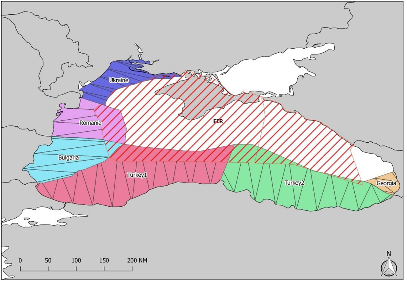
Figure 1 The six blocks and tracks covered by planes in the waters of Romania, Bulgaria, Turkey, Ukraine and Georgia (map source: ACCOBAMS-CeNoBS project).
The survey was conducted flying along the planned surveys primarily in passive mode, unless it was necessary to confirm species, obtain reliable estimates of school size, composition or behaviour by circling over the sighted animals. The survey was then resumed at the exact point it was left and all the secondary sightings (i.e. the additional sightings made after leaving the predetermined trackline) although recorded have not been used to obtain the abundance and density estimates.
CeNoBS aerial surveys were carried out from 17 June 2019 to 4 July 2019. A total of 15246 km of effort were surveyed: 9354 km on-effort and 5892 km off-effort. A total of 1984 sightings were collected, belonging to the three target species regularly occurring in the Black Sea. Sightings were distributed as follows: Bottlenose dolphins: 117 sightings and 335 individuals; Common dolphin: 715 sightings and 1762 individuals; Harbour porpoises 884 sightings and 1522 individuals; Delphinidae (unidentified species when a common dolphin or bottlenose dolphin was involved, mostly was due to size of the animal (juvenile) or poor sightability conditions such as relfexion, glare, swell etc): 28 sightings and 50 individuals (Paiu et al., 2021). Figure 2 shows the sighting distribution in the study area.
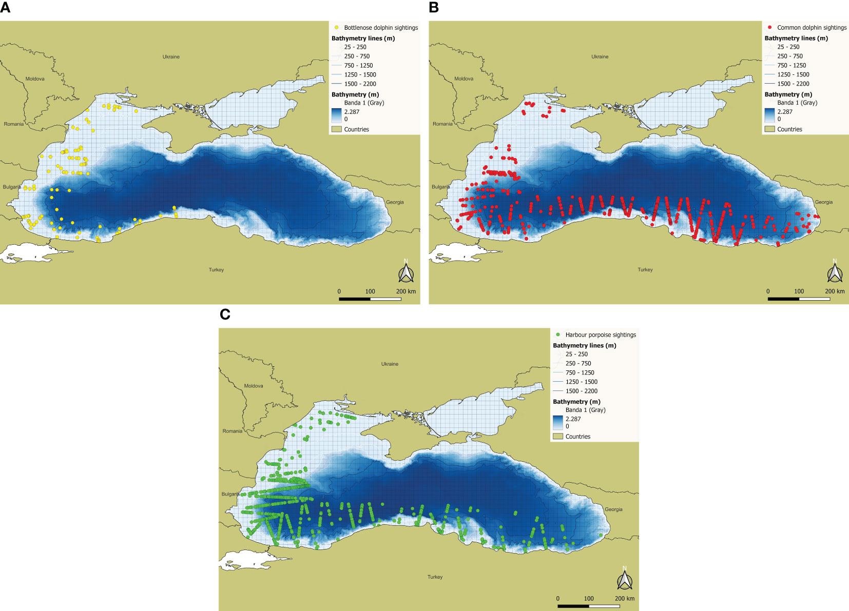
Figure 2 CeNoBS sightings: (A) Bottlenose dolphin; (B) Common dolphin; (C) Harbour porpoise.
2.3 Data analysis
2.3.1 Data matrix preparation
Using QGIS 3.20.3, a grid was created for the Black Sea with a total of 2069 cells of size 0.16° x 0.16° (10 nm x 10 nm, corresponding to 18.5 km x 18.5 km). Bathymetric data were obtained through GEBCO with a 2021 model, providing elevation data in metres on a grid at 15 arc second intervals (https://download.gebco.net/). Sea bed slope was calculated using QGIS 3.20.3 from the depth layer via the GDAL slope command. Bathymetric data were integrated with the grid, enabling the calculation of depth and slope statistics within each cell. Such statistics were later used as potential covariates for the habitat models. The statistics calculated were mean, median, minimum value, maximum value, standard deviation and range (in metres for depth and in percentage value for slope). Moreover, the searching effort (i.e. length of track line in kilometres), and the sightings of each species were associated with the grid cells, and integrated with the data matrix needed for the following analysis.
2.3.2 Habitat model development
Habitat model development and evaluation was conducted by means of a binary logistic regression analysis, used also in similar ecological applications (Guisan and Zimmermann, 2000; Davis et al., 2002; Azzellino et al., 2008; Anderwald et al., 2011; Azzellino et al., 2011). All the analyses were performed using the IBM SPSS Statistics package (version 27). To make the analysis more efficient, the number of absence cells (i.e. pseudo-absence of the target species) in the dataset was balanced with the number of presence cells (presence of 1 or more sightings of the target species). Following Azzellino et al. (2012), the total number of presence cells was in fact maintained, while a number of absence cells (absence of sightings) equal to the number of presence cells was randomly extracted from the overall number of absence cells. Moreover, the binary logistic regression was applied using a stepwise approach, based on Wald statistics (Hosmer and Lemeshow, 2000) in order to select the best set of predictors. Each predictor was tested for entry into the model one by one, based on the significance level of the Wald statistic. After each entry, variables already in the model were tested again for possible removal. The procedure stopped when no more variables met the entry or removal criteria or when the last fitted model was the same as the previous. To prevent the risk of overfitting, each specific model was limited to a maximum of three predictors ensuring a sufficient number of observations, exceeding ten for each predictor. Additionally, the model’s accuracy in terms of classification performance was assessed using leave-one-out cross-validation.
2.3.3 Noise magnitude assessment
The noise assessment was conducted following the risk-based methodological approach drafted in Deliverable 3 of the EU TG Noise (TG Noise, 2021). Following the risk-based approach, the probability of having an effect on a population exposed to a given pressure (i.e. continuous noise) can be estimated by considering the magnitude of the pressure (i.e. the noise level) and the effective exposure which depends on the presence of vulnerable species within the study area.
Based on TG Noise framework, the starting point of the methodology is the selection of habitats of the target species, at regional or subregional or at the Marine Reporting Unit (MRU) level. Afterwards, the habitat status is assessed within a reference grid where the condition in each grid cell is evaluated referring to the current state or to a reference condition. The deviation of the current state from the reference condition enables to evaluate whether the cell is non-significantly or significantly affected by the anthropogenic noise (Annex 7-TG Noise – Sigray et al., 2021). All the grid cells of the habitat will thus be quantified both in time and space as significantly or non-significantly affected. Thus, for a specific time period, a certain fraction of the grid cells will be significantly affected. The potential for adverse effects at population level is assumed to occur when a certain fraction of the habitat is exposed to continuous noise for a certain fraction of time. Area and duration of exposure to anthropogenic sound can be assessed in terms of:
- Tolerable impacted area of the habitat
- Tolerable duration of the noise.
More specifically, based on the TG Noise methodological framework, the noise exposure and the consequent potential impact on the species of interest needs to be assessed following different methodological steps. As a first step a noise exposure map for the study area was generated covering the period from 01.07.2018 to 31.08.2018 using a reference grid of 100 m x 100 m mesh size. Three daily random AIS (Automatic Identification System) images were used to build a 60-days summer scenario of ship traffic which was used as basis to simulate noise levels. AIS data were supplied by Spire Group https://spire.com/maritime/. Sinay, who created the noise maps thanks to a partnership with Spire Group, requested AIS data worldwide on-demand through API-calls for a period/time of interest. For the present work, historical data in the study period were accessed. Row AIS data appear, for a given instant t, as a list of vessels for which an AIS message has been received at that instant t, with associated metadata such as the geographical position of each vessel (coordinates X,Y), their identification code-MMSI, speed, size, destination etc. Since it is known that AIS data transmission may fail for some reasons (poor coverage, signal collision, bad weather, etc.), to get a view of ship traffic at a given time it is better to look at a short period of time instead of looking at a single instant. To implement the noise modelling approach, all the single MMSI codes in a 10-minute period, three times/day, randomly during the day were used. This raw list of vessels that are found in a single 10-minute period can be easily transformed into a georeferenced file of points, where each point represents a vessel and can be plotted on a map. From this map of points (vessels) relative to a 10-minute period, the propagation modelling is implemented for each point (vessel), and the contributions of sound pressure from different vessels on a single mesh are summed up. The 180 vessels maps over the study period (3/day x 60 days) were used and hence 180 noise maps were produced, each relative to a 10-minute period. This statistical sample size (N = 180) is used to calculate the median and percentiles of sound pressure level (SPL).
The noise levels (i.e. sound pressure level, SPL dB re 1μPa) were later calculated for the surface layer, (i.e. in the first 10 m of depth), for the one-third octave band centred at 63 Hz and considering the 50th and the 95th percentile level. Afterwards, the percentage of the target species habitat affected by noise levels above which negative effects may occur (such as behavioural changes, or changes in the species hearing ability, or in birth rates, or any loss of habitat permanent or temporary) was evaluated.
2.3.4 Habitat exposure assessment
The noise map previously described was overlaid to the bathymetric grid which was used to develop the species habitat models and the SPL zonal statistics (mean, median, maximum value, minimum value and standard deviation (SD) were calculated per each grid cell unit. Subsequently, based on the review by Gomez et al. (2016) in which 79 studies and 195 cases of data concerning the exposure of cetaceans to various noise sources are considered and reviewed, the sound pressure level of 110 dB re 1μPa is assumed as LOBE (i.e. Level of Onset of Biological adverse Effects, see Deliverable 4 of TG Noise; TG Noise, 2023). Therefore, considering this noise level, cells with mean SPL level greater than or equal to 110 dB were identified as a potential habitat loss. It should be noted here that while noise map shows SPL in terms of 50th or 95th percentile and is defined on a grid of 100 m x 100 m mesh size, habitat exposure is instead defined at a much coarser mesh size (18.5 km x 18.5 km). Therefore, when noise level and habitats are combined, the noise levels (either the 50th or the 95th percentile) are averaged assuming the cell mean value as the reference noise level. Finally, to quantify habitat, the Potential Usable Habitat Area (PUHA after Azzellino et al., QuietMED2 D6.2) of each species was calculated (see Table 1 showing PUHA calculation for a single cell unit). Risk maps were generated by superimposing noise maps with Potential Usable Habitat Area maps, and calculating the overall proportion of the area exposed to shipping noise above LOBE noise level for the three target species.
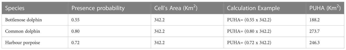
Table 1 Example of PUHA calculation over a single cell unit: the target species presence probability is multiplied by the cell area to obtain PUHA.
2.3.5 Noise impact comparison between the South-western and South-eastern portions of the Black Sea
The Black Sea South-western and South-Eastern regions are very different in terms of traffic and noise: the South-western region has higher ship traffic and higher noise levels, while the South-eastern region has a lower ship traffic, and is therefore much quieter in terms of noise. Since common dolphin regularly occurs in both regions and is the most frequent species, we compared common dolphin relative distribution in equivalent suitable habitat areas in the two regions, which were different only in terms of noise levels.
The hypothesis we wanted to test was that higher noise levels may make the habitat less suitable and therefore affect the species relative abundance. As an index of relative abundance the encounter rate was used, defined in each grid cell as the number of cell sightings divided by the cell effort in kilometres.
For this purpose, an area of 456 cells (108099 km2 or the 23.3% of the Black Sea total area) in the South-western region, and an area of 401 cells in the South-eastern portion (95051 km2 or the 20.5% of the Black Sea total area) were previously identified, and cells with habitat suitability (i.e. species presence probability) greater than 0.6 were selected. Moreover, in order to better compare the suitable habitat, the primary productivity was also considered in terms of remote-sensed concentration of chlorophyll-a (mg m-3, spatial resolution 4 km) available for the year 2019 from the https://giovanni.gsfc.nasa.gov/giovanni/portal. The gridded chlorophyll-a values, in every cell unit, were used as an offset variable and subdivided into two main chlorophyll classes based on the basin median value (i.e. <= 0.593 and > 0.593 mg m-3).
The difference of the species relative abundance in the two regions was assessed by means of a Mann-Whitney independent samples U test (P< 0.05).
3 Results
3.1 Habitat models
The stepwise Binary logistic regression analysis was applied to the three species presence and absence data using depth and seabed slope statistics per cell as possible covariates. Generic Delphinidae sightings were not considered for habitat model development.
3.1.1 Black Sea bottlenose dolphin
Despite the fact that bottlenose dolphin sightings were lower than those of the other two species and more concentrated in the western part of the Black Sea, the species habitat model is decently accurate. The cell effort and mean depth were selected as best predictors for the species presence probability (see Table 2), being respectively a direct and an inverse predictor. Presence probability was in fact inversely proportional to the mean depth and directly proportional to the cell effort (i.e. sum of transect km). The model accuracy (e.g. percent of correct presence and absence classifications) was 89.3% when predicting presence cells and 90.7% when predicting absence cells (see Table 3).
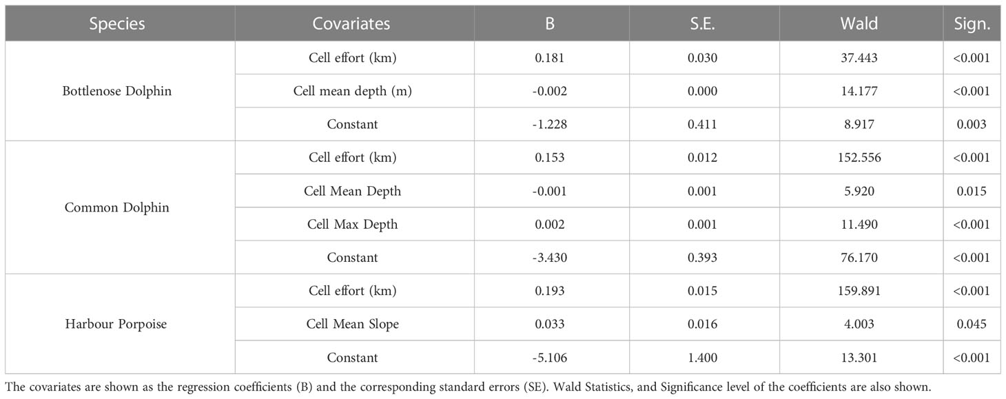
Table 2 Results of the binary logistic regression analysis modelling the presence/absence of Black Sea species.
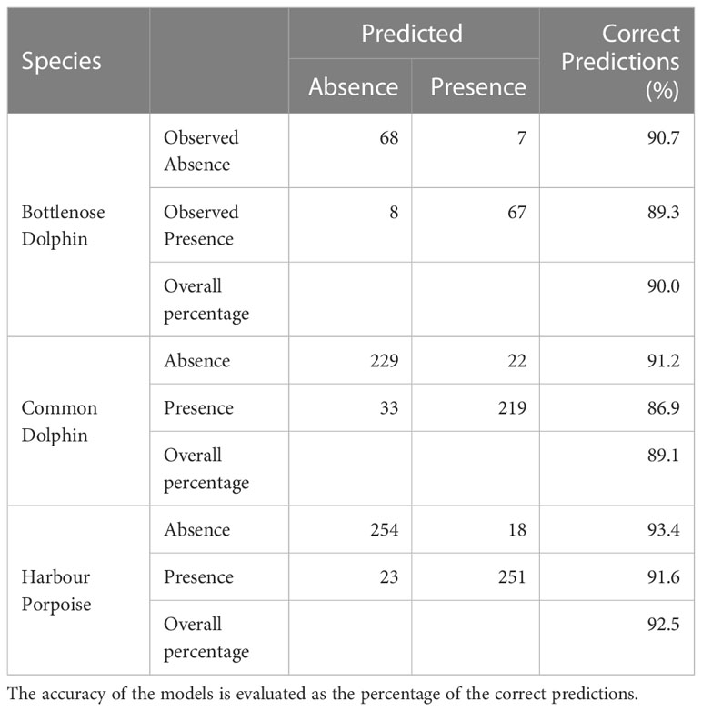
Table 3 Confusion matrix showing the classification performances of the habitat models for predicting presence and absence cell for the three considered species.
Bottlenose dolphin habitat was mainly predicted along the coast, ranging from a bathymetry of 25 and 500 m, with a higher probability in the north-western sector of the Black Sea. In the Azov Sea, where the maximum depth is of the order of 14 m, the habitat is optimal, with high presence probability for the species. In the areas where the continental slope begins and in the central part of the basin, where the depth is greater, the probability of occurrence is instead very low. The total PUHA (sum of each cell PUHA) over the entire Black Sea for this species is 190316 km2 (Figure 3).
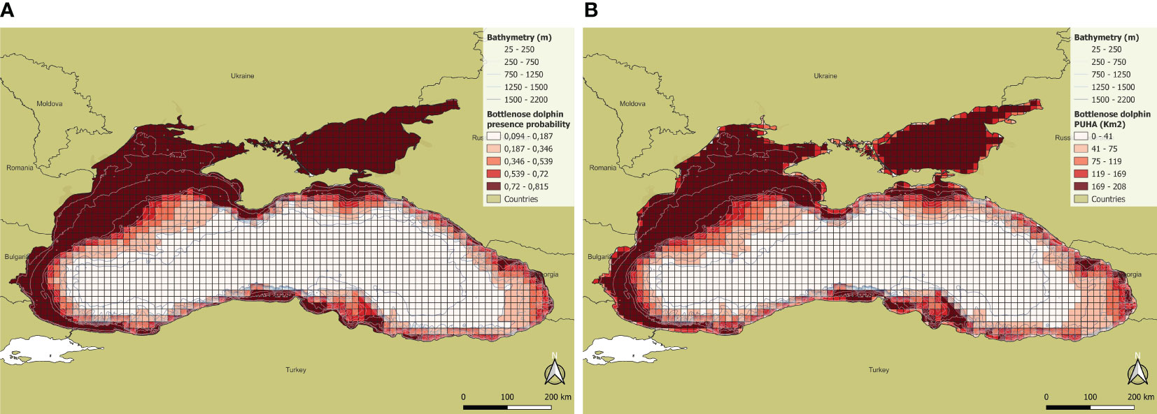
Figure 3 (A) Presence probability and (B) PUHA of Bottlenose dolphin.
3.1.2 Black Sea common dolphin
Sightings of common dolphins were well distributed throughout the study area, providing more data for habitat modelling. The selected predictors for the common dolphin are the cell effort, the cell mean and maximum depth (Table 2). The model exhibited an accuracy of 86.9% when predicting presence cells and 91.2% when predicting absence cells (Table 3). Common dolphin presence was found directly proportional to the effort and to the cell maximum depth, but inversely proportional to the cell mean depth that is the weakest predictor. The results show that the common dolphins are associated with depths between 50 and 2200 m. Along coastal areas, but especially in the north-western zone, between 25 and 100 m, the species probability of occurrence is very low. Likewise, the occurrence probability is low in the Azov Sea, while it is higher in the central and southern portions of the Black Sea basin. The areas with the maximum presence probability (i.e. values between 0.71 and 0.92) are mainly concentrated in Turkish waters, along the continental slope, at depths between 150 and 1750 m. The total PUHA (sum of each cell PUHA) of the species over the entire Black Sea is 231156 km2 (Figure 4).
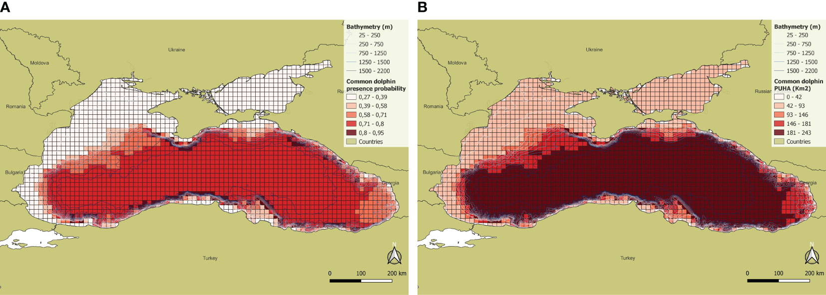
Figure 4 (A) Presence probability and (B) PUHA of Common dolphin.
3.1.3 Black Sea harbour porpoise
Harbour porpoise sightings are well distributed throughout the study area, although more concentrated in the western portion of the Black Sea basin. The selected predictors for the harbour porpoise habitat model are the cell effort and the cell mean sea bed slope (Table 2). The model exhibits an accuracy of 91.6% when predicting presence cells, and of 93.4% when predicting absence cells (Table 3). Harbour porpoises’ presence probability is directly proportional to both the cell effort and the mean sea bed slope. Habitat suitability is higher along the coasts of Bulgaria, Turkey, Georgia and Russia, and in the central portion of the basin. On the other hand, in the north-western area, along the coasts of Ukraine, the presence probability is low, reaching its minimum in the Azov Sea, where the probabilities are close to 0. Harbour porpoises are therefore associated with both shallow and deep waters, between 25 and 2200 m, more precisely from the beginning of the continental slope towards the interior of the basin. The results also show that there is a central-eastern zone where the probability of occurrence decreases since depth increases but the slope decreases. For the harbour porpoise, the calculated PUHA (sum of each cell PUHA) is 274220 km2 (Figure 5).
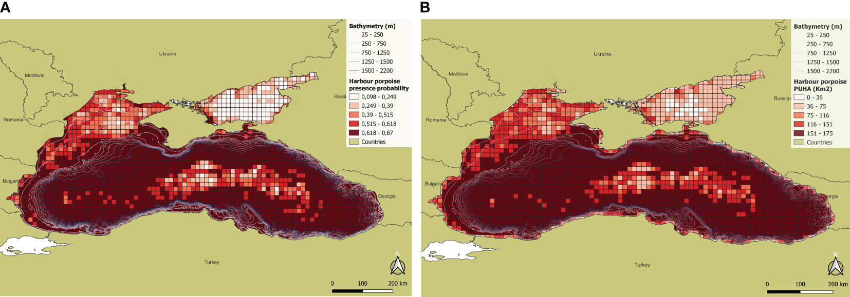
Figure 5 (A) Presence probability and (B) PUHA of Harbour porpoise.
3.2 Noise comparison between the South-western and South-eastern portions of the Black Sea and LOBE validation
In order to test the potential impact of noise on the species’ relative abundance the species encounter rate was tested between the two regions, having equivalent habitat suitability but different noise levels.
Therefore, 364 cells of most suitable habitat (presence probability higher than 0.6) were selected in the South-western area, with 218 sightings, and 295 cells in the South-eastern area, with 240 sightings (Figure 6). As explained in the methods, these cells were also divided per chlorophyll-a classes, resulting respectively for the South-western and the South-eastern regions in 193 cells and 269 cells having chlorophyll-a values lower than the Black Sea July median, and 171 and 26 cells having chlorophyll-a higher than the Black Sea July median.
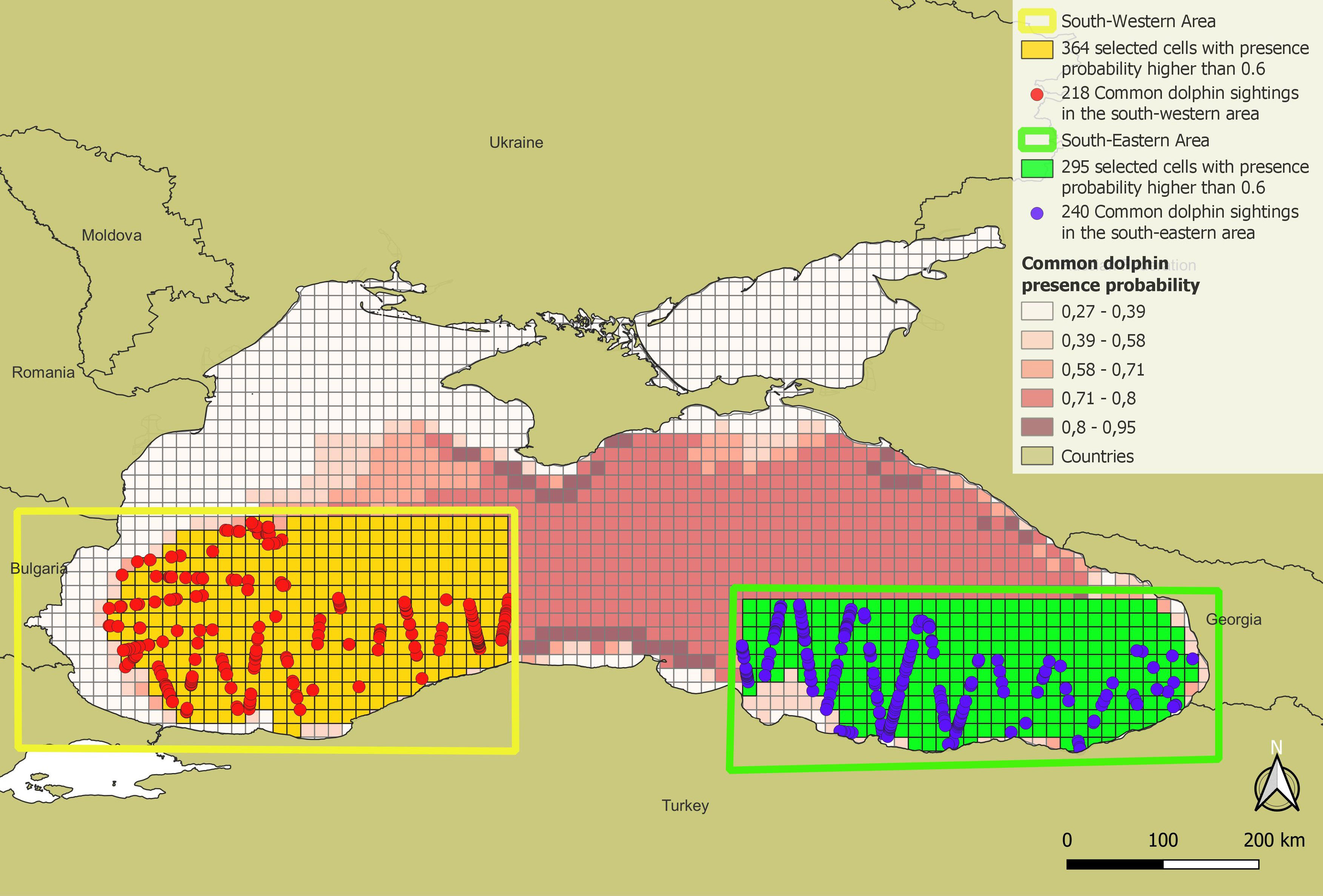
Figure 6 Map of the common dolphin sightings in the cells with optimal habitat suitability (species presence probability higher than 0.6) in the South-western (yellow-enclosed) and South-eastern (green-enclosed) subareas in the Black Sea.
Mann Whitney test showed a significant difference of the encounter rates between the two regions for the lower chlorophyll-a class (Chl-a <= 0.593; U: 807, N: 100; P-value < 0.05) (Figure 7A) while no significant difference was found for the higher chlorophyll-a class (Chl-a > 0.593; U: 49, N: 32; P-value: 0.670) (Figure 7B).
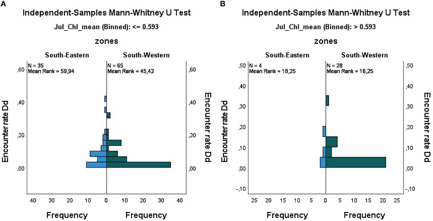
Figure 7 Results of the Mann Whitney Wilcoxon test for common dolphin encounter rate (EncR_Dd) in the South-western and South-eastern regions of the Black Sea. It can be observed that encounter rates are respectively higher in the South-Eastern region in (A) low chlorophyll-a conditions, while they are lower than the South-western encounter rates in (B) high chlorophyll-a conditions.
Particularly, the encounter rate was significantly higher in the South-eastern region when comparing the lower chlorophyll-a conditions (see Table 4).
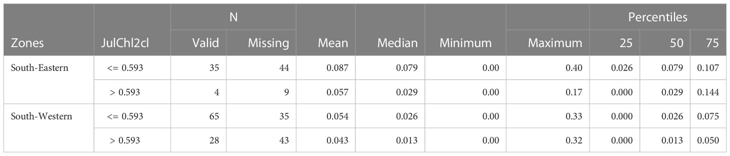
Table 4 Common dolphin encounter rate (EncR_Dd) statistics in the South-western and South-eastern region in lower and higher chlorophyll-a conditions.
Figure 8 shows the comparison of the South-Western and South-Eastern regions in terms of monthly chlorophyll-a average levels. With the exception of a few months (e.g. in Spring and in Autumn) the western primary productivity is higher than in the eastern portion.
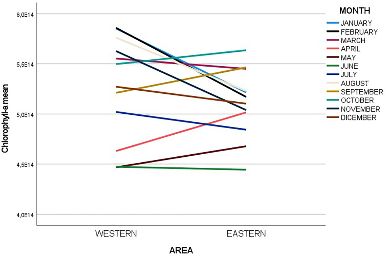
Figure 8 Line graph showing how mean chlorophyll-a concentrations vary over the months of the year 2019 in the selected western and eastern Black Sea regions.
Table 5 shows the average noise levels of the two subregions subdivided by chlorophyll-a class. It can be observed that there is a difference of about 15-17 dB between the South-Western and the South Eastern regions. It is also worthwhile to observe that the higher encounter rates occur in areas where noise levels do not exceed 110 dB. Therefore, grounding on these results, we could assume as LOBE, Level of Onset of the species Biological adverse Effect (i.e. the encounter rate decrease), an SPL ranging between 110 dB (50th grid cell percentile of the median SPLs) and 120 dB (75th grid cell percentile of the 95th SPLs).
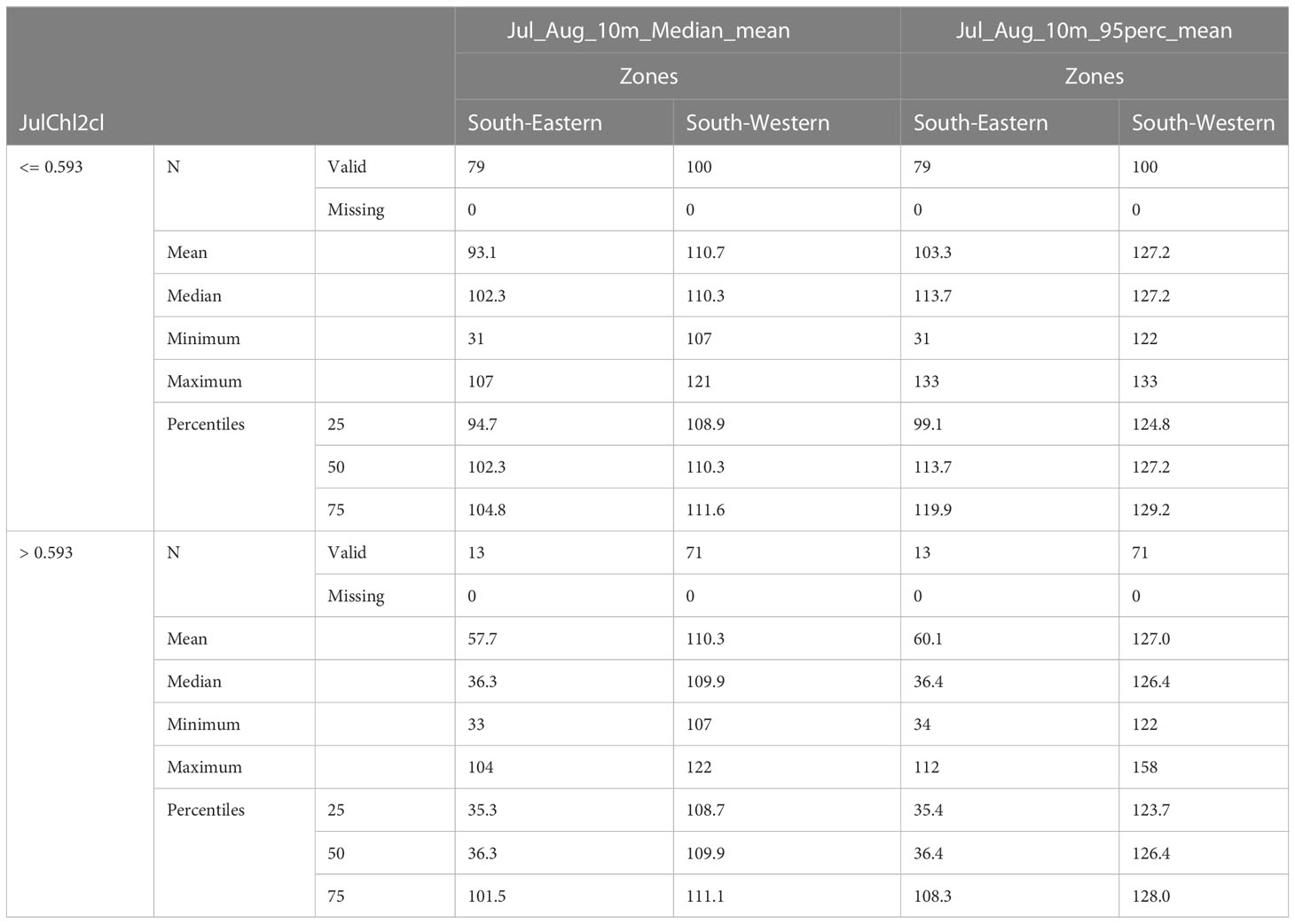
Table 5 Noise level (SPL re 1 μPa) statistics are shown for the common dolphin suitable habitat in the South-Western and in the South-Eastern regions at the different primary production conditions (i.e. Chl-a).
3.3 Noise impact assessment
The amount of habitat negatively impacted by underwater noise for each of the three target species was assessed as described in the Methods, combining the relevant noise maps with the habitat models and the derived PUHA. The simulated noise map shows where the presence of harbours causes higher noise (Figure 9A). The obtained noise maps are coherent with the ship traffic density maps available from the Emodnet portal for the year 2019 (Source: https://www.emodnet-humanactivities.eu/), Figure 9B.
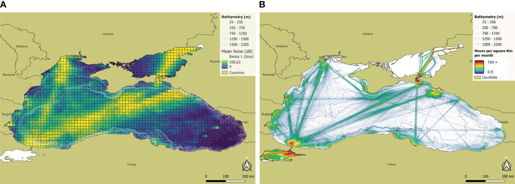
Figure 9 (A) Noise map showing mean SPL values (dB re 1μPa) per cell using the grid of 10 x 10 nm; (B) Mean vessel density for 2019 (hours per square Km per month, Source: https://www.emodnet-humanactivities.eu).
As already explained, the areas with the highest noise levels are mainly located in the South-western portion of the basin, while in the South-eastern portion noise is lower. The grid cells (501 cells) having a noise level higher than LOBE (i.e. SPL above 110 dB re 1 μPA), in the Black Sea occupy 25.16% of the basin area (2069 cells). Most of the “impacted” cells are located along the main traffic routes in the basin, especially in the South-western portion, while no “impacted” cells are present in the South-eastern portion of the basin. Finally, risk maps were created from which the percentages of Potentially Usable Habitat Area (PUHA) exposed to noise levels above LOBE were quantified for the target species (Figure 10).
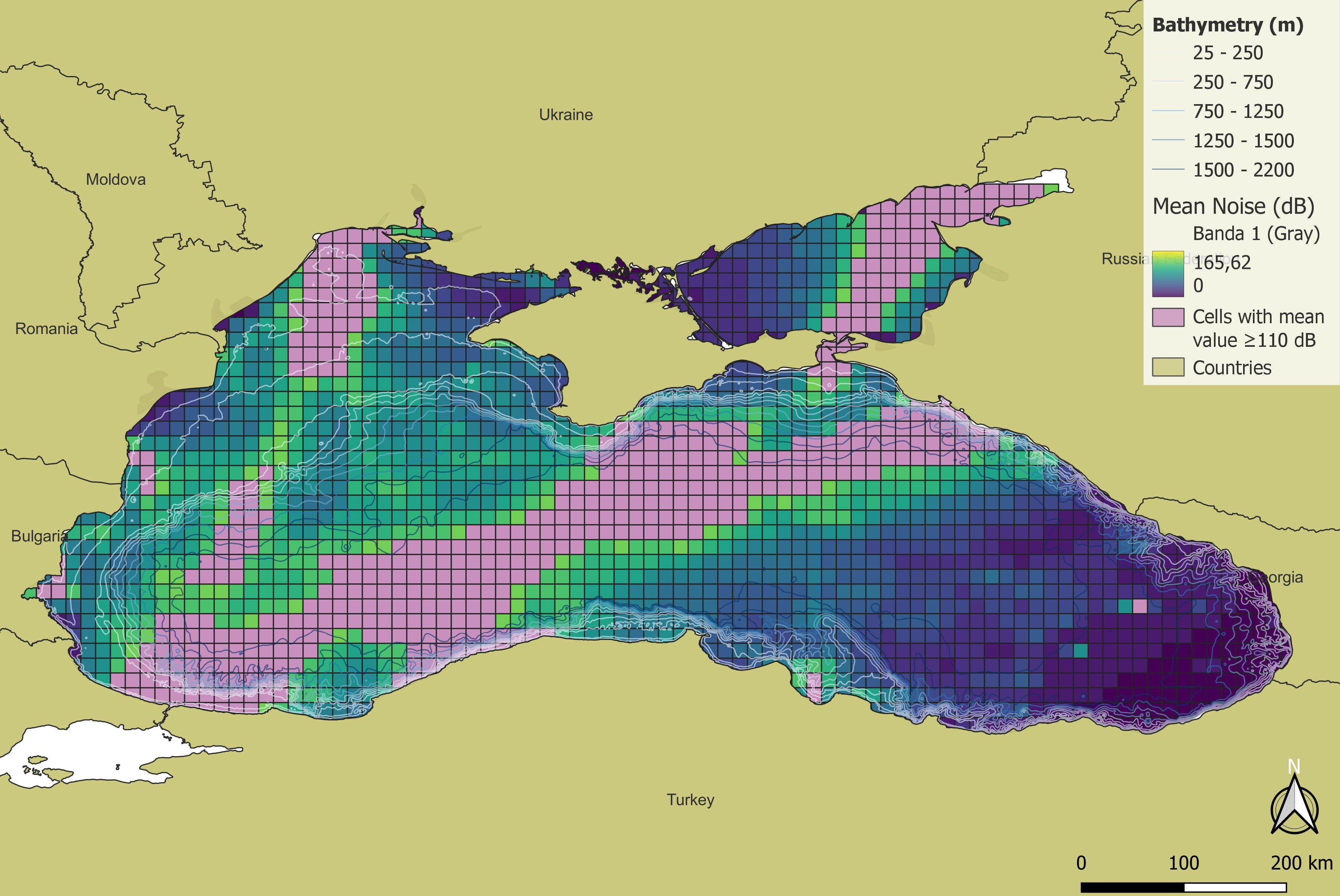
Figure 10 Noise Risk maps showing the pink the grid cells where noise levels are higher than LOBE equal to 110 dB re 1 μPa (501 cells, corresponding to 25.16% of Black Sea total area).
The results also show that the percentages of impacted PUHA are very similar for the three species considered. As far as the bottlenose dolphin is concerned, the percentage of impacted PUHA was 21.4%, which is not unexpected for a species regularly occurring in the coastal areas, where ship traffic and related noise are generally higher. The pelagic areas in the Black Sea having noise levels greater than LOBE do not impact too much on the species PUHA since the species presence probability in the pelagic area is very low (Figure 11A). The percentage of impacted PUHA is higher for harbour porpoise (24.46%), since the species’ suitable habitat is concentrated along the southern coasts and in the central areas of the basin where the noise levels more frequently exceed LOBE (Figure 11C). But the highest percentage of impacted PUHA was found for common dolphin (26.47%), being the species habitat suitability higher in the central portion of the basin, corresponding to the area of the main shipping lanes (Figure 11B).
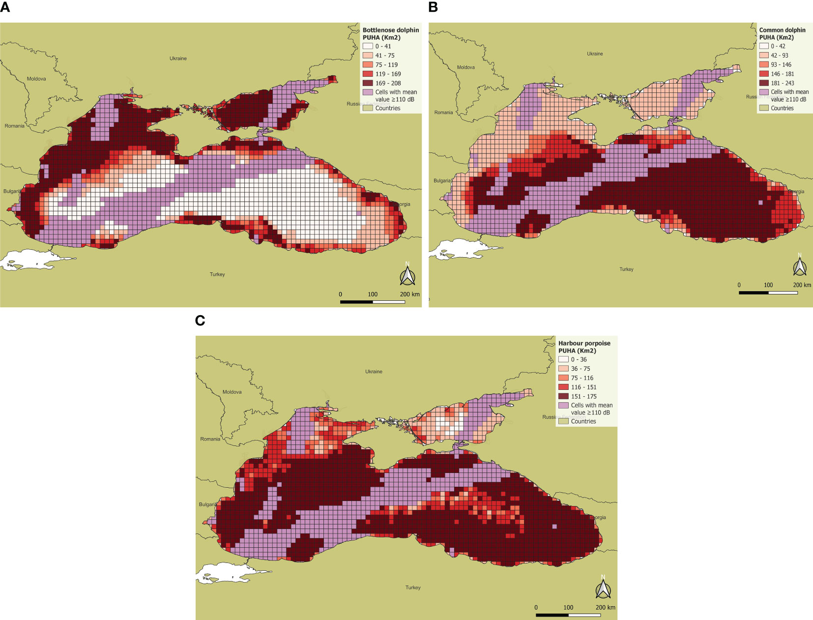
Figure 11 PUHA of the three Black Sea cetacean species where pink cells indicate mean noise values equal to or greater than 110 dB: (A) Bottlenose dolphin; (B) Common dolphin; (C) Harbour porpoise.
4 Discussion
This study presents a modelling approach for estimating the Potentially Usable Habitat Area (PUHA) of the three cetacean species regularly occurring in the Black Sea. The models were developed on the basis of the large scale data collection acquired through the EU-funded CeNoBS project, in collaboration with and co-funded by ACCOBAMS under the ACCOBAMS Survey Initiative (ACCOBAMS, 2021a; Paiu et al., 2021). The study shows how physiographic predictors may play an important role in predicting the potential distribution and habitat preferences of cetaceans.
The developed habitat suitability models exhibited high accuracies (between 89% and 92%) in predicting the presence/absence of the considered species in the Black Sea, demonstrating that these species have very specific habitat preferences.
The bottlenose dolphin is among the best known, most widespread and studied cetacean species in all seas, with habitat preferences in Mediterranean Sea being mostly reported in coastal and shallow waters (e.g. Gnone et al., 2011; Azzellino et al., 2012). Black Sea bottlenose dolphins show habitat preferences in line with this common pattern, the optimal depths ranging between 25 and 500 m depth. The model shows that bottlenose dolphins are more likely to be found in coastal areas, especially in the north-western part, while in the central zone of the basin, at greater depths (over 750 m), and in areas where the continental slope begins, the probability of their presence is much lower. These results are in agreement with those obtained by Sánchez-Cabanes et al. (2017) in the same area, which showed a preference for habitats along the coast but at slightly shallower water depths, between 50 and 250 m. Paiu et al. (2021) also showed a higher abundance in coastal areas, and in the western part of the Black Sea. Numerous other studies (e.g. Cañadas et al., 2002; Gnone et al., 2011; Azzellino et al., 2012; Marini et al., 2015; Carlucci et al., 2016; Giannoulaki et al., 2017; Affinito et al, 2019; Muckenhirn et al., 2021) show that the areas of greatest bottlenose dolphin presence are associated with coastal areas at depths up to 40-600 m. In the Black Sea, however, the species’ higher preference for shallow-water habitats may also be the consequence of the deep anoxic waters and the consequent lack of prey. In deep water, no sightings of bottlenose dolphins have been detected and the predicted presence probability is close to zero, in agreement with the study of Sánchez-Cabanes et al. (2017) which has approximately the same spatial coverage but is based on data deriving from opportunist surveys. The same authors refer that the species distribution changed in time since it was known that in the 1960s and 1970s, bottlenose dolphins were also reported in the deep central part of the basin. Sánchez-Cabanes and colleagues speculated that the current distribution shift could be the effect of the ecosystem changes occurred in the last decades which may have prompted the species to change its diet and consequently distribution. Another possible explanation might be related to fisheries which, before being regulated, led to a decline in pelagic fish, thus impacting both prey availability and feeding behaviour of bottlenose dolphins. It is known, in fact, that bottlenose dolphins may change their habitat preferences depending on the presence of prey (Hastie et al., 2004).
The common dolphin is another widespread dolphin species with a variety of habitats, showing greater preferences for deep sea areas and continental shelves (Cañadas and Hammond, 2008). Present study shows greater species presence in deeper waters, with high presence probability associated to areas between 150 and 1750 m, relative to the continental slope. In the north-western region and in the Azov Sea, where there are medium- and -shallow-water depths but minimal slope values, the species probability of occurrence reports very low values (between 0.24 and 0.34). These results also agree with those obtained by Sánchez-Cabanes et al. (2017), whose models showed greater presence for the central part of the basin between the bathymetries of 50 and 2250 m and in waters between 5-18°C, which corresponds to the waters of the southern zone towards the central zone of the basin, away from the north-western continental shelves, where the probability is indeed lower (Shapiro et al., 2010). The results also agree with the abundance studies of the CeNoBS project, which predict a higher abundance towards the central zone and along the continental shelf (Paiu et al., 2021). In addition, other former studies reported a prevalence of the common dolphin mainly in the central part of the Black Sea (Raykov and Panayotova, 2012; Radu et al., 2013; Birkun et al., 2014), suggesting that the species habitat preferences at least in the last two decades have not changed over time. Also in other areas, such as the Northeast Atlantic and the Mediterranean Alboran Sea, this species shows a preference for deep waters, between 400 and 2000 m (Cañadas et al., 2002; Cañadas et al., 2009). As with bottlenose dolphins, common dolphins are also closely linked to the presence of prey. In fact, they prefer pelagic fish in particular Clupeidae and Engraulidae, which are mainly found in the continental shelf areas (Cañadas et al., 2002). Furthermore, the movement and aggregation of fish due to currents and tides attract the common dolphin (Paradell et al., 2019) linking their distribution to prey migrations (Dede and Tonay, 2010; Radu et al., 2013).
The harbour porpoise is a widespread species in the colder, coastal waters of the North Pacific, North Atlantic, and Black Sea (Bjorge et al., 2018). It has also been observed in the western Mediterranean (Cañadas et al., 2005) and northern Aegean Sea (Cucknell et al., 2016). Patterns show a preference for meridional coastal waters, as well as southwestern and southeastern ones, while occurrence values decrease in the northern part of the basin. The slope is an excellent predictor, as the preferences just described refer to the areas where the continental shelf begins and where the mean slope values per cell are highest. For example, within the central eastern part of the basin and in the Sea of Azov, the presence values are lower as the slope tends to decrease. The harbour porpoise is therefore present in both shallower and pelagic waters, with a depth range between 25 and 2200 m. As far as Black Sea Harbour porpoise is concerned this study habitat models only partially agree with the ones presented by Sánchez-Cabanes et al. (2017), which predict a greater presence in shallow waters below 200 m with preferences for shelf waters between 50 and 150 m, and a predicted habitat similar to that of bottlenose dolphins. However this discrepancy could be the effect of the effort bias deriving from the opportunistic surveys which are the source of their dataset. Birkun et al. (2014) also predicted a secondary habitat in the open sea (deeper than 200 m) in agreement with the results obtained here. In the Azov Sea Birkun et al.’s models also predicted a good probability, agreeing with previously described seasonal migrations in which harbour porpoises occupy the Azov Sea during the warmer months (Kleinenberg, 1956), and abandoning it during the winter (Tzalkin, 1938). Studies in the Atlantic and Pacific Ocean show the presence of harbour porpoise in shallow waters between 20 and 50 m up to a maximum of 150-200 m, bathymetrics corresponding to continental slopes (Read and Westgate, 1997; Raum-Suryae and Harvey, 1998; Marubini et al., 2009; Isojunno et al., 2012). Minor preferences within this range are in waters deeper than 100 m (Carretta et al., 2001; Embling et al., 2010; Isojunno et al., 2012). In Greenland, however, harbour porpoises have been found moving to deeper habitats during winter periods by diving in waters above 400 m (Stalder et al., 2020). In the Black Sea the interspecific competition may have led to a change in harbour porpoise feeding habits favouring more pelagic prey. Harbour porpoises in fact usually feed on both benthic fish found in shallow waters and pelagic fish (Krivokhizhin and Birkun, 2006; Tonay et al., 2007). Moreover, in addition to the relevance of the habitat models for the better understanding of the species ecology, the possibility to predict the species’ potentially usable habitat (PUHA) offers also a great opportunity for assessing the extent of the species habitat which is affected by potentially harmful noise levels, and it may also support the identification of the Level of Onset of Biological adverse Effects, LOBE. By predicting the areas with the highest likelihood of the species presence, habitat models may in fact support their risk exposure assessment to different anthropogenic pressures such as military sonars, shipyard work, vessel traffic, etc. (Azzellino et al., 2012).
In this study, it has been shown how habitat models predictions, combined with noise maps produced through specific shipping noise models, allow to estimate the potential impact of continuous anthropogenic noise on the species potential habitat availability (e.g. PUHA). Vessel traffic is considerably high in the Black Sea, especially in the vicinity of the main ports, along the Western coast and across the basin, as reflected by the corresponding noise maps. Considering as LOBE an SPL of 110 dB re 1 μPa for the 63 Hz one-third octave band these noise levels are more concentrated along the routes crossing the basin, connecting the ports of Istanbul, Odessa, Zonguldak, Mariupol and Rostov. It is therefore explainable that the species having the largest portion of impacted habitats are the common dolphin (26.5%) and the harbour porpoise (24.5%), both of which are present in the central part of the basin and in relatively deep waters. The bottlenose dolphin, being more coastal and concentrated in the Western basin shows a slightly lower portion of impacted habitat area, since the species habitat is only limitedly impacted by the shipping routes present in the central part. However, the percentages of impacted habitat area for the three species are overall relatively high, affecting important areas where cetaceans carry out their main survival activities, such as foraging, reproduction and socialisation. Analyses carried out for the western and eastern areas, where traffic and noise data have different values, show that, in any case, common dolphin and harbour porpoise are more present in the western part where noise is higher. This could mean that, although the noise is high, these cetacean species can still manage to use the area. Chlorophyll concentration data clearly show that the Western basin is significantly more productive than the Eastern basin, especially in the summer months (i.e. June and July). The common dolphin has been reported to prefer highly productive areas (Fiedler and Reilly, 1994) and to have larger groups in areas with higher chlorophyll concentrations (Cañadas and Hammond, 2008). As far as harbour porpoises are concerned, several studies have also found a greater species presence in areas with higher chlorophyll and nutrient gradients (Wingfield et al., 2017). In the study by Stalder et al. (2020), anomalies regarding high chlorophyll concentrations in certain areas seem to explain the movements and aggregations of harbour porpoises, as these areas possess oceanographic features that can accumulate primary consumers, making them important foraging areas. In some habitat models built for harbour porpoises in which dynamic predictors, such as sea state temperature (SST) and chlorophyll concentration, were considered in addition to static predictors (depth and slope), chlorophyll turns out to be a very good predictor of harbour porpoise presence (Gilles et al., 2011). This would seem coherent with our results showing that although noise and traffic levels are high in the Western basin, the target species still use these areas because there is a high primary productivity and they have adapted to tolerate the noise levels present. Several studies have documented cetacean adaptation capabilities to noise, especially with regard to vocalisations and their masking. In fact, many cetacean species appear to have increased frequencies in the emission of vocalisations to continue communicating with conspecifics even in places where noise has become increasingly loud (Lesage et al., 1999; May-Collado and Wartzok, 2008; Parks, 2012). Noise ‘tolerance’ could be the result of various contexts such as the absence of habitat, excessive costs related to avoidance or, as hypothesised here, the need for individuals and populations to remain in the area (Wright et al., 2007). Such adaptation to loud noise levels is in fact an additional challenge to assess noise effect. The habitat models developed in this study enabled also to design a methodological approach to assess noise impact: equivalent suitable and productive habitats with different noise levels have been in fact compared between the South-Western and the South-Eastern portions of the Black Sea, showing that the noisier habitats have a significantly lower common dolphin encounter rate. It is noteworthy to underline that the statistical difference could be assessed only for suitable habitats having a primary productivity lower than the Black sea median (chl-a <= 0.539) while there was no statistical difference between high productivity (chl-a > 0.539) suitable habitats.
This result suggests that species have a tendency to avoid environments with high levels of noise when it is not crucial for their foraging activities. However, they demonstrate adaptability when high noise levels coincide with critical foraging habitats. It’s important to note that the sample size for the high productivity habitats was significantly limited, particularly in the South-Western basin where cells with such high primary productivity are rare.
It is important to note that noise pollution is not the sole stressor arising from shipping activities. While there is limited documentation on collision risks for dolphins (Schoeman et al., 2020), the avoidance of collisions could be an additional factor that is challenging to separate from noise pollution. Dolphins may tend to avoid areas with high ship traffic to minimize the risk of collisions rather than solely avoiding noise pollution, making it difficult to disentangle the effects of these two factors.
Nevertheless, it is crucial to emphasize that when comparing the noise levels of low productivity cells with the same habitat suitability between the South-Western and the South-Eastern regions (as shown in Table 5), the sound pressure level (SPL) at which the biological response of the species, indicated by a decrease in encounter rate, was presumed to occur ranged from a median noise level of 110 dB to a 95th percentile noise level of 120 dB. This evidence strongly suggests that this noise range can be considered a reasonable Level of Onset of Biological adverse Effects (LOBE).
5 Conclusion
Large-scale synoptic surveys have proven to be valuable and functional for modeling the presence/absence of cetaceans and generating habitat suitability models. Aerial surveys of this nature can effectively bridge data gaps, particularly in areas where even long-term surveys exhibit limitations, thereby providing additional information on Black Sea populations. This study demonstrates the effectiveness of physical predictors, such as depth and seabed slope, in predicting the potential distribution and habitat preferences of cetaceans.
These habitat models are highly valuable for assessing the impact of anthropogenic pressures, such as shipping noise, on specific areas. They can support management efforts by identifying critical habitats that require special protection, thus enhancing local and regional management strategies. Additionally, the application of habitat models facilitates the assessment of species’ exposure and risk to noise. It enables the implementation of methodologies, such as the proposed assessment of MSFD D11, and evaluation of the need for mitigation measures such as ship traffic reduction or vessel speed limits in critical areas. These models can also help establish noise levels that should not be exceeded to avoid adverse effects on the populations of the target species (e.g., LOBE).
This study specifically suggests that a sound pressure level (SPL) at a frequency of 63Hz ranging from a median noise level of 110 dB to a 95th percentile noise level of 120 dB can be considered as the threshold for the biological response of the target species (common dolphin), resulting in a decrease in encounter rate. Further investigations and studies are necessary to provide additional evidence supporting this LOBE value and to extend the study to other target species. Nonetheless, the methodology demonstrated in this study, which utilizes habitat models to select equivalently suitable habitats that differ only in noise levels, will be valuable for controlling potential confounding factors when assessing the effects of noise.
Data availability statement
The original contributions presented in the study are included in the article/supplementary material. Further inquiries can be directed to the corresponding author.
Author contributions
Writing—original draft preparation: VF. Writing—review and editing: AM, AP, AA. Designing the case study: AA and VF. Provided conceptual details on the realisation of the habitat models: AA. Involved in the realisation of noise maps for the case study: AM. Involved in the organisation and data collection of the CeNoBS project: R-MP. Provided conceptual details on the creation of noise maps and risk assessment: AA, AP, AM and NO. All authors provided comments to improve the manuscript. All authors contributed to the article and approved the submitted version.
Funding
The presented study was financed by Directorate-General for Environment, European Commission (DG Environment) through the QUIETSEAS project (agreement 110661/2020/839603/SUB/ENV.C.2. https://quietseas.eu/, access on 16 November 2022) within the call “DG ENV/MSFD 2020”.
Acknowledgments
The authors wish to thank the partners who provided their comments to the QUIETSEAS deliverables which are at the basis of the presented methodology: CTN, ACCOBAMS, HCMR, IzVRS, SPA/RAC, MHD, DFMR and SHOM. Many thanks also to the reviewers who contributed to significantly improve the paper.
Conflict of interest
The authors declare that the research was conducted in the absence of any commercial or financial relationships that could be construed as a potential conflict of interest.
Publisher’s note
All claims expressed in this article are solely those of the authors and do not necessarily represent those of their affiliated organizations, or those of the publisher, the editors and the reviewers. Any product that may be evaluated in this article, or claim that may be made by its manufacturer, is not guaranteed or endorsed by the publisher.
Footnotes
- ^ ACCOBAMS: The Agreement on the Conservation of Cetaceans of the Black Sea, Mediterranean Sea and contiguous Atlantic area.
- ^ CeNoBS: Support MSFD implementation in the Black Sea through establishing a regional monitoring system of cetaceans (D1) and noise monitoring (D11) for achieving Good Environmental Status.
References
Abel O. (1905). Eine stammtype der delphiniden aus dem miocän der halbinsel taman. jahrbuch der kaiserlich-königlichen geologischen reichsanstalt. Jahrb. der Kais. Geol. Reichsanstalt. 55, 375–392.
ACCOBAMS (2021a). Estimates of abundance and distribution of cetaceans in the Black Sea from 2019 surveys. Eds. Paiu R. M., Panigada S., Cañadas A., Gol’din P., Popov D., David L., Amaha Ozturk A., Glazov D. (Monaco: ACCOBAMS - ACCOBAMS Survey Initiative/CeNoBS Projects). 54 pages.
ACCOBAMS (2021b). Conserving Whales, Dolphins and Porpoises in the Mediterranean Sea, Black Sea and adjacent areas: an ACCOBAMS status report, (2021). Eds. Notarbartolo di Sciara G., Tonay A. M. (Monaco: ACCOBAMS). 160 p.
ACCOBAMS (2023). Progress in the assessment/re-assessment of the iucn status of cetacean species in the accobams area (Tunisia: Fifteenth meeting of the scientific committee 10 and 11 May 2023 - Tunis).
Affinito F., Olaya M. C., Akkaya B. A., Brill D., Whittaker G., Capel L. (2019). On the behaviour of an under-studied population of bottlenose dolphins in the Southern Adriatic Sea. J. Mar. Biol. Assoc. United Kingdom 99 (4), 1017–1023. doi: 10.1017/S0025315418000772
Anderwald P., Evans P. G. H., Gygax L., Hoelzel A. R. (2011). Role of feeding strategies in sea bird minke whale associations. Mar. Ecol. Prog. Ser. 424, 219–227. doi: 10.3354/meps08947
Azzellino A., Frassà V., Prospathopoulos A., Lajaunie M., Ollivier O., Lueber S., et al. (2023). “Deliverable 5.2 - proposal of a methodology to establish thresholds values for D11C2 in the mediterranean and black sea regions,” in QUIETSEAS project, 36. Available at: https://quietseas.eu/project-work-plan/#outputs.
Azzellino A., Airoldi S., Gaspari S., Nani B. (2008). Habitat use of cetaceans along the continental slope and adjacent waters in the western Ligurian Sea. Deep Sea Res. Part I 55, 296–323. doi: 10.1016/j.dsr.2007.11.006
Azzellino A., De Santis V., Lanfredi C., Prospathopoulos A., Kassis D., Felis I., et al. (2021) D 6.2 “Joint proposal of a methodology to establish thresholds values for impulsive noise in the Mediterranean Sea Region” QuietMED2 deliverable. Available at: https://quietmed2.eu/outputs/ (Accessed 28.03.2023).
Azzellino A., Lanfredi C., D’Amico A., Pavan G., Podestà M., Haun J. (2011). Risk mapping for sensitive species to underwater anthropogenic sound emissions: model development and validation in two Mediterranean areas. Mar. pollut. Bull. 63, 56–70. doi: 10.1016/j.marpolbul.2011.01.003
Azzellino A., Panigada S., Lanfredi C., Zanardelli M., Airoldi S., Notobartolo di Sciara G. (2012). Predictive habitat models for managing marine areas: spatial and temporal distribution of marine mammals within the Pelagos Sanctuary (Northwestern Mediterranean Sea). OceanCoast. Manag 67, 63–74. doi: 10.1016/j.ocecoaman.2012.05.024
Balkas T., Decev G., Mihnea R. (1990). “State of the Marine Environment in the Black Sea Region,” in Regional Seas Reports and Studies, No: 124, vol. 40. (Nairobi: UNEP).
Barabash I. I. (1935). Delphinus delphis ponticus subsp. Bull. Mosk Obs Ispyt Prir (Bulletin Moscow Soc. Nat. New Ser. 44, 246–249. (In Russian with English summary).
Barabash-Nikiforov I. I. (1940). Cetacean fauna of the black sea. its composition and origin (Voronezh: Voronezh University Publ.), 86. (in Russian).
Baş A. A., Öztürk B., Öztürk A. A. (2019). Encounter rate, residency pattern and site fidelity of bottlenose dolphins (Tursiops truncatus) within the Istanbul Strait, Turkey. Journal of the Marine Biological Association of the United Kingdom, 99 (4),1009–1016.doi: 10.1017/S0025315418000577
Baumgartner M. F. (1997). The distribution of Risso's dolphin (Grampus griseus) with respect to the physiography of the northern Gulf of Mexico. Mar. Mammal Sci. 13, 614–638. doi: 10.1111/j.1748-7692.1997.tb00087.x
Birkun A. J. (2002). “Cetacean direct killing and live capture in the Black Sea,” in Cetaceans of the Mediterranean and Black Seas: state of knowledge and conservation strategies, vol. 6 . Ed. Notarbartolo di Sciara G. (Monaco: A report to the ACCOBAMS Secretariat), 10.
Birkun A. J. (2012). “Tursiops truncatus ssp. ponticus,” in IUCN 2013. IUCN Red List of Threatened Species. Version 2013.2. Available at: www.iucnredlist.org.
Birkun A. J., Frantzis A. (2008). “Phocoena phocoena ssp. relicta,” in IUCN 2013. IUCN Red List of Threatened Species. Version 2013.2.
Birkun A. J., Krivokhizhin S. V., Glazov D. M. (2004). “Abundance estimates of cetaceans in coastal waters of the northern Black Sea: results of boat surveys in August-October 2003,” in Marine Mammals of the Holartic, Collection of Scientific Papers. Ed. Belkovich V. M. (Moscow: KMK Scientific Press), 64–71.
Birkun A. J., Northridge S. P., Willsteed E. A., James F. A., Kilgour C., Lander M., et al. (2014). Studies for carrying out the Common Fisheries Policy: adverse fisheries impact on cetacean populations in the Black Sea (Brussels: Final report to the European Commission), 1–347.
Blasi M., Boitani L. (2012). Modelling fine-scale distribution of the bottlenose dolphin Tursiops truncatus using physiographic features on Filicudi (southern Thyrrenian Sea, Italy). Endag. Species Res. 17, 269–288. doi: 10.3354/esr00422
Buckland S. T., Rexstad E. A., Marques T. A., Oedekoven C. S. (2015). “Distance Sampling: sMethods and Applications,” in Series Methods in Statistical Ecology, vol. 2015. (Switzerland: Springer International Publishing). doi: 10.1007/978-3-319-19219-2
Buckland S. T., Smith T. D., Cattanach K. L. (1992). “Status of small cetacean populations in the Black Sea: Review of current information and suggestions for future research,” in Report Of The International Whaling Commission (The International Whaling Commission) 42, 513–516.
Cañadas A. M., Donovan G. P., Desportes G., Borchers D. L. (2009). A short review of the distribution of short-beaked common dolphins (Delphinus delphis) in the central and eastern North Atlantic with an abundance estimate for part of this area Vol. 7 (NAMMCO Scientific Publications). 7, 201–220. Available at: 10.7557/3.2714.
Cañadas A., Hammond P. S. (2008). “Abundance and habitat preferences of the short-beaked common dolphin Delphinus delphis in the southwestern Mediterranean: implications for conservation,” in Endangered Species Research (ESR). 4 (3), 309–331. doi: 10.3354/esr00073
Cañadas A., Sagarminaga R., De Stephanis R. (2005). Habitat selection modelling as a conservation tool: proposals for marine protected areas for cetaceans in southern Spanish waters. Aquat. Conserv. 15, 495–521. doi: 10.1002/aqc.689
Cañadas A., Sagarminaga R., Garcıa T. S. (2002). Cetacean distribution related with depth and slope in the Mediterranean waters off southern Spain. Deep Sea Res. 49, 2053 –2073. doi: 10.1016/S0967-0637(02)00123-1
Carlucci R., Fanizza C., Cipriano G., Paoli C., Russo T., Vassallo P. (2016). Modeling the spatial distribution of the striped dolphin (Stenella coeruleoalba) and common bottlenose dolphin (Tursiops truncatus) in the Gulf of Taranto (Northern Ionian Sea, Central-eastern Mediterranean Sea). Ecol. Indic. 69, 707–721. doi: 10.1016/j.ecolind.2016.05.035
Carretta J. V., Taylor B. L., Chivers S. J. (2001). Abundance and depth distribution of harbour porpoise (Phocoena phocoena) in northern California determined from 1995 ship survey. Fish. Bull. 99, 29–39.
Cribb N., Miller C., Seuront L. (2015). Towardsa standardized approach of Cetacean habitat: past achievements and future directions. Open J. Mar. Sci. 5, 335–357. doi: 10.4236/ojms.2015.53028
Cucknell A. C., Frantzis A., Boisseau O., Romagosa M., Ryan C., Tonay A. M., et al. (2016). Harbour porpoises in the Aegean Sea, Eastern Mediterranean: the species’ presence is confirmed. Mar. Biodiversity Records 9, 72. doi: 10.1186/s41200-016-0050-5
Davis R. W., Ortega-Ortiz J. G., Ribi C. A., Evans W. E., Biggs D. C., Ressler P. H., et al. (2002). Cetacean habitat in the northern oceanic Gulf of Mexico. Deep-Sea Res. 49, 121–142. doi: 10.1016/S0967-0637(01)00035-8
Dede A., Tonay A. M. (2010). Cetacean sightings in the Western Black Sea in autumn 2007. J. Environ. Prot. Ecol. 11, 1491–1494.
Embling C. B., Gillibrand P. A., Gordon J. (2010). Using habitat models to identify suitable sites for marine protected areas for harbour porpoises (Phocoena phocoena). Biol. Conserv. 143, 267–279. doi: 10.1016/j.biocon.2009.09.005
Ferguson M. C., Barlow J. (2001). Spatial distribution and density of cetaceans in the eastern tropical Pacific Ocean based on summer/fall research vessel surveys in 1986 e 96. Southwest fisheries science center. La Jolla, 1–4. (Addendum). Available at: https://repository.library.noaa.gov/view/noaa/3394.
Ferguson M. C., Barlow J., Fiedler P., Reilly S. B., Gerrodette T. (2006a). Spatial models of delphinid (family Delphinidae) encounter rate and group size in the eastern tropical Pacific Ocean. Ecol. Model. 193, 645–662. doi: 10.1016/j.ecolmodel.2005.10.034
Ferguson M. C., Barlow J., Reilly S. B., Gerrodette T. (2006b). Predicting Cuvier’s (Ziphius cavirostris) and Mesopolodon beaked whale population density from habitat characteristics in the eastern tropical Pacific Ocean. J. Cetacean Res. Manage 7 (3), 287–299. doi: 10.47536/jcrm.v7i3.738
Fiedler P. C., Reilly S. B. (1994). Interannual variability of dolphin habitats in the eastern tropical Pacific. II: Effects on abundances estimated from tuna vessel sightings, 1975-1990. Fish. Bull. 92, 434–450.
Forney K. A., Ferguson M. C., Becker E. A., Fiedler P. C., Redfern J. V., Barlow J., et al. (2012). Habitat-based spatial models of cetacean density in the eastern Pacific Ocean. Endanger. Species Res. 16 (2), 113–133. doi: 10.3354/esr00393
Frankel A. S., Clark C. W., Herman L. M., Gabriels C. M. (1995). Spatial distribution, habitat utilization, and social interactions of humpback whales, Megaptera novaeangliae, off Hawaii determined using acoustic and visual means. Can. J. Zool 73, 1134–1146. doi: 10.1139/z95-135
Giannoulaki M., Markoglou E., Valavanis V. D., Alexiadou P., Cucknell A., Frantzis A. (2017). Linking small pelagic fish and cetacean distribution to model suitable habitat for coastal dolphin species, Delphinus delphis and Tursiops truncatus, in the Greek Seas (Eastern Mediterranean). Aquat. Conserv: Mar. Freshw. Ecosyst. 27, 436–451. doi: 10.1002/aqc.2669
Gilles A., Adler S., Kaschner K., Scheidat M., Siebert U. (2011). Modelling harbour porpoise seasonal density as a function of the German Bight environment: implications for management. Endang Species Res. 14, 157–169. doi: 10.3354/esr00344
Gladilina E. V., Gol’din P. E. (2016). Abundance and summer distribution of a local stock of black sea bottlenose dolphins, tursiops truncatus (Cetacea, delphinidae), in coastal waters near sudak. Vestnik zoologii 50, 49–56. doi: 10.1515/vzoo-2016-0006
Gladilina E. V., Vishnyakova K. A., Neprokin O. O., Ivanchikova Y. F., Derkacheva T. A., Kryukova A. A., et al. (2017). Linear transect surveys of abundance and density of cetaceans in the area near the dzharylgach island in the north-western black sea. Vestnik zoologii 514, 335–342. doi: 10.1515/vzoo-2017-0038
Gnone G., Bellingeri M., Dhermain F., Dupraz F., Nuti S., Bedocchi D., et al. (2011). Distribution, abundance, and movements of the bottlenose dolphin (Tursiops truncatus) in the Pelagos Sanctuary MPA (north-west Mediterranean Sea). Aquatic Conservation: Marine and Freshwater Ecosystems 21, 4, 372–388. doi: 10.1002/aqc.1191
Gol’din E. B., Gol’din P. E. (2004). “Observations of cetaceans in the Calamita Gulf (Black Sea) and the adjoining sea area,” in Marine Mammals of the Holartic. Collection of Scientific Papers. Ed. Db V. M. (Moscow: KMK Scientific Press), 163–167.
Gomez C., Lawson J. W., Wright A. J., Buren A. D., Tollit D., Lesage V. (2016). A systematic review on the behavioral responses of wild marine mammals to noise: the disparity between science and policy. Can. J. Zool. 94, 801–819. doi: 10.1139/cjz-2016-0098
Gowans S., Whitehead H. (1995). Distribution and habitat partitioning by small odontocetes in the Gully, a submarine canyon on the Scotian shelf. Can. J. Zool 73, 1599–1608. doi: 10.1139/z95-190
Guisan A., Zimmermann N. E. (2000). Predictive habitat distribution models in ecology. Ecol. Model. 135, 147–186. doi: 10.1016/S0304-3800(00)00354-9
Hamazaky T. (2002). Spatiotemporal prediction models of North Atlantic Ocean (from Cape Hatteras, North Carolina, U.S.A. @ to nova Scotia, Canada) cetacean habitats in the mid-western. Mar. Mamm. Sci. 18 (4), 920–939. doi: 10.1111/j.1748-7692.2002.tb01082.x
Hammond P. S., Macleod K., Berggren P., Borchers D. L., Burt L., Cañadas A., et al. (2013). Cetacean abundance and distribution in European Atlantic shelf waters to inform conservation and management. Biol. Conserv. 164, 107–122. doi: 10.1016/j.biocon.2013.04.010
Hastie G. D., Wilson B., Wilson L. J. (2004). Functional mechanisms underlying cetacean distribution patterns: hotspots for bottlenose dolphins are linked to foraging. Mar. Biol. 144, 397–403. doi: 10.1007/s00227-003-1195-4
Hooker S. K., Gerber L. R. (2014). Marine reserves as a tool for ecosystem-based management: the potential importance of megafauna. Bioscience 54 (1), 27–39. doi: 10.1641/0006-3568(2004)054[0027:MRAATF]2.0.CO;2
Hosmer D. W., Lemeshow S. (2000). Applied Logistic Regression. 2nd ed. (New York: John Wiley and Sons).
Isojunno S., Matthiopoulos J., Evans P. G. H. (2012). Harbour porpoise habitat preferences: robust spatio-temporal inferences from opportunistic data. Mar. Ecol. Prog. Ser. 448, 155–170. doi: 10.3354/meps09415
IUCN (2012). Marine Mammals and Sea Turtles of the Mediterranean and Black Seas (Gland, Switzerland and Malaga, Spain: IUCN). 32 pages.
Jefferson T. A., Webber M. A., Pitman R. L. (2008). “Marine Mammals of the World,” in A Comprehensive Guide to their Identification (London: Academic Press), 616.
Karczmarski L., Cockcroft V. G., McLachlan A. (2000). Habitat use and preferences of Indo-Pacific humpback dolphins Sousa chinensis in Algoa Bay, South Africa. Mar. Mammal Sci. 16, 65–79. doi: 10.1111/j.1748-7692.2000.tb00904.x
Kideys A. E. (2002). Fall and Rise of the Black Sea Ecosystem. Science 297, 1482–1484. doi: 10.1126/science.1073002
Kleinenberg K. E. (1956). Mammals of the Black and Azov Seas: Research Experience for Biology and Hunting (Moscow: USSR Acad. Science Publ. House), 288.
Kopaliani N., Gurielidze Z., Devidze N., Ninua L., Dekanoidze D., Javakhishvili Z., et al. (2015). “Monitoring of black sea cetacean in georgian waters,” in Report. supported by kolkheti national fund. adopted by ministry of natural resources and environment protection of georgia.
Krivokhizhin S., Birkun A. J. (2006). Offshore gathering of harbour porpoises in the central Black Sea: is it a norm or exception? FINS (the Newsl. ACCOBAMS) 2 (2), 14–17.
Lesage V., Barrette C., Kingsley M. C. S., Sjare B. (1999). The effect of vessel noise on the vocal behavior of belugas in the St. Lawrence river estuary, Canada. Mar. Mammal. Sci. 15 (1), 65–84. doi: 10.1111/j.1748-7692.1999.tb00782.x
Mannocci L., Laran S., Monestiez P., Dorémus G., VanCanneyt O., Watremez P., et al. (2014). Predicting top predator habitats in the Southwest Indian Ocean. Ecography 37 (3), 261–278. doi: 10.1111/j.1600-0587.2013.00317.x
Marini C., Fossa F., Paoli C., Bellingeri M., Gnone G., Vassallo P. (2015). Predicting bottlenose dolphin distribution along Liguria coast (northwestern Mediterranean Sea) through different modeling techniques and indirect predictors. J. Environ. Manage. 150, 9–20. doi: 10.1016/j.jenvman.2014.11.008
Marubini F., Gimona A., Evans P. G. H., Wright P. J., Pierce G. J. (2009). Habitat preferences and interannual variability in occurrence of the harbour porpoise Phocoenaphocoena off northwest Scotland. Mar. Ecol. Prog. Ser. 381, 297–310. doi: 10.3354/meps07893
May-Collado L. J., Wartzok D. (2008). A comparison of bottlenose dolphin whistles in the Atlantic Ocean: Factors promoting whistle variation. J. Mammalogy 89 (5), 1229–1240. doi: 10.1644/07-MAMM-A-310.1
Muckenhirn A., Bas A. A., Richard F. J. (2021). Assessing the influence of environmental and physiographic parameters on common bottlenose dolphin (Tusiops truncatus) distribution in the Southern Adriatic Sea. Proceedings of 1st International Electronic Conference on Biological Diversity, Ecology and Evolution 65. doi: 10.3390/xxxxx
Murray J. W., Jannasch H. W., Honjo S., Anderson R. F., Reeburgh W. S., Top Z., et al. (1989). Unexpected changes in the oxic/anoxic interface in the Black Sea. Nature 338 (6214), 411–413. doi: 10.1038/338411a0
Oğuz T., Öztürk B. (2011). Mechanisms impeding natural Mediterranization process of Black Sea fauna. J. Black Sea/Mediterranean Environ. 17, 234–253.
Özsoy E., Ünlüata Ü. (1997). Oceanography of the Black Sea: A review of some recent results. Earth-Science Rev. 42 (4), 231–272. doi: 10.1016/S0012-8252(97)81859-4
Paiu R. M., Panigada S., Cañadas A., Gol`din P., Popov D., David L., et al. (2021). Deliverable 2.2.2. Detailed Report on cetacean populations distribution and abundance in the Black Sea, including proposal for threshold values (Constanta). 96 pages. doi: 10.13140/RG.2.2.15077.32489
Paiu R. M., Olariu B., Paiu A. I., Mirea Candea M. E., Gheorghe A. M., Murariu D. (2019). Cetaceans in the coastal waters of southern romania: initial assessment of abundance, distribution, and seasonal trends. J. Black Sea / Mediterr. Environment. 25 (3), 266–279.
Panayotova M., Todorova V. (2015). Distribution of three cetacean species along the bulgarian black sea coast in 2006-2013. J. Black Sea/Mediterranean Environ. 21 (1), 45–53.
Paradell G. O., López B. D., Methion S. (2019). Modelling common dolphin (Delphinus delphis) coastal distribution and habitat use, Insights for conservation. Ocean Coast. Manage. 179, 2019. doi: 10.1016/j.ocecoaman.2019.104836
Parks S. E. (2012). Assessment of Acoustic Adaptations for Noise Compensation in Marine Mammals (The Pennsylvania State University Applied Research Laboratory). Available at: https://apps.dtic.mil/sti/citations/ADA573678.
Pennino M. G., Mérigot B., Fonseca V. P., Monni V., Rotta A. (2017). Habitat modeling for cetacean management: Spatial distribution in the southern Pelagos Sanctuary (Mediterranean Sea). Deep Sea Res. Part II: Topical Stud. Oceanography 141, 203–211. doi: 10.1016/j.dsr2.2016.07.006
Pennino M. G., Munoz F., Conesa D., López-Quίlez A., Bellido J. M. (2013a). Modeling sensitive elasmobranch habitats. J. SeaRes 83, 209–218. doi: 10.1016/j.seares.2013.03.005
Pennino M. G., Roda M. A. P., Pierce G. J., Rotta A. (2016). Effects of vessel traffic on relative abundance and behaviour of cetaceans: the case of the bottlenose dolphins in the Archipelago de la Maddalena,north-western Mediterranean sea. Hydrobiologia. 776, 237–248. doi: 10.1007/s10750-016-2756-0
Popov D., Panayotova M., Slavova K., Marinova V. (2017). “Studying of the distribution and abundance of marine mammals in the bulgarian black sea area by combination of visual and acoustic observations,” in Proceedings of the institute of fishing resources, vol. 28, 2017.
Radu G., Anton E., Nenciu M. (2013). Distribution and abundance of cetacean in the ROmanian marine area. Cercet. Mar. 43, 320–341.
Raum-Suryan K. L., Harvey J. T. (1998). Distribution and abundance of and habitat use by harbour porpoise, Phocoena phocoena, off the northern San Jaun Islands, Washington. Fish. Bull. (Wash DC) 96, 808–822.
Raykov V. S., Panayotova M. (2012). Cetacean sightings of the Bulgarian black sea coast over the period 2006-2010. J. Environ. Prot. Ecol. 13, 1824–1835.
Read A. J., Westgate A. J. (1997). Monitoring the movements of harbour porpoises (Phocoena phocoena) with satellite telemetry. Mar. Biol. 130, 315–322. doi: 10.1007/s002270050251
Redfern J. V., Ferguson M. C., Becker E. A., Hyrenbach K. D., Good C., Barlow J., et al. (2006). Techniques for cetacean habitat modelling. Mar. Ecol. Prog. Ser. 310, 271–295. doi: 10.3354/meps310271
Sánchez-Cabanes A., Nimak-Wood M., Harris N., de Stephanis R. (2017). Habitat preferences among three top predators inhabiting a degraded ecosystem, the Black Sea Vol. 81 (Barcelona (Spain: Scientia Marina), 217–227. doi: 10.3989/scimar.04493.07A
SCANS-II (2008). Small cetaceans in the European Atlantic and North Sea (SCANS- Q36 II) final report. St. Andrews University. 1–155. LIFE04NAT/GB/000245
Schoeman R. P., Patterson-Abrolat C., Plön S. (2020). A global review of vessel collisions with marine animals. Front. Mar. Sci. 7. doi: 10.3389/fmars.2020.00292
Selifonova P. J. (2011). Ships’ ballast as a primary factor for ‘Mediterranization’ of pelagic copepod fauna (Copepoda) in the Northeastern black sea. Acta Zool. bulg 63 (1), 77–83.
Shapiro G. I., Aleynik D. L., Mee L. D. (2010). Long term trends in the sea surface temperature of the Black Sea. Ocean Sci. 6, 491–501. doi: 10.5194/os-6-491-2010
Smith T. D. (1982). “Current understanding of the status of small cetacean populations in the Black Sea,” in Mammals in the sea (FAO Fisheries Series, N. 5) 4, 121–130.
Stalder D., van Beest F. M., Sveegaard S., Dietz R., Teilmann J., Nabe-Nielsen J. (2020). Influence of environmental variability on harbour porpoise movement. Mar. Ecol. Prog. Ser. 648, 207–219. doi: 10.3354/meps13412
TG Noise - Sigray P., Borsani J. F., Le Courtois F., Andersson M., Azzellino A., Castellote M., et al. (2021). “Assessment Framework for EU Threshold Values for continuous underwater sound, TG Noise Recommendations,” in DG Environment. Ed. Casier M. (European Commission).
TG Noise- Borsani J. F., Andersson M., André M., Azzellino A., Bou M., Castellote M., et al (2023). Setting EU Threshold Values for continuous underwater sound, Technical Group on Underwater Noise (TG NOISE), MSFD Common Implementation Strategy, Druon Jean-Noël, Hanke Georg, Casier Maud, Publications Office of the European Union, Luxembourg. doi: 10.2760/690123
Tonay A., Dede A., Öztürk A. A. (2007). Stomach content of harbour porpoises (Phocoena phocoena) from the Turkish Western Black Sea in spring and early summer. Rapp. Commun. Int. Mer Mediterranée 38.
Tonay A., Öztürk A. A. (2012). Historical records of cetacean fishery in the Turkish seas. J. Black Sea/Mediterranean Environ. 18, 388–399.
Tzalkin V. I. (1938). Morphological characteristics, systematic status and zoogeographic significance of the harbour porpoise from the Azov and Black Seas. Zoologichesky Zhurnal 17 (4), 706–733.
Wingfield J. E., O’Brien M., Lyubchich V., Roberts J. J., Halpin P. N., Rice A. N. (2017). Year-round spatiotemporal distribution of harbour porpoises within and around the Maryland wind energy area. PloS One 12 (5), e0176653. doi: 10.1371/journal.pone.0176653
Wright A. J., Soto N. A., Baldwin A. L., Bateson M., Beale C. M., Clark C. (2007). Anthropogenic noise as a stressor in animals: A multidisciplinary perspective. Int. J. Comp. Psychol. 20 (2). doi: 10.46867/IJCP.2007.20.02.02
Würsig B., Thewissen J. G. M., Kovacs K. M. (2018). Encyclopedia of Marine Mammals. 3 ed (London: Academic Press), 448–451. doi: 10.1111/mms.12499
Keywords: large-scale survey, habitat models, marine mammals, Black Sea, impact assessment, continuous noise, shipping noise
Citation: Frassà V, Prospathopoulos AM, Maglio A, Ortega N, Paiu R-M and Azzellino A (2023) Shipping noise assessment in the Black Sea: insights from large-scale ASI CeNoBS survey data. Front. Mar. Sci. 10:1200340. doi: 10.3389/fmars.2023.1200340
Received: 04 April 2023; Accepted: 20 July 2023;
Published: 29 August 2023.
Edited by:
Ayaka Amaha Ozturk, Istanbul University, TürkiyeReviewed by:
Roberto Carlucci, University of Bari Aldo Moro, ItalyMingli Lin, Chinese Academy of Sciences (CAS), China
Copyright © 2023 Frassà, Prospathopoulos, Maglio, Ortega, Paiu and Azzellino. This is an open-access article distributed under the terms of the Creative Commons Attribution License (CC BY). The use, distribution or reproduction in other forums is permitted, provided the original author(s) and the copyright owner(s) are credited and that the original publication in this journal is cited, in accordance with accepted academic practice. No use, distribution or reproduction is permitted which does not comply with these terms.
*Correspondence: Veronica Frassà, dmVyb25pY2EuZnJhc3NhQHBvbGltaS5pdA==