Sea surface skin temperature retrieval from HY-1D COCTS observations

1 Introduction

Sea surface temperature (SST) is vital to characterize marine environmental and climate changes. SST can be widely used in ocean dynamics research, air-sea interaction research, climate change detection, weather forecasting, and marine fishery monitoring (Ward and Folland, 1991; Barnett et al., 1993; Aydoğdu et al., 2016; Dai, 2016).

Operational polar-orbiting satellite infrared observation of SST has more than 40 years of history. Operational SST products have been obtained from polar-orbiting satellite sensors, including Advanced Very High Resolution Radiometer (AVHRR), Moderate-resolution Imaging Spectroradiometers (MODIS), Visible Infrared Imaging Radiometer Suites (VIIRS), and Sea and Land Surface Temperature Radiometer (SLSTR), etc.

The SST retrieval algorithms can be divided into two categories: the algorithms through the fitting coefficients between the brightness temperature (BT) of infrared channels and the in situ SST, and the algorithms based on the physical model. McClain et al. deduced the Multi-Channel SST (MCSST) algorithm in 1985 (McClain et al., 1985), and Walton et al. inferred the Nonlinear SST (NLSST) algorithm in 1998 (Walton et al., 1998). The MCSST and NLSST algorithms are based on the matchups of the quasi-synchronous in situ SST and the satellite observation BT to fit the SST retrieval coefficients. AVHRR pathfinder SST and MODIS operational SST are obtained using NLSST (Kilpatrick et al., 2001; Kilpatrick et al., 2015). The AVHRR pathfinder SST was compared to the buoy SST with a bias and standard deviation of 0.02°C and 0.5°C, respectively (Kilpatrick et al., 2001). The bias and standard deviation of the MODIS SST from the buoy SST were −0.13°C and 0.58°C, respectively (Kilpatrick et al., 2015). The VIIRS operational SST is obtained using the National Oceanic and Atmospheric Administration (NOAA) Advanced Clear Sky Processor for Ocean (ACSPO) algorithm—the NLSST is used for daytime retrieval, and the MCSST is used for nighttime retrieval (Petrenko et al., 2014). The VIIRS SSTs were compared with the buoy SST; the biases during day and night were 0 K and 0.07 K, and the standard deviations were 0.466 K and 0.359 K (Petrenko et al., 2014). In 1984, Llewellyn-Jones et al. proposed the SST retrieval algorithm based on atmospheric radiative transfer modeling (Llewellyn-Jones et al., 1984), i.e., satellite simulated BT of each channel is calculated using the atmospheric radiative transfer modeling, and the coefficients are obtained by fitting the input SST and the simulated BT. In 1995, Závody et al. applied the fitting algorithm obtained from the atmospheric radiative transfer modeling to Along Track Scanning Radiometer 1 (ATSR-1) (Zavody et al., 1995). In 2008, Merchant et al. proposed the optimal estimated SST retrieval algorithm applied to the satellite observation BT, background field state value, and atmospheric radiative transfer modeling to retrieve SST (Merchant et al., 2008). In 2012, Merchant et al. applied an algorithm based on atmospheric radiative transfer modeling to SLSTR (Merchant, 2012). The bias of the SLSTR and the Marine-Atmospheric Emitted Radiance Interferometer (M-AERI) SST was −0.098 K, and the robust standard deviation was 0.296 K (Luo et al., 2020).

The Visible and Infra-Red Radiometer (VIRR) onboard the Fengyun (FY) series satellites and the Chinese Ocean Color and Temperature Scanner (COCTS) onboard the Haiyang (HY) series satellites are also used for SST observation. The operational SST algorithm of FY-3C/VIRR is MCSST. The comparison of the FY-3C/VIRR SST with buoy SST showed that the bias during the day was 0.17°C, the standard deviation was less than 0.54°C, the bias at night was 0.07°C, and the standard deviation was less than 0.54°C (Wang et al., 2017). The FY-3C/VIRR skin SST retrieval was performed by applying the optimal estimation algorithm, the bias was −0.12°C, and the standard deviation was 0.52°C (Li et al., 2022). HY-1 series satellites including HY-1A, HY-1B, HY-1C, and HY-1D have been launched. The first operational HY-1 satellite, the HY-1C, was successfully launched in September 2018. The HY-1D was successfully launched on 11 June, 2020. The HY-1C/D satellites circle in morning and afternoon orbits respectively, which can increase the observation frequency and improve global coverage. The COCTS sensors onboard HY-1A, HY-1B, HY-1C, and HY-1D contain two thermal infrared channels with spectral ranges of 10.30–11.40 µm and 11.40–12.50 µm, which can be used for the SST observation. Qimao Wang et al. established the relationship between the thermal infrared channel BT of HY-1A/COCTS and AVHRR and obtained the HY-1A/COCTS SST using the NLSST algorithm (Wang et al., 2003). HY-1B/COCTS SST was performed using the optimal estimation SST retrieval algorithm. The optimal estimation algorithm obtains the difference between the retrieved SST and the prior SST according to the difference of the observed BT and simulated BT, and then the COCTS skin SST was obtained (Liu et al., 2022). The bias and standard deviation of the HY-1B/COCTS SST from the buoy SST were −0.23°C and 0.51°C, respectively (Liu et al., 2022). HY-1C and HY-1D COCTS SST were retrieved using the NLSST algorithm based on the fitting of COCTS BTs and buoy SST, which is considered a bulk SST. The robust standard deviations of the HY-1C/COCTS SST and buoy SST were 0.73°C and 0.72°C for daytime and nighttime (Ye et al., 2020). Compared with the buoy SST, the HY-1D/COCTS SST had daytime and nighttime root-mean-square deviations (RMSEs) of 0.65°C and 0.71°C, and robust standard deviations of 0.51°C and 0.47°C, respectively (Ye et al., 2021).

This study intends to retrieve the HY-1D/COCTS skin SST by atmospheric radiative transfer modeling. In Section 2, the data is introduced. Section 3 presents the selection of representative profiles. The SST retrieval algorithm is presented in Section 4. Section 5 introduces the cloud detection algorithm. In Section 6, the quality level defined is introduced. Section 7 presents the retrieval results and validation, and Section 8 is the conclusion of this study.

2 Materials and methods

2.1 Data

The data include HY-1D/COCTS L1B, ERA5, Operational Sea Surface Temperature and Sea Ice Analysis (OSTIA), in situ, NOAA-20/VIIRS L1B and L2P SST data. The time range for this study is from May to July 2021.

2.1.1 HY-1D/COCTS L1B data

The HY-1D/COCTS L1B data are from the National Satellite Ocean Application Service (NSOAS). The orbital altitude of the HY-1D satellite is 782 km, and the time of the ascending node is approximately 1:30 p.m. The nadir resolution of COCTS is less than 1.1 km, and the scanning width is greater than 2900 km. Table 1 shows the spectral characteristics of the COCTS, and channels 9 and 10 are used for SST retrieval. COCTS L1B data include geolocation and time information, the satellite zenith angle, and the solar zenith angle in hierarchical data format.

TABLE 1

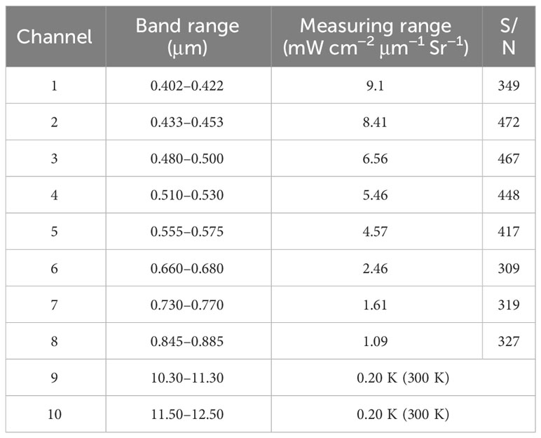
Table 1 COCTS Spectral Characteristics.

2.1.2 ERA5 data

The sea surface and atmospheric profile parameters are derived from the ERA5 data, which is the hourly global atmospheric, land, and ocean reanalysis data provided by the European Centre for Medium-Range Weather Forecasts (ECMWF). The sea surface parameters used in this algorithm include sea surface skin temperature (SST_skin), total cloud cover, sea ice fraction, and total column water vapor (TCWV). The atmospheric profile parameters include the atmospheric temperature, specific humidity, and ozone mass mixing ratio of 37 layers. The data format is NetCDF with a spatial resolution of 0.25° × 0.25° (Hersbach et al., 2020).

2.1.3 OSTIA data

The UK Met Office (UKMO) OSTIA system developed the OSTIA data using satellite data (infrared and microwave SST) and in situ SST to generate global high-resolution SST products (Donlon et al., 2012). OSTIA SST is the foundation SST. The data includes sea ice fraction data from the European Operational Satellite Agency for monitoring weather, climate, and the environment (EUMETSAT) Ocean and Sea Ice Satellite Applications Facility (OSI-SAF) (Donlon et al., 2012). The OSTIA data format is NetCDF, and the spatial resolution is 0.05° × 0.05°.

2.1.4 In situ SST

The in situ SST adopts the in situ SST quality monitor (iQuam) data, processed and distributed by the National Oceanic and Atmospheric Administration National Environmental Satellite, Data, and Information Service Satellite Applications and Research (NOAA NESDIS STAR). iQuam data include geolocation, time, and platform information. Platform types include ship, drifter, mooring, Argo, high-resolution drifter, integrated marine observing system, and coral reef buoy data (Xu and Ignatov, 2014). The quality level information is also stored in the iQuam data, pixels with a level of 5 have the highest quality, and the data format is NetCDF.

2.1.5 NOAA-20/VIIRS L1B data

The NOAA-20 VIIRS L1B data are downloaded from the Level-1 and Atmosphere Archive and Distribution System Distributed Active Archive Center (LAADS DAAC). The orbital altitude of the NOAA-20 is 834 km, and the local time when NOAA-20 crosses the equator is 1.30 pm. The nadir resolution of VIIRS is 750 km, the swath width is 3000 km, and the channels 12, 15, and 16 of VIIRS are 3.7 μm, 11 μm, and 12 μm channels, respectively (Wang and Cao, 2021). The data format is NetCDF. The NOAA-20/VIIRS BT has excellent stability, and compared with co-located Cross-track Infrared Sounder observations, the daily bias is less than 0.1 K at the nadir (Wang and Cao, 2021).

2.1.6 NOAA-20/VIIRS L2P SST

The NOAA-20 VIIRS L2P SST used in this paper is from the ACSPO system and it is provided by the NOAA National Centers for Environmental Information (NCEI). The biases of the ACSPO VIIRS SST from the buoy during the day and night are close to 0, and the standard deviations are less than 0.5°C (Petrenko et al., 2014). The validation results of the ACSPO VIIRS SST show that it can be used for the evaluation of the COCTS SST in this study. The data format of VIIRS L2P SST is NetCDF.

2.2 Selection of representative profiles

The sea surface and atmospheric parameters are used to obtain the simulated BT through the radiative transfer modeling, and the NLSST algorithm is used to fit the retrieval coefficients. The representativeness of the atmospheric profiles is crucial to obtaining a high-precision SST retrieval algorithm. The representativeness refers to the large difference in atmospheric profiles, including the atmospheric temperature, specific humidity, and ozone mass mixing ratio difference of the atmospheric profiles.

Figure 1 shows the selection process of atmospheric profiles. The time range used for selection is 0:00, 6:00, 12:00, and 18:00 on the 1st and 15th of each month in 2020. First, the initial selection of atmospheric profiles is conducted. Since the spatial resolution of ERA5 data is 0.25° × 0.25°, the spatially adjacent atmospheric profiles might have high consistency; therefore, points are taken at 1° intervals in the latitude and longitude directions. The land, ice, and cloud pixels are removed according to the ERA5 land–sea–mask, sea ice fraction, and total cloud cover. Then, the atmospheric profiles obtained from the initial selection were sampled using the Update Thermodynamic Initial Guess Retrieval (TIGR) method (Chevallier et al., 2000). The Update TIGR method selects profiles by judging the atmospheric temperature, specific humidity, and ozone mass mixing ratio differences of the profiles. If the atmospheric temperature, specific humidity, and ozone mass mixing ratio of the profile significantly differ from the selected profiles, the profile is retained. The threshold setting of the Update TIGR algorithm determines the number of selected profiles. Sampling is performed at different water vapor ranges to ensure that the water vapor range of the profiles is large, and that every 10 kg/m² is a range. Profiles of each range are combined and later used in the SST retrieval algorithm.

FIGURE 1

Figure 1 The selection process of atmospheric profiles.

The MODerate-resolution atmospheric TRANsmission (MODTRAN) is used for atmospheric radiative transfer simulation. MODTRAN is an atmospheric radiative transfer simulation calculation program. MODTRAN is widely used by scientists from governments, educational institutions, and commercial companies for optical analysis through the atmosphere. MODTRAN is used for data processing of sensors, in particular for the removal of atmospheric effects. The spectral range that can be covered by MODTARN calculation ranges from ultraviolet to long-wave infrared (0-50,000 cm^-1). Radiation transport (RT) in MODTRAN provides accurate and fast methods for modeling stratified and uniform atmospheres. The core of MODTRAN RT is the atmospheric “narrow-band model” algorithm. The atmosphere is modelled through vertical profiles, either using built-in models or by the users’ specifications. MODTRAN solves the radiative transfer equation, including absorption, emission, and scattering of atmospheric molecules, surface reflection and emission, solar or lunar illumination (Berk et al., 2008). The atmospheric profiles include temperature, humidity, pressure, ozone mass mixing ratio, SST, sea surface emissivity, and spectral response function (Berk et al., 2013). Furthermore, the aerosol and cloud parameters and the geometric relationship between the sensor and the ground must be set. MODTRAN can output information such as total radiance, BT, and transmittance. MODTRAN is one of the most accurate atmospheric RT models, with transmittance accuracy of ±0.005, radiance accuracy of ±2%, and thermal BT accuracy better than 1 K (Berk et al., 2008).

Figure 1 shows that the selected ERA5 data are used with the sensor spectral response function, satellite zenith angle, and other information to simulate the BT using the MODTRAN, and the satellite zenith angles used for the simulation are set in 5° intervals from 0° to 50°. The simulated BTs of 11 μm and 12 μm channels are obtained and used for coefficients fitting of the SST retrieval algorithm.

Figure 2 shows the spatial distribution of the profiles with values of SST_skin and BT difference. In general, the spatial distributions of the profiles are uniform, the distribution near the equator is less affected by cloud coverage, and the land edge is densely distributed due to significant changes in atmospheric conditions. Table 2 shows the number of the profiles of each water vapor range. The ratio of the after-final selection to the initial selection is calculated. The ratios of 0–10 kg/m², 10–20 kg/m², 20–30 kg/m², and 30–40 kg/m² water vapor ranges are 4.39%, 4.30%, 3.21%, and 6.38%, respectively, and are closer. The ratio of more than 40 kg/m² is larger, caused by the loose setting of the threshold for high water vapor to obtain more high water vapor in the atmospheric profiles.

FIGURE 2

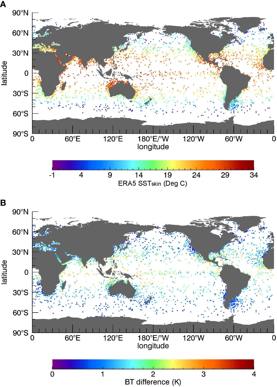
Figure 2 The spatial distribution of the profiles with values of SST_skin and BT difference (A) The color represents the ERA5 SST_skin (B) The color represents the BT difference with the satellite zenith angle of 0.

TABLE 2

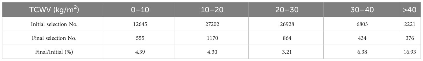
Table 2 The number of the profiles of each water vapor range.

Figure 3 shows the frequency histogram distribution of the simulated BT difference of the selected profiles when the satellite zenith angle is 0°–50°. The selected profiles are used for the coefficients fitting of the SST algorithm.

FIGURE 3

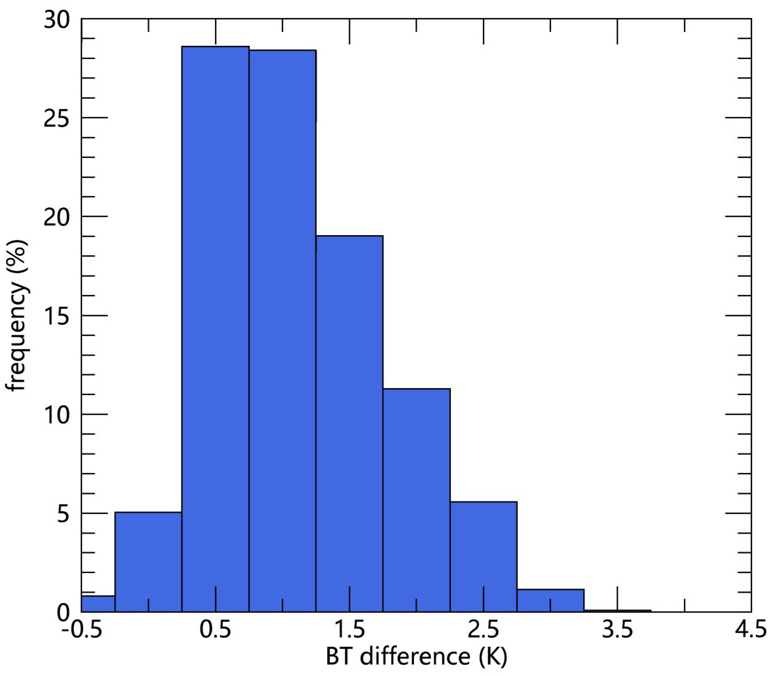
Figure 3 The frequency histogram distribution of the simulated BT difference of the selected profiles when the satellite zenith angle is 0°–50°.

2.3 SST retrieval algorithm

Based on the simulated BT for the satellite zenith angle in 0°–50° and the ERA5 SST_skin, the coefficients of the SST retrieval algorithm are obtained. In total, 37,389 points are used for the fitting and validation of the algorithm. The coefficients are fitted at different latitude bands. The latitude bands are set as 90°S–60°S, 60°S–40°S, 40°S–20°S, 20°S–0, 0–20°N, 20°N–40°N, 40°N–60°N, 60°N–90°N. The algorithm is shown in (1) (Walton et al., 1998),

$\begin{array}{ll}\begin{array}{c}SST=a_{1}B{T}_{11}+a_2{T}_{sfc}(B{T}_{11}-B{T}_{12})+\\ a_3(B{T}_{11}-B{T}_{12})\left(sec{\theta }_v-1\right)+a_4\end{array}& (1)\end{array}$

where SST is the retrieved SST, T_sfc is the estimated value of SST, BT₁₁ and BT₁₂ are 11 μm and 12 μm channel BTs, θ_v is the satellite zenith angle, and a₁–a₄ are the coefficients of the SST retrieval algorithm.

When fitting, SST in (1) uses ERA5 SST_skin, BT_11, and BT₁₂ are the corresponding simulated BT of the profiles, MCSST is used for the T_sfc. The MCSST form adopted in this study is as formula (2).

$\begin{array}{ll}\begin{array}{c}MCSST=b_{1}B{T}_{11}+b_2(B{T}_{11}-B{T}_{12})+\\ b_3(B{T}_{11}-B{T}_{12})\left(sec{\theta }_v-1\right)+b_4\end{array}& (2)\end{array}$

b₁–b₄ is the coefficients of MCSST, which are obtained by fitting ERA5 SST_skin and simulated BT. The simulated BT is added with 0.2 K Gaussian noise to be closer to the actual situation; thus, 2/3 of the data are used for fitting, and 1/3 of the data are used for validation. Figure 4 shows the relationship between ERA5 SST_skin and the 11 μm channel BT for the fitting dataset. Table 3 shows the coefficients of the SST retrieval algorithm. The validation dataset SST is obtained using the retrieval algorithm coefficients, the SST is compared with the ERA5 SST_skin, the bias is close to 0, and the standard deviation is 0.42°C. Table 4 shows the bias of the validation dataset between the calculated SST and the ERA5 SST_skin at each latitude band. The bias of each latitude band is close to 0, the standard deviation is between 0.28°C and 0.52°C, the standard deviation is the largest at 0–20°N, and the standard deviation is the smallest at 90°S–40°S. Figure 5 is the relationship between the calculated SST minus ERA5 SST_skin and ERA5 SST_skin. The color represents the number of matchups in the squares. The red and black lines represent the bias and standard deviation of a specific SST range, respectively. The bias has no apparent relationship with the SST_skin value. Figure 6 shows the relationship between the calculated SST minus ERA5 SST_skin and the simulated BT difference. The standard deviation increases with the increasing BT difference, but the maximum value is approximately 0.5°C. In summary, the algorithm has good performance and can be used for SST retrieval.

FIGURE 4

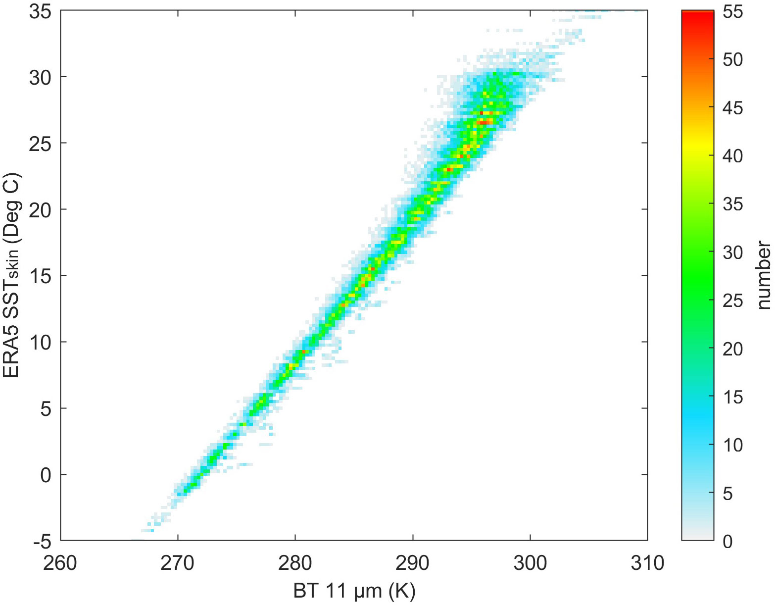
Figure 4 The relationship between ERA5 SST_skin and the 11 μm channel BT.

TABLE 3

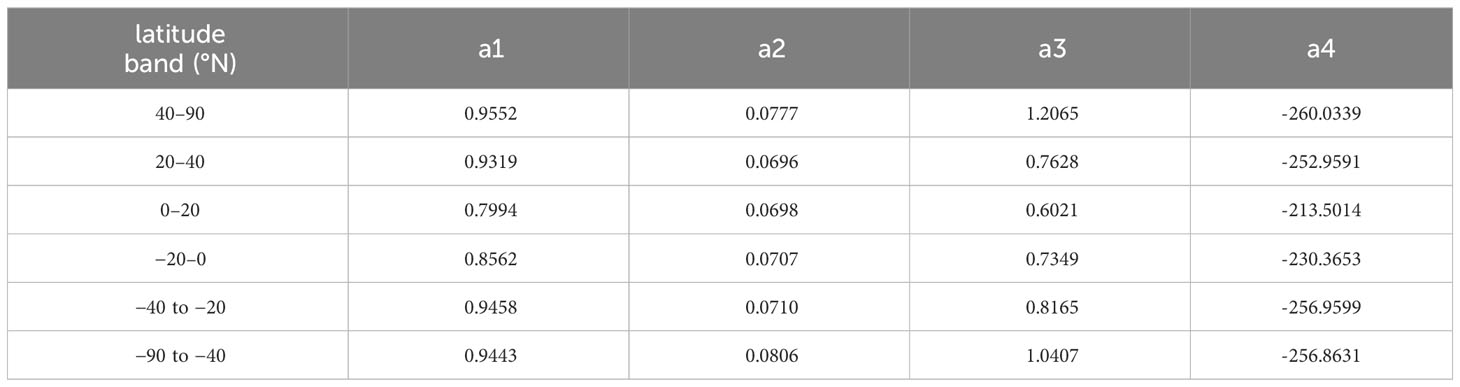
Table 3 The coefficients of the SST retrieval algorithm.

TABLE 4

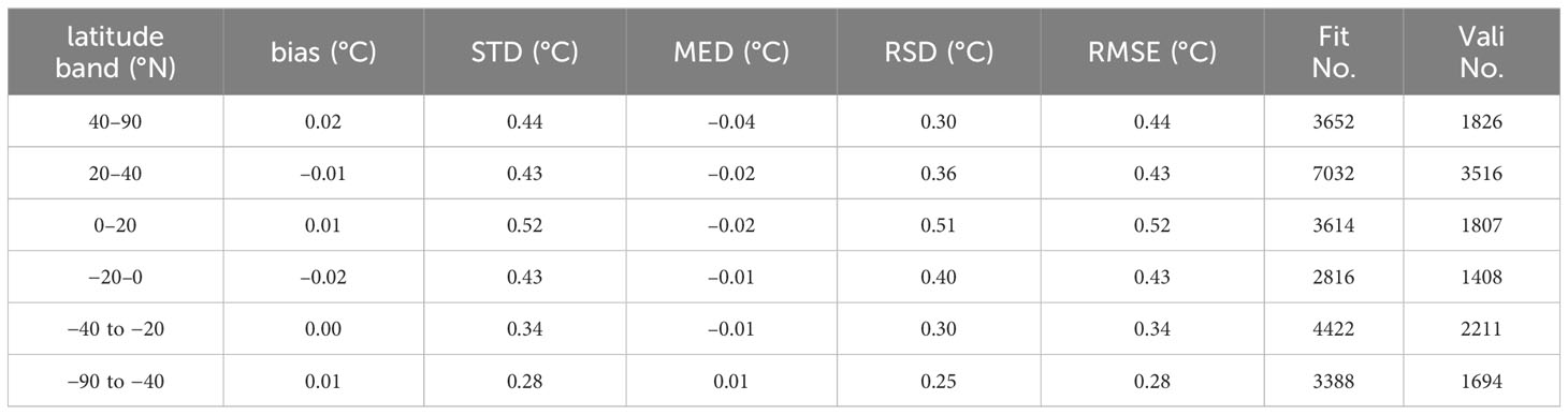
Table 4 The bias of the validation dataset between the calculated SST and the ERA5 SST_skin at each latitude band [standard deviation (STD), median (MED), robust standard deviation (RSD)].

FIGURE 5

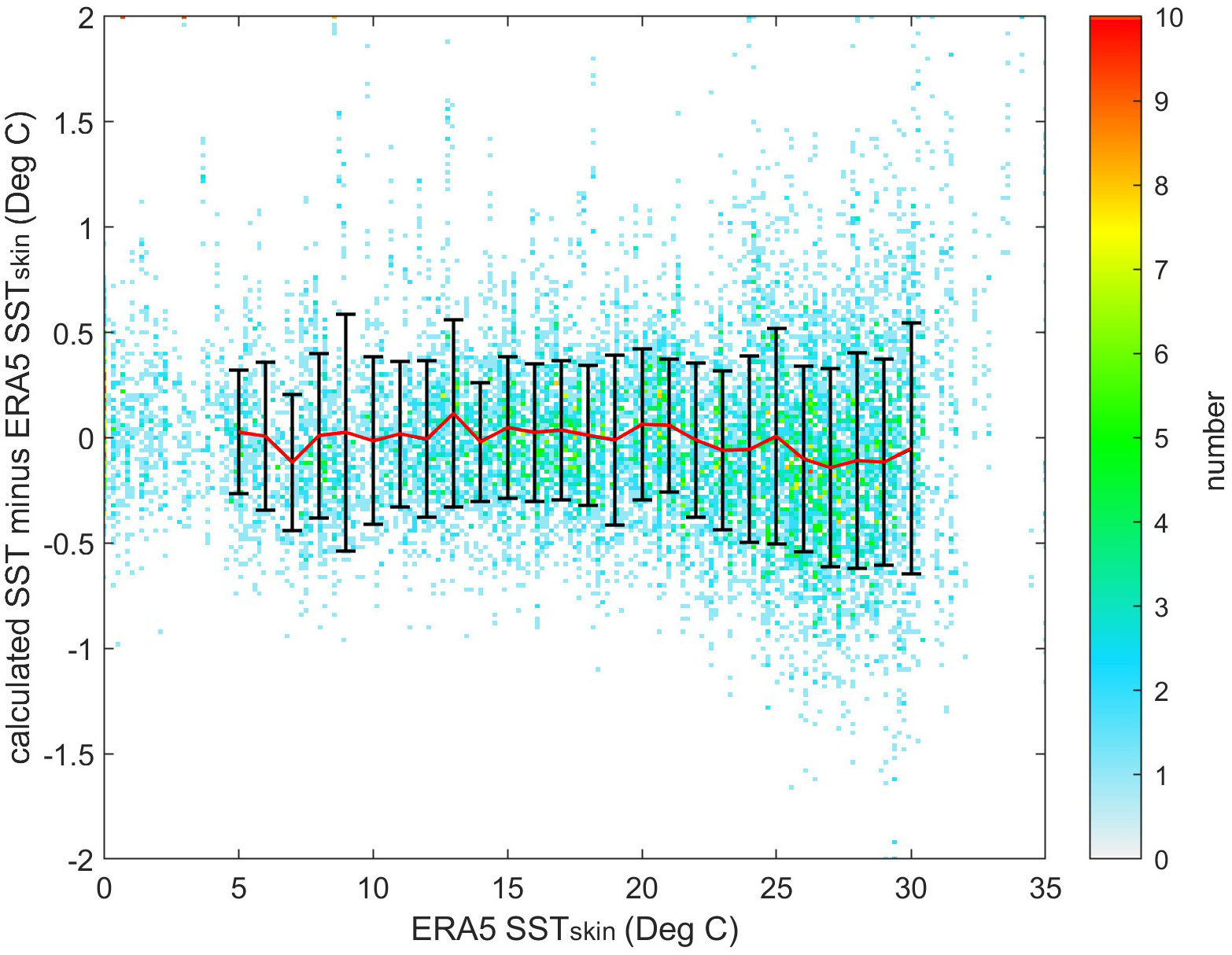
Figure 5 The relationship between the calculated SST minus ERA5 SST_skin and ERA5 SST_skin.

FIGURE 6

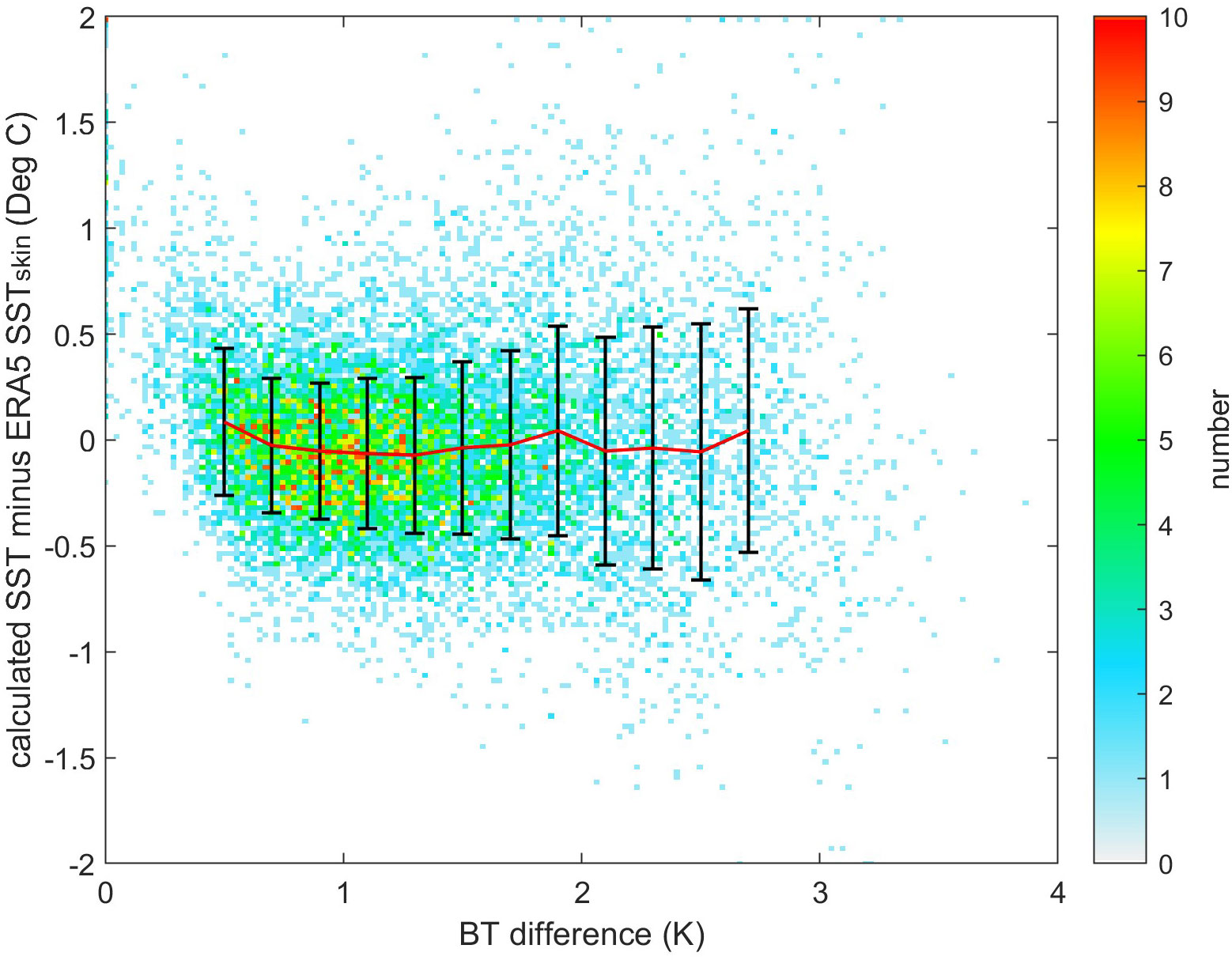
Figure 6 The relationship between the calculated SST minus ERA5 SST_skin and the simulated BT difference.

The COCTS BT inter-calibrated with VIIRS is used for SST retrieval, the bias between inter-calibrated COCTS BT and VIIRS BT is about 0, and the standard deviation is about 0.1°C. The latitude interval of the pixel is first judged, and the SST retrieval algorithm corresponding to the latitude interval is used for retrieval. The weighted average of the SSTs of two adjacent latitude bands is used within 2.5° of the latitude boundary to reduce the discontinuity at the edge of the latitude band. The estimated value of SST applies to OSTIA SST.

2.4 Cloud detection

The threshold method is used for cloud detection. The data include 670 nm and 865 nm channel reflectance, 11 μm and 12 μm channel BT, the solar zenith angle, OSTIA data, and the obtained COCTS SST. The OSTIA SST in the OSTIA data is used as the reference SST for cloud detection, and the sea ice fraction is used for ice pixel removal before cloud detection. Cloud pixels have low BT values, large BT differences between the channels, poor uniformity, and large negative bias from the reference SST. Therefore, the BT values of the 11 μm and 12 μm channels, the BT differences of the 11 μm and 12 μm channels, BT uniformity, COCTS SST, and reference SST differences are used as cloud detection parameters. Cloud pixels have high reflectance; therefore, the reflectance and reflectance ratio of the visible channels are selected as the cloud detection parameters during the day. First, the cloud is identified according to the BT value and BT difference between the 11 μm and 12 μm channels and the uniformity of the 11 μm channel BT. Then, the daytime and nighttime judgments are performed according to the solar zenith angle. If it is daytime, cloud detection is performed according to the reflectance of the visible channels, and the difference between the COCTS SST and the reference SST is judged. If it is nighttime, the difference between the COCTS SST and the reference SST is judged. Figure 7 shows the cloud detection process, which is as follows.

1. Determine whether the 11 μm or 12 μm channel BT is greater than 260 K. If they are less than or equal to 260 K, it is determined as a cloud pixel.

2. Determine whether the difference between the 11 μm and 12 μm channel BT is less than 4 K, and if it is greater than or equal to 4 K, it is determined as a cloud pixel.

3. Determine whether the standard deviation of the difference between the 11 μm channel BT and the median of the 11 μm channel BT in the 3 × 3 area pixels is less than 0.3 K. If it is greater than or equal to 0.3 K, it is determined as a cloud pixel. Compared with the standard deviation of the 11 μm channel BT in the 3 × 3 area, the method can effectively reduce the over-detection of clouds at the front (Petrenko et al., 2010).

4. Determine daytime and nighttime according to the solar zenith angle. If the solar zenith angle is less than 85°, it is determined as a daytime pixel, and if it is greater than or equal to 85°, it is determined as a nighttime pixel.

5. In the daytime, determine whether the 865 nm channel reflectance is less than the threshold η1. Then determine whether the 865 nm channel reflectance to the 665 nm channel reflectance ratio is less than the threshold η1. It is determined to be cloud pixels if it is greater than or equal to the threshold. The thresholds here are all set as dynamic thresholds, and the thresholds of the glint areas are larger than other areas (Petrenko et al., 2010). Determine whether the difference between the COCTS SST and the reference SST is greater than −1.2°C, and if it is less than −1.2°C, it is determined as a cloud pixel.

6. In the nighttime, determine whether the difference between the COCTS SST and the reference SST is greater than −1.2°C, and if it is less than −1.2°C, it is determined as a cloud pixel.

FIGURE 7

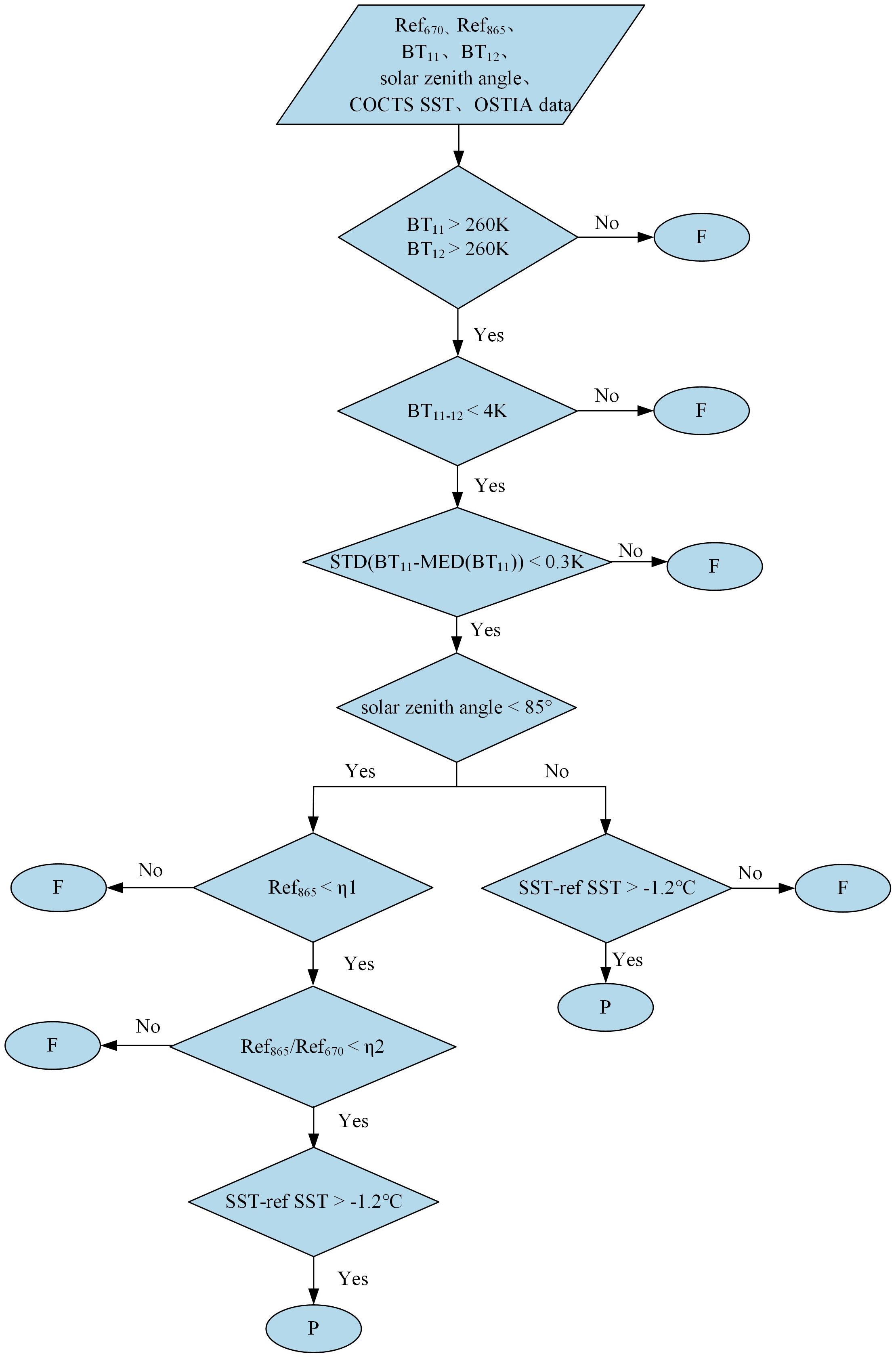
Figure 7 The cloud detection process.

Figure 8 shows the COCTS SST swaths before and after cloud detection in the daytime and nighttime. There is no obvious phenomenon of judging clear sky pixels as cloud pixels in the daytime and nighttime.

FIGURE 8

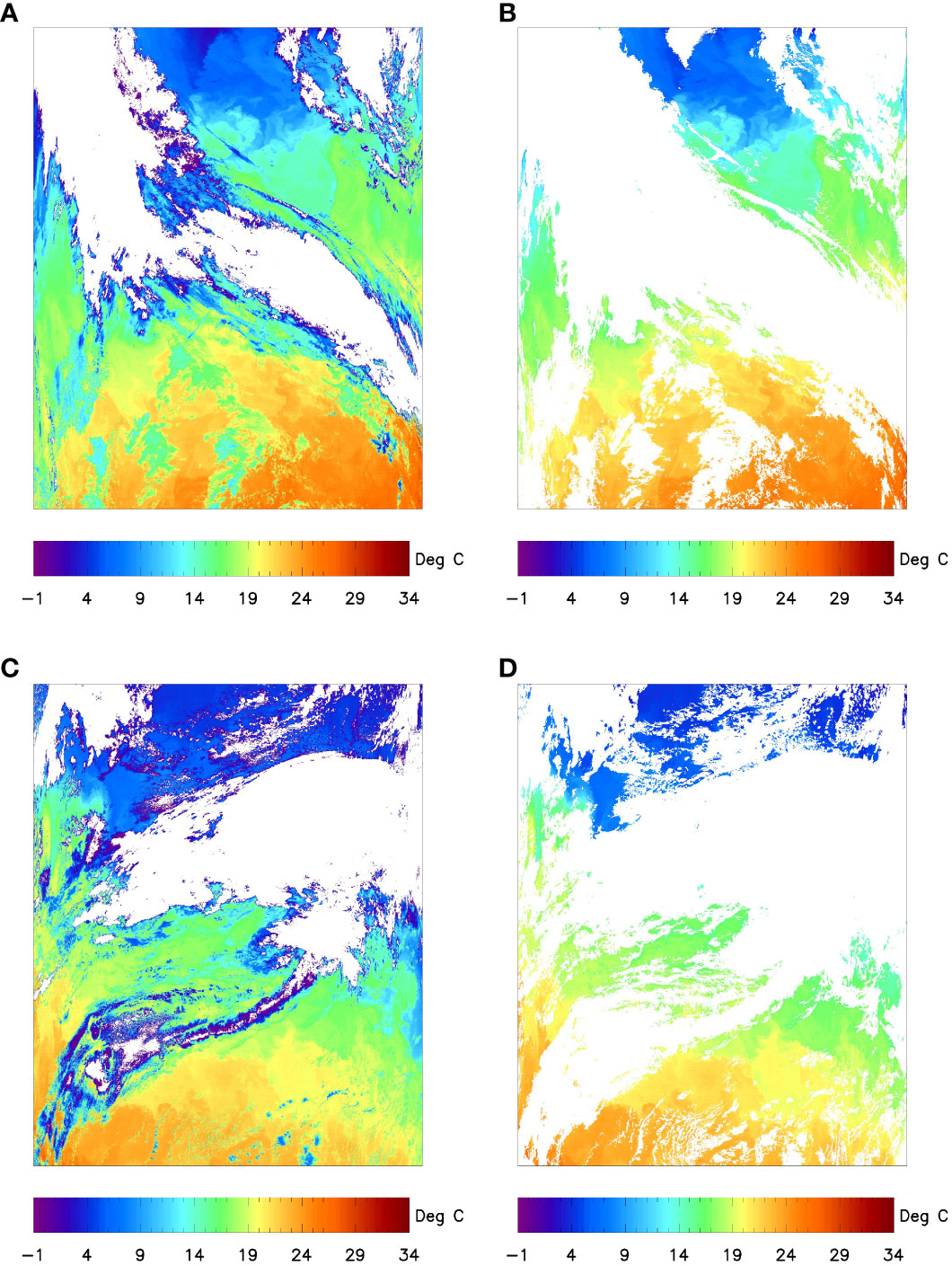
Figure 8 The COCTS SST swaths before and after cloud detection in the daytime and nighttime (A) Daytime before cloud detection on 4 May, 2021 (B) Daytime after cloud detection on 4 May, 2021 (C) Nighttime before cloud detection on 16 May, 2021. (D) Nighttime after cloud detection on 16 May, 2021.

2.5 Quality level defined

SST quality levels are available to meet the different needs of SST users. Land, ice, and clouds affect the SST quality; therefore, land and ice masks and cloud edge information are used for quality level definition. High-quality pixels should have a reasonable SST range, and their SSTs should be close to the reference SST. Therefore, the COCTS SST range and the difference between the COCTS SST and the reference SST indicate the quality level defined. The accuracy of SST validation in sea areas with poor uniformity might be affected. Simultaneously, because the noise of the SST from the retrieval is greater than that of BT, the uniformity of BT is selected as an index of the quality level defined. Atmospheric paths affect pixels with excessive satellite zenith angles, and their corresponding SST accuracy might be affected; therefore, satellite zenith angles are used as the standard for the quality level defined.

Figure 9 is the quality level map of the COCTS SST of the two granules on 4 May 2021 and 16 May 2021. The red area has a quality level of 0 (land or ice pixels), the orange area has a quality level of 1 (cloud pixels), the yellow area has a quality level of 2 (pixels whose SST or difference from the reference SST is not within a given threshold range), the light blue area has a quality level of 3 (pixels with poor BT uniformity), and a darker blue area has a quality level of 4 (pixels at the edge of clouds or with larger satellite zenith angles). The dark blue area has a quality level of 5, which are pixels with the highest quality.

FIGURE 9

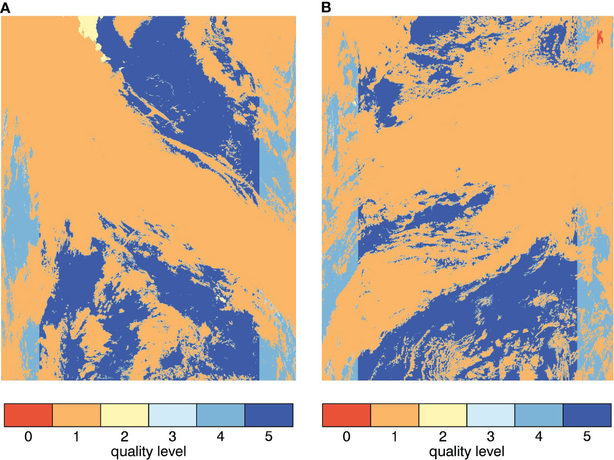
Figure 9 The quality level map of the COCTS SST swaths (A) Daytime on 4 May, 2021 (B) Nighttime on 16 May, 2021.

3 Results and discussion

The global COCTS data during the period of May to July 2021 are processed and the skin SST products are obtained. Figure 10 shows the COCTS SST in the daytime and nighttime on 1 May, 2021. The COCTS SST is evaluated using iQuam data and ACSPO VIIRS L2P SST. iQuam data is used to validate the accuracy of COCTS SST and the rationality of quality level, and the iQuam data is also used to analyze the stability of the algorithm. ACSPO VIIRS L2P SST is used to cross-validate the accuracy of COCTS SST and analyze the daily bias, and the spatial distribution characteristics of the bias are analyzed.

FIGURE 10

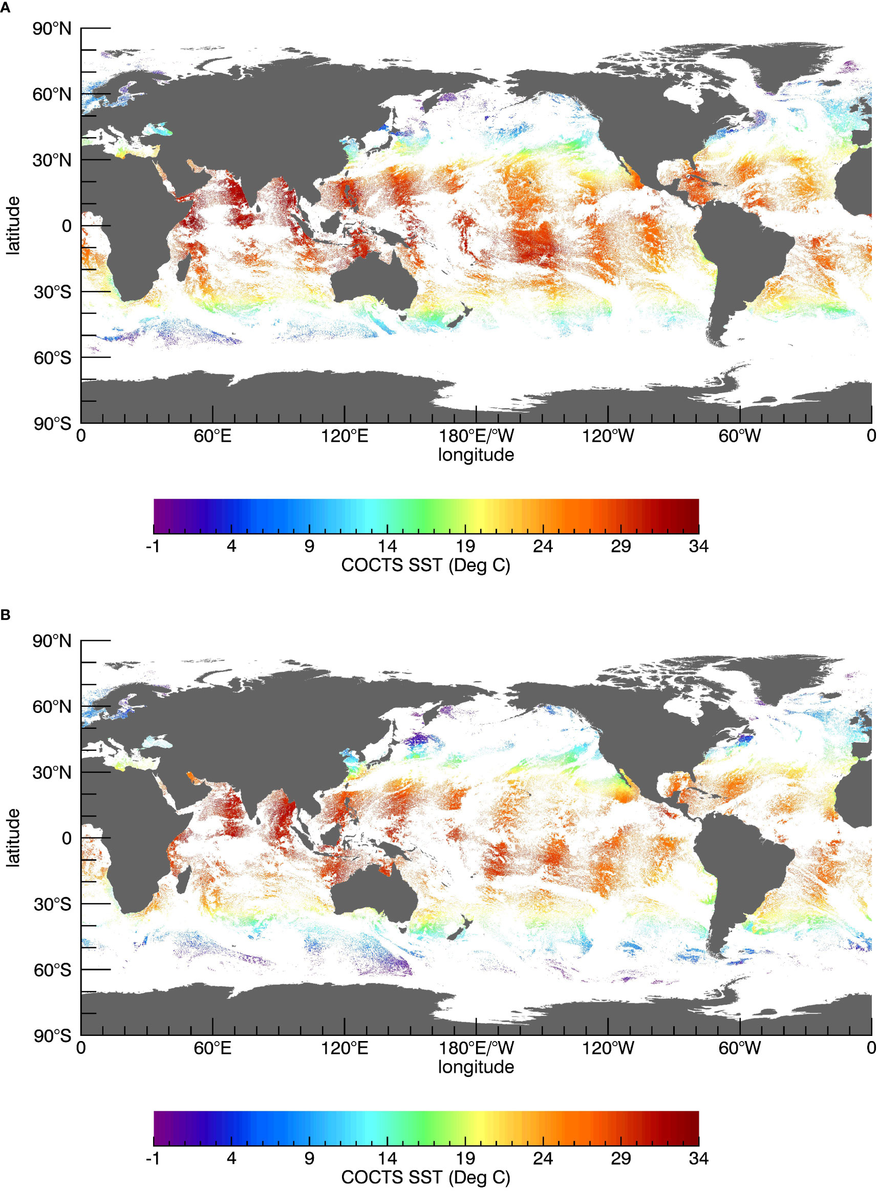
Figure 10 The COCTS SST in the daytime and nighttime on 1 May, 2021 (A) Daytime (B) Nighttime.

The COCTS SST is matched with the drifters, high-resolution drifters, tropical moorings, coastal moorings, and Argo floats with the highest quality level in the iQuam data. The time window is 1 h, and the spatial window is 0.01° × 0.01°. Pixels with quality levels of 2, 3, 4, and 5 account for 1.93%, 6.76%, 30.75%, and 60.55% of the total number of matchups. Pixels with quality levels of 4 and 5 account for 91.30% of the total number of matchups, and pixels with quality levels 3, 4, and 5 account for 98.07% of the total number of matchups. The proportion indicates the rationality of the quality level. Table 5 shows the statistical results of quality levels 3, 4, and 5. As the quality level increases, the standard deviation decreases. The standard deviation of pixels with a quality level of 3 is significant due to poor uniformity. The pixels with a quality level of 4 have small negative deviations because they are on the edge of the cloud.

TABLE 5

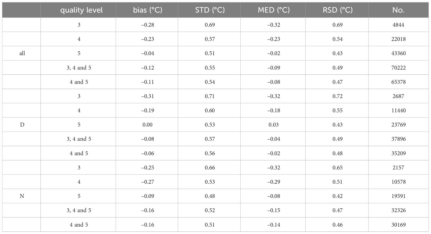
Table 5 Statistical results of the bias between the COCTS and in situ SSTs (D means daytime and N means nighttime).

There are 65,378 matchups in quality levels 4 and 5, with a bias of –0.11°C, a standard deviation of 0.54°C, a median of –0.08°C, and a robust standard deviation of 0.47°C. The bias in the daytime is –0.06°C, the standard deviation is 0.56°C, the median is –0.02°C and the robust standard deviation is 0.48°C. The bias in the nighttime is –0.16°C, the standard deviation is 0.51°C, the median is –0.14°C and the robust standard deviation is 0.46°C. There is a small negative bias due to the cool skin effect. The negative bias in the daytime is smaller than in the nighttime due to solar radiation. The standard deviation in the daytime is more significant than in the nighttime. Figure 11 shows the histogram distribution of the bias between the COCTS SST and the in situ SST. The bias between the COCTS SST and in situ SST has an obvious Gaussian distribution. Figure 12 shows the relationship between the bias of the COCTS and in situ SSTs and the in situ SST. The bias does not have a significant trend with the in situ SST. Since the BT difference between the 11 μm and 12 μm channels is related to the water vapor content, the relationship between the bias of the COCTS and in situ SSTs and the BT difference is analyzed. Figure 13 shows that the bias has no obvious relationship with the BT difference.

FIGURE 11

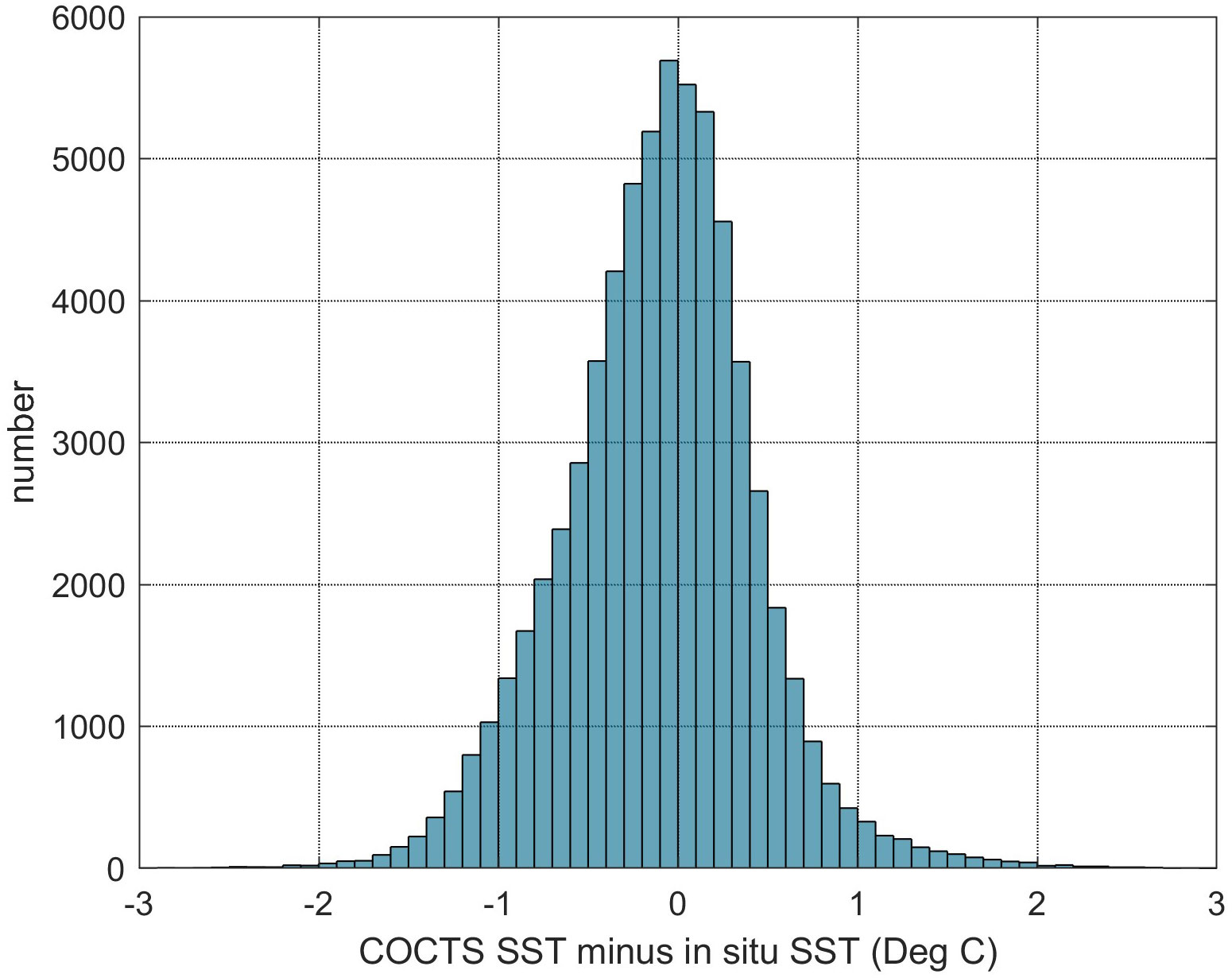
Figure 11 The histogram distribution of the bias between the COCTS SST and the in situ SST.

FIGURE 12

Figure 12 The relationship between the bias of the COCTS and in situ SSTs and the in situ SST.

FIGURE 13

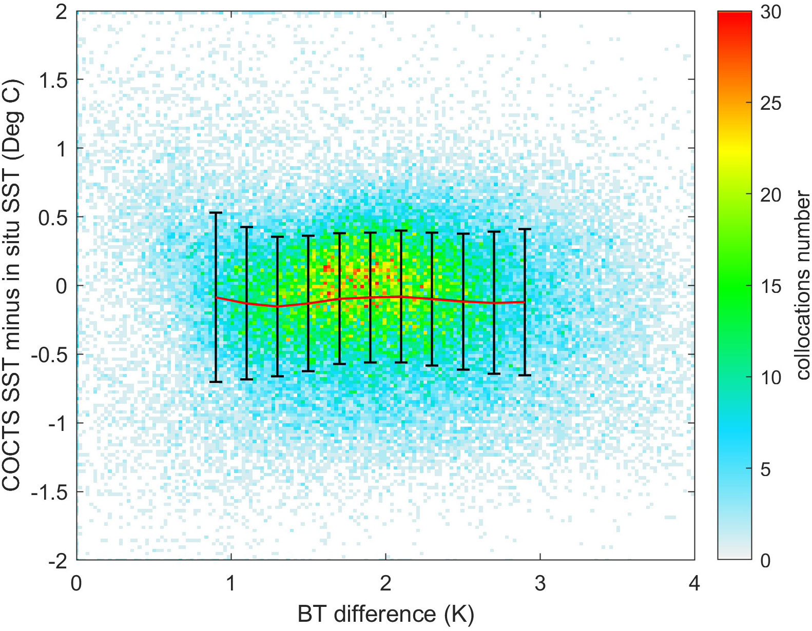
Figure 13 The relationship between the bias of the COCTS and in situ SSTs and the BT difference.

The VIIRS SST data also contains quality levels, and the pixels with the quality levels 4 and 5 have the best quality. The COCTS SST with the quality levels of 4 and 5 is compared with the VIIRS SST. The time window is 1 h, and the spatial window is 0.01° × 0.01°. Table 6 shows the statistical results. There are 4,455,678,619 matchups. The bias is 0.03°C, the standard deviation is 0.53°C, the median is 0.06°C, and the robust standard deviation is 0.49°C. The bias in the daytime is 0.12°C, the standard deviation is 0.52°C, the median is 0.15°C, and the robust standard deviation is 0.47°C. The bias in the nighttime is –0.08°C, the standard deviation is 0.51°C, the median is –0.06°C and the robust standard deviation is 0.48°C. Figure 14. shows the daily statistics of COCTS SST and VIIRS SST, where the black line represents the bias, the red line represents the standard deviation, the blue line represents the median, and the purple line represents the robust standard deviation. The biases are close to the medians, most of them are distributed between –0.1 to 0.1°C. Most of the standard deviations are distributed around 0.5°C, and the robust standard deviations are slightly smaller than the standard deviations. There is no significant change in statistical results over time. Figure 15. shows the spatial distribution of the bias of COCTS SST and VIIRS SST. It can be seen that in most areas, COCTS SST and VIIRS SST are closer. For daytime, there is a positive deviation in some areas, which may be driven by solar heating, for nighttime, there is a negative bias in some areas, which may be caused by the cool skin effects. The higher COCTS SST near land in the daytime and nighttime may be due to the inaccuracy of ERA5 SST_skin on the land edge and the inaccuracy of COCTS positioning.

TABLE 6

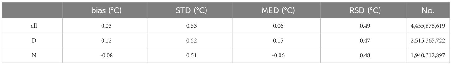
Table 6 Statistical results of the bias between the COCTS and VIIRS SSTs.

FIGURE 14

Figure 14 The daily statistics of COCTS SST and VIIRS SST.

FIGURE 15

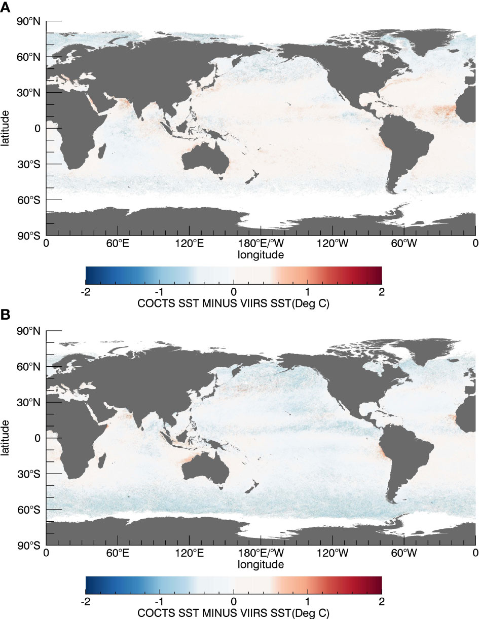
Figure 15 The spatial distribution of the bias of COCTS SST and VIIRS SST. (A) Daytime (B) Nighttime.

In addition to the influence of the diurnal variety of SST, the error sources include sensor noise, uncertainty of the observed BT calibration, atmospheric radiative transfer modeling errors, and atmospheric profile errors. Atmospheric profile and radiative transfer modeling errors directly affect the accuracy of the simulated BT, leading to bias in the relationship between the ERA5 SST_skin and the simulated BT and affecting the accuracy of the algorithm. The observed BT calibration accuracy can also lead to poor retrieval results. Simultaneously, the equivalent temperature difference of the sensor noise affects the standard deviation of the retrieval results.

4 Conclusions

The HY-1D/COCTS skin SST retrieval is performed based on atmospheric radiative transfer modeling. The representative ERA5 atmospheric profiles are selected for fitting the coefficients of the SST retrieval algorithms, and the SST retrieval algorithms of the latitude bands are obtained. The retrieval of COCTS SST is conducted using COCTS BT inter-calibrated with VIIRS, and the COCTS cloud detection is performed with the reference SST. The retrieval results are compared with the in situ SST and VIIRS SST. The bias with in situ SST is –0.11°C and the standard deviation is 0.54°C. The bias with VIIRS SST is 0.03°C, and the standard deviation is 0.53°C. Therefore, the retrieval algorithm based on atmospheric radiative transfer modeling works well in the HY-1D/COCTS SST retrieval. In the future, the algorithm will be applied for COCTS SST retrieval of long-time series.

Data availability statement

Publicly available datasets were analyzed in this study. This data can be found here: https://osdds.nsoas.org.cn/OceanColor, https://cds.climate.copernicus.eu/#!/search?text=ERA5&type=dataset, https://resources.marine.copernicus.eu/products, https://www.star.nesdis.noaa.gov/socd/sst/iquam/data.html, https://ladsweb.modaps.eosdis.nasa.gov/search/, https://www.ncei.noaa.gov/data/oceans/ghrsst/L2P/VIIRS_NPP/OSPO/.

Author contributions

ZL and LG contributed to the conception and methodology of the study. ZL organized the database. RC performed the inter-calibration. ZL wrote the first draft of the manuscript. All authors contributed to the manuscript revision, and read and approved the submitted version.

Funding

This work was supported by the National Key R&D Program of China (2022YFC3104900/2022YFC3104905), the Hainan Special PhD Scientific Research Foundation of Sanya Yazhou Bay Science and Technology City (HSPHDSRF-2022-02-001) and Hainan Provincial Natural Science Foundation of China (122CXTD519).

Acknowledgments

The authors would like to thank the National Satellite Ocean Application Service (NSOAS) for providing the COCTS L1B data. ERA5 data are provided by European Centre for Medium-Range Weather Forecasts (ECMWF), OSTIA data are from UK Met Office (UKMO), iQuam data are provided by National Oceanic and Atmospheric Administration National Environmental Satellite, Data, and Information Service Satellite Applications and Research (NOAA NESDIS STAR), the VIIRS L1B data are downloaded from Level-1 and Atmosphere Archive and Distribution System Distributed Active Archive Center (LAADS DAAC), the ACSPO VIIRS L2P SST data are provided by National Oceanic and Atmospheric Administration (NOAA) National Centers for Environmental Information (NCEI).

Conflict of interest

The authors declare that the research was conducted in the absence of any commercial or financial relationships that could be construed as a potential conflict of interest.

Publisher’s note

All claims expressed in this article are solely those of the authors and do not necessarily represent those of their affiliated organizations, or those of the publisher, the editors and the reviewers. Any product that may be evaluated in this article, or claim that may be made by its manufacturer, is not guaranteed or endorsed by the publisher.

References

Aydoğdu A., Pinardi N., Pistoia J., Martinelli M., Belardinelli A., Sparnocchia S. (2016). Assimilation experiments for the fishery observing system in the Adriatic Sea. J. Mar. Syst. 162, 126–136. doi: 10.1016/j.jmarsys.2016.03.002

CrossRef Full Text | Google Scholar

Barnett T. P., Graham N., Pazan S., White W., Latif M., Flügel M. (1993). ENSO and ENSO-related predictability. Part I: Prediction of equatorial Pacific sea surface temperature with a hybrid coupled ocean–atmosphere model. J. Climate 6 (8), 1545–1566. doi: 10.1175/1520-0442(1993)006<1545:EAERPP>2.0.CO;2

CrossRef Full Text | Google Scholar

Berk A., Acharya P. K., Bernstein L. S., Anderson G. P., Lewis P., Chetwynd J. H., et al. (2008). Band model method for modeling atmospheric propagation at arbitrarily fine spectral resolution. U.S. Patent No. 7,433,806. 7 Oct. 2008. (Washington, US: U.S. Patent and Trademark Office).

Google Scholar

Berk A., Anderson G. P., Acharya P. K. (2013). MODTRAN 5.3.2 USER’S MANUAL. US: Spectral Sciences, Inc.

Google Scholar

Chevallier F., Chédin A., Chéruy F., Morcrette J. J. (2000). TIGR-like atmospheric-profile databases for accurate radiative-flux computation. Q. J. R. Meteorol. Soc. 126 (563), 777–785. doi: 10.1002/qj.49712656319

CrossRef Full Text | Google Scholar

Dai A. (2016). Future warming patterns linked to today’s climate variability. Sci. Rep. 6 (1), 1–6. doi: 10.1038/srep19110

PubMed Abstract | CrossRef Full Text | Google Scholar

Donlon C. J., Martin M., Stark J., Roberts-Jones J., Fiedler E., Wimmer W. (2012). The operational sea surface temperature and sea ice analysis (OSTIA) system. Remote Sens. Environ. 116, 140–158. doi: 10.1016/j.rse.2010.10.017

CrossRef Full Text | Google Scholar

Hersbach H., Bell B., Berrisford P., Hirahara S., Horányi A., Muñoz-Sabater J. (2020). The ERA5 global reanalysis. Q. J. R. Meteorol. Soc. 146 (730), 1999–2049. doi: 10.1002/qj.3803

CrossRef Full Text | Google Scholar

Kilpatrick K. A., Podestá G. P., Evans R. (2001). Overview of the NOAA/NASA advanced very high resolution radiometer Pathfinder algorithm for sea surface temperature and associated matchup database. J. Geophys. Res.: Oceans 106 (C5), 9179–9197. doi: 10.1029/1999JC000065

CrossRef Full Text | Google Scholar

Kilpatrick K. A., Podestá G., Walsh S., Williams E., Halliwell V., Szczodrak M. (2015). A decade of sea surface temperature from MODIS. Remote Sens. Environ. 165, 27–41. doi: 10.1016/j.rse.2015.04.023

CrossRef Full Text | Google Scholar

Li Z., Liu M., Wang S., Qu L., Guan L. (2022). Sea surface skin temperature retrieval from FY-3C/VIRR. Remote Sens. 14 (6), 1451. doi: 10.3390/rs14061451

CrossRef Full Text | Google Scholar

Liu M., Merchant C. J., Embury O., Liu J., Song Q., Guan L. (2022). Retrieval of sea surface temperature from HY-1B COCTS. IEEE Trans. Geosci. Remote Sens. 60, 1–13. doi: 10.1109/TGRS.2022.3190444

CrossRef Full Text | Google Scholar

Llewellyn-Jones D. T., Minnett P. J., Saunders R. W., Závody A. M. (1984). Satellite multichannel infrared measurements of sea surface temperature of the NE Atlantic Ocean using AVHRR/2. Q. J. R. Meteorol. Soc. 110 (465), 613–631. doi: 10.1002/qj.49711046504

CrossRef Full Text | Google Scholar

Luo B., Minnett P. J., Szczodrak M., Kilpatrick K., Izaguirre M. (2020). Validation of Sentinel-3A SLSTR derived Sea-Surface Skin Temperatures with those of the shipborne M-AERI. Remote Sens. Environ. 244, 111826. doi: 10.1016/j.rse.2020.111826

CrossRef Full Text | Google Scholar

McClain E. P., Pichel W. G., Walton C. C. (1985). Comparative performance of AVHRR-based multichannel sea surface temperatures. J. Geophys. Res.: Oceans 90 (C6), 11587–11601. doi: 10.1029/JC090iC06p11587

CrossRef Full Text | Google Scholar

Merchant C. (2012). Sea Surface Temperature (SLSTR) Algorithm Theoretical Basis Document. (Edinburgh: University of Edinburgh).

Google Scholar

Merchant C. J., Le Borgne P., Marsouin A., Roquet H. (2008). Optimal estimation of sea surface temperature from split-window observations. Remote Sens. Environ. 112 (5), 2469–2484. doi: 10.1016/j.rse.2007.11.011

CrossRef Full Text | Google Scholar

Petrenko B., Ignatov A., Kihai Y., Heidinger A. (2010). Clear-sky mask for the advanced clear-sky processor for oceans. J. Atmos. Oceanic Technol. 27 (10), 1609–1623. doi: 10.1175/2010JTECHA1413.1

CrossRef Full Text | Google Scholar

Petrenko B., Ignatov A., Kihai Y., Stroup J., Dash P. (2014). Evaluation and selection of SST regression algorithms for JPSS VIIRS. J. Geophys. Res.: Atmospheres 119 (8), 4580–4599. doi: 10.1002/2013JD020637

CrossRef Full Text | Google Scholar

Walton C. C., Pichel W. G., Sapper J. F., May D. A. (1998). The development and operational application of nonlinear algorithms for the measurement of sea surface temperatures with the NOAA polar-orbiting environmental satellites. J. Geophys. Res.: Oceans 103 (C12), 27999–28012. doi: 10.1029/98JC02370

CrossRef Full Text | Google Scholar

Wang W., Cao C. (2021). NOAA-20 and S-NPP VIIRS thermal emissive bands on-orbit calibration algorithm update and long-term performance inter-comparison. Remote Sens. 13 (3), 448. doi: 10.3390/rs13030448

CrossRef Full Text | Google Scholar

Wang S. J., Cui P., Zhang P., Yang Z. D., Ran M. N., Xiu-Qing H. U., et al. (2017). Progress of VIRR sea surface temperature product of FY-3 satellite. Aerosp. Shanghai 34, 79–84. doi: 10.19328/j.cnki.1006-1630.2017.04.010

CrossRef Full Text | Google Scholar

Wang Q., Jing Z., Sun C. (2003). Sea surface temperature retrieval using the HY-1 satellite data. Mar. Forecasts 20 (3), 7.

Google Scholar

Ward M. N., Folland C. K. (1991). Prediction of seasonal rainfall in the north nordeste of Brazil using eigenvectors of sea-surface temperature. Int. J. Climatol. 11 (7), 711–743. doi: 10.1002/joc.3370110703

CrossRef Full Text | Google Scholar

Xu F., Ignatov A. (2014). In situ SST quality monitor (iQuam). J. Atmos. Oceanic Technol. 31 (1), 164–180. doi: 10.1175/JTECH-D-13-00121.1

CrossRef Full Text | Google Scholar

Ye X., Liu J., Lin M., Ding J., Zou B., Song Q. (2020). Sea surface temperatures derived from COCTS onboard the HY-1C satellite. IEEE J. Selected Topics Appl. Earth Observ. Remote Sens. 14, 1038–1047. doi: 10.1109/JSTARS.2020.3033317

CrossRef Full Text | Google Scholar

Ye X., Liu J., Lin M., Ding J., Zou B., Song Q., et al. (2021). Evaluation of sea surface temperatures derived from the HY-1D satellite. IEEE J. Selected Topics Appl. Earth Observ. Remote Sens. 15, 654–665. doi: 10.1109/JSTARS.2021.3137230

CrossRef Full Text | Google Scholar

Závody A. M., Mutlow C. T., Llewellyn-Jones D. T. (1995). A radiative transfer model for sea surface temperature retrieval for the along-track scanning radiometer. J. Geophys. Res.: Oceans 100 (C1), 937–952. doi: 10.1029/94JC02170

CrossRef Full Text | Google Scholar