CFD-DEM modeling of turbidity current propagation in channels with two different topographic configurations

1 Introduction

Submarine turbidity currents are a type of underwater density flow that can carry a huge amount of sediment and move downward along continental slopes or submarine canyons to deep-sea areas, which are generally recognized as one of the world’s most significant processes of sediment transport (Meiburg and Kneller, 2010; Talling, 2013; Kneller et al., 2016; Liu et al., 2022). Turbidites, regarded as the product of turbidity current deposition, are an important class of hydrocarbon reservoirs. Additionally, turbidity currents have attracted intensive concern due to their characterization of high flow velocities and extremely destructive impacts, bringing potential threats to subsea facilities (Krause et al., 1970; Hsu et al., 2008). A typical process of turbidity current generation is often related to the slope failure events, in which the post-failure soil mass is diluted due to seawater entrainment and further evolves into debris flow with high sediment concentration, and subsequently into turbidity current with low sediment concentration (Guo et al., 2023a; Liu et al., 2023), as indicated in Figure 1. Many uncertainties are included in this process, for instance the hydrodynamic conditions, seabed topographies and changes of sediment-seawater mixture properties, making it difficult to investigate the turbidity current dynamics and constraining the prediction of seaward sediment transport.

FIGURE 1

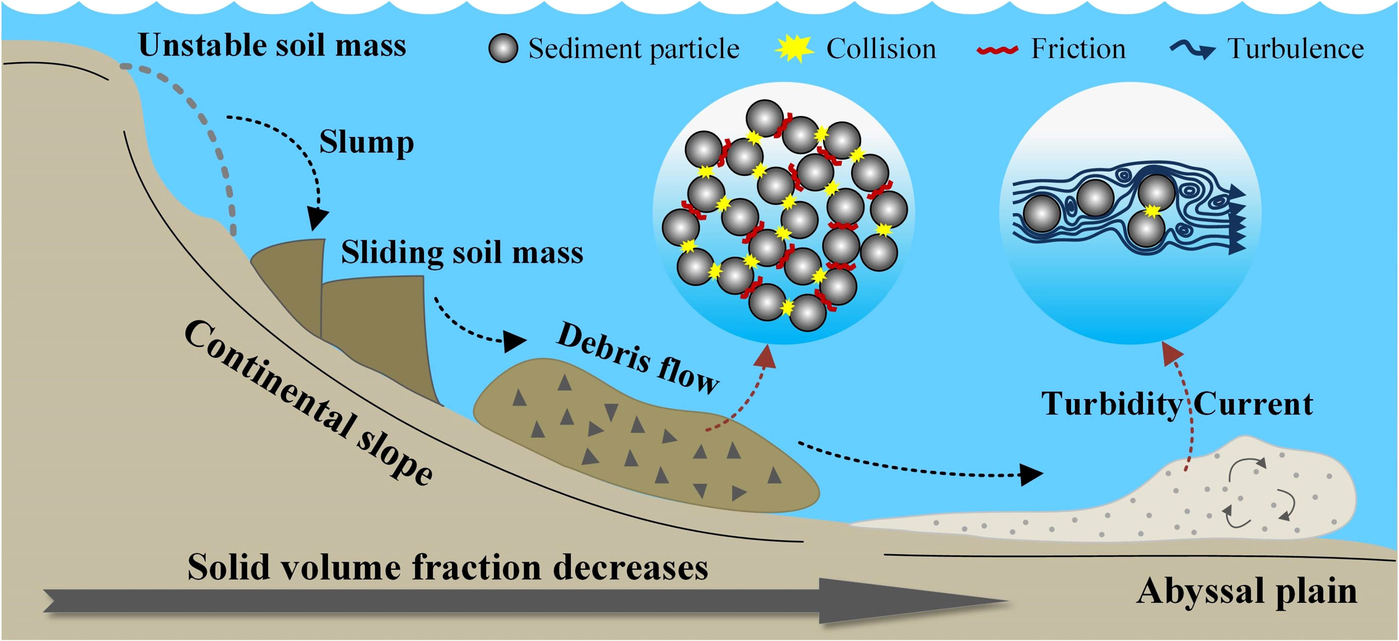
Figure 1 Schematic diagram of transformation process form unstable soil mass to turbidity current [modified from Lube et al. (2020)].

In recent years, the comprehensive understanding of turbidity current dynamics has been greatly promoted, which is benefited from the gradually improved techniques of field observations and measurements. However, high costs and difficult operating conditions result in relatively scarce studies of field observations. To date, the detailed understanding of turbidity current dynamics is still highly reliant on outcrop studies (Plink-Björklund and Steel, 2004; Li et al., 2016), scaled laboratory tests (de Leeuw et al., 2018; Pohl et al., 2019) and numerical simulations (Huang et al., 2008; Lucchese et al., 2019). Among these research methods, a validated numerical model has a distinct feature of being capable of modeling sediment transport in various scales corresponding to multi-scale processes encountered in environmental fluid dynamics (Vowinckel, 2021). The macroscale modeling using the continuum models of coupled transport equations can resolve the sediment dynamics in field scales of several tens of kilometers (Aas et al., 2010; Howlett et al., 2019). Several studies have put a lot of effort into the response of turbidity currents to the ideal or real topographies of normal faults, relay ramps, cyclic steps, and submarine canyons, using the continuum models with ignoring the particle contact behaviors (Abd El-Gawad et al., 2012; Ge et al., 2017; Ge et al., 2018; Vellinga et al., 2018). As pointed out by Biegert et al. (2017), the traditional continuum-based models are severely restricted in modeling the complex flow behaviors in the near-bed region with a high sediment concentration, where the inter-particle interactions cannot be neglected. Therefore, a discrete element method (DEM) might be more appropriate, which treats the turbidity currents as discrete granular materials with specific particle properties in a mesoscopic or a microscopic scale. Furthermore, DEM can be combined with various continuum-based models to simulate the flow of particle-fluid mixture, such as direct numerical simulation (DNS), large eddy simulation (LES), lattice Boltzmann method (LBM), smoothed particle hydrodynamics (SPH) and other computational fluid dynamics (CFD) models (Xu et al., 2019; Yang et al., 2019; Xie et al., 2022; Zhu et al., 2022). Recent studies have already adopted these CFD-DEM models to investigate the submarine landslide process (Jing et al., 2019; Nian et al., 2021a; Zhu et al., 2022), erosion and scour of riverbed (Sun and Xiao, 2016; Hu et al., 2019) and other particle-fluid systems (He et al., 2020). In turbidity current modeling, the CFD-based approach is still the most popular method of studying the flow characteristics, nevertheless, the understanding of the particle-fluid and inter-particle interactions of turbidity current are hindered by using this method, which may result in the loss of some important information in the prediction of flow propagation distance, evolution process, and its deposit distribution.

The primary aim of this research is to investigate the characteristics of turbidity current propagation over different bottom topographies based on a coupled CFD-DEM method. The theoretical background of the numerical approach is presented in detail in Section 2. To verify the reliability and precision of the CFD-DEM model, Section 3 gives two benchmark cases, in which one is the single particle sedimentation in fluid and the other is the immersed granular collapse. Then, modeling of turbidity current propagation over a flat bed (termed as “FB” case), and three obstacle-placed beds with different obstacle heights (termed as “OPB-type” cases) is conducted. Based on the simulation results, the entire flowing process, and the difference between the abovementioned cases are systematically analyzed in Section 4. Furthermore, the sensitivity of simulation results to the obstacle height is also tested and discussed in Section 4. Eventually, in Section 5 the main conclusions drawn from this study are summarized.

2 Numerical model

In the present study, a fully coupled CFD-DEM model, in which the phase interactions between fluid and solid are all taken into account, is employed to simulate the turbidity current propagation. The CFD-DEM simulations are performed using a CFD code (ANSYS FLUENT) coupled with a DEM code (EDEM), which is based on an unresolved approach (D.E.M. Solutions, 2015; Ansys, 2017). In the unresolved CFD-DEM coupling scheme, the CFD cells should be larger than the DEM particles, making the computational costs more affordable than that of a particle-resolved coupling method. In this section, we present the involved sub-models of the numerical methods and the coupling scheme.

2.1 Governing equations of fluid phase

For fluid-solid two-phase flow, the governing equations describing the continuous phase in CFD-DEM methods are the continuity equation and the mass conservation equation, which can be written as follows:

$\begin{array}{ll}\begin{array}{c}\frac{\partial ({\rho }_f{ϵ}_f)}{\partial t}+\nabla ·({\rho }_f{ϵ}_{f}u)=0\end{array}& (1)\end{array}$

$\begin{array}{ll}\begin{array}{c}\frac{\partial ({\rho }_f{ϵ}_{f}u)}{\partial t}+\nabla ·({\rho }_f{ϵ}_{f}uu)=-{ϵ}_f\nabla p+\nabla ·({ϵ}_f{\tau }_f)+{\rho }_f{ϵ}_{f}g-{\mathit{F}}_{\mathit{p}\mathit{f}}\end{array}& (2)\end{array}$

where ρ_f is the fluid density, ϵ_f is the fluid volume fraction, which also represents the local void fraction around particles, u is the fluid velocity, p represents the pressure of fluid phase, τ_f is the local stress tensor, g is the gravitational acceleration and F_pf is the interaction forces between fluid phase and solid phase. The fluid-solid interactions can be defined as:

$\begin{array}{ll}\begin{array}{c}{\mathit{F}}_{\mathit{p}\mathit{f}}=\sum _{i=1}^n{\mathit{F}}_{d,i}/\Delta V\end{array}& (3)\end{array}$

in which F_d,i stands for the drag force exerted on the ith particle, n is the particle number contained in the specific computational cell and ΔV is the cell volume. The fluid governing equations are solved by using the finite volume method (FVM), with a phase-coupled SIMPLE (PC-SIMPLE) pressure-velocity coupling algorithm.

2.2 Governing equations of solid phase

In the present study, the motion (i.e. translational and rotational motion) of discretely solid phase is described by Newton’s second law:

$\begin{array}{ll}\begin{array}{c}{m}_i\frac{d{v}_i}{dt}=\sum _j{\mathit{F}}_{c,ij}+F_{g,i}+F_{d,i}\end{array}& (4)\end{array}$

$\begin{array}{ll}\begin{array}{c}{I}_i\frac{d{\mathit{\omega }}_{\mathit{i}}}{dt}=\sum _j{\mathit{T}}_{ij}\end{array}& (5)\end{array}$

where m_i, v_i, I_i, and ω_i are the mass, translational velocity, rotational inertia and the rotational velocity of the ith particle, F_c,ij represents the contact or collision force between the ith particle and the jth particle, F_g,i is the gravitational force, and T_ij is the torque from the jth particle to ith particle due to collision. The classic Hertz-Mindlin (no-slip) with rolling friction model (see Figure 2) is employed for describing the inter-particle interaction:

FIGURE 2

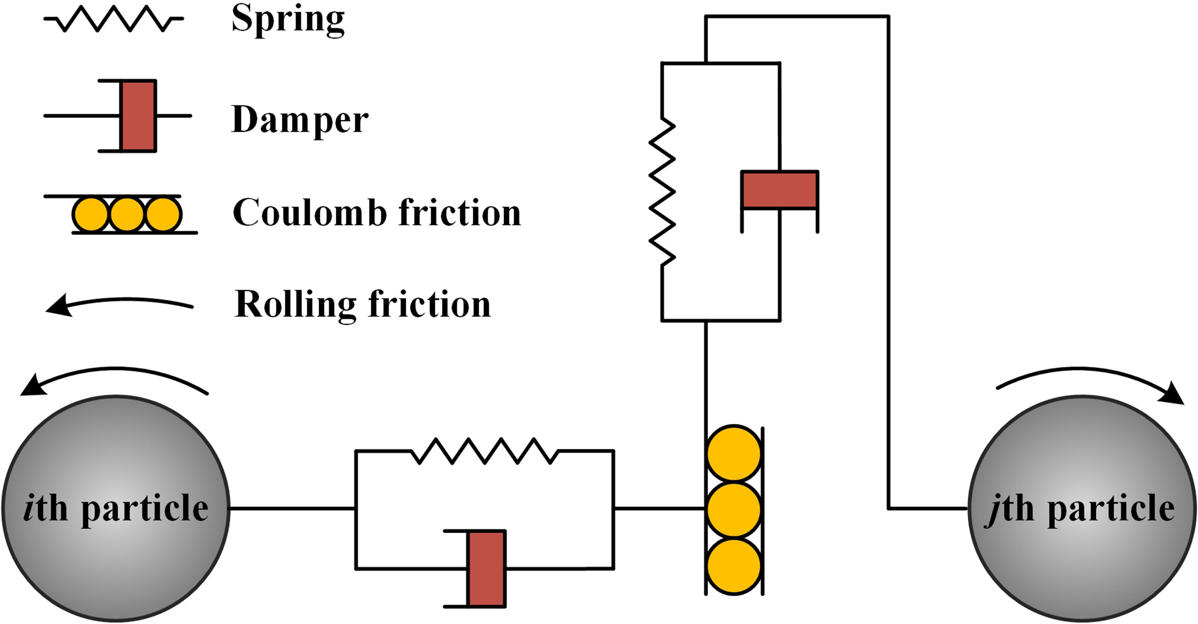
Figure 2 Schematic diagram of Hertz-Mindlin (no-slip) with rolling friction contact model.

$\begin{array}{ll}\begin{array}{c}{F}_{c,ij}=F_{c,ij}^n+F_{c,ij}^t\end{array}& (6)\end{array}$

with

$\begin{array}{ll}\begin{array}{c}{F}_{c,ij}^n=F_{cn,ij}+F_{dn,ij}\end{array}& (7)\end{array}$

and

$\begin{array}{ll}\begin{array}{c}{F}_{c,ij}^t=F_{ct,ij}+F_{dt,ij}\end{array}& (8)\end{array}$

in which $F_{c,ij}^n$ and $F_{c,ij}^t$ represent the normal force and the tangential force between particles. Both two forces consist of the contact component (F_cn,ij and F_ct,ij) and the damping component (F_dn,ij and F_dt,ij). In the normal direction, the contact and damping components can be written as:

$\begin{array}{ll}\begin{array}{c}{\mathit{F}}_{cn,ij}=\frac{4}{3}{E}_{eq}\sqrt{R_{eq}\left|{\mathit{\delta }}_{\mathit{n}}\right|}{\mathit{\delta }}_{\mathit{n}}\end{array}& (9)\end{array}$

$\begin{array}{ll}\begin{array}{c}{\mathit{F}}_{dn,ij}=-2\sqrt{\frac{5}{6}}\beta \sqrt{S_n{m}_{eq}}{v}_n^{\stackrel{\rightharpoonup }{rel}}\end{array}& (10)\end{array}$

with the expression of the critical damping ratio β:

$\begin{array}{ll}\begin{array}{c}\beta =\frac{-\ln e}{\sqrt{{\ln }^{2}e+{\pi }^2}}\end{array}& (11)\end{array}$

here, E_eq is the equivalent Young’s modulus, R_eq is the equivalent radius and δ_n is the normal overlap of the ith particle and the jth particle. In equation (11), e represents the coefficient of restitution, M_eq is the equivalent mass, $v_n^{\stackrel{\rightharpoonup }{rel}}$ is the normal component of the relative velocity between the particles, and S_n is the normal stiffness, which can be defined as:

$\begin{array}{ll}\begin{array}{c}{S}_n=2E_{eq}\sqrt{R_{eq}\left|{\mathit{\delta }}_{\mathit{n}}\right|}\end{array}& (12)\end{array}$

In the tangential direction, the contact and damping components of the forces are described as follows:

$\begin{array}{ll}\begin{array}{c}{\mathit{F}}_{\mathit{c}\mathit{t}\mathit{,}\mathit{i}\mathit{j}}=S_t{\mathit{\delta }}_{\mathit{t}}\end{array}& (13)\end{array}$

$\begin{array}{ll}\begin{array}{c}{\mathit{F}}_{\mathit{d}\mathit{t}\mathit{,}\mathit{i}\mathit{j}}=-2\sqrt{\frac{5}{6}}\beta \sqrt{S_t{m}_{eq}}{v}_t^{\stackrel{\rightharpoonup }{rel}}\end{array}& (14)\end{array}$

where δ_t is the tangential overlap, $v_t^{\stackrel{\rightharpoonup }{rel}}$ is the tangential component of the relative velocity, and S_t is the tangential stiffness defined as:

$\begin{array}{ll}\begin{array}{c}{S}_t=8G_{eq}\sqrt{R_{eq}\left|{\mathit{\delta }}_{\mathit{n}}\right|}\end{array}& (15)\end{array}$

in which G_eq represents the equivalent modulus. Additionally, the calculation of tangential forces between particles should be controlled by Coulomb friction law.

For the consideration of rolling resistance at the particles’ contact region, the contact-independent Constant Directional Torque (CDT) model is applied due to its accurate and efficient computation. The torque model can be expressed as:

$\begin{array}{ll}\begin{array}{c}{\mathit{T}}_{\mathit{i}\mathit{j}}=-{\mu }_r\left|F_{c,ij}^n\right|R^{*}{\mathit{\omega }}_{\mathit{i}j}\end{array}& (16)\end{array}$

where T_ij is the resistive torque, μ_r is the coefficient of rolling friction, R^* is the distance from the contact point to the mass center of a particle, and ω_ij is the unit angular velocity vector at the contact point.

2.3 Two phases coupling

The momentum exchange between the fluid phase and the solid phase is considered by computing the drag force (F_d) as already mentioned in Equation (3). The drag force has been commonly regarded as the most significant force in the two-phase interactions. Here, we adopt the drag force model proposed by Di Felice (1994), which can be defined as:

$\begin{array}{ll}\begin{array}{c}{\mathit{F}}_{\mathit{d}}=\frac{1}{2}{C}_d{\rho }_f\frac{\pi d_p^2}{4}\left|\mathit{u}-\mathit{v}\right|(\mathit{u}\mathit{-}\mathit{v}){ϵ}_f^{-\chi +1}\end{array}& (17)\end{array}$

where d_p is the particle diameter, C_d is the drag force coefficient, v is the particle velocity and the term χ, which is used to correct the influence of solid concentration on the drag force, is given as:

$\begin{array}{ll}\begin{array}{c}\chi =3.7-0.65\exp [-\frac{{(1.5-{\log }_{10}({ϵ}_f{\mathrm{Re}}_p))}^2}{2}]\end{array}& (18)\end{array}$

with

$\begin{array}{ll}\begin{array}{c}R{e}_p=\frac{{\rho }_f{d}_p\left|\mathit{u}\mathit{-}\mathit{v}\right|}{{\mu }_f}\end{array}& (19)\end{array}$

where Re_p is the particle Reynolds number, with μ_f being the fluid dynamic viscosity.

The Di Felice drag model is always used with the drag force coefficient (C_d) given by Dallavalle (1948) in previous studies (Jing et al., 2019; Nian et al., 2021b). In the present study, C_d is replaced by the drag force coefficient proposed by Brown and Lawler (2003) due to it having a wider scope of application and higher accuracy (Zhao et al., 2014). Figure 3 depicts the difference between the drag force coefficients proposed by Dallavalle (1948) and Brown and Lawler (2003), respectively. By referring to Zhao et al. (2014), the drag force coefficient proposed by Brown and Lawler (2003) shows a better agreement with the experimental data, especially in the range of 10²-10⁵ of particle Reynolds numbers. The drag force coefficient C_d is thus given as follows:

FIGURE 3

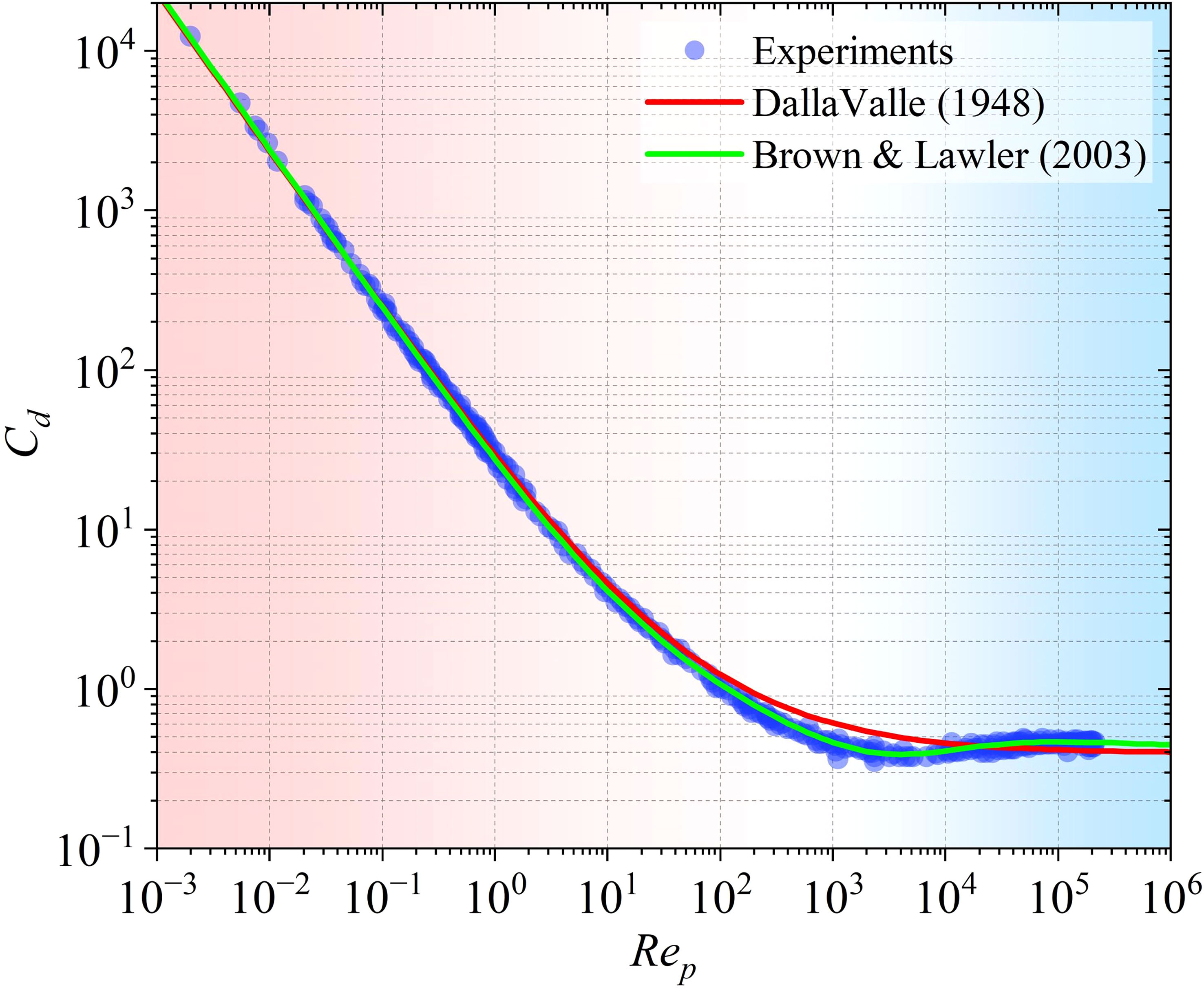
Figure 3 Comparison between different drag force coefficients with the experimental data.

$\begin{array}{ll}\begin{array}{c}{C}_d=\frac{24}{{\text{ϵ}}_{f}R{e}_p}[1+0.150{({\text{ϵ}}_{f}R{e}_p)}^{0.681}]+\frac{0.407}{1+8710/({\text{ϵ}}_{f}R{e}_p)}\end{array}& (20)\end{array}$

According to the abovementioned equations, the drag force model used here is subsequently incorporated into the coupling scheme through user-defined functions (UDFs) in ANSYS FLUENT.

3 Model validation of benchmark cases

3.1 Single particle settling in fluid

To verify the effectiveness of the coupled CFD-DEM model, the benchmark case of a single spherical particle settling in water is first conducted. A spherical particle with a diameter of 1.0 mm and a density of 2650 kg/m³ is released in a rectangular container. The water-filled container is 45 mm in length, 45 mm in width and 120 mm in height, respectively, and the viscosity and density of the water are 0.001 Pa·s and 1000 kg/m³. The particle is initially placed at 40 mm below the top surface of the container and then continues to accelerate until the terminal velocity is reached. For this case, the specific particle motion is described as:

$\begin{array}{ll}\begin{array}{c}\frac{1}{6}\pi d_p^3{\rho }_{p}a=\frac{1}{6}\pi d_p^3({\rho }_p-{\rho }_f)g-\frac{1}{8}\pi d_p^2{\rho }_f{C}_d{v}^2\end{array}& (21)\end{array}$

where ρ_p is the particle density and a is the particle acceleration. Equation (21) can be solved with an iterative solution method to obtain the settling velocity of the particle. It is worth noting that in the unresolved CFD-DEM model, the CFD cell size should be sufficiently large compared to the particle diameter while using the particle counting method for computing the particle concentration field, as suggested by previous studies (Marshall and Sala, 2013; Zhao et al., 2014; Nian et al., 2021b). Here, the computational domain is meshed by hexahedral CFD cells with a size five times the particle diameter, and the time steps of the CFD module and DEM module are 10^-4 s and 10^-5 s, respectively.

The calculated particle settling velocity of the CFD-DEM simulation is compared with that of the analytical one, as shown in Figure 4. Clearly, the simulated settling velocity agrees well with that given by the analytical solution, which validates the proposed CFD-DEM scheme and the drag force model.

FIGURE 4

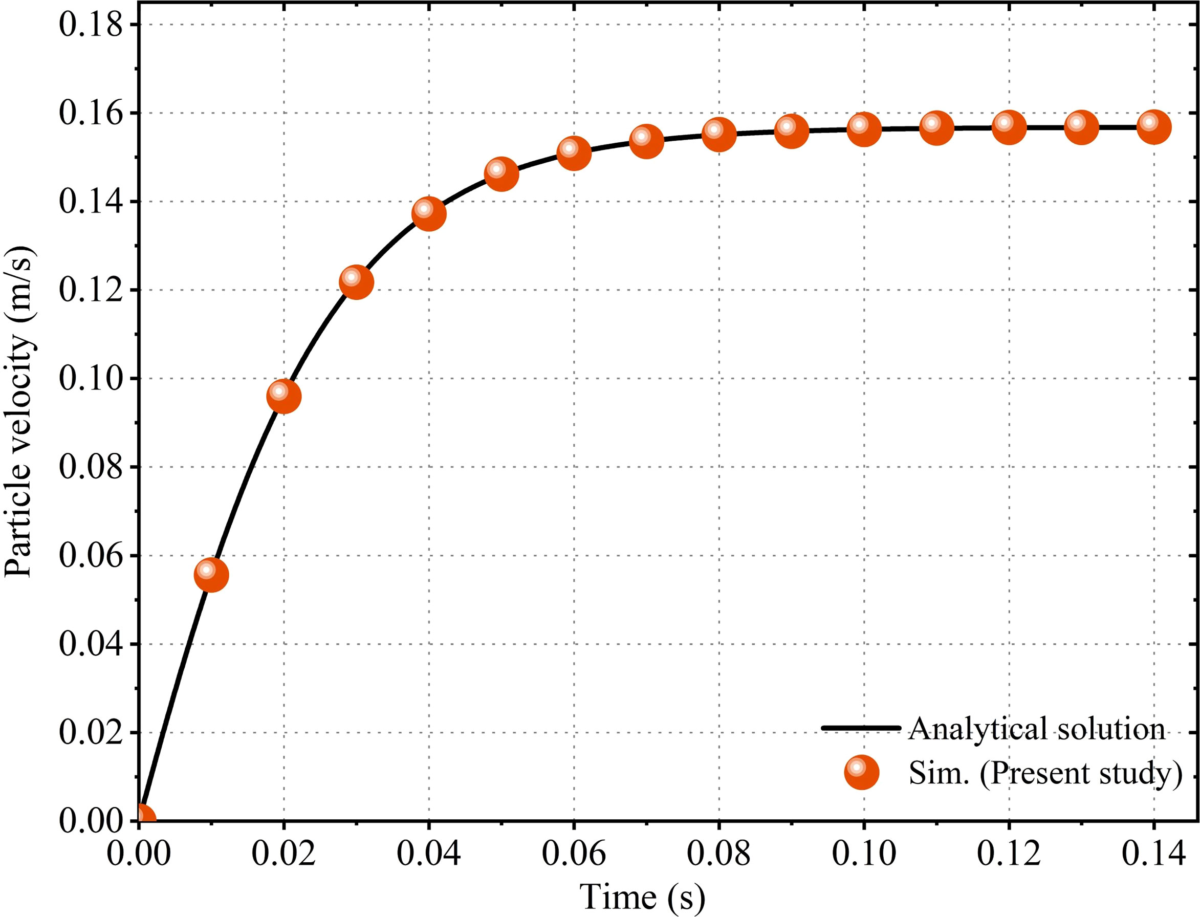
Figure 4 The settling velocity of a particle in water with diameter being 1.0 mm.

3.2 Immersed granular collapse

In the previous section, we gave an accurate prediction of the single-particle velocity by comparing it to the analytical results. However, multi-particle systems are more common and more important in the real world, one of which is submarine landslides (Guo et al., 2023b; Zhang et al., 2023). Submarine landslides can generate enormous turbidity currents with large amounts of sediment (Nisbet and Piper, 1998; Guo et al., 2022). These two marine geological disasters are essentially two types of immersed granular flow characterized by different particle volume concentrations. In the present study, we simulate the collapse and flow process of a granular column immersed in the ambient water through the CFD-DEM model and compare the results with the laboratory experiments conducted by Bougouin and Lacaze (2018). The motivation of this section is to verify the model rationality in simulating a real experiment, both in temporal and spatial scales. The immersed granular column in a laboratory scale is regarded as an idealized model of submarine landslides (or debris flow) and represents a class of high-concentration particulate flow. Because turbidity currents have a high sediment concentration in their near-bed regions, modeling of immersed granular collapse also has significance for simulating the turbidity current propagation.

Bougouin and Lacaze (2018) studied the collapse process of dense-packing granular columns in fluids with different properties, decomposing the collapse processes into four flow regimes (“free-fall”, “inertial”, “viscous inertial” and “viscous” in their study). The experiments selected here are in an inertial regime, which means the granular columns collapse and flow in the water with ρ_f =1000 kg/m³ and μ_f = 0.001 Pa·s. The granular materials used in their experiments is glass beads with ρ_p = 2230 ± 30 kg/m³ and d_p = 3 ± 0.02 mm. The angle of repose and the angle of the avalanche of the glass beads are 22 ± 1° and 28 ± 2°, respectively, which provides a reference for determining the friction coefficient in the DEM module. The granular column of an initial packing density of 0.64 ± 0.02 was placed at a rectangular water tank, and subsequently collapsed in the ambient water once the sluice gate was quickly removed (Figure 5). The initial aspect ratio, a_r = h₀/l₀, is regarded as a key factor that influences the collapse mechanism, runout distance and the final deposit of the granular column. In this study, the aspect ratio of a_r = 1 is chosen to be simulated because the snapshots of this experiment are very clear for comparison. In addition, we noted that the experimental snapshots they used in their study did not strictly match the collapse time of t_f/3, 2 t_f/3, t_f (t_f, the final stopping time of granular collapse) according to the videos they provided in the supplemental material [see the Movie2.avi in the supplemental material of Bougouin and Lacaze (2018)]. For this reason, the selection of the simulation results, which are used to compare with the experiments, refers to the experimental videos. In the numerical cases, the model parameters are set to be the same as the experiments, in which the Poisson’s ratio is 0.25, Young’s modulus is 10⁸ Pa, the coefficient of restitution is 0.65, the coefficient of static friction is 0.53 and the coefficient of rolling friction is 0.01. In this case, the time steps of the CFD module and DEM module are 10^-4 s and 5×10^-6 s, respectively.

FIGURE 5

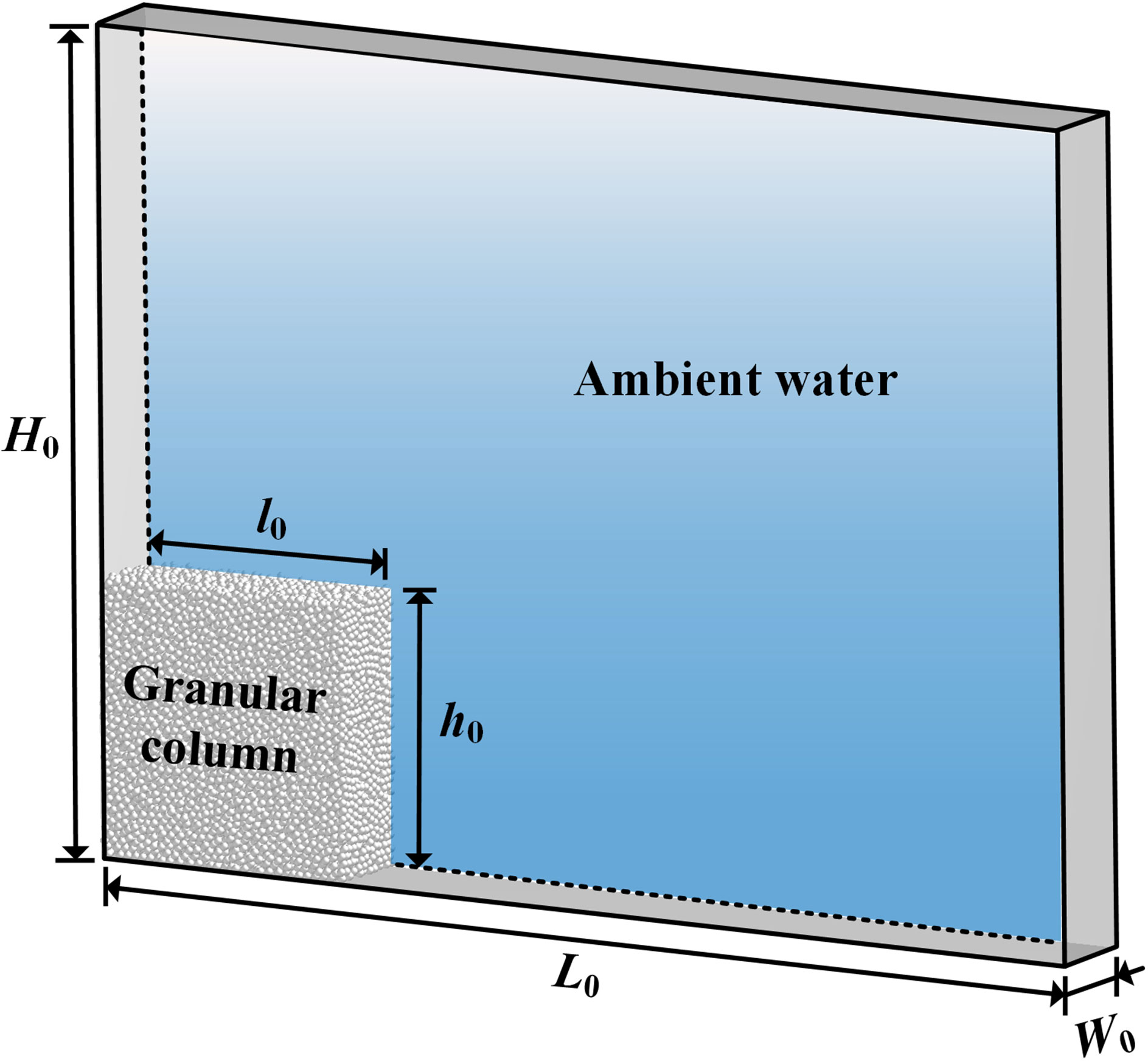
Figure 5 Schematic drawing of the computational set-up of immersed granular collapse. The initial packing length and height of the granular column are l_{0 =} 10 cm and h_{0 =} 10 cm. The dimension of the water tank is 4 l₀ in length (L₀), 3 h₀ in height (H₀) and 3.6 cm in width (W₀).

The time evolution of granular column collapse, both of experiments and numerical simulations, are shown in Figure 6, where the insets indicate the velocity field of the collapsed particles. According to the results, the granular column gradually collapsed into the ambient water with a waveform forming on the granular surface and a relatively thick front. In Figure 6A, the numerical result does not seem to be sufficiently accurate compared to the experiment data, which may result from the influence of sluice gate lifting. In the experimental videos provided by Bougouin and Lacaze (2018), the gate lifting process lasted approximately 0.33 s, which causes a disturbance of ambient water, and subsequently affects the initial motion of the side particles of the granular column. Fortunately, such influence is diminished over time according to the experiment results. At the final moment, the collapsed particles of the physical experiment and the numerical simulation are almost the same morphologically (see Figure 6C). In summary, our simulations accurately reproduce the multi-particle motions within the fluid both in temporal and spatial scales.

FIGURE 6

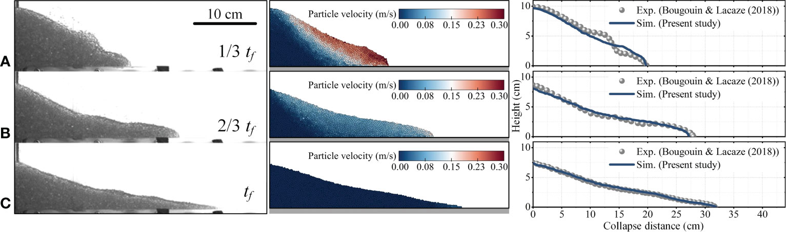
Figure 6 Graphs showing the collapsed morphology at (A) 1/3 t_f, (B) 2/3 t_f, (C) t_f of the physical experiments and the numerical simulations, in which the left panel is the photographs of experiments, the middle panel is the snapshots of numerical simulations, and the right panel is the comparison results.

4 Modeling of turbidity current propagation

4.1 Model setup

Turbidity currents will encounter various kinds of obstacles (e.g., reservoir embankments, submarine cables, pipelines, and seamounts) in their flow paths when propagating in reservoirs or marine environments (Nasr-Azadani et al., 2013). Considerable attention has been devoted to the investigation of the influence of the obstacle on the turbidity currents. Previous studies have used various simplified obstacles (e.g. humpers and circular cylinders) to represent the real seabed topography and marine engineering facilities in their experiments (Kubo, 2004; Ermanyuk and Gavrilov, 2005). Here, we prepare two kinds of simulations to analyze the flow response of turbidity currents to different topographic configurations in a narrow channel, where one is the flat bed case that is regarded as an ideal configuration, and the others are the obstacle-placed cases that are regarded as a simplified obstacle configuration. The obstacles used in those OPB-type cases have rectangular sections with different dimensions as displayed in Figure 7. All the simulations are set up based on a lock-exchange configuration. The lock-exchange (or termed as “lock-release”) experiment is a type of classic experiment for figuring out the fluid mechanics of gravity flows (Gladstone et al., 1998). Commonly, a fixed volume of heavy fluid is separated from light fluid by a sluice gate in a rectangular tank, where the heavy fluid can be the saline water or the fine sediment-water mixture. Once the sluice gate is removed, the heavy fluid propagates as a gravity flow into the ambient light fluid. In our simulations, the ambient fluid is the water, and its basic properties are already given in the benchmark cases. The sediment particle used here has a diameter d_p = 100 μm, which corresponds to the mean particle size of turbidite samples obtained in the South China Sea (Wang et al., 2020). An initial sediment concentration C_i of 1.0% by volume is selected for the particle-water mixture, which is a common value used in turbidity current modeling with CFD methods and within the range of< 9.0% that is given by Bagnold (1962). Additionally, we use periodic boundaries for the two sides of the computational domain in both CFD and DEM. No-slip conditions are imposed along the other boundaries except for the top wall, where the free-slip condition is employed. The parameter settings of the model partially refer to the study of Xie et al. (2022), and the details can be found in Figure 7 and Table 1.

FIGURE 7

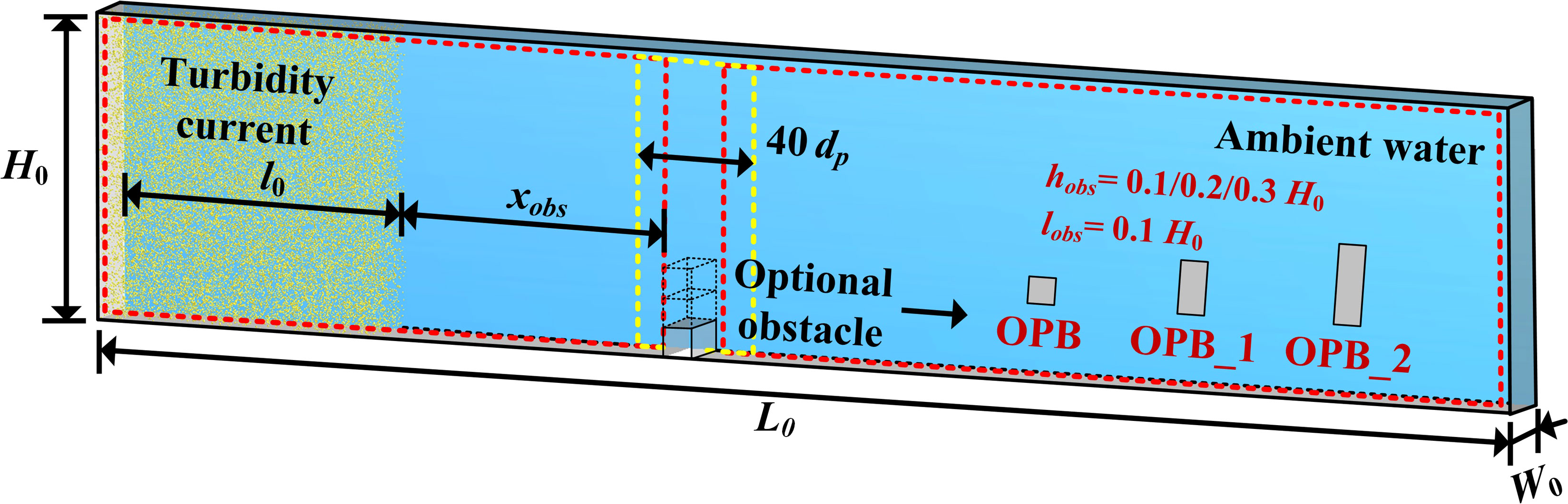
Figure 7 Schematic drawing of the computational set-up of turbidity current propagation, where L_{0 =} 1000 d_p, H₀ = l_{0 =} 200 d_p, and W_{0 =} 40 d_p. In the configuration of the obstacle case, the optional obstacle has a distance x_obs = 200 d_p from the fixed volume of the particle-water mixture, and different rectangular sections.

TABLE 1

Table 1 Model parameters for FB and OPB-type cases.

4.2 Results of FB and OPB-type cases

In the present study, the FB case is treated as a base case for analyzing the dynamics of the sediment particles and the ambient fluid. Figure 8 shows the time evolution of the particle-fluid velocity field from 0.5 s to 4.0 s, where the particles are visualized as balls with a diameter twice the original diameter. At the initial stage of turbidity current propagation, the upper part and lower part of the right side of the particle-water mixture indicate two high fluid-velocity areas in the opposite direction, making an approximately rotating flow field. As indicated by Xie et al. (2022), this phenomenon is caused by the reason that the ambient fluid invades into the particles in the upper part and the particles in the lower part are driven by the flow. Subsequently, the flow head of the turbidity current is gradually formed with a high-velocity core in the head, and the high-velocity core moves backward or even separated into two parts over time due to the drag of the ambient fluid (see 2.5 s and 3.0 s in Figure 8). Consequently, a convex-shaped surface gradually forms, which is similar to the erosion surface of the loosely packed particles after the immersed granular collapse in the study of Jing et al. (2018). These two phenomena are both caused by the vortex-induced fluid shear, indicating that the shape evolution of the particulate flow is highly related to the flow field of the ambient fluid. Specifically in this simulation, the rotating flow drives the particles of the flow tail to move forward but the particles in front of the tail hinder the advance of the rear particles, which leads to the flow tail becoming thinner and the flow body becomes thicker, and several vortices form in the whole channel. Moreover, the numerical results, especially the flow front position x_f, are compared with a classic lock-exchange experiment of turbidity current propagation conducted by Gladstone et al. (1998). By referring to the previous studies (Nasr-Azadani and Meiburg, 2014; Xie et al., 2022), we used the buoyancy velocity u_b and the half-height of the channel H₀/2 as characteristic quantities for scaling the flow variables. The buoyancy velocity can be written as:

FIGURE 8

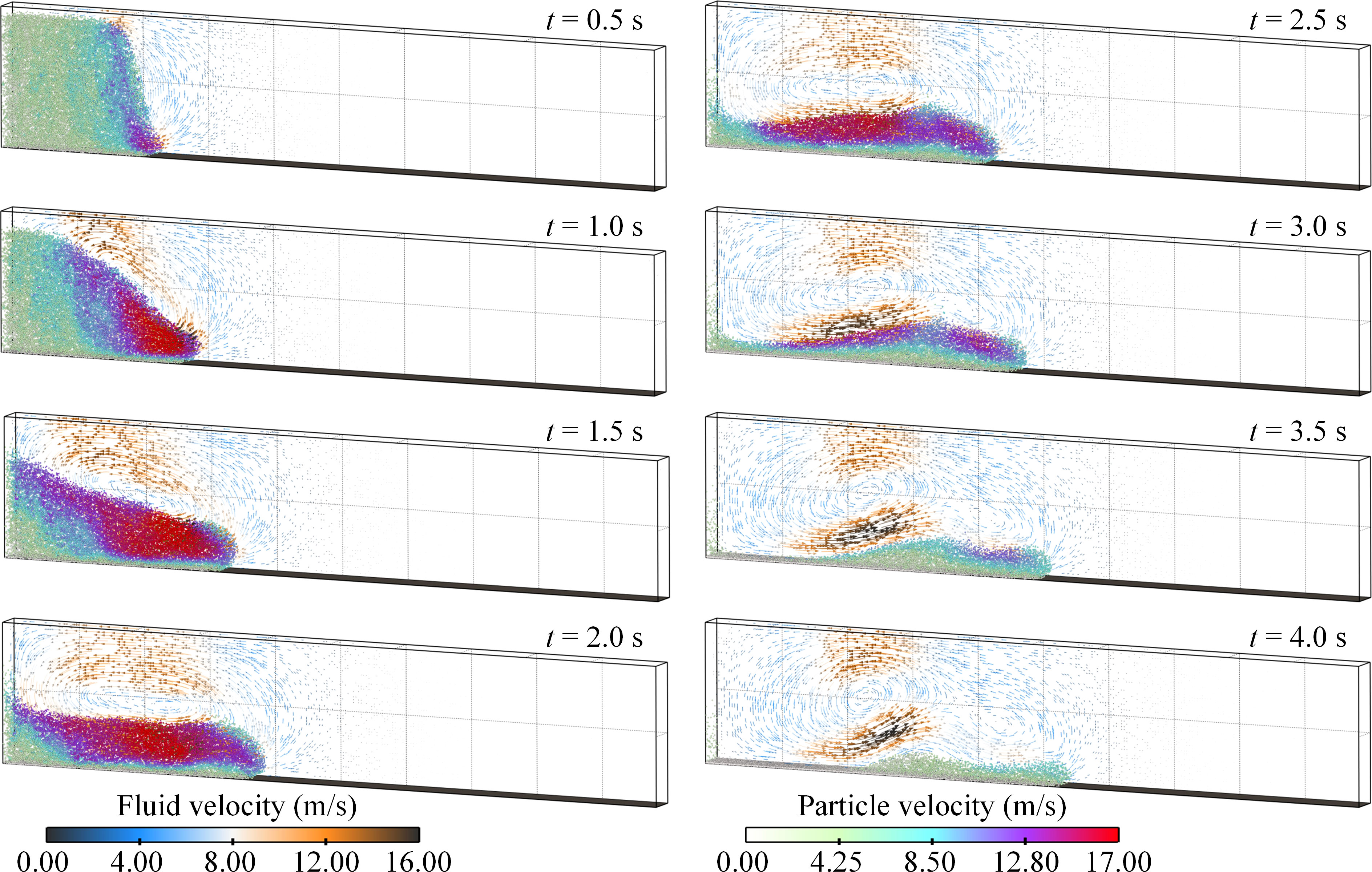
Figure 8 Turbidity current propagation process of FB case. The particle velocity and ambient fluid velocity with vector arrows are shown.

$\begin{array}{ll}\begin{array}{c}{u}_b=\sqrt{g\frac{H_0}{2}\frac{({\rho }_p-{\rho }_f)C_i}{{\rho }_f}}\end{array}& (22)\end{array}$

The numerical results of the dimensionless front position of turbidity current show good consistency with the experimental results as well as the LES-DEM simulation results from Xie et al. (2022), indicating the simulation is accurate (see Figure 9).

FIGURE 9

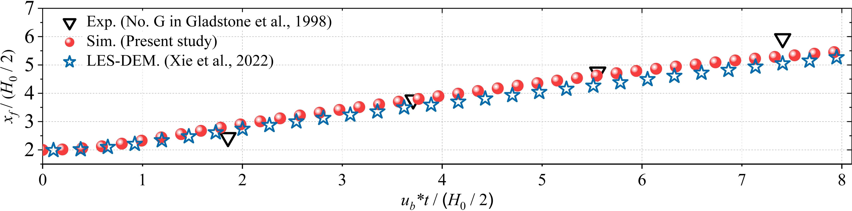
Figure 9 Comparison results of the dimensionless front positions of turbidity currents between the FB case, the experiment in Gladstone et al. (1998) and the numerical simulation in Xie et al. (2022).

In the OPB case, the flow characteristics of turbidity current are almost the same as those in the FB case in the first two seconds except that the fluid velocity of the flow front is larger in the OPB case at 2.0 s (see the velocity vector arrows in Figure 10). Owing to the presence of the simplified obstacle, the fluid and particles have a trend of moving upward, and the flow front gradually becomes thicker. Obviously, the particle velocity of the flow front in the OPB case decreases when it encounters the obstacle. In general, there is no large difference in the flow field developments between both two cases due to the obstacle being relatively small in dimension.

FIGURE 10

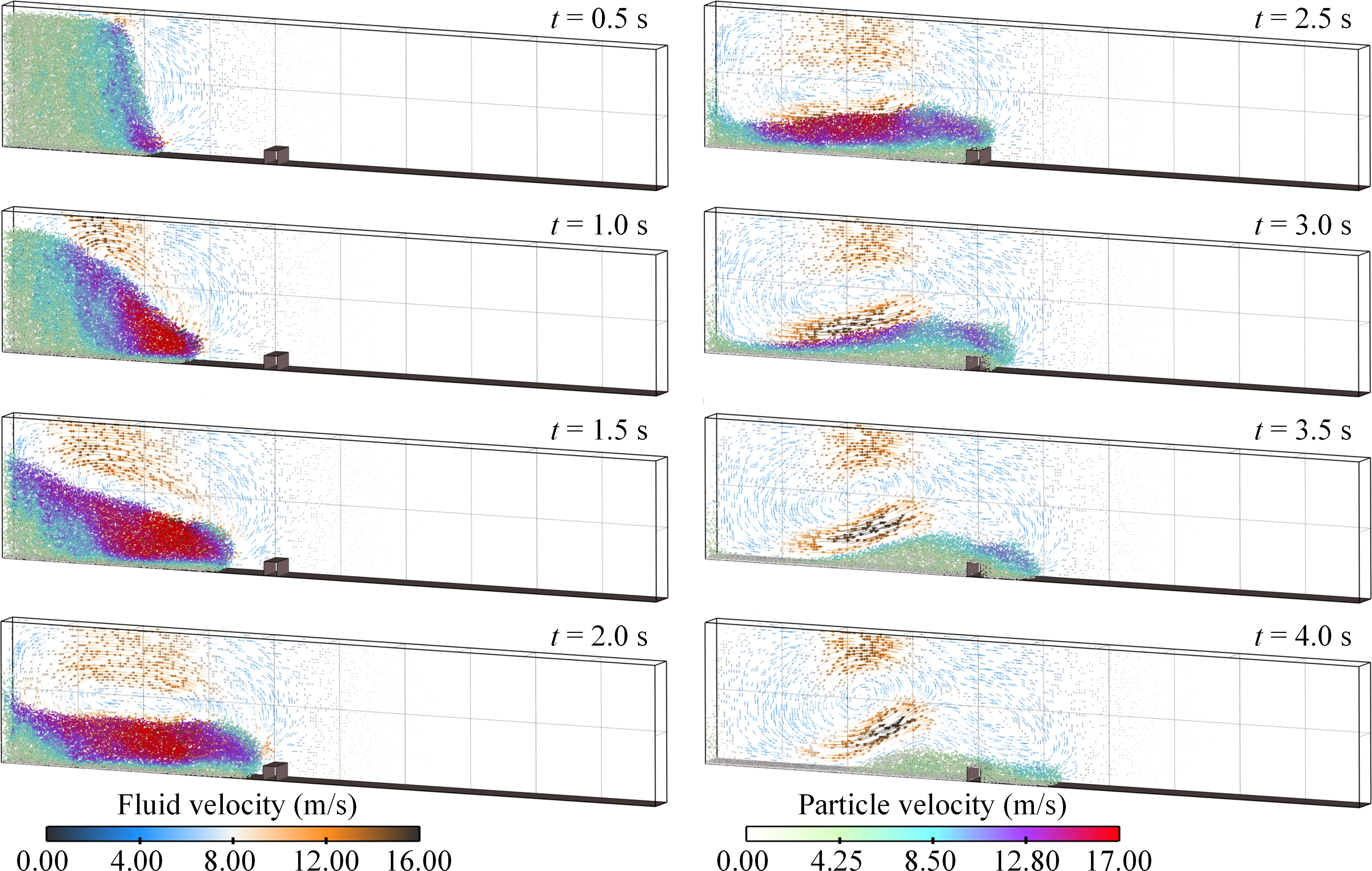
Figure 10 Turbidity current propagation process of the OPB case. The particle velocity and ambient fluid velocity with vector arrows are shown.

However, for OPB_1 and OPB_2 cases, the flow morphologies are diverse from those of FB and OPB cases. Figure 11 depicts the flow morphologies of all the FB and OPB-type cases, and the particle and fluid field are visualized by their velocities in the x-direction. A shear band where the particle velocity are opposite exists in all these four cases. As a result of the increasing obstacle height, the shear band continues to lift, and the particle layer showing negative velocity becomes thicker, indicating that it is more difficult for turbidity current to climbing over the higher obstacle. Forced by the higher obstacle, the particles exhibit diverse flow morphologies, thereby making different flow fields of the ambient fluid (see Figures 11C, D).

FIGURE 11

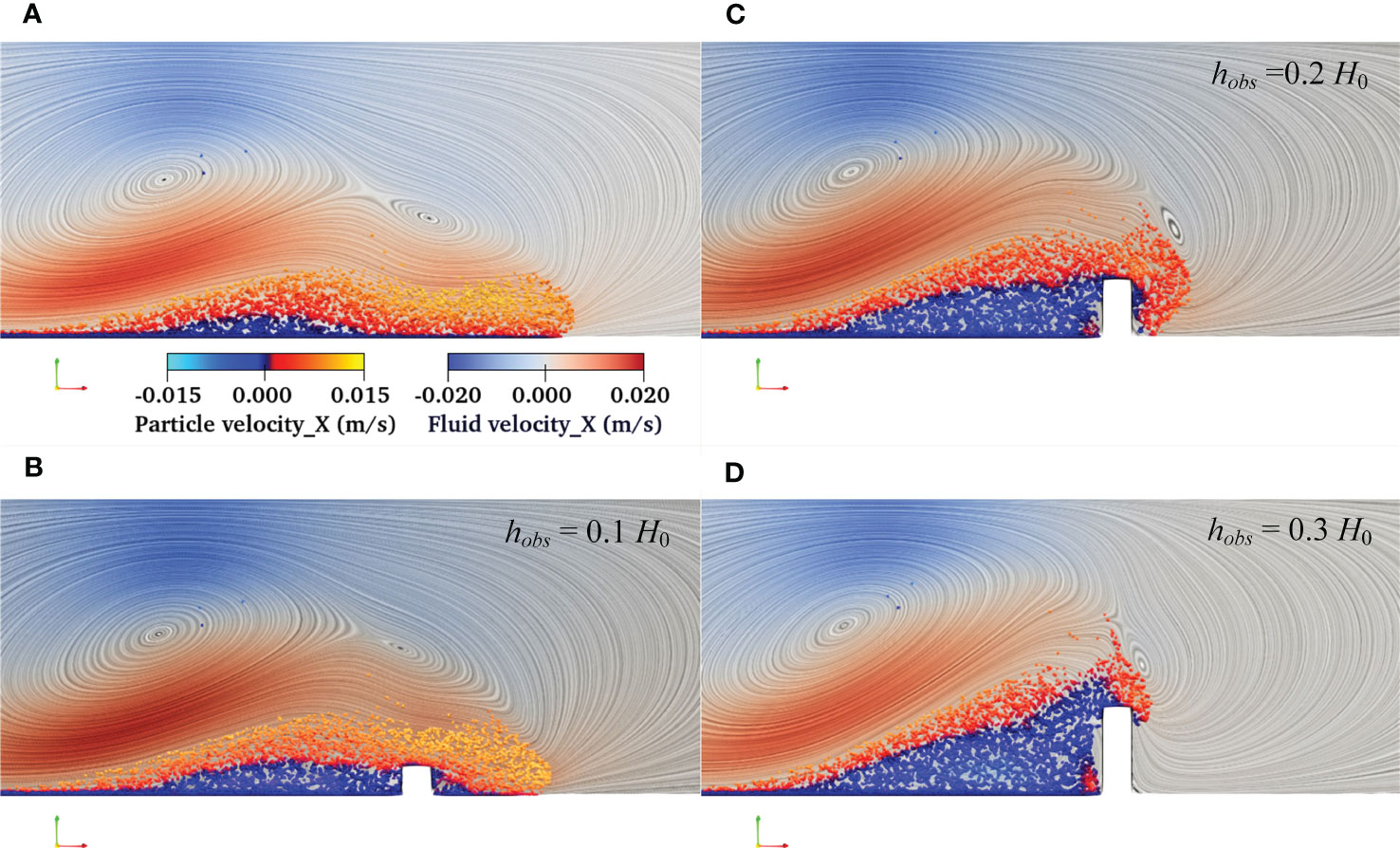
Figure 11 Snapshots of turbidity current propagation over (A) a flat bed, and three obstacle-placed beds with different obstacle heights, specifically, which are (B) h_obs = 0.1 H₀, (C) h_obs = 0.2 H₀, and (D) h_obs = 0.3 H₀. The color maps indicate the particle velocity (balls) and fluid velocity (streamlines) in the x-direction.

4.3 Comparison between FB and OPB-type cases

One of the big advantages of CFD-DEM modeling is that all particle information can be checked out to help us better understand the sediment behaviors in turbidity currents. In this section, we give the comparison results between FB and OPB-type cases, mainly based on the particle information, to show how the simplified obstacle influences the particle motions. To start the comparison, different monitoring regions are set in both two cases to extract the required variables as shown in Figure 7.

Firstly, the particle collision numbers in the global computational domain are counted in Figures 12A, B, in which the collision consists of the inter-particle collision and the particle-bed collision, respectively. In general, the inter-particle collision of each of the three OPB-type cases are slightly weaker than that of the FB case especially at the later stage of the propagation process, indicating that the presence of obstacle does not enhance the particle interactions and the obstacle height has no conspicuous influence on the inter-particle collision. Also in the later stage, the particle-bed collisions are more intense and unstable of the OPB-type cases compared to that of the FB case, which means the contact frequency of particles and underlying bed is higher. In our simulations, the process of particles settling to the bed surface will result in the particle interaction with the bed, which can be characterized by the particle-bed collision. The particle-bed collision results of the OPB-type cases indicate that the presence of the obstacle evidently hinders the particle motions and enhances their sedimentation trends, which is also can be seen in the results of particle kinetic energy (see Figure 12C). The increase of obstacle height indeed affects the particle motions, which is manifested in the increase of particle-bed collision in the later stage and the decrease of particle kinetic energy after encountering the obstacle. Consequently, more particles settle to the bed surface in the left part of (left red-rectangular area in Figure 7) the OPB channel, and the settled particle numbers of the three OPB-type cases (left part) are about 3.5% (OPB), 8.9% (OPB-1) and 13.4% (OPB-2) more than that of the FB case (see Figure 12D).

FIGURE 12

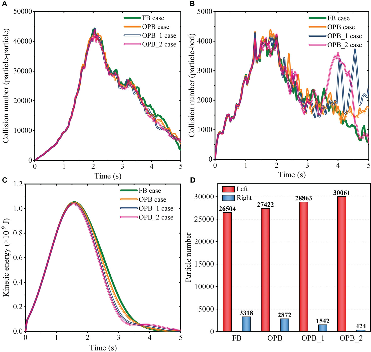
Figure 12 Time evolution of (A) inter-particle collision number, (B) particle-bed collision number, (C) kinetic energy, and (D) particle sedimentation number in the channels of FB and OPB-type cases.

In the adjacent area around the obstacle (yellow rectangular area with 40 d_p in width in Figure 7), the monitoring results exhibit a more obvious regularity in particle dynamics (Figure 13). Clearly, the inter-particle collision numbers of the OPB-type cases are almost always smaller than that of the FB case except at the last stage of turbidity current propagation. At the last stage, the particle-bed collision numbers of the OPB-type cases are also larger than that of the FB case, which is similar to the results in Figure 13A. A reasonable cause is that the particles could settle more efficiently on a flat bed, and it takes longer in the OPB-type cases due to the relatively high elevation of the obstacle. Moreover, the phase-coupling interactions of the OPB-type cases are not as large as expected and even much weaker than that of FB case (see Figure 13C), indicating that the presence of the obstacle can effectively reduce the effect of the ambient water acting on the particles. As the obstacle height increases, the above influences of the obstacle on the particle dynamics are further amplified, although the results of the OPB_1 case show some particularities in its peak values.

FIGURE 13

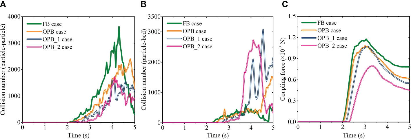
Figure 13 Time evolution of (A) inter-particle collision number, (B) particle-bed collision number, and (C) coupling force in the adjacent area around the obstacle of FB and OPB-type cases.

5 Conclusions

In this study, a fully coupled CFD-DEM model was presented to simulate the turbidity current propagation in a narrow channel. The main conclusions are as follows:

1. In the CFD-DEM model, the drag force coefficient was modified based on the study of Brown and Lawler (2003). To make a step-by-step validation of the model, two benchmark cases, including a single particle sedimentation case and an immersed granular collapse case, were tested by comparing the simulation results to analytic or experimental results. The results of both benchmark cases well verified the effectiveness and accuracy of the CFD-DEM model.

2. The presented model is further applied to the simulation of turbidity current propagation (volume concentration of 1.0%) over two kinds of different bed topographies, consisting of a flat bed and three obstacle-placed beds with different obstacle heights. The FB case reproduced a classic turbidity current that is well consistent with the lock-exchange experiment by comparing the flow front positions, and the flow shape of the turbidity current is highly related to the flow field of ambient fluid.

3. This study also revealed that the presence of the obstacle with different heights result in diverse flow morphologies of particles and fluids. Through the data of the collision number, kinetic energy, coupling force and particle sedimentation number, we concluded that the presence of the obstacle can effectively reduce the propagation velocity and kinetic energy of particles in turbidity currents, and trap about 3.5% (OPB), 8.9% (OPB-1) and 13.4% (OPB-2) more particles in front of the obstacle compared to the FB case. Results also showed that the particle-fluid interactions were weakened around the obstacles.

4. This study exhibits an effective attempt in understanding the interaction between turbidity current and seabed topography, and may provide mesoscopic or microscopic information for large-scale modeling of turbidity currents through combining with other numerical methods (e.g. the μ(I) rheology model). Nonetheless, the current study focused on the interaction process between the turbidity current with spherical particles and the simplified seabed topography with neglecting the influences of the real particle shape and complex topography, which needs to be further concerned in future works.

Data availability statement

The raw data supporting the conclusions of this article will be made available by the authors, without undue reservation.

Author contributions

YL performed the numerical simulation and data analysis and wrote the first draft of the manuscript. XL and XG proposed the work ideas and contributed to the numerical simulation, data analysis, and writing. XX, DL and JS contributed to the data analysis. All authors contributed to the article and approved the submitted version.

Funding

This research was jointly funded by the National Natural Science Foundation of China (42022052 and 42277138), the Shandong Provincial Natural Science Foundation (ZR2020YQ29), and the Fundamental Research Funds for the Central Universities (202161037).

Conflict of interest

The authors declare that the research was conducted in the absence of any commercial or financial relationships that could be construed as a potential conflict of interest.

Publisher’s note

All claims expressed in this article are solely those of the authors and do not necessarily represent those of their affiliated organizations, or those of the publisher, the editors and the reviewers. Any product that may be evaluated in this article, or claim that may be made by its manufacturer, is not guaranteed or endorsed by the publisher.

References

Aas T. E., Howell J. A., Janocko M., Jackson C. A.-L. (2010). Control of aptian palaeobathymetry on turbidite distribution in the buchan graben, outer Moray firth, central north Sea. Mar. Petrol. Geol. 27, 412–434. doi: 10.1016/j.marpetgeo.2009.10.014

CrossRef Full Text | Google Scholar

Abd El-Gawad S. M., Pirmez C., Cantelli A., Minisini D., Sylvester Z., Imran J. (2012). 3-d numerical simulation of turbidity currents in submarine canyons off the Niger delta. Mar. Geol. 326–328, 55–66. doi: 10.1016/j.margeo.2012.06.003

CrossRef Full Text | Google Scholar

Ansys (2017). Fluent theory guide (Canonsburg: Ansys Inc).

Google Scholar

Bagnold R. A. (1962). Auto-suspension of transported sediment, turbidity currents. P. R. Soc A-Math. Phy. 265, 1322. doi: 10.1098/rspa.1962.0012

CrossRef Full Text | Google Scholar

Biegert E., Vowinckel B., Ouillon R., Meiburg E. (2017). High-resolution simulations of turbidity currents. Prog. Earth Planet Sc. 4 (33). doi: 10.1186/s40645-017-0147-4

CrossRef Full Text | Google Scholar

Bougouin A., Lacaze L. (2018). Granular collapse in a fluid: different flow regimes for an initially dense-packing. Phys. Rev. Fluids 3, 64305. doi: 10.1103/PhysRevFluids.3.064305

CrossRef Full Text | Google Scholar

Brown P. P., Lawler D. F. (2003). Sphere drag and settling velocity revisited. J. Environ. Eng. 129, 222–231. doi: 10.1061/(ASCE)0733-9372(2003)129:3(222)

CrossRef Full Text | Google Scholar

Dallavalle J. M. (1948). Micromeritics: the technology of fine particles (London: Pitman Publishing Corporation).

Google Scholar

de Leeuw J., Eggenhuisen J. T., Cartigny M. J. B. (2018). Linking submarine channel-levée facies and architecture to flow structure of turbidity currents, insights from flume tank experiments. Sedimentology 65, 931–951. doi: 10.1111/sed.12411

CrossRef Full Text | Google Scholar

D.E.M. Solutions (2015). Parallel EDEM-CFD coupling for ansys fluent®-user guide (Edinburgh: DEM Solutions Ltd).

Google Scholar

Di Felice R. (1994). The voidage function for fluid-particle interaction systems. Int. J. Multiphas. Flow 20, 153–159. doi: 10.1016/0301-9322(94)90011-6

CrossRef Full Text | Google Scholar

Ermanyuk E. V., Gavrilov N. V. (2005). Interaction of an internal gravity current with a submerged circular cylinder. J. Appl. Mech. Tech. Phys. 46, 216–223. doi: 10.1007/pl00021899

CrossRef Full Text | Google Scholar

Ge Z., Nemec W., Gawthorpe R. L., Hansen E. W. M. (2017). Response of unconfined turbidity current to normal-fault topography. Sedimentology 64, 932–959. doi: 10.1111/sed.12333

CrossRef Full Text | Google Scholar

Ge Z., Nemec W., Gawthorpe R. L., Rotevatn A., Hansen E. W. M. (2018). Response of unconfined turbidity current to relay-ramp topography: insights from process–based numerical modelling. Basin Res. 30, 321–342. doi: 10.1111/bre.12255

CrossRef Full Text | Google Scholar

Gladstone C., Phillips J. C., Sparks R. S. J. (1998). Experiments on bidisperse, constant-volume gravity currents: propagation and sediment deposition. Sedimentology 45, 833–843. doi: 10.1046/j.1365-3091.1998.00189.x

CrossRef Full Text | Google Scholar

Guo X., Liu X., Zhang H., Li M., Luo Q. (2022). Evaluation of instantaneous impact forces on fixed pipelines from submarine slumps. Landslides 19, 2889–2903. doi: 10.1007/s10346-022-01950-3

CrossRef Full Text | Google Scholar

Guo X., Stoesser T., Zheng D., Luo Q., Liu X., Nian T. (2023a). A methodology to predict the run-out distance of submarine landslides. Comput. Geotech. 153, 105073. doi: 10.1016/j.compgeo.2022.105073

CrossRef Full Text | Google Scholar

Guo X., Liu X., Li M., Lu Y. (2023b). Lateral force on buried pipelines caused by seabed slides using a CFD method with a shear interface weakening model. Ocean Eng. 280, 114663. doi: 10.1016/j.oceaneng.2023.114663

CrossRef Full Text | Google Scholar

He Y., Muller F., Hassanpour A., Bayly A. E. (2020). A CPU-GPU cross-platform coupled CFD-DEM approach for complex particle-fluid flows. Chem. Eng. Sci. 223, 115712. doi: 10.1016/j.ces.2020.115712

CrossRef Full Text | Google Scholar

Howlett D. M., Ge Z., Nemec W., Gawthorpe R. L., Rotevatn A., Jackson C. A.-L. (2019). Response of unconfined turbidity current to deep-water fold and thrust belt topography: orthogonal incidence on solitary and segmented folds. Sedimentology 66, 2425–2454. doi: 10.1111/sed.12602

CrossRef Full Text | Google Scholar

Hsu S. K., Kuo J., Yeh Y. C., Tsai C. H. (2008). Turbidity currents, submarine landslides and the 2006 pingtung earthquake off SW Taiwan. Terr. Atmos. Ocean. Sci. 19, 767–772. doi: 10.3319/TAO.2008.19.6.767(PT

CrossRef Full Text | Google Scholar

Hu D., Tang W., Sun L., Li F., Ji X., Duan Z. (2019). Numerical simulation of local scour around two pipelines in tandem using CFD-DEM method. Appl. Ocean. Res. 93, 101968. doi: 10.1016/j.apor.2019.101968

CrossRef Full Text | Google Scholar

Huang H., Imran J., Pirmez C. (2008). Numerical study of turbidity currents with sudden-release and sustained-inflow mechanisms. J. Hydraul. Eng. 134, 1199–1209. doi: 10.1061/(ASCE)0733-9429(2008)134:9(1199

CrossRef Full Text | Google Scholar

Jing L., Yang G. C., Kwok C. Y., Sobral Y. D. (2018). Dynamics and scaling laws of underwater granular collapse with varying aspect ratios. Phys. Rev. E. 98, 42901. doi: 10.1103/PhysRevE.98.042901

CrossRef Full Text | Google Scholar

Jing L., Yang G. C., Kwok C. Y., Sobral Y. D. (2019). Flow regimes and dynamic similarity of immersed granular collapse: a CFD-DEM investigation. Powder Technol. 345, 532–543. doi: 10.1016/j.powtec.2019.01.029

CrossRef Full Text | Google Scholar

Kneller B., Nasr-Azadani M. M., Radhakrishnan S., Meiburg E. (2016). Long-range sediment transport in the world’s oceans by stably stratified turbidity currents. J. Geophys. Res. Oceans 121, 8608–8620. doi: 10.1002/2016JC011978

CrossRef Full Text | Google Scholar

Krause D. C., White W. C., Piper D. J. W., Heezen B. C. (1970). Turbidity currents and cable breaks in the Western new Britain trench. Geol. Soc Am. Bull. 81, 2153–2160. doi: 10.1130/0016-7606(1970)81[2153:TCACBI]2.0.CO;2

CrossRef Full Text | Google Scholar

Kubo Y. S. (2004). Experimental and numerical study of topographic effects on deposition from two-dimensional, particle-driven density currents. Sediment. Geol. 164, 311–326. doi: 10.1016/j.sedgeo.2003.11.002

CrossRef Full Text | Google Scholar

Li P., Kneller B. C., Hansen L., Kane I. A. (2016). The classical turbidite outcrop at San clemente, California revisited: an example of sandy submarine channels with asymmetric facies architecture. Sediment. Geol. 346, 1–16. doi: 10.1016/j.sedgeo.2016.10.001

CrossRef Full Text | Google Scholar

Liu X., Lu Y., Yu H., Ma L., Li X., Li W., et al. (2022). In-situ observation of storm-induced wave-supported fluid mud occurrence in the subaqueous yellow river delta. J. Geophys. Res. Oceans 127, e2021JC018190. doi: 10.1029/2021JC018190

CrossRef Full Text | Google Scholar

Liu X., Wang Y., Zhang H., Guo X. (2023). Susceptibility of typical marine geological disasters: an overview. Geoenviron. Disasters 10, 10. doi: 10.1186/s40677-023-00237-6

CrossRef Full Text | Google Scholar

Lube G., Breard E. C. P., Esposti-Ongaro T., Dufek J., Brand B. (2020). Multiphase flow behaviour and hazard prediction of pyroclastic density currents. Nat. Rev. Earth Env. 1, 348–365. doi: 10.1038/s43017-020-0064-8

CrossRef Full Text | Google Scholar

Lucchese L. V., Monteiro L. R., Schettini E. B. C., Silvestrini J. H. (2019). Direct numerical simulations of turbidity currents with evolutive deposit method, considering topography updates during the simulation. Comput. Geotech. 133, 104306. doi: 10.1016/j.compgeo.2021.104438

CrossRef Full Text | Google Scholar

Marshall J. S., Sala K. (2013). Comparison of methods for computing the concentration field of a particulate flow. Int. J. Multiph. Flow 56, 4–13. doi: 10.1016/j.ijmultiphaseflow.2013.05.009

CrossRef Full Text | Google Scholar

Meiburg E., Kneller B. (2010). Turbidity currents and their deposits. Annu. Rev. Fluid Mech. 42, 135–156. doi: 10.1146/annurev-fluid-121108-145618

CrossRef Full Text | Google Scholar

Nasr-Azadani M. M., Hall B., Meiburg E. (2013). Polydisperse turbidity currents propagating over complex topography: comparison of experimental and depth-resolved simulation results. Comput. Geotech. 53, 141–153. doi: 10.1016/j.cageo.2011.08.030

CrossRef Full Text | Google Scholar

Nasr-Azadani M. M., Meiburg E. (2014). Turbidity currents interacting with three-dimensional seafloor topography. J. Fluid Mech. 745, 409–443. doi: 10.1017/jfm.2014.47

CrossRef Full Text | Google Scholar

Nian T., Li D., Liang Q., Wu H., Guo X. (2021a). Multi–phase flow simulation of landslide dam formation process based on extended coupled DEM-CFD method. Comput. Geotech. 140, 104438. doi: 10.1016/j.compgeo.2021.104438

CrossRef Full Text | Google Scholar

Nian T., Wu H., Takara K., Li D., Zhang Y. (2021b). Numerical investigation on the evolution of landslide-induced river blocking using coupled DEM-CFD. Comput. Geotech. 134, 104101. doi: 10.1016/j.compgeo.2021.104101

CrossRef Full Text | Google Scholar

Nisbet E. G., Piper D. J. W. (1998). Giant submarine landslides. Nat 392, 329–330. doi: 10.1038/32765

CrossRef Full Text | Google Scholar

Plink-Björklund P., Steel R. J. (2004). Initiation of turbidity currents: outcrop evidence for Eocene hyperpycnal flow turbidites. Sediment. Geol. 165, 29–52. doi: 10.1016/j.sedgeo.2003.10.013

CrossRef Full Text | Google Scholar

Pohl F., Eggenhuisen J. T., Tilston M., Cartigny M. J. B. (2019). New flow relaxation mechanism explains scour fields at the end of submarine channels. Nat. Commun. 10, 4425. doi: 10.31223/osf.io/buknq

PubMed Abstract | CrossRef Full Text | Google Scholar

Sun R., Xiao H. (2016). SediFoam: a general-purpose, open-source CFD-DEM solver for particle-laden flow with emphasis on sediment transport. Comput. Geosci. 89, 207–219. doi: 10.1016/j.cageo.2016.01.011

CrossRef Full Text | Google Scholar

Talling P. J. (2013). Hybrid submarine flows comprising turbidity current and cohesive debris flow: deposits, theoretical and experimental analyses, and generalized models. Geosph 9, 460–488. doi: 10.1130/GES00793.1

CrossRef Full Text | Google Scholar

Vellinga A. J., Cartigny M. J. B., Eggenhuisen J. T., Hansen E. W. M. (2018). Morphodynamics and depositional signature of low-aggradation cyclic steps: new insights from a depth-resolved numerical model. Sedimentology 65, 540–560. doi: 10.1111/sed.12391

CrossRef Full Text | Google Scholar

Vowinckel B. (2021). Incorporating grain-scale processes in macroscopic sediment transport models. Acta Mech. 232, 2023–2050. doi: 10.1007/s00707-021-02951-4

CrossRef Full Text | Google Scholar

Wang X., Wang Y., Tan M., Cai F. (2020). Deep-water deposition in response to sea-level fluctuations in the past 30 kyr on the northern margin of the south China Sea. Deep-Sea Res. PT I. 163, 103317. doi: 10.1016/j.dsr.2020.103317

CrossRef Full Text | Google Scholar

Xie J., Hu P., Pähtz T., He Z., Cheng N. (2022). Fluid-particle interaction regimes during the evolution of turbidity currents from a coupled LES/DEM model. Adv. Water Resour. 163, 104171. doi: 10.1016/j.advwatres.2022.104171

CrossRef Full Text | Google Scholar

Xu W. J., Dong X. Y., Ding W. T. (2019). Analysis of fluid-particle interaction in granular materials using coupled SPH-DEM method. Powder Technol. 353, 459–472. doi: 10.1016/j.powtec.2019.05.052

CrossRef Full Text | Google Scholar

Yang G. C., Jing L., Kwok C. Y., Sobral Y. D. (2019). A comprehensive parametric study of LBM-DEM for immersed granular flows. Comput. Geotech. 114, 103110. doi: 10.1016/j.compgeo.2019.103100

CrossRef Full Text | Google Scholar

Zhang H., Lu Y., Liu X., Li X., Wang Z., Ji C., et al. (2023). Morphology and origin of liquefaction-related sediment failures on the yellow river subaqueous delta. Mar. Petrol. Geol. 153, 106262. doi: 10.1016/j.marpetgeo.2023.106262

CrossRef Full Text | Google Scholar

Zhao T., Houlsby G. T., Utili S. (2014). Investigation of granular batch sedimentation via DEM-CFD coupling. Granul. Matter 16, 921–932. doi: 10.1007/s10035-014-0534-0

CrossRef Full Text | Google Scholar

Zhu R., He Z., Zhao K., Vowinckel B., Meiburg E. (2022). Grain-resolving simulations of submerged cohesive granular collapse. J. Fluid Mech. 942, A49. doi: 10.1017/jfm.2022.404

CrossRef Full Text | Google Scholar